
A Review of Estimation Methods for Aboveground Biomass in Grasslands Using UAV

 , , and
Abstract
:1. Introduction
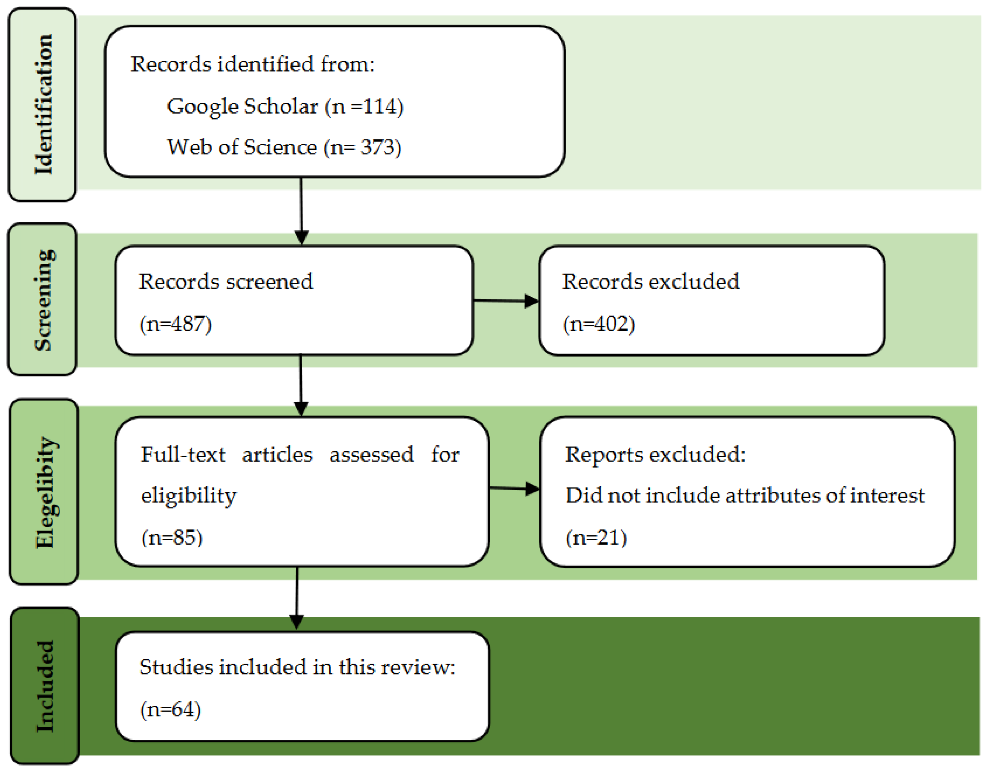
2. Materials and Methods
3. Results and Discussion
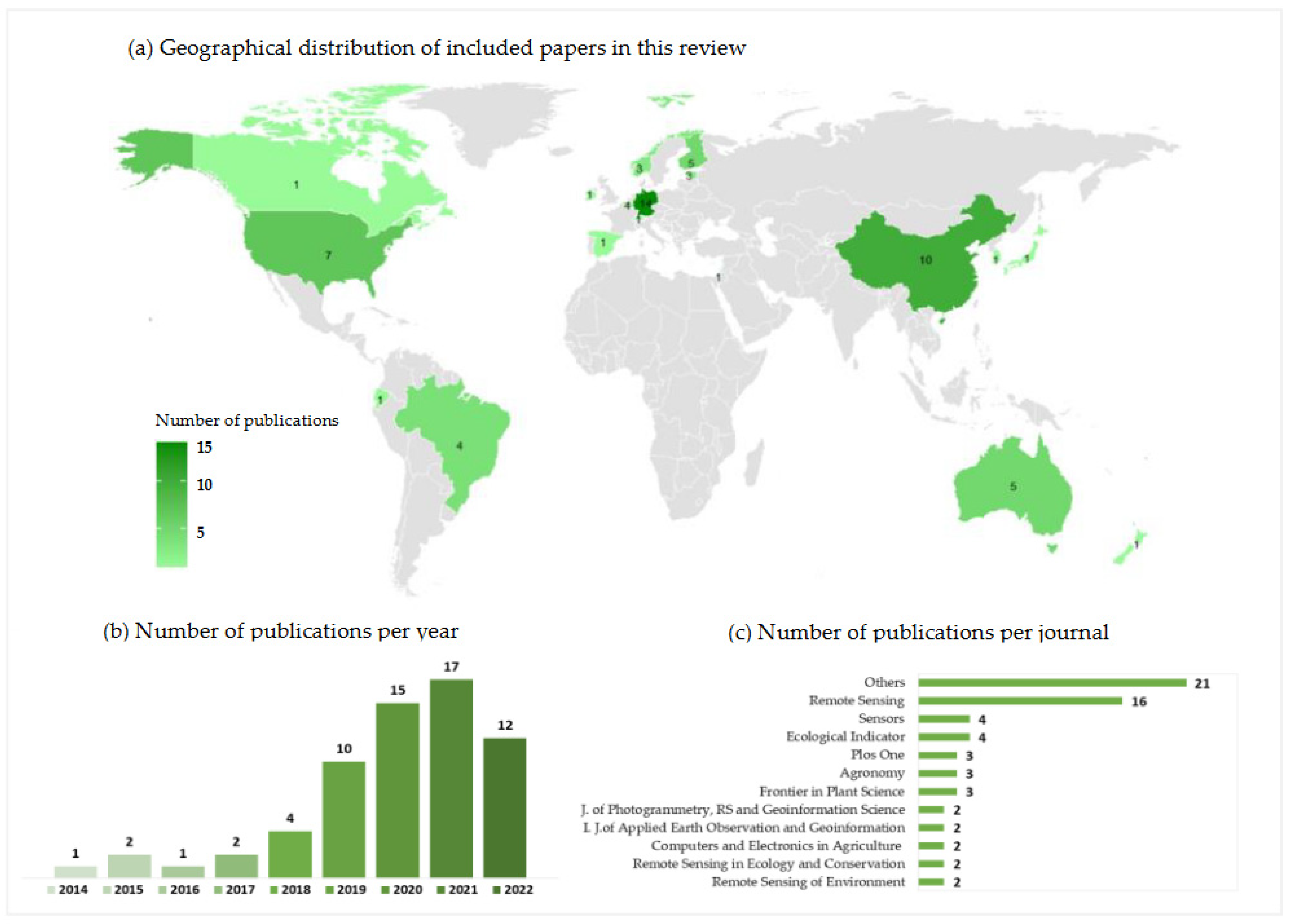
3.1. General Characteristics of Studies
3.2. Characteristics of the Study Sites
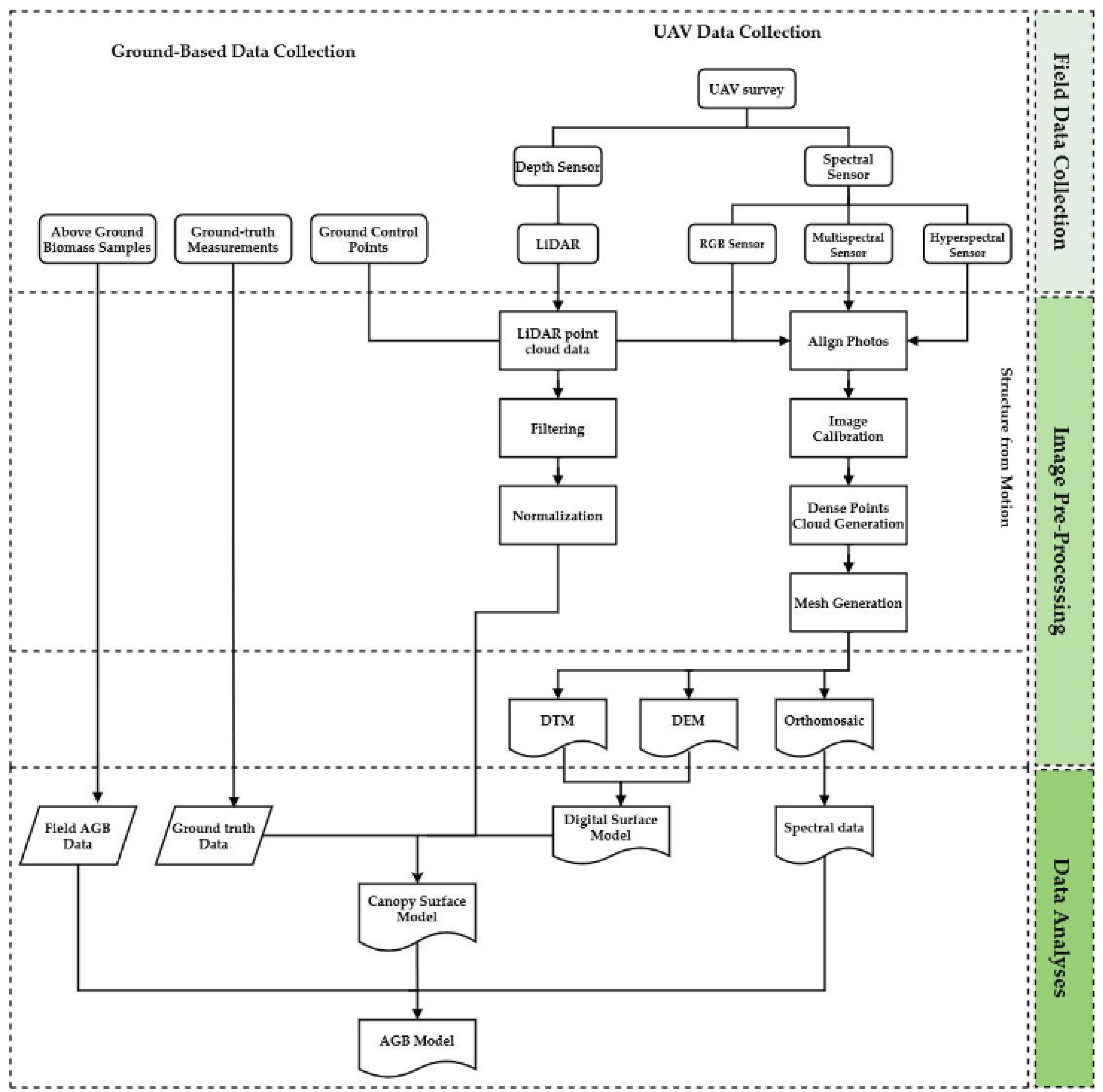
3.3. UAV Data Collection, UAV Data Processing, and Analysis Methods
3.3.1. Field Data Collection
Ground-Based Data Collection
UAV Platforms
Flight Parameters
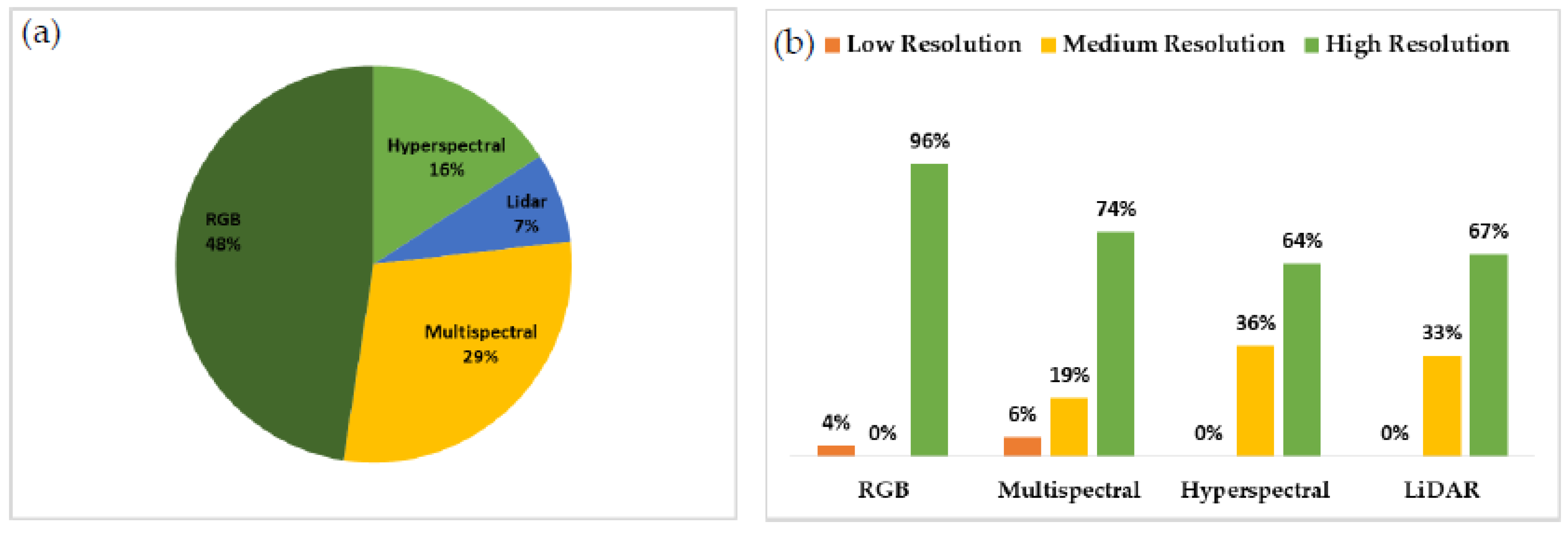
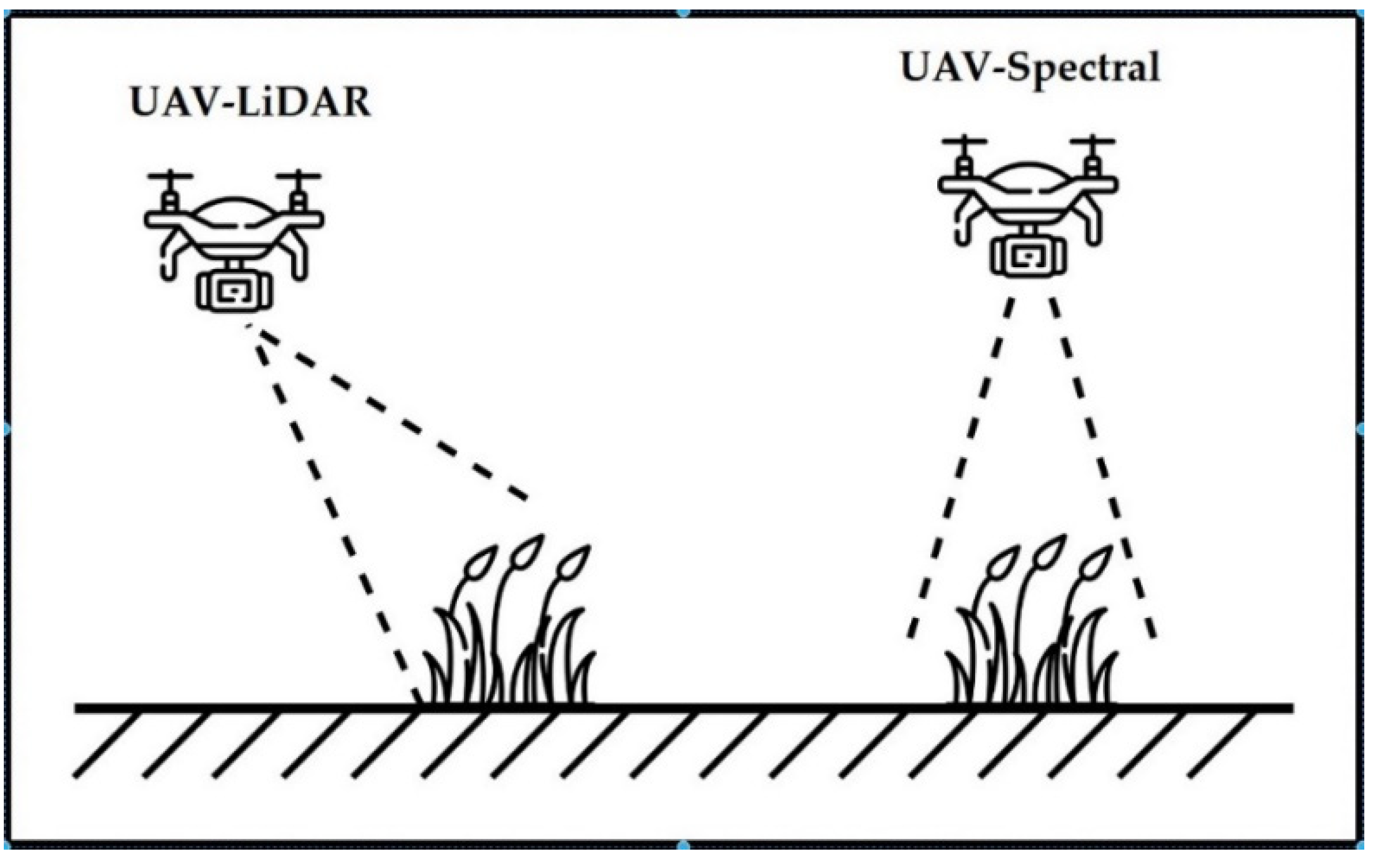
Sensor Technology
3.3.2. Image Pre-Processing
3.3.3. Data Analyses
Inputs
4. Challenges and Future Prospects
5. Conclusions
- The frequency of publications on grassland AGB estimation with UAV has increased over time and continues to rise, indicating the scientific community’s interest.
- The frequency of studies is poorly distributed around the world, with South American and African grasslands appearing to be underrepresented. As a result, additional research should be conducted on some important grassland areas.
- The type of grassland, the heterogeneity, and the growth stage can strongly influence the AGB estimation model.
- Collecting ground-based data is a crucial step in estimating AGB in grasslands. The biomass sampling method seems to have a small influence on the accuracy of the AGB model estimation, whereas the number of samples is one of the main factors to improve the estimation accuracy.
- The measurement of canopy height is an important variable, especially for models that use structural data as input. However, the methods for collecting canopy height at the field level present limitations. RPM measurements demonstrated lower accuracy in sparse swards or tall, non-uniform canopies, and a measuring tape is based on an “average height”, but determined visually and rather subjective. The biases of each method must be taken into account to reduce inconsistencies in the results.
- Quadcopters were the most widely used platform, accounting for almost 60% of all platforms. Nevertheless, the type of platform has a low impact in AGB grassland estimation, and the selection of the platform depends more on the research objective.
- The modal value for UAV flight altitude among the studies was 50 m. Adopting lower altitude flights seems to enhance AGB estimations as this increase the spatial resolution. For farm-scale applications, however, collecting UAV data at higher altitude offers more advantages. We suggest flying at the highest altitude where the desirable GSD is possible.
- Large image forward and side overlaps of approximately 80%, combined with self-calibration during photogrammetric processing, can provide better data quality.
- In terms of sensor type, RGB was the most commonly employed (48%). Despite MS and HS sensor has the advantage to provide more spectral bands RGB data seems capable to produce models with comparable accuracy. In terms of cost–benefit and data processing simplicity, RGB sensors appear to be the most suitable for estimating AGB in grassland at the moment. The emergence of reliable and cost-effective LiDAR and hyperspectral sensors will have a significant impact on future research.
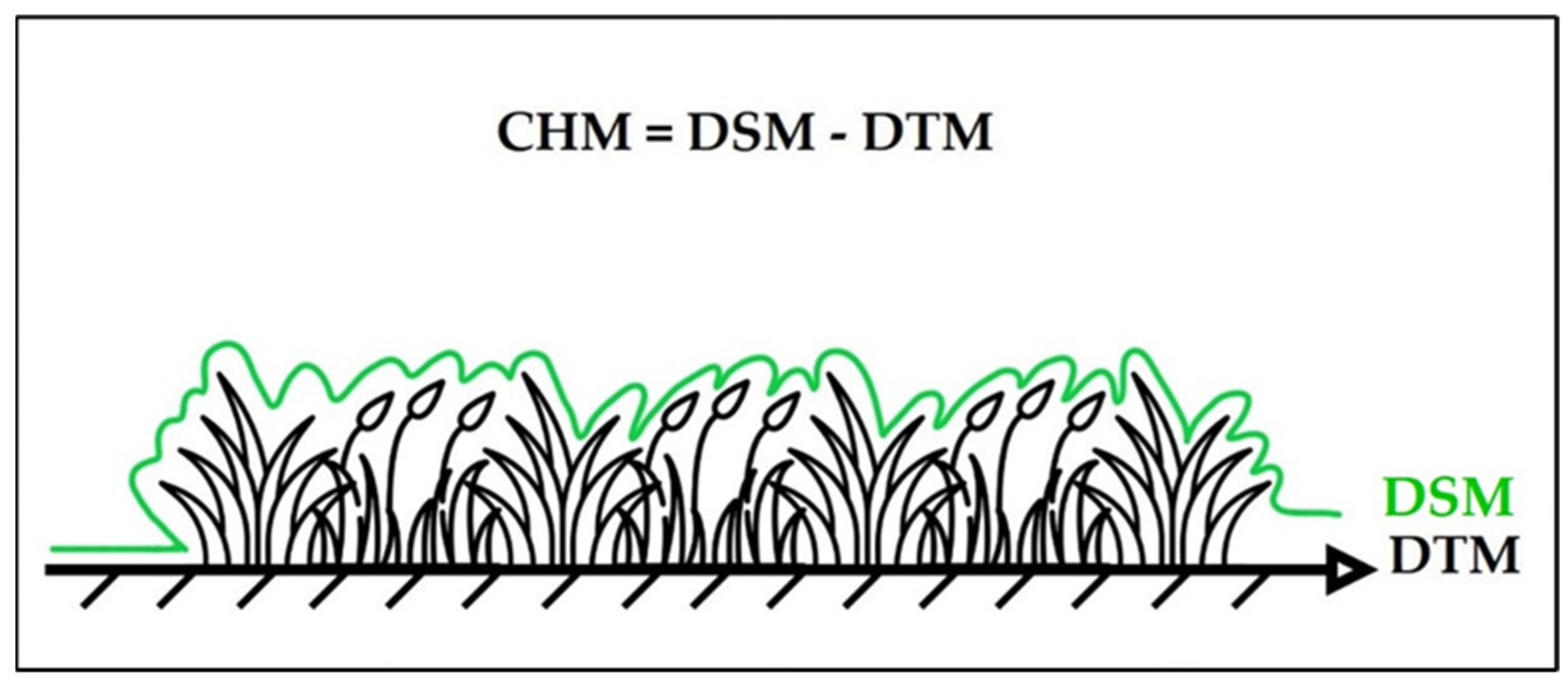
- For the reliable estimation of vegetation structure in grasslands from UAV imagery, a high-quality DTM with a precise and accurate representation of the terrain is necessary. However, UAV-derived DTMs may underestimate or overestimate field terrain differences depending on the canopy’s density and the spatial resolution of the image.
- The accuracy of georeferencing models increases when a larger number of ground control points are equally distributed throughout the study area.
- Linear regression was the most commonly used regression model (n = 25). Random forest was the most popular machine learning method (n = 16). The findings suggest that the accuracy of the analysis methods is more dependent on the quantity and quality of data from field samples rather than the method itself.
- The most common inputs for AGB prediction in grasslands using UAV are spectral and structural data. Canopy height metrics were the most used structural data. At least 68% of the articles used vegetation indices for biomass estimation, with NDVI being the most commonly used. The results indicate that models that employed both data types (structural and spectral) outperformed models that only used one.
Author Contributions
Funding
Data Availability Statement
Acknowledgments
Conflicts of Interest
Appendix A

| No. | Title | Ref | Year | Journal | Main Objective |
|---|---|---|---|---|---|
| 1 | Modeling above-ground biomass in tallgrass prairie using ultra-high spatial resolution sUAS imagery | [41] | 2014 | Photogrammetric Engineering & Remote Sensing | To examine relationship between herbaceous AGB for the tallgrass prairie and its biophysical parameters derived from ultra-high-spatial-resolution imagery. |
| 2 | Estimating plant traits of grasslands from UAV-acquired hyperspectral images: a comparison of statistical approaches. | [57] | 2015 | International Journal of Geo-Information | To investigate the utility of hyperspectral images acquired from UAV for predicting vegetation traits in grasslands considering the plant phenology and fertilization on spectral data. |
| 3 | Mapping Herbage Biomass on a Hill Pasture using a Digital Camera with an Unmanned Aerial Vehicle System | [84] | 2015 | Journal of The Korean Society of Grassland and Forage Science | To develop a simple and cost-effective low-altitude aerial platform system with a commercial digital camera on an UAV system to collect images and estimate the herbage biomass using statistical analyses. |
| 4 | Ultra-fine grain landscape-scale quantification of dryland vegetation structure with drone-acquired structure-from-motion photogrammetry | [59] | 2016 | Remote Sensing of Environment | To develop a new technique to quantify biomass and associated carbon stocks in heterogeneous and dynamic short sward semi-arid rangelands. |
| 5 | Hyperspectral aerial imaging for grassland yield estimation | [104] | 2017 | Advances in Animal Biosciences | To investigate the potential of UAV imaging spectroscopy for in-season grassland yield estimation. |
| 6 | Modeling Aboveground Biomass in Hulunber Grassland Ecosystem by Using Unmanned Aerial Vehicle Discrete Lidar | [72] | 2017 | Sensors | To investigate if the canopy height, fraction cover, and aboveground biomass can be derived using models established from UAV-based discrete LIDAR data with desirable accuracy at quadrat and subplot scales. |
| 7 | Low-cost visible and near-infrared camera on an unmanned aerial vehicle for assessing the herbage biomass and leaf area index in an Italian ryegrass field | [85] | 2018 | Grassland Sciences | To demonstrate the use of a UAV system equipped with a low-cost visible and near-infrared (V-NIR) camera to assess the spatial variability in herbage biomass and LAI in an Italian ryegrass field. |
| 8 | Estimating biomass and nitrogen amount of barley and grass using UAV and aircraft based spectral and photogrammetric | [83] | 2018 | Remote Sensing | To develop and assess a methodology for crop biomass and nitrogen estimation, integrating spectral and 3D features that can be extracted using airborne miniaturized multispectral, hyperspectral, and color (RGB) cameras. |
| 9 | A novel machine learning method for estimating biomass of grass swards using a photogrammetric canopy height model, images and vegetation indices captured by a drone. | [26] | 2018 | Agriculture | To develop and assess a novel machine learning technique for the estimation of canopy height and biomass of grass swards utilizing multispectral photogrammetric camera data. |
| 10 | Estimation of Grassland Canopy Height and Aboveground Biomass at the Quadrat Scale Using Unmanned Aerial Vehicle | [8] | 2018 | Remote Sensing | To develop a novel method for estimating the quadrat-scale aboveground biomass of low-statute vegetation. |
| 11 | Evaluation of grass quality under different soil management scenarios using remote sensing techniques. | [98] | 2019 | Remote Sensing | To evaluate the efficiency of hyperspectral and multispectral (UAV and satellite) remote sensing techniques for predicting and mapping grass biomass and crude protein under conventional grassland management in a temperate maritime climate. |
| 12 | Estimating pasture biomass and canopy height in Brazilian savanna using UAV photogrammetry. | [70] | 2019 | Remote Sensing | To estimate the canopy height using UAV photogrammetry and to propose an equation for the estimation of biomass of Brazilian savanna (Cerrado) pastures based on UAV canopy height. |
| 13 | Canopy height measurements and non-destructive biomass estimation of Lolium perenne swards using UAV imagery. | [54] | 2019 | Grass and Forage Science | To develop a methodology for monitoring the spatial and temporal dynamics of biomass accumulation of perennial ryegrass plots throughout the growing season in an affordable, easy-to-use, reliable, and non-destructive way using an RGB camera mounted on a UAV. |
| 14 | Biomass Prediction of Heterogeneous Temperate Grasslands Using an SfM Approach Based on UAV Imaging | [71] | 2019 | Agronomy | To develop of prediction models for dry matter yield in temperate grassland based on canopy height data generated by UAV RGB imaging over a whole growing season including four cuts. |
| 15 | Estimation of spatial and temporal variability of pasture growth and digestibility in grazing rotations coupling unmanned aerial vehicle (UAV) with crop simulation models | [68] | 2019 | PLOS One | To monitor, assess and manage changes in pasture growth, morphology, and digestibility by integrating information from an UAV and two process-based models. |
| 16 | Estimating biomass in temperate grassland with high resolution canopy surface models from UAV-based RGB images and vegetation indices | [18] | 2019 | Journal of Applied Remote Sensing | To evaluate the potential of low-cost UAV-based canopy surface models to monitor sward height as an indicator of grassland biomass and compare with established methods for biomass monitoring. |
| 17 | Mapping and monitoring of biomass and grazing in pasture with an unmanned aerial system | [67] | 2019 | Remote Sensing | To evaluate the potential of UAV as a tool for the characterization of pasture 3D structure (sward height) and aboveground biomass at a very fine spatial scale. |
| 18 | Comparing UAV-Based Technologies and RGB-D Reconstruction Methods for Plant Height and Biomass Monitoring on Grass Ley | [37] | 2019 | Sensors | To evaluate aerial and on-ground methods to characterize grass ley fields, composed of different species mixtures and estimate plant height, biomass and volume, using digital grass models, and avoiding the unnecessary destruction of the swards. |
| 19 | Evaluating soil-borne causes of biomass variability in grassland by remote and proximal sensing | [73] | 2019 | Sensors | To investigate the relationship between soil characteristics and biomass production to identify high- and low-yielding regions within the field and their possible soil-borne causes. |
| 20 | Evaluation of 3D point cloud-based models for the prediction of grassland biomass | [44] | 2019 | International Journal of Applied Earth Observation and Geoinformation | To evaluate 3D point clouds derived from a terrestrial laser scanner (TLS) and an UAV-borne SfM approach for grassland biomass estimation over three grasslands with different composition and management practice in northern Hesse, Germany. |
| 21 | Estimating Plant Pasture Biomass and Quality from UAV Imaging across Queensland’s Rangelands | [25] | 2020 | AgriEngineering | To demonstrate the use of UAV hyperspectral remote sensing to detect both crude protein and acid detergent fiber in a range of native pastures across the rangelands of Queensland, Australia. |
| 22 | Deep learning applied to phenotyping of biomass in forages with UAV-based RGB imagery | [96] | 2020 | Sensors | To propose a deep learning approach to estimate biomass in forage breeding programs and pasture fields using only UAV-RGB imagery and AlexNet and ResNet deep learning architectures. |
| 23 | A Pilot Study to Estimate Forage Mass from Unmanned Aerial Vehicles in a Semi-Arid Rangeland | [48] | 2020 | Remote Sensing | To develop a method to estimate forage mass in rangelands using high-resolution imagery derived from the UAV using a South Texas pasture as a pilot site. |
| 24 | Development and validation of a phenotyping computational workflow to predict the biomass yield of a large perennial ryegrass breeding field trial | [66] | 2020 | Frontiers in Plant Science | To validate a computational phenotyping workflow for image acquisition, processing, and analysis of spaced-planted perennial ryegrass to estimate the biomass yield of 48,000 individual plants through NDVI and plant height data extraction. |
| 25 | The potential of UAV-borne spectral and textural information for predicting aboveground biomass and N fixation in legume-grass mixtures | [82] | 2020 | PLOS One | To develop harvestable biomass and aboveground nitrogen fixation estimation models from UAV multispectral imaging of legume–grass mixtures with varying legume proportions (0–100%). |
| 26 | Comparison of Spectral Reflectance-Based Smart Farming Tools and a Conventional Approach to Determine Herbage Mass and Grass Quality on Farm | [107] | 2020 | Remote Sensing | To evaluate two spectral reflectance-based smart farming tools for determining herbage mass and quality of multi-species grasslands—a portable NIRS and a model to analyze multispectral imagery. |
| 27 | Investigating the potential of a newly developed UAV-based VNIR/SWIR imaging system for forage mass monitoring | [102] | 2020 | Journal of Photogrammetry, Remote Sensing and Geoinformation Science | To investigate the potential of a multi-camera system with a novel approach to extend spectral sensitivity from visible-to-near-infrared (VNIR) to short-wave infrared (SWIR) (400–1700 nm) for estimating forage mass from an aerial carrier platform. |
| 28 | The fusion of spectral and structural datasets derived from an airborne multispectral sensor for estimation of pasture dry matter yield at paddock scale with time | [65] | 2020 | Remote Sensing | To develop empirical pasture dry matter (DM) yield prediction models using an UAV-borne sensor at four flying altitudes. |
| 29 | High-throughput switchgrass phenotyping and biomass modeling by UAV | [69] | 2020 | Frontiers in Plant Science | To exploit UAV-based imagery (LiDAR and multispectral approaches) to measure plant height, perimeter, and biomass yield in field-grown switchgrass in order to make predictions of bioenergy traits. |
| 30 | Monitoring Forage Mass with Low-Cost UAV Data: Case Study at the Rengen Grassland Experiment | [16] | 2020 | Journal of Photogrammetry, Remote Sensing and Geoinformation Science | To investigate the potential of sward height metrics derived from low-cost UAV image data to predict forage yield. |
| 31 | Can Low-Cost Unmanned Aerial Systems Describe the Forage Quality Heterogeneity? Insight from a Timothy Pasture Case Study in Southern Belgium | [45] | 2020 | Remote Sensing | To investigate the potential of off-the-shelf UAS systems in modeling essential parameters of pasture productivity in a precision livestock context: sward height, biomass, and forage quality. |
| 32 | Machine learning estimators for the quantity and quality of grass swards used for silage production using drone-based imaging spectrometry and photogrammetry | [97] | 2020 | Remote Sensing of Environment | To develop and assess a machine learning technique for the estimation of the quantity and quality of grass swards based on drone spectral imaging and photogrammetry. |
| 33 | An efficient method for estimating dormant season grass biomass in tallgrass prairie from ultra-high spatial resolution aerial imaging produced with small unmanned aircraft systems. | [42] | 2020 | International Journal of Wildland Fire | To investigate the viability UAV image data to estimate dormant season grassland biomass, based on the assumption that grassland canopy height correlates with grassland biomass. |
| 34 | Fine scale plant community assessment in coastal meadows using UAV based multispectral data | [47] | 2020 | Ecological Indicators | To assess the potential of UAVs and multispectral cameras for classifying and fine-scale mapping of plant communities in coastal meadows. |
| 35 | Using multispectral data from an unmanned aerial system to estimate pasture depletion during grazing | [28] | 2021 | Animal Feed Science and Technology | To develop and validate empirical models to estimate pasture depletion in paddocks while cattle are grazing using an UAV-borne multispectral sensor with rising plate meter measurements as the reference data. |
| 36 | Monitoring ecological characteristics of a tallgrass prairie using an unmanned aerial vehicle | [108] | 2021 | Restoration Ecology | To evaluate the potential applications of UAV derived data within restored tallgrass prairies using an affordable sensor and UAV. |
| 37 | Predicting pasture biomass using a statistical model and machine learning algorithm implemented with remotely sensed imagery | [109] | 2021 | Computers and Electronics in Agriculture | To test the performance of an integrated method combining remote sensing imagery acquired with a multispectral camera mounted on an UAV, statistical models, and machine learning algorithms implemented with publicly available data to predict future pasture biomass loads. |
| 38 | Forage yield and quality estimation by means of UAV and hyperspectral imaging | [55] | 2021 | Precision Agriculture | To investigate the potential of in-season airborne hyperspectral imaging for the calibration of robust forage yield and quality estimation models. |
| 39 | Prediction of Biomass and N Fixation of Legume–Grass Mixtures Using Sensor Fusion | [46] | 2021 | Frontiers in Plant Science | To develop a multi-temporal estimation model for aboveground biomass and nitrogen fixation of two legume–grass mixtures. |
| 40 | The Application of an Unmanned Aerial System and Machine Learning Techniques for Red Clover-Grass Mixture Yield Estimation Under Variety Performance Trials | [103] | 2021 | Remote Sensing | To present a rapid, non-destructive, low-cost framework for field-based red-clover DM yield modeling. |
| 41 | A novel UAV-based approach for biomass prediction and grassland structure assessment in coastal meadows | [62] | 2021 | Ecological Indicators | To compare two temporal pre-harvest dry matter prediction capabilities under one- and two-year clover–grass cultivation fields with three different treatments and compare the performance of three machine learning algorithms and their corresponding variable importance rankings in estimating clover–grass mixture dry matter. |
| 42 | UAV Multispectral Imaging Potential to Monitor and Predict Agronomic Characteristics of Different Forage Associations | [110] | 2021 | Agronomy | To show a first screening of the potential of airborne multispectral images captured with UAVs for the monitoring and prediction of several in situ agronomic parameters of different forage associations by exploring the relationships between a few spectral indices UAV-based and simultaneous field measurements over several fields of forage associations. |
| 43 | Improving Accuracy of Herbage Yield Predictions in Perennial Ryegrass with UAV-Based Structural and Spectral Data Fusion and Machine Learning | [60] | 2021 | Remote Sensing | To examine the potential of UAV-based structural and spectral features and their combination in herbage yield predictions across diploid and tetraploid varieties and breeding populations of perennial ryegrass. |
| 44 | Effects of plateau pikas’ foraging and burrowing activities on vegetation biomass and soil organic carbon of alpine grasslands | [56] | 2021 | Plant and Soil | To quantitatively assess the foraging and burrowing effects of plateau pikas on vegetation biomass and soil organic carbon at plot scale. |
| 45 | Estimating dry biomass and plant nitrogen concentration in pre-Alpine grasslands with low-cost UAS-borne multispectral data–a comparison of sensors, algorithms, and predictor sets. | [94] | 2021 | Biogeosciences Discussions | To investigate the potential of low-cost UAS-based multispectral sensors for estimating aboveground biomass (dry matter) and plant community nitrogen concentration of managed pre-alpine grasslands. |
| 46 | Remote sensing data fusion as a tool for biomass prediction in extensive grasslands invaded by L. polyphyllus | [111] | 2021 | Remote Sensing in Ecology and Conservation | To develop prediction models from sensor data fusion for fresh and dry matter yield in extensively managed grasslands with variable degrees of invasion by Lupinus polyphyllus. |
| 47 | Improved Estimation of Aboveground Biomass of Disturbed Grassland through Including Bare Ground and Grazing Intensity | [112] | 2021 | Remote Sensing | To estimate alpine meadow AGB from multi-temporal drone images at a micro-scale and improve estimation accuracy in relation to two types of external disturbances (mowing-simulated grazing and rodents). |
| 48 | Biomass estimation of pasture plots with multitemporal UAV-based photogrammetric surveys | [106] | 2021 | International Journal of Applied Earth Observation and Geoinformation | To investigate the use of multitemporal UAV-based imagery and SfM photogrammetry to estimate the AGB of pastures at a fine spatial scale. |
| 49 | Remotely piloted aircraft systems remote sensing can effectively retrieve ecosystem traits of alpine grasslands on the Tibetan Plateau at a landscape scale | [113] | 2021 | Remote Sensing in Ecology and Conservation | To propose a framework for monitoring ecosystem traits by UAV visible remote sensing, verify the feasibility in monitoring ecosystem traits, quantify the contribution of each band in prediction, validate the prediction model, and generate high-spatial-resolution maps of ecosystem traits. |
| 50 | Estimation of forage biomass and vegetation cover in grasslands using UAV imagery | [95] | 2021 | PLOS One | To test and compare three approaches based on multispectral imagery acquired by UAV to estimate forage biomass or vegetation cover in grasslands. |
| 51 | Using UAV LiDAR to Extract Vegetation Parameters of Inner Mongolian Grassland | [51] | 2021 | Remote Sensing | To investigate the ability of Riegl VUX-1 to model the AGB at a 0.1 m pixel resolution in the Hulun Buir grazing platform under different grazing intensities. |
| 52 | Hyperspectral retrieval of leaf physiological traits and their links to ecosystem productivity in grassland monocultures. | [114] | 2021 | Ecological Indicators | To evaluate the remotely sensed retrieval of plant physiological traits and test the links between the intra- and inter-species trait variations and ecosystem productivity based on a grassland monoculture experiment. |
| 53 | A non-destructive method for rapid acquisition of grassland aboveground biomass for satellite ground verification using UAV RGB images | [81] | 2022 | Global Ecology and Conservation | To develop and assess the vertical and horizontal indices from UAV RGB images as predictors of grassland AGB at quadrat scale using the RF machine learning technique and verify whether the indices and methods are suitable for different grassland ecosystems over a large region. |
| 54 | Analysis of UAV LIDAR information loss and its influence on the estimation accuracy of structural and functional traits in a meadow steppe | [61] | 2022 | Ecological Indicators | To investigate how UAV LIDAR information loss may occur and how it may influence the estimation accuracy of grassland structural and functional traits by comparing it with terrestrial laser scanning (TLS) and field measurements in a meadow steppe of northern China. |
| 55 | Estimation of aboveground biomass production using an unmanned aerial vehicle (UAV) and VENμS satellite imagery in Mediterranean and semiarid rangelands | [49] | 2022 | Remote Sensing Applications: Society and Environment | To develop a synergistic UAV and satellite imagery method to estimate AGB by integrating high-resolution UAV data with moderate resolution satellite data, and to assess AGB under different grazing pressures. |
| 56 | Beyond trees: Mapping total aboveground biomass density in the Brazilian savanna using high-density UAV-LiDAR data | [101] | 2022 | Forest Ecology and Management | To assess the ability of high-density UAV-LiDAR to estimate and map AGB across the structurally complex vegetation formations of the Cerrado in Brazil. |
| 57 | Quantification of Grassland Biomass and Nitrogen Content through UAV Hyperspectral Imagery—Active Sample Selection for Model Transfer | [52] | 2022 | Drones | To evaluate the use of UAV hyperspectral imagery for the quantification of forage yield and nitrogen nutrition status and implement and validate a supervised approach for model transfer. |
| 58 | Estimating Grass Sward Quality and Quantity Parameters Using Drone Remote Sensing with Deep Neural Network | [115] | 2022 | Remote Sensing | To investigate the potential of novel neural network architectures for measuring the quality and quantity parameters of silage grass swards, using drone RGB and hyperspectral images, and compare the results with the random forest (RF) method and handcrafted features. |
| 59 | Herbage Mass, N Concentration, and N Uptake of Temperate Grasslands Can Adequately Be Estimated from UAV-Based Image Data Using Machine Learning | [99] | 2022 | Remote Sensing | To estimate aboveground dry matter yield (DMY), nitrogen concentration (N%), and uptake (Nup) of temperate grasslands from UAV-based image data using machine learning (ML) algorithms. |
| 60 | Silage Grass Sward Nitrogen Concentration and Dry Matter Yield Estimation Using Deep Regression and RGB Images Captured by UAV | [116] | 2022 | Agronomy | To assess the suitability of CNN-based approaches by comparing different deep regression network architectures and optimizers to estimate grass sward nitrogen concentration (N) and dry matter yield (DMY) using RGB images collected from a drone. |
| 61 | Nitrogen variability assessment of pasture fields under an integrated crop-livestock system using UAV, PlanetScope, and Sentinel-2 data | [117] | 2022 | Computers and Electronics in Agriculture | To evaluate the spatial distribution of N in pasture fields cultivated under an integrated crop–livestock system (ICLS) using unmanned aerial vehicle (UAV) and satellite data. |
| 62 | Effects of disturbances on aboveground biomass of alpine meadow in the Yellow River Source Zone, Western China | [118] | 2022 | Ecology and Evolution | To quantify the singular and combined effects of artificial grazing and pika disturbance severities on AGB and its changes in an alpine grassland on the Qinghai–Tibet Plateau, assessing the relative importance of both disturbances. |
| 63 | UAV-based prediction of ryegrass dry matter yield | [119] | 2022 | International Journal of Remote Sensing | To determine the accuracy of UAV-based prediction of percentage cover, vegetation volume, and DM yield in autumn from ryegrass sub-plots and compared to the current manual practice of harvesting, drying, and weighing. |
| 64 | Multisite and Multitemporal Grassland Yield Estimation Using UAV-Borne Hyperspectral Data | [100] | 2022 | Remote Sensing | To develop and evaluate UAV-based models with the goal of forage yield estimation of eight grassland habitats along a gradient of management intensities. |
| Reference | Local | Type of Field | Type of Grassland | Number of Sites | UAV Platform | Sensors | Flight Altitude (m) | Overlap, Side Overlap (%) | GCP | GSD (cm/Pixel) | Frequency of Data Collection | Biomass Ground Truth Data | Total Number of Biomass Samples | Biomass Sample Size (m2) | Canopy Height Measurement |
|---|---|---|---|---|---|---|---|---|---|---|---|---|---|---|---|
| (Alvarez-Hess et al., 2021) [28] | Australia | Grassland Farm | Mono | 2 | Quadcopter | MS | 50 | 80/80 | 10 | n/a | 2 collections in one year | RPM calibration | 529 | n/a | RPM |
| (Adar et al., 2022) [49] | Israel | Natural Grassland | Mixed | 2 | Quadcopter | RGB | n/a | 80/80 | 15 to 20 | n/a | 5 collections between April 2018 and April 2020 | Not specified | 600 | 0.25 | n/a |
| (Askari et al., 2019) [98] | Ireland | Experimental Site | Mixed | 1 | Rotary | MS | 30 and 120 | 75/75 | n/a | 2.86 and 11.29 | 6 collections in 2017, 2 collections in 2018 | Mechanical | 126 | n/a | n/a |
| (Barnetson, Phinn and Scarth, 2020) [25] | Australia | Natural Grassland | Mixed | 19 | Hexacopter | RGB and HS | 50 | 85/85 | n/a | 1 | 5 collections 2019 and 1 collection in 2020 | Mechanical | n/a | 0.25 | Electronic RPM |
| (Batistoti et al., 2019) [70] | Brazil | Experimental Site | Mono | 1 | Quadcopter | RGB | 50 | 80/60 | 5 | 1.55 | 7 collections in 2017 and 8 collections in 2018 | Not specified | 66 | n/a | Ruler |
| (Blackburn et al., 2021) [108] | USA | Natural Grassland | Mixed | 19 | Fixed-wing | MS | 122 | 80/75 | n/a | n/a | 1 collection in 2017 | Manual | 190 | 0.01 | n/a |
| (Borra-Serrano et al., 2019) [54] | Belgium | Experimental Site | Mono | 1 | Dodeca-copter | RGB | 30 | 80/80 | 35 | 0.6 | 22 collections in one year | n/a | 154 | 1.05 | RPM |
| (Capolupo et al., 2015) [57] | Germany | Experimental Site | Mono | 1 | Octocopter | HS | 70 | n/a | n/a | 2 | 2 collections in one year | Mechanical | 120 | 12 | RPM |
| (Castro et al., 2020) [96] | Brazil | Experimental Site | Mono | 1 | Quadcopter | RGB | 18 | 81/61 | n/a | 0.5 | 1 collection in 2019 | Mechanical | 330 | 4.5 | n/a |
| (Cunliffe, Brazier and Anderson, 2016) [59] | USA | Natural Grassland | Mixed | 7 | Hexacopter | RGB | 15–20 | 70/65 | 10 to 18 | 0.4 to 0.7 | 1 collection in 2014 | Not specified | n/a | 1 | n/a |
| (da Costa et al., 2021) [101] | Brazil | Natural Grassland | Mixed | 1 | Hexacopter | LiDAR | 100 | n/a | n/a | n/a | 1 collection in 2019 | Manual | 20 | 1 | n/a |
| (De Rosa et al., 2021) [109] | Australia | Grassland Farm | n/a | 2 | Quadcopter | MS | 80 | n/a | n/a | 5 | n/a | RPM calibration | 504 | n/a | n/a |
| (DiMaggio et al., 2020) [48] | USA | Natural Grassland | Mixed | 1 | Quadcopter | RGB | 30, 40, and 50 | 80/80 | 6 | 2.5 | 1 collection in 2018 | Manual | 20 | 0.25 | n/a |
| (Fan et al., 2018) [85] | Japan | Experimental Site | Mono | 1 | Quadcopter | MS | 100 | 50/50 | 13 | 2 | 1 collection in 2016 | Not specified | 36 | 0.25 | Not specified |
| (Franceschini et al., 2022) [52] | Germany | Experimental Site | Mono | 1 | Octocopter | RGB and HS | 30 | n/ | 4 to 8 | RGB = 0.8 and 1.5; Hyper = 7.8 and 15.6 | 2 collections in 2014 and 3 in 2017 | Not specified | 245 | n/a | n/a |
| (Gebremedhin et al., 2020) [66] | Australia | Experimental Site | Mono | 1 | Quadcopter | MS | 20 | 75/75 | 9 | 2 | 3 collections in 2018 | Manual and mechanical | 480 individual plants for calibration and 500 plots for validation | n/a | Ground-based platform (PhenoRover) |
| (Geipel and Korsaeth, 2017) [104] | Norway | Experimental Site | Mono and Mixed | 1 | Octocopter | HS | 50 | n/a | n/a | n/a | 3 collections in 2016 | Manual and mechanical | 120 | n/a | n/a |
| (Geipel et al., 2021) [55] | Norway | Experimental Site | Mixed | 2 | Octocopter | HS | 50 | 80/60 | n/a | n/a | 3 collections in 2016 and 3 collections in 2017 | Mechanical | 707 | ~ 9 | n/a |
| (Grüner, Astor and Wachendorf, 2019) [71] | Germany | Experimental Site | Mixed | 1 | Quadcopter | RGB | 20 | 80/80 | 7 | 0.07 to 0.08 | 4 collections in 2017 | Manual | 192 | 0.25 | Ruler |
| (Grüner, Wachendorf and Astor, 2020) [82] | Germany | Experimental Site | Mixed | 1 | Quadcopter | MS and RGB | 20 and 50 | 100/100 | 8 | 2 and 4 | 3 collections in 2018 | Manual | 144 | 0.25 | n/a |
| (Grüner, Astor and Wachendorf, 2021) [46] | Germany | Experimental Site | Mixed | 1 | Quadcopter | MS and RGB | n/a | n/a | 7 | n/a | 3 collections in 2018 and § collections in 2019 | Not specified | 140 | 0.25 | n/a |
| (Hart et al., 2020) [107] | Switzerland | Grassland Farm | Mixed | 6 | Quadcopter | MS | 50 | 80/80 | 8 | 5 | 4 collections in 2018 | Mechanical | 162 | 6.5 and 1 | n/a |
| (Insua, Utsumi and Basso, 2019) [68] | USA | Grassland Farm | Mixed | 2 | Quadcopter | MS and LiDAR | 100 | 75/75 | n/a | 6 | 2 collections in 2015 and 2 collections in 2016 | Mechanical | n/a | 0.25 | Rapid Pasture Meter (machine) and ruler |
| (Jenal et al., 2020) [102] | Germany | Experimental Site | n/a | 1 | Octocopter | RGB | 30 | n/a | 16 | 4 | 1 collection in one year | Mechanical | 156 | 0.54 × 5.46 m2 | n/a |
| (Karila et al., 2022) [115] | Finland | Experimental Site | Mixed | 1 | Quadcopter | RGB and HS | 30 and 50 | n/a | n/a | RGB = 0.8, Hyper = 4 cm | 4 collections in 2017 | Mechanical | 220 | 3.9 (n = 96), ~19.5 (n = 16), 4.5 (n = 108) | n/a |
| (Karunaratne et al., 2020) [65] | Australia | Grassland Farm | Mono | 1 | Quadcopter | MS | 25, 50, 75, and 100 | 80/80 | 10 | 1.74, 3.47, 5.21, 6,94 | 4 collections in 2019 | Mechanical | 101 | 0.25 | n/a |
| (Lee et al., 2015) [84] | Korea | Grassland Farm | Mixed | 1 | Fixed-wing | MS and RGB | 50 | n/a | n/a | 30 | 2 collections in 2014 | Not specified | 56 | 0.03 | n/a |
| (Li et al., 2020)[69] | USA | Experimental Site | Mixed | 1 | Hexacopter | MS and LiDAR | 20 | 85/75 | 7 | 3 | 1 collection in 2019 | Manual | 1320 | Individual Plant | Ruler |
| (Li et al., 2021)[103] | Estonia | Experimental Site | Mixed | 2 | Fixed-wing | MS | 120 | 80/75 | n/a | 10 | 2 collections in 2019 | Not specified | 144 | n/a | n/a |
| (Lussem et al., 2019) [18] | Germany | Experimental Site | Mixed | 1 | Quadcopter | RGB | 25 | 85/85 | 12 | n/a | 9 collections in 2017 | Mechanical | n/a | 4.5 | RPM |
| (Lussem, Schellberg and Bareth, 2020) [16] | Germany | Experimental Site | Mixed | 1 | Quadcopter | RGB | 20 | 90 | 15 | 2 | 2 collections in 2014, 2 collections in 2015, and collections in 2016 | Mechanical | 140 | 15 | RPM |
| (Lussem et al., 2022) [99] | Germany | Experimental Site | Mixed | 1 | Octocopter | RGB and MS | 95 | RGB = 80/80; MS = 75/70 | 15 | RGB = 0.7, MS = 2.3 | 3 collections in 2018 and § collections in 2019 | Mechanical | 832 | 3 | n/a |
| (Michez et al., 2019) [67] | Belgium | Experimental Site | Mixed | 1 | Octocopter | RGB and HS | 50 | 80/80 | 8 | RGB = 2 and MS = 5 | 1 collection in 2017 | Not specified | 40 | 0.09 | LiDAR laser scans |
| (Michez et al., 2020) [45] | Belgium | Experimental Site | Mono | 1 | Quadcopter | MS and RGB | 30 | n/a | 12 | RGB = 1 and MS = 2.5 | 1 collection in 2019 | Mechanical | 29 | 10.5 | Ruler |
| (Näsi et al., 2018) [83] | Finland | Experimental Site | Mixed | 2 | Hexacopter | RGB and HS | 50 and 140 | 73 and 93/65 and 82 | 32 | RGB = 1 and 5 HS = 5 and 14 | 1 collection in 2016 | Mechanical | 32 | 15 | Ruler |
| (Oliveira et al., 2020) [97] | Finland | Experimental Site | Mixed | 4 | Quadcopter | RGB and HS | 30 and 50 | 84–87/65–81 | n/a | HS = 6 and 3, RGB = 0.64 and 0.39 | 3 collections in 2017 | Mechanical | 108 | Different sizes | n/a |
| (Alves Oliveira et al., 2022) [120] | Finland | Experimental Site | Mixed | 1 | Quadcopter | RGB | 50 | n/a | n/a | 1 | 4 collections in 2017 | Mechanical | 96 | ~ 4 | n/a |
| (Pereira et al., 2022) [117] | Brazil | Grassland Farm | Mixed | 1 | Quadcopter | MS | 115 | 75/75 | n/a | 8 | 3 collections in 2019 | Manual | 116 | 1 | n/a |
| (Plaza et al., 2021) [110] | Spain | Grassland Farm | Mixed | 1 | Quadcopter | MS | 43 | n/a | 4 | 3 | 7 collections in 2020 | Not specified | 112 | 0.125 | n/a |
| (Pranga et al., 2021) [60] | Belgium | Experimental Site | Mono | 1 | Hexacopter | MS and RGB | RGB = 40, MS = 30 | 80/70 | 9 | RGB = 0.4, MS = 1.8 | 3 collections in 2020 | Mechanical | 1403 | 7.83 | n/a |
| (Qin et al., 2021) [56] | China | Natural Grassland | Mixed | 82 | Quadcopter | RGB | 20 | n/a | n/a | 1 | 1 collection in 2017 and 1 collection in 2018 | Manual | 300 | 0.25 | n/a |
| (Rueda-Ayala et al., 2019) [37] | Norway | Experimental Site | Mixed | 2 | Quadcopter | RGB | 30 | 90/60 | n/a | n/a | 1 collection in 2017 | Not specified | 20 | 1 | RPM and Ruler |
| (Schucknecht et al., 2022) [94] | Germany | Grassland Farm | Mixed | 3 | Quadcopter and Fixed-wing | MS | Quadcopter = 70, Fixed-wing = 80 | Quadcopter = 80/80, Fixed-wing = 75/75 | 10 | 8.7–12.9 cm; | 1 collection in 2018 | Not specified | n/a | 0.25 | RPM |
| (Schulze-Brüninghoff, Wachendorf and Astor, 2021) [111] | Germany | Natural Grassland | Mixed | 4 | Quadcopter | HS | 20 | 80/60 | 6 | ~20 for spectral images and ~1 for panchromatic band | 3 collections in 2018 | Not specified | 223 | 1 | n/a |
| (Shi et al., 2021) [112] | China | Natural Grassland | Mixed | 1 | Quadcopter | RGB | 40 | n/a | n/a | 1 | 1 collection in 2018 and 1 collection in 2019 | Manual | 432 | 1 | n/a |
| (Shi et al., 2022) [118] | China | Natural Grassland | Mixed | 1 | Quadcopter | RGB | 40 | n/a | n/a | n/a | 1 collection in 2018, 1 collection in 2019, and 1 collection in 2020 | Manual | 648 | 1 | n/a |
| (Shorten and Trolove, 2022) [119] | New Zealand | Experimental Site | Mono | 1 | Quadcopter | RGB | 20 | n/a | n/a | n/a | 2 collections in one 2018 | Not specified | 370 | 1.5 (n = 300), 2.4 (n = 70) | n/a |
| (Sinde-González et al., 2021) [106] | Ecuador | Grassland Farm | Mono | 1 | Quadcopter | RGB | 70 | 80/70 | 8 | 3 | 1 collection in 2018 | Manual | 54 | 0.25 | n/a |
| (Tang et al., 2021) [113] | China | Natural Grassland | Mixed | 4 | Quadcopter | RGB | 10 | 80/65 | 3 | 2.5 | 1 collection in one year | Manual | 623 | n/a | Not specified |
| (Théau et al., 2021) [95] | Canada | Experimental Site | Mixed | 1 | Quadcopter | MS and RGB | 65 | 75/75 | 60 | RGB = 1.7, MS = 6.4 | 2 collections in 2017 | Mechanical | 99 | 0.25 | n/a |
| (Van Der Merwe, Baldwin and Boyer, 2020) [42] | USA | Natural Grassland | Mixed | 11 | Quadcopter | RGB | 40 | 90/85 | n/a | 1 | 1 collection in 2017 and one collection in 2018 | Manual | n/a | 1 | n/a |
| (Viljanen et al., 2018) [26] | Finland | Experimental Site | Mixed | 1 | Quadcopter | RGB and HS | 30 and 50 | RGB = 84/65, MS = 87/81 | 5 | RGB = 0.39 and 0.64; MS = 3 and 5 | 4 collections in 2017 | Mechanical | 96 | ~ 4 | RPM and ruler |
| (Villoslada et al., 2020) [47] | Estonia | Natural Grassland | Mixed | 3 | Fixed-wing | MS | 120 | n/a | 11 | 10 | 1 collection in 2018 | Manual | 140 | 0.09 | n/a |
| (Villoslada et al., 2021) [62] | Estonia | Natural Grassland | Mixed | 9 | Fixed-wing | MS and RGB | 120 | n/a | n/a | RGB = 3.5, MS = 10 | 1 collection in 2019 | Manual | 520 | 0.09 | n/a |
| (Vogel et al., 2019) [73] | Germany | Grassland Farm | Mixed | 1 | Hexacopter | RGB | 100 | 70/70 | n/a | n/a | 1 collection in 2016 | Not specified | 20 | 1 | n/a |
| (Wang et al., 2014) [41] | USA | Natural Grassland | Mixed | n/a | Hexacopter | MS | 5, 20, and 50 | n/a | n/a | 5 m = 0.09; 20 m = 0.36, 50 m = 0.89 | 1 collection in 2013 | Manual | 13 | 0.1 | n/a |
| (Wang et al., 2017) [72] | China | Experimental Site | Mixed | 1 | Octocopter | LiDAR | 10–120 at intervals of 10 m and 120 | n/a | n/a | n/a | 1 collection in 2015 | Manual | 90 | 1 | Ruler |
| (Wengert et al., 2022) [100] | Germany | Grassland Farm And Natural Grassland | Mixed | 4 | Octocopter | HS | 20 | n/a | 6 | 20 | 3 collections in 2018 | Manual | 320 | 1 | n/a |
| (Wijesingha et al., 2019) [44] | Germany | Grassland Farm | Mixed | 3 | Quadcopter | RGB | 25 | 80/80 | n/a | n/a | 8 collections in 2017 | Not specified | 194 | 1 | n/a |
| (Zhang et al., 2021) [51] | China | Experimental Site | Mixed | 1 | Quadcopter | LiDAR | 40–110 (at intervals of 10 m) | n/a | n/a | n/a | 1 collection in 2018 | Manual | 96 | 0.25 | Ruler |
| (Zhang et al., 2022) [81] | China | Natural Grassland | Mixed | 3 | Quadcopter | RGB | 2 | n/a | n/a | n/a | 1 collection in 2018 | Manual | 208 | 0.25 | n/a |
| (Zhang et al., 2018) [8] | China | Natural Grassland | Mixed | 3 | Quadcopter | RGB | 2 and 20 | 70/70 | n/a | 1 | 1 collection in 2017 | Not specified | 75 | 0.25 | n/a |
| (Zhao et al., 2021) [114] | China | Experimental Site | Mono | 1 | Hexacopter | HS | 30 | n/a | n/a | 3 | 1 collection in 2018 | Manual | n/a | 0.09 | n/a |
| (Zhao et al., 2022) [61] | China | Natural Grassland | Mixed | 24 | Fixed-wing | LiDAR | 100~120 | 80/80 | n/a | 1 | 1 collection in one year | Manual | 96 | 1 | Ruler |
| Reference | Data Analysis Parameters | Data Analysis Methods and r2 from Dry Mass (DM) 1 | |||
|---|---|---|---|---|---|
| Spectral Data | Structural Data | Other Data | Terrain Model Source | ||
| (Alvarez-Hess et al., 2021) [28] | 5 reflectance bands and 15 spectral indices | n/a | AM plot data only (AP), AM plot plus extreme data (APEX), small polygon data only (SP), and small polygon plus extreme data (SPEX) | n/a | SVR = 0.45 |
| (Adar et al., 2022) [49] | 12 reflectance bands | n/a | Mixed pixels from UAV and satellite, vegetation cover | n/a | SVR = 0.76 |
| (Askari et al., 2019) [98] | 21 spectral indices | n/a | n/a | n/a | PLSR = 0.77, MLR = 0.76 |
| (Barnetson, Phinn and Scarth, 2020) [25] | n/a | Canopy height | n/a | DTMs derived from ground point classification | LR and Automated Machine Learning |
| (Batistoti et al., 2019) [70] | n/a | Canopy height | n/a | DTM derived from ground point classification | LR = 0.74 |
| (Blackburn et al., 2021) [108] | 4 spectral bands and 26 spectral indices | n/a | n/a | n/a | Ridge Estimated Linear models |
| (Borra-Serrano et al., 2019) [54] | 10 spectral indices | 7 canopy height metrics | GDD, ∆GDD between cuts | DTMs from interpolation of ground points and from leaf-off flights | LR = 0.67, MLR = 0.81, PLSR = 0.58, RF = 0.70 |
| (Capolupo et al., 2015) [57] | 4 spectral indices | n/a | n/a | n/a | PLSR = 0.83 |
| (Castro et al., 2020) [96] | n/a | n/a | n/a | n/a | CNNs = 0.88 |
| (Cunliffe, Brazier and Anderson, 2016) [59] | n/a | Canopy height and Canopy volume | Surface cover | DTM derived from ground point classification | LR = 0.95 |
| (da Costa et al., 2021) [101] | n/a | 16 canopy height metrics | Vegetation cover percentage | LiDAR point cloud classification | LR = 0.78 |
| (de Rosa et al., 2021) [109] | NDVI | n/a | n/a | n/a | GAM = 0.60, RF = 0.68 |
| (DiMaggio et al., 2020) [48] | n/a | Mean canopy height and vegetation volume | n/a | DTM by selecting the bare soil lowest point | LR = 0.65 |
| (Fan et al., 2018) [85] | DN of each band | n/a | n/a | n/a | MLR = 0.84 |
| (Franceschini et al., 2022) [52] | DN of each band | n/a | Variable importance in the projection (VIP) | n/a | PLSR = 0.92 |
| (Gebremedhin et al., 2020) [66] | NDVI | Mean plot height | n/a | n/a | LR = 0.81 |
| (Geipel and Korsaeth, 2017) [104] | NDVI, REIP, and GrassI | Mean plot height | n/a | GPS measurements taken on the ground | PPLSR, MLS and SLR = 0.77 |
| (Geipel et al., 2021) [55] | NDVI and REIP | Mean plot height | n/a | DTM from interpolation of ground points | PPLSR = 0.91; SLR = 0.67 |
| (Grüner, Astor and Wachendorf, 2019) [71] | n/a | Mean plot height | n/a | DTM from interpolation of ground points | LR = 0.72 |
| (Grüner, Wachendorf and Astor, 2020) [82] | 4 spectral bands and 13 spectral indices | n/a | 8 GLCM texture features | n/a | PLSR = 0.76, RF = 0.87 |
| (Grüner, Astor and Wachendorf, 2021) [46] | 13 spectral indices | 15 crop surface height | 8 texture features of each spectral band (4 bands) and 8 texture features of mean CSH, FM, and DM | DTM from TLS data | RF = 0.90 |
| (Hart et al., 2020) [107] | MSI reflectance maps | n/a | Near-infrared reflectance spectroscopy | n/a | LR = 0.29 |
| (Insua, Utsumi and Basso, 2019) [68] | NDVI | Plant height and average ruler sward height | Growth rate | n/a | LR = 0.80 |
| (Jenal et al., 2020) [102] | 12 spectral indices and spectral ground truth | n/a | n/a | n/a | LR = 0.94 |
| (Karila et al., 2022) [115] | RGB and HIS features (spectral bands, several handcrafted vegetation, and spectral indexes) | Canopy height 3D features | n/a | DTM from point cloud classification | Deep pre-trained neural network architectures and CNNs = 0.90 |
| (Karunaratne et al., 2020) [65] | 5 spectral bands and 15 spectral indices | 10 plant height metrics | 4 flight altitudes | DTM from point cloud classification | RF = 0.91 |
| (Lee et al., 2015) [84] | NDVI | n/a | n/a | n/a | LR = 0.77 |
| (Li et al., 2020) [69] | 4 spectral indices | Plant canopy perimeter and canopy height | n/a | DTM from LiDAR data | LR = 0.93 |
| (Li et al., 2021) [103] | 6 spectral indices | n/a | n/a | n/a | RF = 0.9, SVR = 0.89, ANN = 0.99 |
| (Lussem et al., 2019) [18] | 6 spectral indices | Mean sward height and 90th percentile of the sward height | n/a | DTM from leaf-off flight | Bivariate and MLR = 0.73 |
| (Lussem, Schellberg and Bareth, 2020) [16] | n/a | 5 sward height metrics | n/a | DTM from leaf-off flight | LR = 0.86 |
| (Lussem et al., 2022) [99] | 5 spectral bands and 19 spectral indices | 8 sward height metrics | n/a | DTM from leaf-off flight | LR, PLSR, RF and SVM = 0.9 |
| (Michez et al., 2019) [67] | 4 spectral bands and 4 spectral indices | Sward height model | n/a | DTM from LiDAR data | Multivariate models = 0.49 |
| (Michez et al., 2020) [45] | 14 spectral indices | Sward height model | n/a | DTM from LiDAR data | MLR = 0.74 |
| (Näsi et al., 2018) [83] | 39 spectral bands and 13 spectral indices | 8 canopy height metrics | 2 flight altitudes | DTM from point cloud classification | RF and LR = 0.78 |
| (Oliveira et al., 2020) [97] | 38 spectral bands and 23 spectral indices | 8 canopy height metrics | 2 flight altitudes | DTM from point cloud classification | RF and MLR = 0.97 |
| (Alves Oliveira et al., 2022) [120] | n/a | n/a | n/a | n/a | CNNs = 0.79 |
| (Pereira et al., 2022) [117] | 5 spectral bands and 25 spectral indices | n/a | PlanetScope and Sentinel-2A | n/a | RF = 0.7 |
| (Plaza et al., 2021) [110] | 6 spectral indices | n/a | n/a | n/a | PLSR = 0.782 |
| (Pranga et al., 2021) [60] | 21 spectral indices | 3 canopy height metrics | n/a | DTMs from ground-based GPS interpolation | PLSR, RF and SVM |
| (Qin et al., 2021) [56] | Excess Green Index | Fractional vegetation cover | Pika tunnel length and diameter, pika pile diameter | n/a | LR = 0.446 |
| (Rueda-Ayala et al., 2019) [37] | n/a | Mean plot volume | n/a | n/a | LR = 0.54 |
| (Schucknecht et al., 2021) [94] | 9 spectral bands and 26 spectral indices | In situ bulk canopy height | n/a | n/a | GBM = 0.59, RF = 0.67 |
| (Schulze-Brüninghoff, Wachendorf and Astor, 2021) [111] | n/a | Canopy surface height | Terrestrial laser scanning data | n/a | RF = 0.81 |
| (Shi et al., 2021) [112] | RGBVI | n/a | Bare ground | n/a | LR = 0.88 |
| (Shi et al., 2022) [118] | RGBVI | n/a | Bare ground and mowing ration | n/a | LR |
| (Shorten and Trolove, 2022) [119] | Mean spectral bands for vegetative and soil material | Percent vegetation cover and forage volume | n/a | DTM from interpolation of ground points | LR = 0.66 |
| (Sinde-González et al., 2021) [106] | n/a | Density factor and volume | n/a | DTM from bare ground | Descriptive statistic = 0.78 |
| (Tang et al., 2021) [113] | Band mean and band standard deviation of DN values | n/a | n/a | n/a | PLSR = 0.48 |
| (Théau et al., 2021) [95] | 9 spectral indices | Mean plot volume | Vegetation cover classification | DTMs from ground-based GPS interpolation | LR = 0.94 |
| (Van Der Merwe, Baldwin and Boyer, 2020) [42] | n/a | Canopy height model | n/a | DTM from interpolation of dense point clouds | LR = 0.91 |
| (Viljanen et al., 2018) [26] | 8 vegetation indices | 8 canopy height metrics | n/a | DTM from bare ground and DTM from automatic point classification | MLR = 0.98, RF = 0.97 |
| (Villoslada et al., 2020) [47] | 13 vegetation indices | n/a | n/a | n/a | RF = 0.67 |
| (Villoslada Peciña et al., 2021) [62] | 13 vegetation indices | n/a | n/a | DTM from interpolating the points classified as ground by the Cloth Simulation Filtering algorithm | RF = 0.981 |
| (Vogel et al., 2019) [73] | Reflectance of red, green, and blue; hue: saturation, value, NDVI, and VARI | n/a | n/a | n/a | LR = 0.8119 |
| (Wang et al., 2014) [41] | NDVI | n/a | n/a | n/a | OLSR = 0.4 |
| (Wang et al., 2017) [72] | n/a | Mean and maximum canopy height and fractional canopy cover | Different flight heights | DTM from LiDAR data | LR = 0.34 |
| (Wengert et al., 2022) [100] | 118 spectral bands | n/a | n/a | n/a | PLSR = 0.45; RF = 0.73, SVR = 0.74, CBR = 0.75 |
| Wijesingha et al., 2019) [44] | n/a | 10 canopy height metrics | n/a | DTM from TLS data | LR = 0.62 |
| (Zhang et al., 2021) [51] | n/a | 3 canopy height metrics and Fractional vegetation cover | n/a | DTM from LiDAR data | MLR = 0.54 |
| (Zhang et al., 2022) [81] | 6 color space indices and 3 vegetation indices | Canopy height model from point clouds | n/a | n/a | RF = 0.78 |
| (Zhang et al., 2018) [8] | n/a | 5 canopy height metrics | n/a | DTM from point cloud ground point classification | LR = 0.76–0.78 |
| (Zhao et al., 2021) [114] | NDVI | n/a | n/a | n/a | PLSR = 0.85 |
| (Zhao et al., 2022) [61] | n/a | 5 canopy height metrics, canopy cover and canopy volume | n/a | n/a | SMR = 0.25 |
| Vegetation Index | Equation | Papers |
|---|---|---|
| Anthocyanin Reflectance Index 1 [121] | [28,65] | |
| Blue Normalized Difference Vegetation Index [122] | [99] | |
| Canopy Chlorophyll Concentration Index [123] | [28,65,99] | |
| Chlorophyll Vegetation Index [124] | [45,47,62,67,117] | |
| Colouration Index [125] | [60] | |
| Datt1 [126] | [95] | |
| Datt4 [126] | [47,62] | |
| Difference Vegetation Index [127] | [47,62] | |
| Enhanced Vegetation Index [128] | [60,69,117] | |
| Enhanced Vegetation Index 2 [129] | [28,65,99] | |
| Excess Green [130] | [26,54,56,60,81,83,97] | |
| Excess Green Combined with Canopy Height Model [83] | [18,26,97] | |
| Excess Green-Red [131] | [26,54,60,97] | |
| Excess Red (Meyer et al., 1998) [132] | [26,60,97] | |
| GnyLi Vegetation Index [74] | [102] | |
| Grassland Index [50] | [18,83,97] | |
| Green Atmospherically Resistant Vegetation Index [133] | [60] | |
| Green Chlorophyll Index [134] | [28,46,60,65,82,83,97,98,102,117] | |
| Green Difference Index [135] | [65] | |
| Green Difference Index [136] | [62] | |
| Green Difference Vegetation Index [137] | [28,47,62,65] | |
| Green Index (H = hue, S = saturation, V = brightness) [138] | [81] | |
| Green Infrared Percentage Vegetation Index [139] | [47] | |
| Green Leaf Index [140] | [60,117] | |
| Green Normalized Difference Vegetation Index [133] | [29,45,46,47,48,61,63,67,83,97,99,100,101,120] | |
| Green Ratio Vegetation Index [141,137] | [28,65,98] | |
| Green Red Difference Index [127] | [26,45,47,67,83,97,110] | |
| Green Red Edge Vegetation Index | [110] | |
| Greenness Red Edge | [110] | |
| Leaf Chlorophyll Index [142] | [98] | |
| Log Ratio [95] | [95] | |
| Medium-Resolution Imaging Spectrometer (MERIS) Terrestrial Chlorophyll Index [143] | [28,57,65,83,97,98,102,117] | |
| Modified Chlorophyll Absorption in Reflectance Index [141] | [46,57,60,82,83,97,98,99,117] | |
| Modified Chlorophyll Absorption in Reflectance Index 2 [144] | [117] | |
| Combined Index with MCARI [145] | [117] | |
| Modified Green Red Vegetation Index [146] | [26,45,97] | |
| Modified Non-Linear Index [147] | [98] | |
| Modified Simple Ratio [148] | [46,47,82,99,103] | |
| Modified Soil-Adjusted Vegetation Index [149] | [47,60,62,83,95,97,99,102,117] | |
| Modified Triangular Vegetation Index [144] | [83,97,98,99] | |
| Second Modified Triangular Vegetation Index [144] | [117] | |
| Nitrogen Reflectance Index [150] | [98] | |
| Near-Infrared to Red Edge Ratio [151] | [99] | |
| Non-Linear Index [152] | [98] | |
| Normalized Difference Red Edge [153] | [29,45,46,47,48,58,63,67,69,83,97,100,101,104,112,120] | |
| Normalized Difference Vegetation Index [154] | [18,29,42,45,46,47,48,56,61,63,66,67,68,69,73,84,85,97,99,100,101,103,104,105,106,112,116] | |
| Normalized Green Intensity [130] | [60,110] | |
| Normalized Green Red Difference Index [127] | [18,45,47,60,99,103,117] | |
| Normalized Pigment Chlorophyll Ratio Index [117] | [117] | |
| Normalized Ratio Index [155] | [102] | |
| Optimization Soil-Adjusted Vegetation Index [156] | [26,57,83,95,97,99,102,117] | |
| Perpendicular Vegetation Index [157] | [60] | |
| Photochemical Reflectance Index (512.531) [158] | [60,83,97,102] | |
| Plant Pigment Ratio Index Red [159] | [99] | |
| Plant Senescence Reflectance Index [160] | [98] | |
| Ratio Vegetation Index [125] | [26,45,69,97,102] | |
| Red Difference Index [127] | [28,65] | |
| Red Edge Triangular Difference Vegetation Index (core only) [161] | [28,47,62,65] | |
| Red Green Blue Vegetation Index Excess [74] | [18,45,83,97,99,112,118] | |
| Red Edge Chlorophyll Index [134] | [28,57,65,83,97,98,117] | |
| Red Edge Inflection Point [162] | [55,83,97,102] | |
| Red Edge Simple Ratio 2 [163] | [28,46,60,62,65,82,98] | |
| Red Edge to Red Ratio [151] | [99] | |
| Renormalized Difference Vegetation Index [164] | [18,46,82,83,97,99,102] | |
| Simple Ratio [165] | [65,98,99,117] | |
| Soil Adjusted Vegetation Index [156] | [28,46,47,60,65,82,95,98,117] | |
| Spectral Ratio 3 [166] | [98] | |
| Spectral Ratio 4 [167] | [98] | |
| Spectral Ratio 6 [168] | [98] | |
| Spectral Ratio 7 [169] | [98] | |
| Transformed Vegetation Index 1 [170] | [95] | |
| Triangular Vegetation Index [171] | [117] | |
| Triangular Greenness Index [117] | [117] | |
| Transformed Chlorophyll Absorption Reflectance Index [144] | [117] | |
| TCARI Combined Index With OSAVI [144] | [117] | |
| Visible Atmospherically Resistant Index [172] | [18,45,60,73,99,117] | |
| Visible Atmospherically Resistant Index Red Edge [172] | [117] | |
| Wide Dynamic Range Vegetation Index [173] | [60] |
References
- Hopkins, A.; Wilkins, R.J. Temperate Grassland: Key Developments in the Last Century and Future Perspectives. J. Agric. Sci. 2006, 144, 503–523. [Google Scholar] [CrossRef]
- FAOStat Database Collection of the Food and Agriculture Organization of the United Nations. 2016. Available online: http://fao.org/faostat (accessed on 8 August 2022).
- Bengtsson, J.; Bullock, J.M.; Egoh, B.; Everson, C.; Everson, T.; O’Connor, T.; O’Farrell, P.J.; Smith, H.G.; Lindborg, R. Grasslands—More Important for Ecosystem Services than You Might Think. Ecosphere 2019, 10, e02582. [Google Scholar] [CrossRef]
- Wang, J.; Li, A.; Bian, J. Simulation of the Grazing Effects on Grassland Aboveground Net Primary Production Using DNDC Model Combined with Time-Series Remote Sensing Data-a Case Study in Zoige Plateau, China. Remote Sens. 2016, 8, 168. [Google Scholar] [CrossRef] [Green Version]
- Egoh, B.N.; Bengtsson, J.; Lindborg, R.; Bullock, J.M.; Dixon, A.P.; Rouget, M. The Importance of Grasslands in Providing Ecosystem Services. In Routledge Handbook of Ecosystem Services; Routledge: Abingdon, UK, 2016; ISBN 9781315775302. [Google Scholar]
- Sala, O.E.; Paruelo, J.M. Ecosystem Services in Grasslands. In Nature’s Services: Societal Dependence on Natural Ecosystems; Island Press: Washington, DC, USA, 1997; pp. 237–252. [Google Scholar]
- Bar-On, Y.M.; Phillips, R.; Milo, R. The Biomass Distribution on Earth. Proc. Natl. Acad. Sci. USA 2018, 115, 6506–6511. [Google Scholar] [CrossRef] [PubMed] [Green Version]
- Zhang, H.; Sun, Y.; Chang, L.; Qin, Y.; Chen, J.; Qin, Y.; Du, J.; Yi, S.; Wang, Y. Estimation of Grassland Canopy Height and Aboveground Biomass at the Quadrat Scale Using Unmanned Aerial Vehicle. Remote Sens. 2018, 10, 851. [Google Scholar] [CrossRef] [Green Version]
- Zhao, F.; Xu, B.; Yang, X.; Jin, Y.; Li, J.; Xia, L.; Chen, S.; Ma, H. Remote Sensing Estimates of Grassland Aboveground Biomass Based on MODIS Net Primary Productivity (NPP): A Case Study in the Xilingol Grassland of Northern China. Remote Sens. 2014, 6, 5368–5386. [Google Scholar] [CrossRef] [Green Version]
- Psomas, A.; Kneubühler, M.; Huber, S.; Itten, K.; Zimmermann, N.E. Hyperspectral Remote Sensing for Estimating Aboveground Biomass and for Exploring Species Richness Patterns of Grassland Habitats. Int. J. Remote Sens. 2011, 32, 9007–9031. [Google Scholar] [CrossRef]
- Jin, Y.; Yang, X.; Qiu, J.; Li, J.; Gao, T.; Wu, Q.; Zhao, F.; Ma, H.; Yu, H.; Xu, B. Remote Sensing-Based Biomass Estimation and Its Spatio-Temporal Variations in Temperate Grassland, Northern China. Remote Sens. 2014, 6, 1496–1513. [Google Scholar] [CrossRef] [Green Version]
- Yang, X.; Xu, B.; Jin, Y.; Li, J.; Zhu, X. On Grass Yield Remote Sensing Estimation Models of China’s Northern Farming-Pastoral Ecotone. Adv. Intell. Soft Comput. 2012, 141, 281–291. [Google Scholar] [CrossRef]
- Yang, X. Assessing Responses of Grasslands to Grazing Management Using Remote Sensing Approaches; Library and Archives Canada Bibliothèque et Archives Canada: Ottawa, ON, Canada, 2013; ISBN 9780494923177. [Google Scholar]
- Nordberg, M.L.; Evertson, J. Monitoring Change in Mountainous Dry-Heath Vegetation at a Regional Scale Using Multitemporal Landsat TM Data. Ambio 2003, 32, 502–509. [Google Scholar] [CrossRef]
- Santillan, R.A.; Ocumpaugh, W.R.; Mott, G.O. Estimating Forage Yield with a Disk Meter 1. Agron. J. 1979, 71, 71–74. [Google Scholar] [CrossRef]
- Lussem, U.; Schellberg, J.; Bareth, G. Monitoring Forage Mass with Low-Cost UAV Data: Case Study at the Rengen Grassland Experiment. PFG—J. Photogramm. Remote Sens. Geoinf. Sci. 2020, 88, 407–422. [Google Scholar] [CrossRef]
- ’t Mannetje, L.; Jones, R.M. Field and Laboratory Methods for Grassland and Animal Production Research; CABI Publishing: Wallingford, UK, 2000; ISBN 9780851993515. [Google Scholar]
- Lussem, U.; Bolten, A.; Menne, J.; Gnyp, M.L.; Schellberg, J.; Bareth, G. Estimating Biomass in Temperate Grassland with High Resolution Canopy Surface Models from UAV-Based RGB Images and Vegetation Indices. J. Appl. Remote Sens. 2019, 13, 034525. [Google Scholar] [CrossRef]
- Sanderson, M.A.; Rotz, C.A.; Fultz, S.W.; Rayburn, E.B. Estimating Forage Mass with a Commercial Capacitance Meter, Rising Plate Meter, and Pasture Ruler. Agron. J. 2001, 93, 1281–1286. [Google Scholar] [CrossRef] [Green Version]
- Wachendorf, M.; Fricke, T.; Möckel, T. Remote Sensing as a Tool to Assess Botanical Composition, Structure, Quantity and Quality of Temperate Grasslands. Grass Forage Sci. 2018, 73, 1–14. [Google Scholar] [CrossRef]
- O’Donovan, M.; Dillon, P.; Rath, M.; Stakelum, G. A Comparison of Four Methods of Herbage Mass Estimation. Ir. J. Agric. Food Res. 2002, 41, 17–27. [Google Scholar]
- López Díaz, J.E.; Roca-Fernández, A.I.; González-Rodríguez, A. Measuring Herbage Mass by Non-Destructive Methods: A Review. J. Agric. Sci. Technol. 2011, 1, 303–314. [Google Scholar]
- O’Sullivan, M.; O’Keeffe, W.F.; Flynn, M.J. The Value of Pasture Height in the Measurement of Dry Matter Yield. Ir. J. Agric. Res. 1987, 26, 63–68. [Google Scholar]
- Bareth, G.; Schellberg, J. Replacing Manual Rising Plate Meter Measurements with Low-Cost UAV-Derived Sward Height Data in Grasslands for Spatial Monitoring. PFG—J. Photogramm. Remote Sens. Geoinf. Sci. 2018, 86, 157–168. [Google Scholar] [CrossRef]
- Barnetson, J.; Phinn, S.; Scarth, P. Estimating Plant Pasture Biomass and Quality from UAV Imaging across Queensland’s Rangelands. AgriEngineering 2020, 2, 523–543. [Google Scholar] [CrossRef]
- Viljanen, N.; Honkavaara, E.; Näsi, R.; Hakala, T.; Niemeläinen, O.; Kaivosoja, J. A Novel Machine Learning Method for Estimating Biomass of Grass Swards Using a Photogrammetric Canopy Height Model, Images and Vegetation Indices Captured by a Drone. Agriculture 2018, 8, 70. [Google Scholar] [CrossRef] [Green Version]
- Edvan, R.L.; Bezerra, L.R.; Marques, C.A.T.; Carneiro, M.S.S.; Oliveira, R.L. Methods for Estimating Forage Mass in Pastures in a Tropical Climate Métodos Para Estimar a Massa de Forragem Em Pastagens Em Clima Tropical. Rev. Ciências Agrárias 2015, 39, 36–45. [Google Scholar] [CrossRef] [Green Version]
- Alvarez-Hess, P.S.; Thomson, A.L.; Karunaratne, S.B.; Douglas, M.L.; Wright, M.M.; Heard, J.W.; Jacobs, J.L.; Morse-McNabb, E.M.; Wales, W.J.; Auldist, M.J. Using Multispectral Data from an Unmanned Aerial System to Estimate Pasture Depletion during Grazing. Anim. Feed Sci. Technol. 2021, 275, 114880. [Google Scholar] [CrossRef]
- Atzberger, C. Advances in Remote Sensing of Agriculture: Context Description, Existing Operational Monitoring Systems and Major Information Needs. Remote Sens. 2013, 5, 949–981. [Google Scholar] [CrossRef] [Green Version]
- Manfreda, S.; McCabe, M.F.; Miller, P.E.; Lucas, R.; Madrigal, V.P.; Mallinis, G.; Ben Dor, E.; Helman, D.; Estes, L.; Ciraolo, G.; et al. On the Use of Unmanned Aerial Systems for Environmental Monitoring. Remote Sens. 2018, 10, 641. [Google Scholar] [CrossRef] [Green Version]
- Dusseux, P.; Hubert-Moy, L.; Corpetti, T.; Vertès, F. Evaluation of SPOT Imagery for the Estimation of Grassland Biomass. Int. J. Appl. Earth Obs. Geoinf. 2015, 38, 72–77. [Google Scholar] [CrossRef]
- Whitcraft, A.K.; Vermote, E.F.; Becker-Reshef, I.; Justice, C.O. Cloud Cover throughout the Agricultural Growing Season: Impacts on Passive Optical Earth Observations. Remote Sens. Environ. 2015, 156, 438–447. [Google Scholar] [CrossRef]
- Matese, A.; Toscano, P.; Di Gennaro, S.F.; Genesio, L.; Vaccari, F.P.; Primicerio, J.; Belli, C.; Zaldei, A.; Bianconi, R.; Gioli, B. Intercomparison of UAV, Aircraft and Satellite Remote Sensing Platforms for Precision Viticulture. Remote Sens. 2015, 7, 2971–2990. [Google Scholar] [CrossRef] [Green Version]
- Librán-Embid, F.; Klaus, F.; Tscharntke, T.; Grass, I. Unmanned Aerial Vehicles for Biodiversity-Friendly Agricultural Landscapes—A Systematic Review. Sci. Total Environ. 2020, 732, 139204. [Google Scholar] [CrossRef]
- Possoch, M.; Bieker, S.; Hoffmeister, D.; Bolten, A.A.; Schellberg, J.; Bareth, G. Multi-Temporal Crop Surface Models Combined with the Rgb Vegetation Index from UAV-Based Images for Forage Monitoring in Grassland. Int. Arch. Photogramm. Remote Sens. Spat. Inf. Sci.—ISPRS Arch. 2016, XLI-B1, 991–998. [Google Scholar] [CrossRef] [Green Version]
- Forsmoo, J.; Anderson, K.; Macleod, C.J.A.; Wilkinson, M.E.; Brazier, R. Drone-Based Structure-from-Motion Photogrammetry Captures Grassland Sward Height Variability. J. Appl. Ecol. 2018, 55, 2587–2599. [Google Scholar] [CrossRef]
- Rueda-Ayala, V.P.; Peña, J.M.; Höglind, M.; Bengochea-Guevara, J.M.; Andújar, D. Comparing UAV-Based Technologies and RGB-D Reconstruction Methods for Plant Height and Biomass Monitoring on Grass Ley. Sensors 2019, 19, 535. [Google Scholar] [CrossRef] [PubMed] [Green Version]
- Schellberg, J.; Hill, M.J.; Gerhards, R.; Rothmund, M.; Braun, M. Precision Agriculture on Grassland: Applications, Perspectives and Constraints. Eur. J. Agron. 2008, 29, 59–71. [Google Scholar] [CrossRef]
- Moeckel, T.; Safari, H.; Reddersen, B.; Fricke, T.; Wachendorf, M.; Kumar, L.; Mutanga, O.; Waser, L.T.; Thenkabail, P.S. Remote Sensing Fusion of Ultrasonic and Spectral Sensor Data for Improving the Estimation of Biomass in Grasslands with Heterogeneous Sward Structure. Remote Sens. 2017, 9, 98. [Google Scholar] [CrossRef] [Green Version]
- Moher, D.; Liberati, A.; Tetzlaff, J.; Altman, D.G. Academia and Clinic Annals of Internal Medicine Preferred Reporting Items for Systematic Reviews and Meta-Analyses. Ann. Intern. Med. 2009, 151, 264–269. [Google Scholar] [CrossRef] [Green Version]
- Wang, C.; Price, K.P.; Van Der Merwe, D.; An, N.; Wang, H. Modeling Above-Ground Biomass in Tallgrass Prairie Using Ultra-High Spatial Resolution SUAS Imagery. Photogramm. Eng. Remote Sens. 2014, 80, 1151–1159. [Google Scholar] [CrossRef]
- Van Der Merwe, D.; Baldwin, C.E.; Boyer, W. An Efficient Method for Estimating Dormant Season Grass Biomass in Tallgrass Prairie from Ultra-High Spatial Resolution Aerial Imaging Produced with Small Unmanned Aircraft Systems. Int. J. Wildl. Fire 2020, 29, 696–701. [Google Scholar] [CrossRef]
- Ali, I.; Cawkwell, F.; Dwyer, E.; Barrett, B.; Green, S. Satellite Remote Sensing of Grasslands: From Observation to Management. J. Plant Ecol. 2016, 9, 649–671. [Google Scholar] [CrossRef] [Green Version]
- Wijesingha, J.; Moeckel, T.; Hensgen, F.; Wachendorf, M. Evaluation of 3D Point Cloud-Based Models for the Prediction of Grassland Biomass. Int. J. Appl. Earth Obs. Geoinf. 2019, 78, 352–359. [Google Scholar] [CrossRef]
- Michez, A.; Philippe, L.; David, K.; Sébastien, C.; Christian, D.; Bindelle, J. Can Low-Cost Unmanned Aerial Systems Describe the Forage Quality Heterogeneity? Insight from a Timothy Pasture Case Study in Southern Belgium. Remote Sens. 2020, 12, 1650. [Google Scholar] [CrossRef]
- Grüner, E.; Astor, T.; Wachendorf, M. Prediction of Biomass and N Fixation of Legume–Grass Mixtures Using Sensor Fusion. Front. Plant Sci. 2021, 11, 603921. [Google Scholar] [CrossRef]
- Villoslada, M.; Bergamo, T.F.; Ward, R.D.; Burnside, N.G.; Joyce, C.B.; Bunce, R.G.H.; Sepp, K. Fine Scale Plant Community Assessment in Coastal Meadows Using UAV Based Multispectral Data. Ecol. Indic. 2020, 111, 105979. [Google Scholar] [CrossRef]
- DiMaggio, A.M.; Perotto-Baldivieso, H.L.; Ortega-S, J.A.; Walther, C.; Labrador-Rodriguez, K.N.; Page, M.T.; Martinez, J.d.l.L.; Rideout-Hanzak, S.; Hedquist, B.C.; Wester, D.B. A Pilot Study to Estimate Forage Mass from Unmanned Aerial Vehicles in a Semi-Arid Rangeland. Remote Sens. 2020, 12, 2431. [Google Scholar] [CrossRef]
- Adar, S.; Sternberg, M.; Paz-Kagan, T.; Henkin, Z.; Dovrat, G.; Zaady, E.; Argaman, E. Estimation of Aboveground Biomass Production Using an Unmanned Aerial Vehicle (UAV) and VENμS Satellite Imagery in Mediterranean and Semiarid Rangelands. Remote Sens. Appl. Soc. Environ. 2022, 26, 100753. [Google Scholar] [CrossRef]
- Bareth, G.; Bolten, A.; Hollberg, J.; Aasen, H.; Burkart, A.; Schellberg, J. Feasibility Study of Using Non-Calibrated UAV-Based RGB Imagery for Grassland Monitoring: Case Study at the Rengen Long-Term Grassland Experiment (RGE), Germany. DGPF Tagungsband 2015, 24, 55–62. [Google Scholar]
- Zhang, X.; Bao, Y.; Wang, D.; Xin, X.; Ding, L.; Xu, D.; Hou, L.; Shen, J. Using Uav Lidar to Extract Vegetation Parameters of Inner Mongolian Grassland. Remote Sens. 2021, 13, 656. [Google Scholar] [CrossRef]
- Franceschini, M.H.D.; Becker, R.; Wichern, F.; Kooistra, L. Quantification of Grassland Biomass and Nitrogen Content through UAV Hyperspectral Imagery—Active Sample Selection for Model Transfer. Drones 2022, 6, 73. [Google Scholar] [CrossRef]
- Morais, T.G.; Teixeira, R.F.M.; Figueiredo, M.; Domingos, T. The Use of Machine Learning Methods to Estimate Aboveground Biomass of Grasslands: A Review. Ecol. Indic. 2021, 130, 108081. [Google Scholar] [CrossRef]
- Borra-Serrano, I.; De Swaef, T.; Muylle, H.; Nuyttens, D.; Vangeyte, J.; Mertens, K.; Saeys, W.; Somers, B.; Roldán-Ruiz, I.; Lootens, P. Canopy Height Measurements and Non-Destructive Biomass Estimation of Lolium Perenne Swards Using UAV Imagery. Grass Forage Sci. 2019, 74, 356–369. [Google Scholar] [CrossRef]
- Geipel, J.; Bakken, A.K.; Jørgensen, M.; Korsaeth, A. Forage Yield and Quality Estimation by Means of UAV and Hyperspectral Imaging. Precis. Agric. 2021, 22, 1437–1463. [Google Scholar] [CrossRef]
- Qin, Y.; Yi, S.; Ding, Y.; Qin, Y.; Zhang, W.; Sun, Y.; Hou, X.; Yu, H.; Meng, B.; Zhang, H.; et al. Effects of Plateau Pikas’ Foraging and Burrowing Activities on Vegetation Biomass and Soil Organic Carbon of Alpine Grasslands. Plant Soil 2021, 458, 201–216. [Google Scholar] [CrossRef]
- Capolupo, A.; Kooistra, L.; Berendonk, C.; Boccia, L.; Suomalainen, J. Estimating Plant Traits of Grasslands from UAV-Acquired Hyperspectral Images: A Comparison of Statistical Approaches. ISPRS Int. J. Geo-Inf. 2015, 4, 2792–2820. [Google Scholar] [CrossRef]
- Lin, X.; Chen, J.; Lou, P.; Yi, S.; Qin, Y.; You, H.; Han, X. Improving the Estimation of Alpine Grassland Fractional Vegetation Cover Using Optimized Algorithms and Multi-Dimensional Features. Plant Methods 2021, 17, 96. [Google Scholar] [CrossRef] [PubMed]
- Cunliffe, A.M.; Brazier, R.E.; Anderson, K. Ultra-Fine Grain Landscape-Scale Quantification of Dryland Vegetation Structure with Drone-Acquired Structure-from-Motion Photogrammetry. Remote Sens. Environ. 2016, 183, 129–143. [Google Scholar] [CrossRef] [Green Version]
- Pranga, J.; Borra-Serrano, I.; Aper, J.; De Swaef, T.; Ghesquiere, A.; Quataert, P.; Roldán-Ruiz, I.; Janssens, I.A.; Ruysschaert, G.; Lootens, P. Improving Accuracy of Herbage Yield Predictions in Perennial Ryegrass with Uav-Based Structural and Spectral Data Fusion and Machine Learning. Remote Sens. 2021, 13, 3459. [Google Scholar] [CrossRef]
- Zhao, X.; Su, Y.; Hu, T.; Cao, M.; Liu, X.; Yang, Q.; Guan, H.; Liu, L.; Guo, Q. Analysis of UAV Lidar Information Loss and Its Influence on the Estimation Accuracy of Structural and Functional Traits in a Meadow Steppe. Ecol. Indic. 2022, 135, 108515. [Google Scholar] [CrossRef]
- Villoslada Peciña, M.; Bergamo, T.F.; Ward, R.D.; Joyce, C.B.; Sepp, K. A Novel UAV-Based Approach for Biomass Prediction and Grassland Structure Assessment in Coastal Meadows. Ecol. Indic. 2021, 122, 107227. [Google Scholar] [CrossRef]
- Tackenberg, O. A New Method for Non-Destructive Measurement of Biomass, Growth Rates, Vertical Biomass Distribution and Dry Matter Content Based on Digital Image Analysis. Ann. Bot. 2007, 99, 777–783. [Google Scholar] [CrossRef] [PubMed]
- Beltman, B.; van den Broek, T.; Martin, W.; Cate, M.; Güsewell, S. Impact of Mowing Regime on Species Richness and Biomass of a Limestone Hay Meadow in Ireland. Bull. Geobot. Inst. ETH 2003, 69, 17–30. [Google Scholar]
- Karunaratne, S.; Thomson, A.; Morse-McNabb, E.; Wijesingha, J.; Stayches, D.; Copland, A.; Jacobs, J. The Fusion of Spectral and Structural Datasets Derived from an Airborne Multispectral Sensor for Estimation of Pasture Dry Matter Yield at Paddock Scale with Time. Remote Sens. 2020, 12, 2017. [Google Scholar] [CrossRef]
- Gebremedhin, A.; Badenhorst, P.; Wang, J.; Shi, F.; Breen, E.; Giri, K.; Spangenberg, G.C.; Smith, K. Development and Validation of a Phenotyping Computational Workflow to Predict the Biomass Yield of a Large Perennial Ryegrass Breeding Field Trial. Front. Plant Sci. 2020, 11, 689. [Google Scholar] [CrossRef]
- Michez, A.; Lejeune, P.; Bauwens, S.; Lalaina Herinaina, A.A.; Blaise, Y.; Muñoz, E.C.; Lebeau, F.; Bindelle, J. Mapping and Monitoring of Biomass and Grazing in Pasture with an Unmanned Aerial System. Remote Sens. 2019, 11, 473. [Google Scholar] [CrossRef] [Green Version]
- Insua, J.R.; Utsumi, S.A.; Basso, B. Estimation of Spatial and Temporal Variability of Pasture Growth and Digestibility in Grazing Rotations Coupling Unmanned Aerial Vehicle (UAV) with Crop Simulation Models. PLoS ONE 2019, 14, e0212773. [Google Scholar] [CrossRef] [Green Version]
- Li, F.; Piasecki, C.; Millwood, R.J.; Wolfe, B.; Mazarei, M.; Stewart, C.N. High-Throughput Switchgrass Phenotyping and Biomass Modeling by UAV. Front. Plant Sci. 2020, 11, 574073. [Google Scholar] [CrossRef] [PubMed]
- Batistoti, J.; Marcato, J.; Ítavo, L.; Matsubara, E.; Gomes, E.; Oliveira, B.; Souza, M.; Siqueira, H.; Filho, G.S.; Akiyama, T.; et al. Estimating Pasture Biomass and Canopy Height in Brazilian Savanna Using UAV Photogrammetry. Remote Sens. 2019, 11, 2447. [Google Scholar] [CrossRef] [Green Version]
- Grüner, E.; Astor, T.; Wachendorf, M. Biomass Prediction of Heterogeneous Temperate Grasslands Using an SFM Approach Based on UAV Imaging. Agronomy 2019, 9, 54. [Google Scholar] [CrossRef] [Green Version]
- Wang, D.; Xin, X.; Shao, Q.; Brolly, M.; Zhu, Z.; Chen, J. Modeling Aboveground Biomass in Hulunber Grassland Ecosystem by Using Unmanned Aerial Vehicle Discrete Lidar. Sensors 2017, 17, 180. [Google Scholar] [CrossRef] [PubMed] [Green Version]
- Vogel, S.; Gebbers, R.; Oertel, M.; Kramer, E. Evaluating Soil-Borne Causes of Biomass Variability in Grassland by Remote and Proximal Sensing. Sensors 2019, 19, 4593. [Google Scholar] [CrossRef] [Green Version]
- Bendig, J.; Yu, K.; Aasen, H.; Bolten, A.; Bennertz, S.; Broscheit, J.; Gnyp, M.L.; Bareth, G. Combining UAV-Based Plant Height from Crop Surface Models, Visible, and near Infrared Vegetation Indices for Biomass Monitoring in Barley. Int. J. Appl. Earth Obs. Geoinf. 2015, 39, 79–87. [Google Scholar] [CrossRef]
- Poley, L.G.; McDermid, G.J. A Systematic Review of the Factors Influencing the Estimation of Vegetation Aboveground Biomass Using Unmanned Aerial Systems. Remote Sens. 2020, 12, 1052. [Google Scholar] [CrossRef] [Green Version]
- Eskandari, R.; Mahdianpari, M.; Mohammadimanesh, F.; Salehi, B.; Brisco, B.; Homayouni, S. Meta-analysis of Unmanned Aerial Vehicle (UAV) Imagery for Agro-environmental Monitoring Using Machine Learning and Statistical Models. Remote Sens. 2020, 12, 3511. [Google Scholar] [CrossRef]
- Willkomm, M.; Bolten, A.; Bareth, G. Non-Destructive Monitoring of Rice by Hyperspectral in-Field Spectrometry and UAV-Based Remote Sensing: Case Study of Field-Grown Rice in North Rhine-Westphalia, Germany. Int. Arch. Photogramm. Remote Sens. Spat. Inf. Sci.—ISPRS Arch. 2016, XLI-B1, 1071–1077. [Google Scholar] [CrossRef] [Green Version]
- Wang, T.; Liu, Y.; Wang, M.; Fan, Q.; Tian, H.; Qiao, X.; Li, Y. Applications of UAS in Crop Biomass Monitoring: A Review. Front. Plant Sci. 2021, 12, 616689. [Google Scholar] [CrossRef] [PubMed]
- Tmušić, G.; Manfreda, S.; Aasen, H.; James, M.R.; Gonçalves, G.; Ben-Dor, E.; Brook, A.; Polinova, M.; Arranz, J.J.; Mészáros, J.; et al. Current Practices in UAS-Based Environmental Monitoring. Remote Sens. 2020, 12, 1001. [Google Scholar] [CrossRef] [Green Version]
- Colomina, I.; Molina, P. Unmanned Aerial Systems for Photogrammetry and Remote Sensing: A Review. ISPRS J. Photogramm. Remote Sens. 2014, 92, 79–97. [Google Scholar] [CrossRef] [Green Version]
- Zhang, H.; Tang, Z.; Wang, B.; Meng, B.; Qin, Y.; Sun, Y.; Lv, Y.; Zhang, J.; Yi, S. A Non-Destructive Method for Rapid Acquisition of Grassland Aboveground Biomass for Satellite Ground Verification Using UAV RGB Images. Glob. Ecol. Conserv. 2022, 33, e01999. [Google Scholar] [CrossRef]
- Grüner, E.; Wachendorf, M.; Astor, T. The Potential of UAV-Borne Spectral and Textural Information for Predicting Aboveground Biomass and N Fixation in Legume-Grass Mixtures. PLoS ONE 2020, 15, e0234703. [Google Scholar] [CrossRef] [PubMed]
- Näsi, R.; Viljanen, N.; Kaivosoja, J.; Alhonoja, K.; Hakala, T.; Markelin, L.; Honkavaara, E. Estimating Biomass and Nitrogen Amount of Barley and Grass Using UAV and Aircraft Based Spectral and Photogrammetric 3D Features. Remote Sens. 2018, 10, 1082. [Google Scholar] [CrossRef] [Green Version]
- Lee, H.; Lee, H.-J.; Jung, J.-S.; Ko, H.-J. Mapping Herbage Biomass on a Hill Pasture Using a Digital Camera with an Unmanned Aerial Vehicle System. J. Korean Soc. Grassl. Forage Sci. 2015, 35, 225–231. [Google Scholar] [CrossRef]
- Fan, X.; Kawamura, K.; Xuan, T.D.; Yuba, N.; Lim, J.; Yoshitoshi, R.; Minh, T.N.; Kurokawa, Y.; Obitsu, T. Low-Cost Visible and near-Infrared Camera on an Unmanned Aerial Vehicle for Assessing the Herbage Biomass and Leaf Area Index in an Italian Ryegrass Field. Grassl. Sci. 2018, 64, 145–150. [Google Scholar] [CrossRef]
- Xu, K.; Su, Y.; Liu, J.; Hu, T.; Jin, S.; Ma, Q.; Zhai, Q.; Wang, R.; Zhang, J.; Li, Y.; et al. Estimation of Degraded Grassland Aboveground Biomass Using Machine Learning Methods from Terrestrial Laser Scanning Data. Ecol. Indic. 2020, 108, 105747. [Google Scholar] [CrossRef]
- Madec, S.; Baret, F.; de Solan, B.; Thomas, S.; Dutartre, D.; Jezequel, S.; Hemmerlé, M.; Colombeau, G.; Comar, A. High-Throughput Phenotyping of Plant Height: Comparing Unmanned Aerial Vehicles and Ground LiDAR Estimates. Front. Plant Sci. 2017, 8, 2002. [Google Scholar] [CrossRef] [Green Version]
- Smith, M.W.; Carrivick, J.L.; Quincey, D.J. Structure from Motion Photogrammetry in Physical Geography. Prog. Phys. Geogr. Earth Environ. 2015, 40, 247–275. [Google Scholar] [CrossRef] [Green Version]
- Kitagawa, E.; Muraki, H.; Yoshinaga, K.; Yamagishi, J.; Tsumura, Y. Research on Shape Characteristic of 3D Modeling Software (SfM/MVS) in UAV Aerial Images. J. Japan Soc. Civ. Eng. Ser. F3 Civ. Eng. Inform. 2018, 74, II_143–II_148. [Google Scholar] [CrossRef] [PubMed]
- Isacsson, M. Snow Layer Mapping by Remote Sensing from Unmanned Aerial Vehicles: A Mixed Method Study of Sensor Applications for Research in Arctic and Alpine Environments. 2018. Available online: https://www.diva-portal.org/smash/record.jsf?pid=diva2%3A1199271&dswid=2593 (accessed on 8 August 2022).
- Fraser, B.T.; Congalton, R.G. Issues in Unmanned Aerial Systems (UAS) Data Collection of Complex Forest Environments. Remote Sens. 2018, 10, 908. [Google Scholar] [CrossRef] [Green Version]
- Dandois, J.P.; Ellis, E.C. High Spatial Resolution Three-Dimensional Mapping of Vegetation Spectral Dynamics Using Computer Vision. Remote Sens. Environ. 2013, 136, 259–276. [Google Scholar] [CrossRef] [Green Version]
- Roth, L.; Streit, B. Predicting Cover Crop Biomass by Lightweight UAS-Based RGB and NIR Photography: An Applied Photogrammetric Approach. Precis. Agric. 2018, 19, 93–114. [Google Scholar] [CrossRef] [Green Version]
- Schucknecht, A.; Seo, B.; Krämer, A.; Asam, S.; Atzberger, C.; Kiese, R. Estimating Dry Biomass and Plant Nitrogen Concentration in Pre-Alpine Grasslands with Low-Cost UAS-Borne Multispectral Data—A Comparison of Sensors, Algorithms, and Predictor Sets. Biogeosci. Discuss. 2022, 19, 2699–2727. [Google Scholar] [CrossRef]
- Théau, J.; Lauzier-Hudon, É.; Aubé, L.; Devillers, N. Estimation of Forage Biomass and Vegetation Cover in Grasslands Using UAV Imagery. PLoS ONE 2021, 16, e0245784. [Google Scholar] [CrossRef]
- Castro, W.; Junior, J.M.; Polidoro, C.; Osco, L.P.; Gonçalves, W.; Rodrigues, L.; Santos, M.; Jank, L.; Barrios, S.; Valle, C.; et al. Deep Learning Applied to Phenotyping of Biomass in Forages with Uav-Based Rgb Imagery. Sensors 2020, 20, 4802. [Google Scholar] [CrossRef]
- Oliveira, R.A.; Näsi, R.; Niemeläinen, O.; Nyholm, L.; Alhonoja, K.; Kaivosoja, J.; Jauhiainen, L.; Viljanen, N.; Nezami, S.; Markelin, L.; et al. Machine Learning Estimators for the Quantity and Quality of Grass Swards Used for Silage Production Using Drone-Based Imaging Spectrometry and Photogrammetry. Remote Sens. Environ. 2020, 246, 111830. [Google Scholar] [CrossRef]
- Askari, M.S.; McCarthy, T.; Magee, A.; Murphy, D.J. Evaluation of Grass Quality under Different Soil Management Scenarios Using Remote Sensing Techniques. Remote Sens. 2019, 11, 1835. [Google Scholar] [CrossRef] [Green Version]
- Lussem, U.; Bolten, A.; Kleppert, I.; Jasper, J.; Gnyp, M.L.; Schellberg, J.; Bareth, G. Herbage Mass, N Concentration, and N Uptake of Temperate Grasslands Can Adequately Be Estimated from UAV-Based Image Data Using Machine Learning. Remote Sens. 2022, 14, 3066. [Google Scholar] [CrossRef]
- Wengert, M.; Wijesingha, J.; Schulze-Brüninghoff, D.; Wachendorf, M.; Astor, T. Multisite and Multitemporal Grassland Yield Estimation Using UAV-Borne Hyperspectral Data. Remote Sens. 2022, 14, 2068. [Google Scholar] [CrossRef]
- da Costa, M.B.T.; Silva, C.A.; Broadbent, E.N.; Leite, R.V.; Mohan, M.; Liesenberg, V.; Stoddart, J.; do Amaral, C.H.; de Almeida, D.R.A.; da Silva, A.L.; et al. Beyond Trees: Mapping Total Aboveground Biomass Density in the Brazilian Savanna Using High-Density UAV-Lidar Data. For. Ecol. Manag. 2021, 491, 119155. [Google Scholar] [CrossRef]
- Jenal, A.; Lussem, U.; Bolten, A.; Gnyp, M.L.; Schellberg, J.; Jasper, J.; Bongartz, J.; Bareth, G. Investigating the Potential of a Newly Developed UAV-Based VNIR/SWIR Imaging System for Forage Mass Monitoring. PFG—J. Photogramm. Remote Sens. Geoinf. Sci. 2020, 88, 493–507. [Google Scholar] [CrossRef]
- Li, K.Y.; Burnside, N.G.; de Lima, R.S.; Peciña, M.V.; Sepp, K.; Yang, M.-D.; Raet, J.; Vain, A.; Selge, A.; Sepp, K. The Application of an Unmanned Aerial System and Machine Learning Techniques for Red Clover-Grass Mixture Yield Esti-Mation under Variety Performance Trials. Remote Sens. 2021, 13, 1994. [Google Scholar] [CrossRef]
- Geipel, J.; Korsaeth, A. Hyperspectral Aerial Imaging for Grassland Yield Estimation. Adv. Anim. Biosci. 2017, 8, 770–775. [Google Scholar] [CrossRef]
- Togeiro de Alckmin, G.; Kooistra, L.; Rawnsley, R.; Lucieer, A. Comparing Methods to Estimate Perennial Ryegrass Biomass: Canopy Height and Spectral Vegetation Indices. Precis. Agric. 2021, 22, 205–225. [Google Scholar] [CrossRef]
- Sinde-González, I.; Gil-Docampo, M.; Arza-García, M.; Grefa-Sánchez, J.; Yánez-Simba, D.; Pérez-Guerrero, P.; Abril-Porras, V. Biomass Estimation of Pasture Plots with Multitemporal UAV-Based Photogrammetric Surveys. Int. J. Appl. Earth Obs. Geoinf. 2021, 101, 102355. [Google Scholar] [CrossRef]
- Hart, L.; Huguenin-Elie, O.; Latsch, R.; Simmler, M.; Dubois, S.; Umstatter, C. Comparison of Spectral Reflectance-Based Smart Farming Tools and a Conventional Approach to Determine Herbage Mass and Grass Quality on Farm. Remote Sens. 2020, 12, 3256. [Google Scholar] [CrossRef]
- Blackburn, R.C.; Barber, N.A.; Farrell, A.K.; Buscaglia, R.; Jones, H.P. Monitoring Ecological Characteristics of a Tallgrass Prairie Using an Unmanned Aerial Vehicle. Restor. Ecol. 2021, 29, e13339. [Google Scholar] [CrossRef]
- De Rosa, D.; Basso, B.; Fasiolo, M.; Friedl, J.; Fulkerson, B.; Grace, P.R.; Rowlings, D.W. Predicting Pasture Biomass Using a Statistical Model and Machine Learning Algorithm Implemented with Remotely Sensed Imagery. Comput. Electron. Agric. 2021, 180, 105880. [Google Scholar] [CrossRef]
- Plaza, J.; Criado, M.; Sánchez, N.; Pérez-Sánchez, R.; Palacios, C.; Charfolé, F. Uav Multispectral Imaging Potential to Monitor and Predict Agronomic Characteristics of Different Forage Associations. Agronomy 2021, 11, 1697. [Google Scholar] [CrossRef]
- Schulze-Brüninghoff, D.; Wachendorf, M.; Astor, T. Remote Sensing Data Fusion as a Tool for Biomass Prediction in Extensive Grasslands Invaded by L. polyphyllus. Remote Sens. Ecol. Conserv. 2021, 7, 198–213. [Google Scholar] [CrossRef]
- Shi, Y.; Gao, J.; Li, X.; Li, J.; Dela Torre, D.M.G.; Brierley, G.J. Improved Estimation of Aboveground Biomass of Disturbed Grassland through Including Bare Ground and Grazing Intensity. Remote Sens. 2021, 13, 2105. [Google Scholar] [CrossRef]
- Tang, Z.; Zhang, Y.; Cong, N.; Wang, L.; Zhu, Y.; Li, Z.; Zhao, G. Remotely Piloted Aircraft Systems Remote Sensing Can Effectively Retrieve Ecosystem Traits of Alpine Grasslands on the Tibetan Plateau at a Landscape Scale. Remote Sens. Ecol. Conserv. 2021, 7, 382–396. [Google Scholar] [CrossRef]
- Zhao, Y.; Sun, Y.; Lu, X.; Zhao, X.; Yang, L.; Sun, Z.; Bai, Y. Hyperspectral Retrieval of Leaf Physiological Traits and Their Links to Ecosystem Productivity in Grassland Monocultures. Ecol. Indic. 2021, 122, 107267. [Google Scholar] [CrossRef]
- Karila, K.; Oliveira, R.A.; Ek, J.; Kaivosoja, J.; Koivumäki, N.; Korhonen, P.; Niemeläinen, O.; Nyholm, L.; Näsi, R.; Pölönen, I.; et al. Estimating Grass Sward Quality and Quantity Parameters Using Drone Remote Sensing with Deep Neural Networks. Remote Sens. 2022, 14, 2692. [Google Scholar] [CrossRef]
- Alves Oliveira, R.; Marcato Junior, J.; Soares Costa, C.; Näsi, R.; Koivumäki, N.; Niemeläinen, O.; Kaivosoja, J.; Nyholm, L.; Pistori, H.; Honkavaara, E. Silage Grass Sward Nitrogen Concentration and Dry Matter Yield Estimation Using Deep Regression and RGB Images Captured by UAV. Agronomy 2022, 12, 1352. [Google Scholar] [CrossRef]
- Pereira, F.R.d.S.; de Lima, J.P.; Freitas, R.G.; Dos Reis, A.A.; Amaral, L.R.d.; Figueiredo, G.K.D.A.; Lamparelli, R.A.C.; Magalhães, P.S.G. Nitrogen Variability Assessment of Pasture Fields under an Integrated Crop-Livestock System Using UAV, PlanetScope, and Sentinel-2 Data. Comput. Electron. Agric. 2022, 193, 106645. [Google Scholar] [CrossRef]
- Shi, Y.; Gao, J.; Li, X.; Li, J.; Brierley, G. Effects of Disturbances on Aboveground Biomass of Alpine Meadow in the Yellow River Source Zone, Western China. Ecol. Evol. 2022, 12, e8640. [Google Scholar] [CrossRef]
- Shorten, P.R.; Trolove, M.R. UAV-Based Prediction of Ryegrass Dry Matter Yield. Int. J. Remote Sens. 2022, 43, 2393–2409. [Google Scholar] [CrossRef]
- Gitelson, A.; Merzlyak, M.; Chivkunova, O. Optical Properties and Nondestructive Estimation of Anthocyanin Content in Plant Leaves. Photochem. Photobiol. 2001, 74, 38–45. [Google Scholar] [CrossRef] [PubMed]
- Yang, C.; Everitt, J.H.; Bradford, J.M.; Murden, D. Airborne Hyperspectral Imagery and Yield Monitor Data for Mapping Cotton Yield Variability. Precis. Agric. 2004, 5, 445–461. [Google Scholar] [CrossRef]
- Jago, R.A.; Cutler, M.E.J.; Curran, P.J. Estimating Canopy Chlorophyll Concentration from Field and Airborne Spectra. Remote Sens. Environ. 1999, 68, 217–224. [Google Scholar] [CrossRef]
- Vincini, M.; Frazzi, E.; D’Alessio, P. A Broad-Band Leaf Chlorophyll Vegetation Index at the Canopy Scale. Precis. Agric. 2008, 9, 303–319. [Google Scholar] [CrossRef]
- Pearson, R.L.; Miller, L.D. Remote Mapping of Standing Crop Biomass for Estimation of the Productivity of the Shortgrass Prairie. In Proceedings of the Eighth International Symposium on Remote Sensing of Environment, Ann Arbor, MI, USA, 2–6 October 1972; p. 1355. [Google Scholar]
- Datt, B. Remote Sensing of Chlorophyll a, Chlorophyll b, Chlorophyll A+b, and Total Carotenoid Content in Eucalyptus Leaves. Remote Sens. Environ. 1998, 66, 111–121. [Google Scholar] [CrossRef]
- Tucker, C.J. Red and Photographic Infrared Linear Combinations for Monitoring Vegetation. Remote Sens. Environ. 1979, 8, 127–150. [Google Scholar] [CrossRef] [Green Version]
- Huete, A.R.; Liu, H.Q.; Batchily, K.; Van Leeuwen, W. A Comparison of Vegetation Indices over a Global Set of TM Images for EOS-MODIS. Remote Sens. Environ. 1997, 59, 440–451. [Google Scholar] [CrossRef]
- Huete, A.; Didan, K.; Miura, T.; Rodriguez, E.P.; Gao, X.; Ferreira, L.G. Overview of the Radiometric and Biophysical Performance of the MODIS Vegetation Indices. Remote Sens. Environ. 2002, 83, 195–213. [Google Scholar] [CrossRef]
- Woebbecke, D.M.; Meyer, G.E.; Von Bargen, K.; Mortensen, D.A. Color Indices for Weed Identification Under Various Soil, Residue, and Lighting Conditions. Trans. ASAE 1995, 38, 259–269. [Google Scholar] [CrossRef]
- Camargo Neto, J. A Combined Statistical-Soft Computing Approach for Classification and Mapping Weed Species in Minimum -Tillage Systems. 2004. Available online: https://digitalcommons.unl.edu/dissertations/AAI3147135/ (accessed on 8 August 2022).
- Meyer, G.E.; Hindman, T.W.; Laksmi, K. Machine Vision Detection Parameters for Plant Species Identification. In Proceedings of the Precision Agriculture and Biological Quality, Boston, MA, USA, 1–6 November 1998; Meyer, G.E., DeShazer, J.A., Eds.; SPIE: Paris, France, 1999; Volume 3543, pp. 327–335. [Google Scholar]
- Gitelson, A.A.; Kaufman, Y.J.; Merzlyak, M.N. Use of a Green Channel in Remote Sensing of Global Vegetation from EOS-MODIS. Remote Sens. Environ. 1996, 58, 289–298. [Google Scholar] [CrossRef]
- Gitelson, A.A.; Gritz, Y.; Merzlyak, M.N. Relationships between Leaf Chlorophyll Content and Spectral Reflectance and Algorithms for Non-Destructive Chlorophyll Assessment in Higher Plant Leaves. J. Plant Physiol. 2003, 160, 271–282. [Google Scholar] [CrossRef] [PubMed]
- Sripada, R. Determining In-Season Nitrogen Requirements for Corn Using Aerial Color-Infrared Photography. 2005. Available online: https://repository.lib.ncsu.edu/handle/1840.16/4200 (accessed on 8 August 2022).
- Gianelle, D.; Vescovo, L. Determination of Green Herbage Ratio in Grasslands Using Spectral Reflectance. Methods and Ground Measurements. Int. J. Remote Sens. 2007, 28, 931–942. [Google Scholar] [CrossRef]
- Sripada, R.P.; Heiniger, R.W.; White, J.G.; Meijer, A.D. Aerial Color Infrared Photography for Determining Early In-Season Nitrogen Requirements in Corn. Agron. J. 2006, 98, 968–977. [Google Scholar] [CrossRef]
- Carlson, T.N.; Ripley, D.A. On the Relation between NDVI, Fractional Vegetation Cover, and Leaf Area Index. Remote Sens. Environ. 1997, 62, 241–252. [Google Scholar] [CrossRef]
- Crippen, R.E. Calculating the Vegetation Index Faster. Remote Sens. Environ. 1990, 34, 71–73. [Google Scholar] [CrossRef]
- Gobron, N.; Pinty, B.; Verstraete, M.; Widlowski, J.-L. Advanced Vegetation Indices Optimized for Up-Coming Sensors: Design, Performance, and Applications. IEEE Trans. Geosci. Remote Sens. 2000, 38, 2489–2505. [Google Scholar] [CrossRef]
- Daughtry, C.S.T.; Walthall, C.L.; Kim, M.S.; De Colstoun, E.B.; McMurtrey, J.E. Estimating Corn Leaf Chlorophyll Concentration from Leaf and Canopy Reflectance. Remote Sens. Environ. 2000, 74, 229–239. [Google Scholar] [CrossRef]
- Hollberg, J.L.; Schellberg, J. Distinguishing Intensity Levels of Grassland Fertilization Using Vegetation Indices. Remote Sens. 2017, 9, 81. [Google Scholar] [CrossRef] [Green Version]
- Dash, J.; Curran, P.J. The MERIS Terrestrial Chlorophyll Index. Int. J. Remote Sens. 2004, 25, 5403–5413. [Google Scholar] [CrossRef]
- Haboudane, D.; Miller, J.R.; Pattey, E.; Zarco-Tejada, P.J.; Strachan, I.B. Hyperspectral Vegetation Indices and Novel Algorithms for Predicting Green LAI of Crop Canopies: Modeling and Validation in the Context of Precision Agriculture. Remote Sens. Environ. 2004, 90, 337–352. [Google Scholar] [CrossRef]
- Eitel, J.U.H.; Long, D.S.; Gessler, P.E.; Smith, A.M.S. Using In-situ Measurements to Evaluate the New RapidEyeTM Satellite Series for Prediction of Wheat Nitrogen Status. Int. J. Remote Sens. 2007, 28, 4183–4190. [Google Scholar] [CrossRef]
- Bendig, J.; Bolten, A.; Bennertz, S.; Broscheit, J.; Eichfuss, S.; Bareth, G. Estimating Biomass of Barley Using Crop Surface Models (CSMs) Derived from UAV-Based RGB Imaging. Remote Sens. 2014, 6, 10395–10412. [Google Scholar] [CrossRef] [Green Version]
- Yang, Z.; Willis, P.; Mueller, R. Impact of Band-Ratio Enhanced AWIFS Image on Crop Classification Accuracy. 2008. Available online: https://www.asprs.org/a/publications/proceedings/pecora17/0041.pdf (accessed on 8 August 2022).
- Chen, J.M. Evaluation of Vegetation Indices and a Modified Simple Ratio for Boreal Applications. Can. J. Remote Sens. 1996, 22, 229–242. [Google Scholar] [CrossRef]
- Qi, J.; Chehbouni, A.; Huete, A.R.; Kerr, Y.H.; Sorooshian, S. A Modified Soil Adjusted Vegetation Index. Remote Sens. Environ. 1994, 48, 119–126. [Google Scholar] [CrossRef]
- Schleicher, T.D.; Bausch, W.C.; Delgado, J.A.; Ayers, P.D. Evaluation and Refinement of the Nitrogen Reflectance Index (NRI) for Site-Specific Fertilizer Management. In Proceedings of the 2001 ASAE Annual Meeting, Sacramento, CA, USA, 29 July–1 August 2001. [Google Scholar]
- Ramoelo, A.; Skidmore, A.K.; Cho, M.A.; Schlerf, M.; Mathieu, R.; Heitkönig, I.M.A. Regional Estimation of Savanna Grass Nitrogen Using the Red-Edge Band of the Spaceborne Rapideye Sensor. Int. J. Appl. Earth Obs. Geoinf. 2012, 19, 151–162. [Google Scholar] [CrossRef]
- Goel, N.S.; Qin, W. Influences of Canopy Architecture on Relationships between Various Vegetation Indices and LAI and Fpar: A Computer Simulation. Remote Sens. Rev. 1994, 10, 309–347. [Google Scholar] [CrossRef]
- Barnes, E.; Clarke, T.R.; Richards, S.E.; Colaizzi, P.; Haberland, J.; Kostrzewski, M.; Waller, P.; Choi, C.; Riley, E.; Thompson, T.L. Coincident Detection of Crop Water Stress, Nitrogen Status, and Canopy Density Using Ground Based Multispectral Data. In Proceedings of the Fifth International Conference on Precision Agriculture, Bloomington, MN, USA, 16–19 July 2000. [Google Scholar]
- Rouse, J.W.; Haas, R.H.; Schell, J.A.; Deering, D.W. Monitoring Vegetation Systems in the Great Plains with ERTS. In Proceedings of the 3rd ERTS Symposium, Washington, DC, USA, 10–14 December 1973. [Google Scholar]
- Koppe, W.; Li, F.; Gnyp, M.L.; Miao, Y.; Jia, L.; Chen, X.; Zhang, F.; Bareth, G. Evaluating Multispectral and Hyperspectral Satellite Remote Sensing Data for Estimating Winter Wheat Growth Parameters at Regional Scale in the North China Plain. Photogramm. Fernerkund. Geoinf. 2010, 2010, 167–178. [Google Scholar] [CrossRef] [Green Version]
- Rondeaux, G.; Steven, M.; Baret, F. Optimization of Soil-Adjusted Vegetation Indices. Remote Sens. Environ. 1996, 55, 95–107. [Google Scholar] [CrossRef]
- Richardson, A.J.; Wiegand, C.L. Distinguishing Vegetation from Soil Background Information. Photogramm. Eng. Remote Sens. 1977, 43, 1541–1552. [Google Scholar]
- Hernández-Clemente, R.; Navarro-Cerrillo, R.M.; Suárez, L.; Morales, F.; Zarco-Tejada, P.J. Assessing Structural Effects on PRI for Stress Detection in Conifer Forests. Remote Sens. Environ. 2011, 115, 2360–2375. [Google Scholar] [CrossRef]
- Metternicht, G. Vegetation Indices Derived from High-Resolution Airborne Videography for Precision Crop Management. Int. J. Remote Sens. 2003, 24, 2855–2877. [Google Scholar] [CrossRef]
- Hill, M.J. Vegetation Index Suites as Indicators of Vegetation State in Grassland and Savanna: An Analysis with Simulated SENTINEL 2 Data for a North American Transect. Remote Sens. Environ. 2013, 137, 94–111. [Google Scholar] [CrossRef]
- Chen, P.; Tremblay, N.; Wang, J.-H.; Huang, W.; Li, B.-G. New Index for Crop Canopy Fresh Biomass Estimation. Guang Pu Xue Yu Guang Pu Fen Xi 2010, 30, 512–517. [Google Scholar] [CrossRef]
- Guyot, G.; Baret, F. Utilisation de La Haute Resolution Spectrale Pour Suivre l’etat Des Couverts Vegetaux. J. Chem. Inf. Model. 1988, 53, 1689–1699. [Google Scholar]
- Gitelson, A.; Merzlyak, M.N. Spectral Reflectance Changes Associated with Autumn Senescence of Aesculus Hippocastanum L. and Acer Platanoides L. Leaves. Spectral Features and Relation to Chlorophyll Estimation. J. Plant Physiol. 1994, 143, 286–292. [Google Scholar] [CrossRef]
- Roujean, J.L.; Breon, F.M. Estimating PAR Absorbed by Vegetation from Bidirectional Reflectance Measurements. Remote Sens. Environ. 1995, 51, 375–384. [Google Scholar] [CrossRef]
- Jordan, C.F. Derivation of Leaf-Area Index from Quality of Light on the Forest Floor. Ecology 1969, 50, 663–666. [Google Scholar] [CrossRef]
- Sims, D.A.; Gamon, J.A. Relationships between Leaf Pigment Content and Spectral Reflectance across a Wide Range of Species, Leaf Structures and Developmental Stages. Remote Sens. Environ. 2002, 81, 337–354. [Google Scholar] [CrossRef]
- Smith, R.C.G.; Adams, J.; Stephens, D.J.; Hick, P.T. Forecasting Wheat Yield in a Mediterranean-Type Environment from the NOAA Satellite. Aust. J. Agric. Res. 1995, 46, 113–125. [Google Scholar] [CrossRef]
- Lu, H.; Mack, J.; Yang, Y.; Shen, Z. Structural Modification Strategies for the Rational Design of Red/NIR Region BODIPYs. Chem. Soc. Rev. 2014, 43, 4778–4823. [Google Scholar] [CrossRef] [PubMed] [Green Version]
- Sousa, C.; Souza, C.; Zanella, L.; Carvalho, L. Analysis of Rapideye’s Red Edge Band for Image Segmentation and Classification. In Proceedings of the 4th GEOBIA, Rio de Janeiro, Brazil, 7–9 May 2012. [Google Scholar]
- Perry, C.R.; Lautenschlager, L.F. Functional Equivalence of Spectral Vegetation Indices. Remote Sens. Environ. 1984, 14, 169–182. [Google Scholar] [CrossRef]
- Broge, N.H.; Leblanc, E. Comparing Prediction Power and Stability of Broadband and Hyperspectral Vegetation Indices for Estimation of Green Leaf Area Index and Canopy Chlorophyll Density. Remote Sens. Environ. 2001, 76, 156–172. [Google Scholar] [CrossRef]
- Gitelson, A.A.; Kaufman, Y.J.; Stark, R.; Rundquist, D. Novel Algorithms for Remote Estimation of Vegetation Fraction. Remote Sens. Environ. 2002, 80, 76–87. [Google Scholar] [CrossRef] [Green Version]
- Viña, A.; Gitelson, A.A.; Rundquist, D.C.; Keydan, G.; Leavitt, B.; Schepers, J. Monitoring Maize (Zea Mays L.) Phenology with Remote Sensing. Agron. J. 2004, 96, 1139–1147. [Google Scholar] [CrossRef]
- Gitelson, A.A. Wide Dynamic Range Vegetation Index for Remote Quantification of Biophysical Characteristics of Vegetation. J. Plant Physiol. 2004, 161, 165–173. [Google Scholar] [CrossRef] [PubMed] [Green Version]


Disclaimer/Publisher’s Note: The statements, opinions and data contained in all publications are solely those of the individual author(s) and contributor(s) and not of MDPI and/or the editor(s). MDPI and/or the editor(s) disclaim responsibility for any injury to people or property resulting from any ideas, methods, instructions or products referred to in the content. |
© 2023 by the authors. Licensee MDPI, Basel, Switzerland. This article is an open access article distributed under the terms and conditions of the Creative Commons Attribution (CC BY) license (https://creativecommons.org/licenses/by/4.0/).
Share and Cite
Bazzo, C.O.G.; Kamali, B.; Hütt, C.; Bareth, G.; Gaiser, T. A Review of Estimation Methods for Aboveground Biomass in Grasslands Using UAV. Remote Sens. 2023, 15, 639. https://doi.org/10.3390/rs15030639
Bazzo COG, Kamali B, Hütt C, Bareth G, Gaiser T. A Review of Estimation Methods for Aboveground Biomass in Grasslands Using UAV. Remote Sensing. 2023; 15(3):639. https://doi.org/10.3390/rs15030639
Chicago/Turabian StyleBazzo, Clara Oliva Gonçalves, Bahareh Kamali, Christoph Hütt, Georg Bareth, and Thomas Gaiser. 2023. "A Review of Estimation Methods for Aboveground Biomass in Grasslands Using UAV" Remote Sensing 15, no. 3: 639. https://doi.org/10.3390/rs15030639