1. Introduction
The multiple-input multiple-output (MIMO) radar waveform design for beampattern matching with the constant modulus constraint (CMC) is a key technology [
1,
2,
3]. With proper design, the designed beampattern can approximate the desired one, which is essential to enhance the spatial resolution and the target detection capability [
4,
5]. Besides, the CMC is important to consider since nonlinear amplifiers should operate in saturation mode [
6,
7,
8]. Therefore, the beampattern matching through waveform design has received wide attention.
The direct solution is difficult to obtain in the problem since both the quartic objective term and the CMC are non-convex. The existing methods mainly solved it with relaxation, which can be divided into two categories: the indirect beampattern matching with relaxation methods and the direct beampattern matching with relaxation methods.
The indirect beampattern matching with relaxation methods first construct the waveform covariance matrix (WCM), then decompose the WCM with relaxation to obtain the waveform. Typically, the problem was relaxed into the semidefinite quadratic programming (SQP) by relaxing the CMC in [
9], and then the interior point method (IPM) was utilized to solve the SQP. However, such methods degrade the accuracy of the design due to the CMC relaxation. To improve the accuracy of the design, the cyclic algorithm (CA) was developed by utilizing the matrix singular value decomposition (SVD) in [
10]. Nevertheless, the mainlobe fluctuates greatly since only the main eigenvalues are considered and other feature information is ignored. To overcome this shortcoming, the discrete Fourier transform (DFT)-based method was proposed in [
11], which utilizes DFT coefficients and Toeplitz matrices. However, it is not suitable under the condition that the number of antennas is small.
The direct beampattern matching with relaxation methods directly design the waveform with relaxation. Typically, the majorization-minimization (MM)-based method was proposed through generating a tractable surrogate function in [
12]. Nevertheless, the performance degrades since it is hard to construct the tractable function, which follows the shape of the original one. To improve the performance, the alternating direction method of multipliers (ADMM)-based method was proposed in [
13] by converting the original problem into a bi-convex one with slightly relaxing the CMC. However, only the approximate constant modulus solution is obtained due to the relaxation. To overcome the drawbacks, the phase optimization method based on residual neural network (RNN) method was proposed in [
14] by training lots of weight coefficients, which needs huge computational cost.
Due to the relaxation of the above methods, their performance will be degraded. In this paper, we focus on developing a method without relaxation to design the MIMO radar transmit waveform for beampattern matching. To this focus, by noting that the CMC is the product of complex circles (CC), the direct beampattern matching without relaxation (DBMWR) method is proposed. Specifically, we first transform the problem into an unconstrained quartic function over the CC. After that, the DBMWR is used to solve the problem by deriving the actual gradient, the gradient over the CC, the direction of descent, and the step size while assuring non-increase in the objective function. The main contributions are:
Different from the existing methods, which address the challenge by relaxation, we propose the DBMWR method without relaxation to solve it.
To reduce the power consumption and improve the accuracy, we further propose the sparse beampattern matching design method based on the DBMWR method.
Compared with the methods [
10,
12,
13,
14], the proposed method achieves a balance both in terms of computational complexity and accuracy.
2. Technical Background
This section briefly introduces MIMO radar systems, MIMO radar waveform design, and CMC.
2.1. MIMO Radar Systems
MIMO radar systems have revolutionized many research areas with their unique abilities. In this subsection, we briefly review MIMO radar systems and their advantages.
MIMO is originally a technology widely used in communication systems. It is a wireless transmission technology that can transmit more data simultaneously by using multiple antennas at the transmitter side and receiver side [
17]. MIMO technology has made obvious achievements in communication systems, which has greatly aroused the research interest of experts and scholars in other fields around the world. Considering the similarities between the radar systems and the communication system, MIMO is naturally introduced into the radar systems.
Different from the traditional phased array radar systems that transmit a single waveform, the MIMO radar systems transmit independent waveforms simultaneously through multiple transmitting antennas and centrally process the echo signals through multiple antennas at the receiving end. This waveform diversity enables MIMO radar systems to achieve superior functionality compared to standard phased array radars in several basic aspects, including: (1) greatly enhancing the flexibility of the transmit beampattern design [
18], (2) being directly applicable to parameter estimation and target detection [
19], and (3) significantly improving parameter identifiability [
20,
21].
According to the location distribution of the antennas (i.e., the distance between the antennas), the MIMO radar systems are divided into two categories:
The colocated MIMO radar systems. In the colocated MIMO radar systems, the distance between the different transmit and receive antennas is very small, so there are approximately equal observation angles with respect to the target. Besides, the colocated MIMO radar systems are easier to implement because their antenna structure is consistent with the traditional phased array radar. In the paper, we focus on the colocated MIMO radar systems.
The distributed MIMO radar systems. In the distributed MIMO radar systems, the transmitting and receiving antennas are distributed independently over long distances. Since each transmitting and receiving path is approximately independent of the target, it is difficult to realize in practice when performing space and time synchronization.
2.2. MIMO Radar Waveform Design
Waveform design is a unique capability for MIMO radar systems. With proper design, the target detection capability and parameter estimation accuracy can be improved [
22]. In this subsection, we will briefly introduce the general classification of the MIMO radar waveform design.
The methods for the MIMO radar waveform design are mainly concluded into three categories. The first category focuses on designing the waveform of the MIMO radar systems by maximizing the mutual information (MI) between the target response and the received echo [
23,
24].
The second category addresses the design task under signal-dependent clutter. They focus on maximizing the output signal-to-interference-plus-noise ratio (SINR) by optimizing the receive filter and the transmitting waveform jointly [
3,
25,
26].
The third category is the design task we focus on, which solves the MIMO radar beampattern matching problem. The core issue in the problem is to control the transmit power distribution in the spacial and design the beampattern to approximate the actual one and minimize the cross-correlation sidelobes.
2.3. Constant Modulus Constraint
CMC is an essential constraint in MIMO radar systems. In practice, the non-linear power amplifiers in the systems are supposed to operate in saturation mode to maximize their efficiency [
27,
28]. In this case, the generated waveforms in the MIMO radar transmitters must have a constant modulus. Suppose that
is one of the generated waveforms by the MIMO radar systems, then under CMC, it can be expressed as
, where
is the modulus of the waveform
.
3. System Model and Problem Description
Consider a colocated MIMO radar system, with
M transmit antennas in a uniform linear array (ULA). Let
denote the transmit waveform at the
l-th snapshot with total
L snapshots. Then, the transmit waveform matrix is denoted as [
29]:
Assuming narrowband signals and non-dispersive propagation, the
L snapshots synthesis signal at the direction of
is denoted as:
where
is the column vector of matrix
in (
1).
denotes the steering vector.
denotes the dimensional identity matrix.
In most cases, a set of angles is used to cover the entire spatial region, and the power received at direction
is denoted as:
where
is the synthesis signal in (
2)
, K is the total number of points to cover the spatial region.
.
Usually, we define (
1) as the transmit beampattern. In addition to considering the beampattern, suppose that there are
targets of interests within the whole space, then the cross-correlation sidelobes term is denoted as [
13]:
where
, , is one of the targets.
.
The target of the transmit waveform design for beampattern matching is to approximate the desired beampattern through the designed beampattern and minimize the cross-correlation sidelobe term at multiple targets. Considering the joint optimization, the objective function model is given as [
13]:
where
is the power received at direction
in (
5) and
is the cross-correlation sidelobe terms in (
6).
denotes the desired beampattern.
and denote the weighted coefficients.
is a joint optimization parameter to constrain the beampattern to the desired one.
In practice, the CMC maximize the transmitter efficiency by keeping the power amplifier operating in saturation mode. Hence, by considering the CMC, the optimization problems are denoted as:
Compactly speaking, the problem in (
6) is a bivariate function, which can be alternately optimized by a cyclic optimization algorithm denoted as:
where
l is the
l-th cyclic optimization.
When
is fixed, the closed form solution for problem (
7a) is directly denoted as:
where
.
When
is fixed, the objective function in (
7b) is denoted as:
After the cyclic optimization, the problem in (
9) becomes a single variable function. However, the constraint in the problem remains unchanged (i.e., the CMC), and the problem is finally formulated as:
Generally speaking, the problem in (
10) is solved by most methods with relaxation, leading to performance degradation. In the following, the DBMWR method is developed without relaxation to solve the objective function.
4. The Beampattern Matching Based on the DBMWR Method
In this section, we propose the DBMWR method to optimize the problem (
10) without relaxation. To be specific, we first convert the problem into an unconstrained function over the CC, and then we obtain its solution by the proposed DBMWR method.
Generally speaking, for each optimization variable
, it lives in a continuous constrained search area given by the CC expressed as:
The feasible set of the CMC is the
times of CC in (
11), denoted as:
Finally, this product of the CC in (
12) is formally defined as:
Hence, the problem in (
10) is reformulated as an unconstrained problem over
in (
13), denoted as:
The problem in (
14) is unconstrained and can be conveniently minimized by the DBMWR method. In the method, the Euclidean gradient is obtained first, then the gradient over CC is obtained, and, after that, the direction of descent and the step size is calculated, and, finally, the solution is updated by the retract operation. Repeat the above steps until convergence, and the final result is obtained. At
i-th inner iteration for updating
, the detailed derivation is given as follows:
4.1. Generation of the Euclidean Gradient
The objective functions in (
14) can be reformulated as follows:
where
To derive the Euclidean gradient, the following definition could be utilized [
30]:
where
is the gradient of
is terms of
.
Based on the definition in (
17), the gradient of
and
in objective function (
15) can be calculated through the following product rules:
The gradients in (
18) are denoted as:
Replacing the identities (19) in (
18), the overall Euclidean gradient is denoted as:
where
4.2. Generation of the Gradient over CC
Since
is embedded in a Euclidean space, the gradient over CC, namely,
, is the orthogonal projection from the Euclidean gradient to the tangent space
, denoted as:
where
denotes the tangent space composed of all tangent vectors at point
of
, which is formulated as:
denotes the orthogonal projection from
to
in (
23), which is denoted as:
is the Euclidean gradient in (
20).
4.3. Derivation of the Descent Direction
In most cases, the Euclidean gradient of
is used as the descent direction, but the speed of this approach is slow in practice [
31]. Therefore, we introduce the Polak-Ribiére conjugate gradient algorithm in [
32], which contains the second order information and has a faster convergence speed. The descent direction is given by:
where
is the conjugate parameter in Polak-Ribiére algorithm. For the CC, it is denoted as:
in (
25) and (
26) is a vector transport operation, denoted as:
is the gradient over CC in (
22)
4.4. Derivation of the Step Size
Here, we introduce the Armijo line search in [
33,
34] to obtain the step size and ensure non-increase in each iteration of the objective function conveniently. In the algorithm, the smallest integer
is found, such that:
where
and
is the descent direction in (
25).
is the
i-th iteration step, denoted as:
4.5. Updating the Solution
The operation of updating
on tangent space
is denoted as:
However, the solution can not be simply updated via (
30), that is, because the solution lies on the tangent space
instead of the CC. Therefore, a mapping operation is needed to retract
in Equation (
30) from the tangent space to the CC:
According to the above discussion, the DBMWR method for solving (
6) is concluded in Algorithm 1.
| Algorithm 1: The DBMWR method for solving (6) |
- Input:
, , , , , . - 1:
Reapeat:
- 2:
Calculate according to ( 8).
- 3:
. - 4:
Reapeat: - 5:
Calculate Euclidean gradient by ( 20). - 6:
Calculate gradient over CC by ( 22). - 7:
Calculate descent direction by ( 25). - 8:
Calculate step size by ( 28). - 9:
Obtain by ( 31). - 10:
. - 11:
Until converge - 12:
. - 13:
. - 14:
Until converge - Output:
|
4.6. Analysis of the Computation Complexity
The computation complexity is mainly built upon the update of . For i-th iteration, the complexity for Algorithm 1 is listed as follows:
Euclidean gradient and gradient over CC: .
Descent direction: .
Step size: .
Update the solution: .
Hence, for each iteration, the computational complexity is denoted as: .
4.7. Analysis of the Convergence
Generally speaking, finding a proper condition for the step size to ensure the monotonic decrease is difficult for the quartic objective function in (
14). In this paper, we introduce the Armijo line search method with variable step size to guarantee a monotonic decrease on the tangent space of the CC at
. In [
35], Proposition 1.2.1 states that for the gradient based methods, every limit generated point is a stationary point when the step size is chosen by the Armijo line search method. In our setup, we can use the proposition to ensure the reduction of the tangent space and generate a solution
on the tangent space of the CC with a reduction on the value of the objective function (i.e.,
). Besides, since the mapping operation to retract
from the tangent space to obtain
on the CC is a linear projection, the convergence property on the CC is approximately same as that on the tangent space. Then, the objective function
is monotonic decrease and converges to a finite value.
5. The Sparse Beampattern Matching Design
The selection of the sparse antenna positions is a key technology widely used in MIMO radar systems [
36,
37]. Since the available antennas are placed in a wider transmit field, an additional DOF is introduced to the system. With the increased DOF, the MIMO radar beampattern can achieve better accuracy by using the same number of antennas. In this case, the power consumption is reduced, since fewer antennas can achieve a similar beampattern. Because of the above merits, to further obtain a better performance, we propose a method to jointly optimize the beampattern and the sparse antenna positions.
More specifically, the problem is first formulated as a multi-variables function and then solved by a cyclic optimization through optimizing the beampattern and the sparse antenna positions separately. In each iteration, the beampattern is optimized by the DBMWR method, and the sparse antenna positions are selected by a greedy search method.
5.1. The Problem Formation
Let
denote the sparse antenna positions. Suppose we need to select
M antennas in total
N grid points. The corresponding signal at the direction of
is now denoted as:
Hence, by considering
, the objective function is now denoted as:
where
and
To minimize the objective function in (
33), the cyclic optimization is generated to optimize
and
separately. For the fixed
, the problem becomes the same in (
10), which can be optimized by the DBMWR method. For a fixed
, the optimization problem is denoted as:
5.2. The Proposed Greedy Search Framework
A greedy search method is developed in this subsection to optimize the problem in (
36) efficiently. In the method, we first generate the feasible solutions set, and then we select the fittest solution. Repeat the above steps until
obtains stopping criteria. At
k-th iteration for updating, the steps are listed as follows:
5.2.1. Generation of Possible Solutions Set
Based on the solution at
-th iteration, the set of possible solutions
is generated as follows:
where
is the Hamming distance between
and
.
More specifically, the generated set composed of the solution that only differs from in one bit, which is one less nonzero element.
5.2.2. Updating the Solution
With the current set of vectors
, we select the fittest solution
based on:
According to the above discussion, the developed method for solving (
36) is concluded in Algorithm 2.
| Algorithm 2: The greedy search method for solving (36) |
- Input:
, N, M. - 1:
Reapeat: - 2:
Generate the possible solutions set by ( 37). - 3:
Updating the solution by ( 38). - 4:
Until . - Output:
|
Finally, the proposed sparse beampattern matching design method to jointly optimize the beampattern and the sparse antenna positions is summarized in Algorithm 3.
| Algorithm 3: The proposed sparse beampattern matching design method for solving (33) |
- Input:
, , , , , , , N, M. - 1:
Reapeat: - 1:
Updating with - 2:
Solve problem ( 36) and obtain based on Algorithm 1. - 2:
Updating with - 3:
Solve problem ( 6) and obtain based on Algorithm 2. - 4:
Until converge. - Output:
, ,
|
6. Numerical Results
In this section, simulation results are shown in the following aspects: (1) analysis of convergence; (2) the comparison of beampattern matching performance between the proposed method and other methods; (3) the capability of the cross-correlation sidelobes controlling; and (4) the performance of the sparse beampattern matching design. The simulation results are run under MATLAB R2019a, CPU Core i7, RAM of 16GB, and GPU GTX2060.
We consider the simulation parameters the same as [
13,
14] with
transmit antennas, half-wavelength inter-element interval, and
snapshots. The angle is set in the range of
with
space. The weighted coefficients are
for
, and
.
We further consider two cases of desired beampatterns, Case 1 and Case 2, which are the same as [
13,
14]:
Case 1 considers the desired beampattern with one mainlobe at the direction of
, and the width of it is
, denoted as:
Case 2 considers the desired beampattern with three mainlobes at the direction of
,
, and
, and each of them has a width of
, denoted as:
6.1. Analysis of Convergence
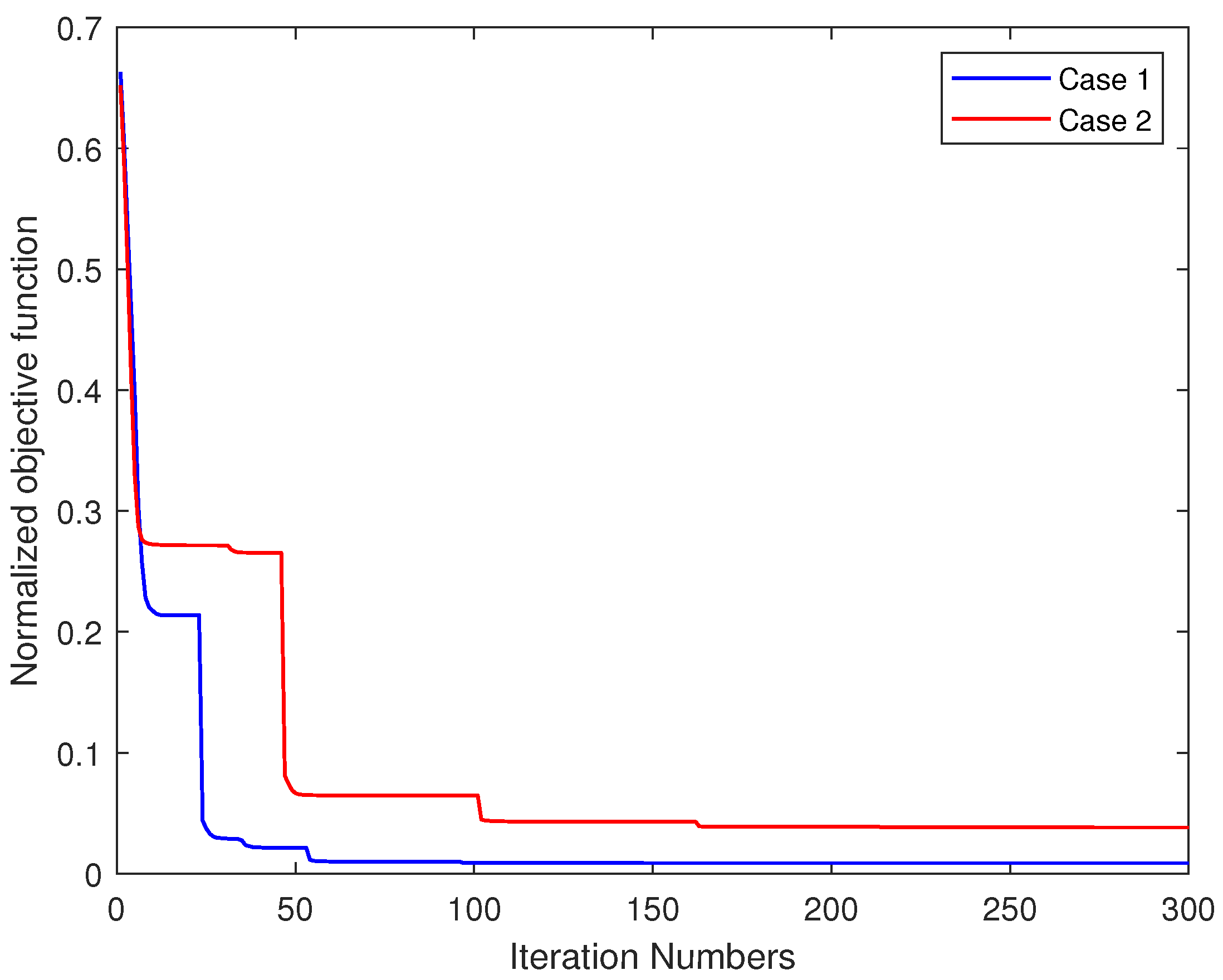
Figure 1 shows normalized objective function versus the iteration numbers with different desired beampatterns. As shown in the figure, when we consider Case 1 as the desired beampattern, the objective function decreases sharply in the first 40 iterations and starts convergence after 150 iterations. When we consider Case 2 as the desired beampattern, the objective function decreases sharply in the first 40 iterations and starts convergence after 110 iterations. Besides, the total computation time when considering Case 1 is 30.2 s, and the total computation time when considering Case 2 is 38.0 s.
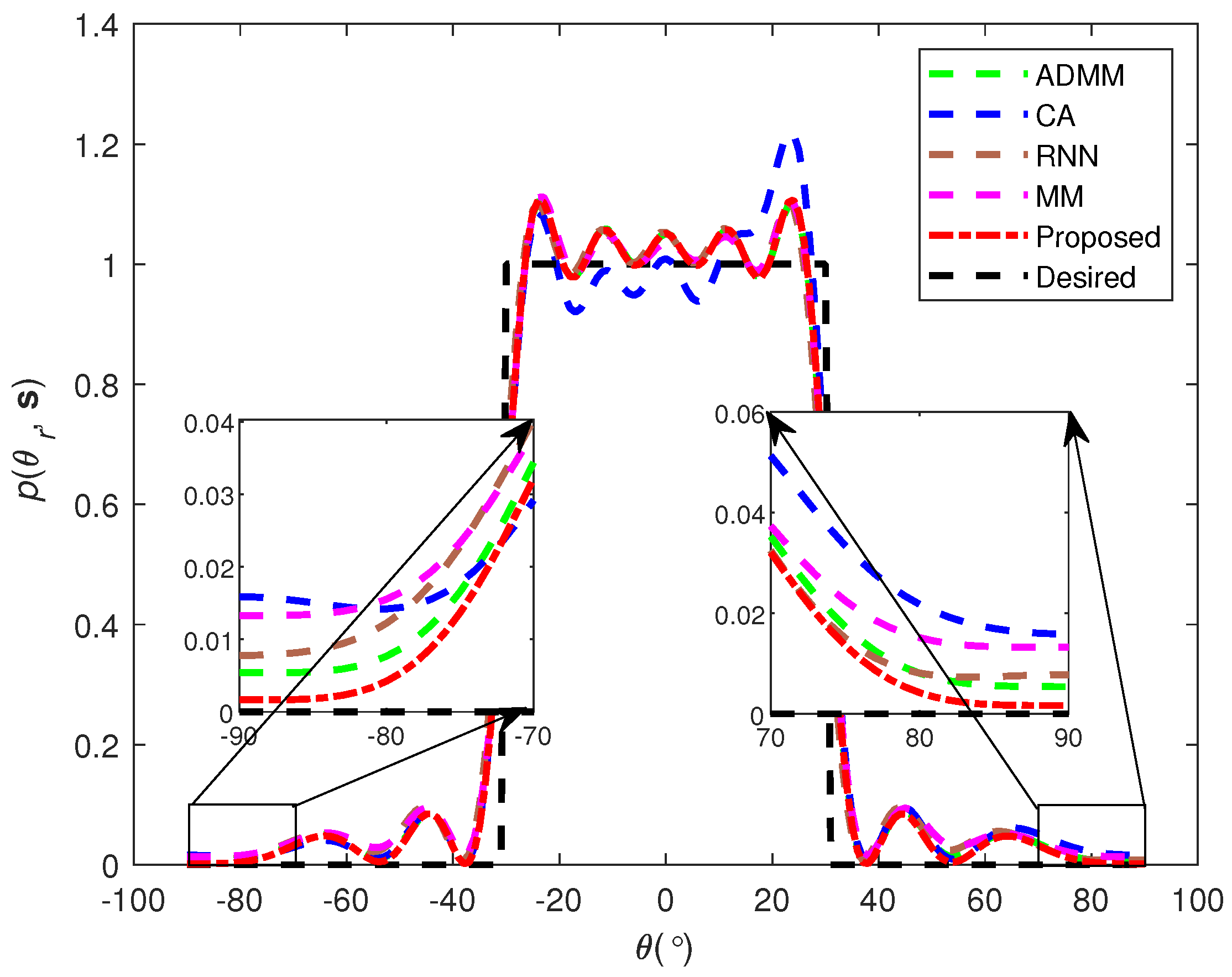
6.2. The Comparison of Beampattern Matching Performance between the Proposed Method and Other Methods
In this subsection, we consider the MM-based method in [
12], the CA method in [
10], the ADMM-based method in [
13], and the RNN method in [
14] for comparison. We further consider Case 1 as the desired beampattern with one mainlobe in
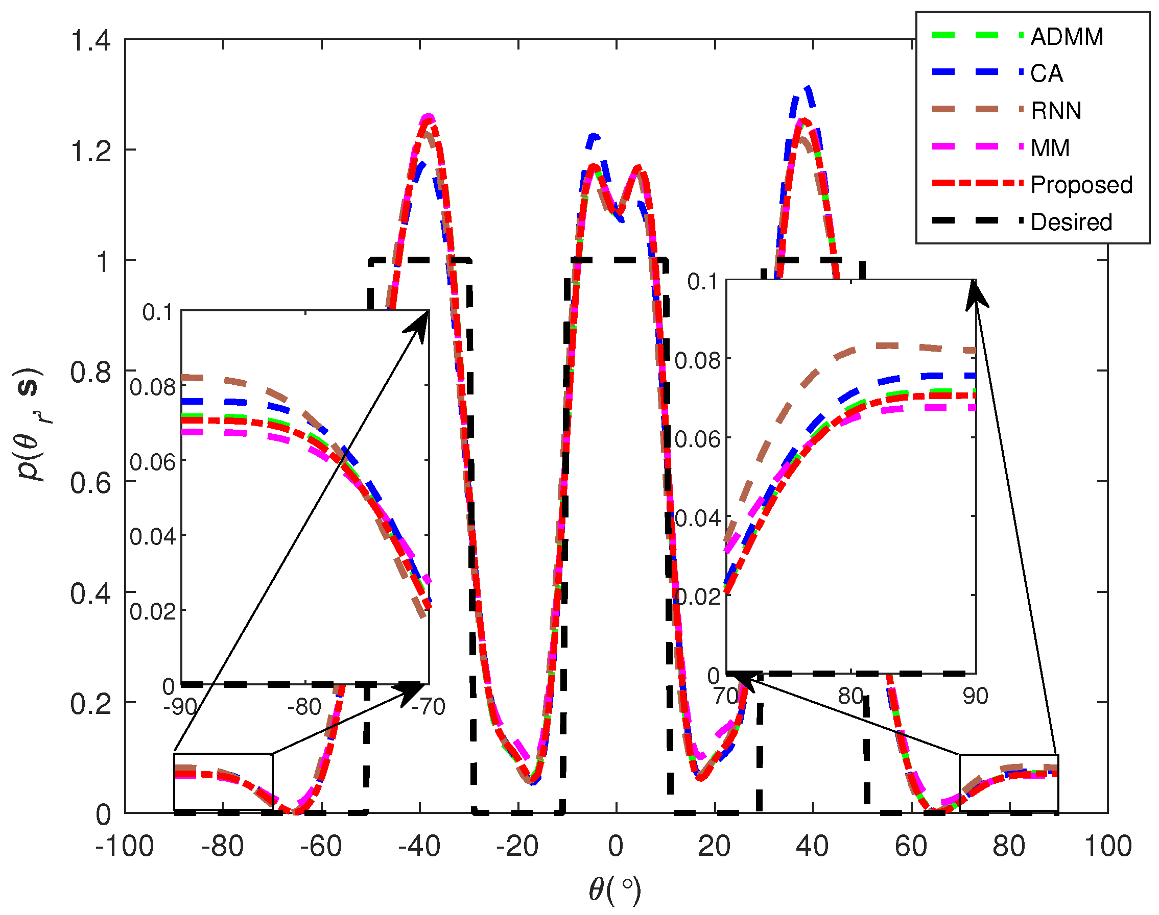
Figure 2 and Case 2 as the desired beampattern with three mainlobes in
Figure 3, respectively.
As can be seen in
Figure 2 and
Figure 3, the beampattern generated by the proposed method has the lowest sidelobe value in whole angle space, meaning that the proposed method has the best sidelobe suppression ability and the highest beampattern matching accuracy.
We further introduce the mean square error (MSE) in (
41) to show the beampattern matching performance between different methods more clearly. The MSE is the square error between the designed beampattern and the desired one. Hence the lower MSE value means better matching performance.
Table 1 and
Table 2 show the MSE,
, computation complexity, and convergence time for different methods when considering Case 1 and Case 2 as the desired beampattern, respectively. As can be seen from the tables, the proposed method has the lowest MSE values and reasonable computation time. Although the MSE values are similar between the ADMM-based method and the proposed method, the ADMM-based method is not strictly CMC. Hence, with relaxation, the method may have a better performance where we introduce
in (
42) to demonstrate it. As can be seen from the tables, the
in the ADMM-based method has a small value (i.e., not strictly CMC), while the value of it is zero (i.e., strictly CMC) in other methods.
The mean square error (MSE) is defined based on [
38]:
where
is the desired waveform and
is the normalized waveform.
The
is defined based on:
where
is the minimum amplitude in the designed waveform, and
is the maximum amplitude in the designed waveform.
6.3. The Capability of the Cross-Correlation Sidelobes Controlling
We consider that
is not zero and Case 2 as the desired beampattern in the following simulations while other simulation parameters keep the same.
Table 3 shows the results of the cross-correlation sidelobes term (i.e.,
in (
5)) under different values of
). As shown in the table, the cross-correlation sidelobes term is minimized when
is not zero. Besides, the optimal performance is obtained when
.
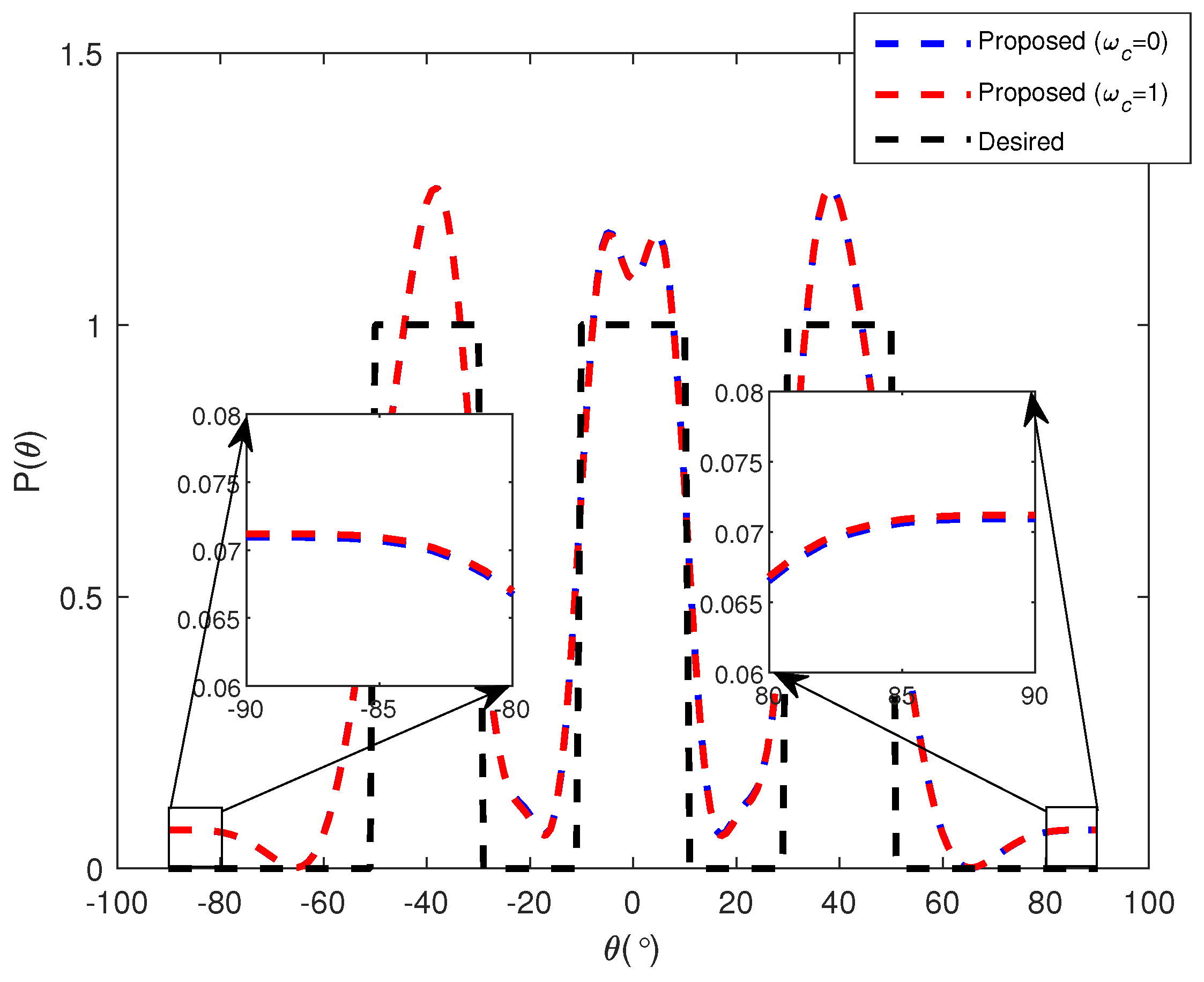
Next, the beampattern matching performance comparison with
and
is illustrated in
Figure 4. The designed beampattern generated considering the cross-correlation sidelobes term (i.e., MSE = 0.0380) is similar to the beampattern obtained without considering the cross-correlation sidelobes term (i.e., MSE = 0.0381), which is because the cross-correlation sidelobes term is quite small compared with the beampattern matching term. Nevertheless, the cross-correlation behavior is much better when using
than that of using
, which is because the generated waveforms under the case of
are almost uncorrelated with each other.
As a result, the proposed method has great cross-correlation sidelobes control capability and can generate uncorrelated waveforms.
6.4. The Performance of the Sparse Beampattern Matching Design
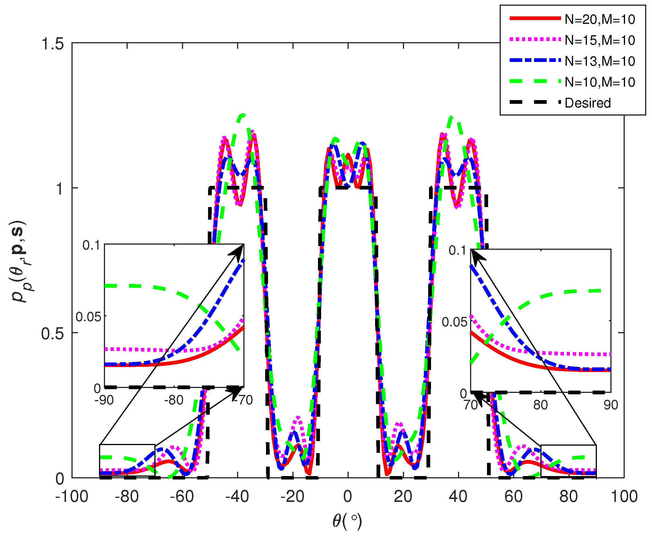
In this subsection, we test the performance of the proposed sparse beampattern matching design method. We consider Case 2 as the desired beampattern with antennas and , 13, 15 and 20 grid points in the following simulations while other simulation parameters keep the same.
Figure 5 shows beampattern matching performance under different numbers of grid points. It can be seen that the sidelobes of the beampattern with sparse antenna positions selection are significantly reduced compared to the beampattern without sparse antenna positions selection (i.e.,
). Besides, as the number of grid points
N increases, the sidelobe values of the designed beampatterns decrease.
Table 4 shows the corresponding MSE values under different numbers of grid points. As can be seen from the table, the MSE values are lower after sparse antenna positions selection and decrease with the increase in the grid points
N, which is consistent with the results shown in
Figure 5. The results shown in
Figure 5 and
Table 4 demonstrate that the proposed sparse beampattern matching design method can greatly enhance the beampattern matching performance by selecting proper sparse antenna positions. Besides, with the increase in the grid points
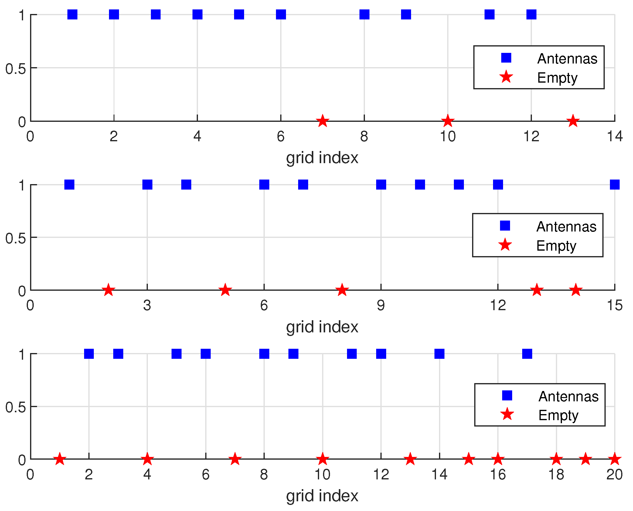
N, more DOF is provided to the system for beampattern designing, which is helpful to increase the beampattern matching performance. Finally,
Figure 6 shows the corresponding sparse antenna positions.
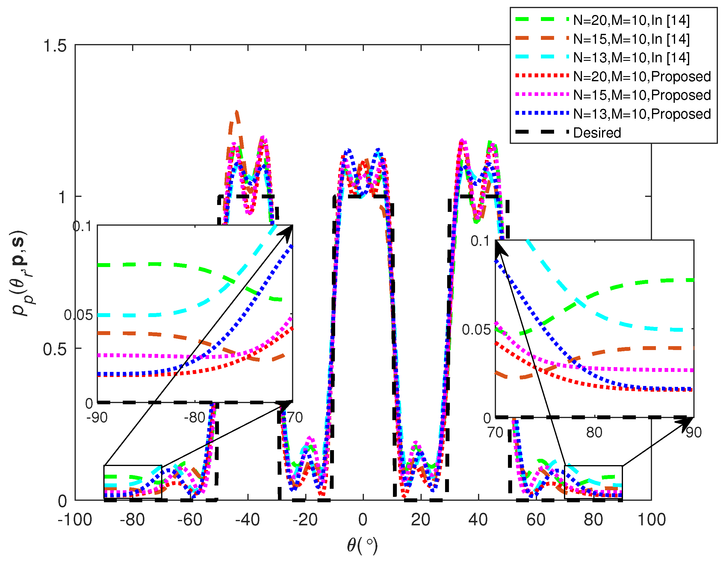
We further compare the proposed method with the method in [
39], which jointly optimize the WCM and the sparse antenna positions. However, the method in [
39] is an indirect optimization method that cannot obtain the waveform directly. To obtain the waveform from the WCM, the CA method in [
10] is used. The result of the beampattern matching comparison between the proposed method and the method in [
39] after the sparse antenna position selection is illustrated in
Figure 7. As shown in the figure, the proposed method has lower sidelobes compared with the method in [
39]. Similar to the above, the comparison in terms of MSE between the two methods is illustrated in
Table 5. As can be seen from the table, the proposed method has lower MSE values compared with the method in [
39]. Therefore, the proposed method has better accuracy in terms of the sparse beampattern matching design than the method in [
39].
7. Conclusions
In this paper, we consider the MIMO radar waveform design for beampattern matching problem. Unlike most existing methods, which approach this challenge by relaxation, the novel optimization method DBMWR is developed without relaxation by noticing the new intrinsic of CMC. More precisely, the problem is first transformed into an unconstraint quartic polynomial over the CC, and, after that, it is solved through the proposed method. Results show that the DBMWR method obtains a balance in terms of computation complexity and accuracy compared with the existing methods.


