Article

Optimal Sample Size and Composition for Crop Classification with Sen2-Agri’s Random Forest Classifier

1
CIMMYT-China Joint Center for Wheat and Maize Improvement, Henan Agricultural University, Zhengzhou 450002, China
2
CIMMYT-Mexico, Sustainable Agrifood Systems Program (SAS), Texcoco 56237, Mexico
3
Lincoln Agritech Ltd., Lincoln University, Christchurch 7674, New Zealand
4
Earth and Life Institute, Université Catholique de Louvain, 1348 Louvain-la-Neuve, Belgium
5
AgroBioSciences Department, Mohammed VI Polytechnic University, Ben Guerir 43150, Morocco
*
Author to whom correspondence should be addressed.
Remote Sens. 2023, 15(3), 608; https://doi.org/10.3390/rs15030608
Submission received: 13 December 2022 / Revised: 12 January 2023 / Accepted: 17 January 2023 / Published: 19 January 2023
(This article belongs to the Collection Sentinel-2: Science and Applications)

Abstract

:
Sen2-Agri is a software system that was developed to facilitate the use of multi-temporal satellite data for crop classification with a random forest (RF) classifier in an operational setting. It automatically ingests and processes Sentinel-2 and LandSat 8 images. Our goal was to provide practitioners with recommendations for the best sample size and composition. The study area was located in the Yaqui Valley in Mexico. Using polygons of more than 6000 labeled crop fields, we prepared data sets for training, in which the nine crops had an equal or proportional representation, called Equal or Ratio, respectively. Increasing the size of the training set improved the overall accuracy (OA). Gains became marginal once the total number of fields approximated 500 or 40 to 45 fields per crop type. Equal achieved slightly higher OAs than Ratio for a given number of fields. However, recall and F-scores of the individual crops tended to be higher for Ratio than for Equal. The high number of wheat fields in the Ratio scenarios, ranging from 275 to 2128, produced a more accurate classification of wheat than the maximal 80 fields of Equal. This resulted in a higher recall for wheat in the Ratio than in the Equal scenarios, which in turn limited the errors of commission of the non-wheat crops. Thus, a proportional representation of the crops in the training data is preferable and yields better accuracies, even for the minority crops.

1. Introduction

The launch of the Sentinel-2 satellites in 2016 and 2017 has opened new avenues for crop identification based on optical satellite data [1]. They acquire multi-spectral data at a ground sampling distance of 10 m and have a revisit frequency of five days at the equator [2]. The resulting time series of images should make it possible to identify crops early in the season and to increase general classification accuracy [3]. Using a time series of images poses a new challenge: the large number of images that need to be handled calls for an automated pre-processing system. Sen2-Agri addresses this need [4]. It can be used to create a cropland mask and, in a second step, identify crop types [5]. Another software tool, called Sentinels for Common Agricultural Policy (Sen4CAP), uses the same random forest (RF) classification engine [6]. The RF algorithm [7] is fast and relatively insensitive to overfitting [8]. Unlike other machine-learning algorithms, RF does not need much finetuning of hyperparameters and can handle simple and complex classification functions [9,10].
Machine-learning algorithms are generally perceived to be data hungry, i.e., the more training data that are available, the better the resulting classification accuracies [11]. Based on expert knowledge, the developers of Sen2-Agri generally recommend that for a given stratum, the user provides 75–100 samples for each main and 20–30 samples for each minor crop [5]. Considering the 75% split of the samples into training and validation pixels, this rule of thumb is close to the 50 sample units (pixels, clusters of pixels, or polygons) per class suggested in other studies [12,13]. However, Congalton [12] also pointed out that conventional statistical approaches to calculate sample sizes based on an approximation of a binominal distribution are only valid to estimate the OA of a single category. They are not appropriate to calculate the error matrix because they do not account for the confusion of specific categories or crop types, as in this study. He concluded that “because of the large number of pixels in a remotely sensed image, traditional thinking about sampling does not often apply” and that a balance between what is statistically sound and what is practically attainable must be found. Another approach has been to define the number of samples needed per class as a function of bands used for the analysis. The general recommendation was to use 10 to 30 times as many samples per discriminating waveband [14]. However, using a machine-learning algorithm in combination with a Monte Carlo analysis for a multi-temporal crop classification, Van Niel et al. [15] established that for their case study, approximately 2 to 4 samples per discriminating waveband were sufficient to attain 95% of the accuracy achieved with 30 samples. They further cautioned that, ultimately, the number of samples needs to be determined by considering the complexity of the discrimination problem. Based on an analysis of a binary classification, Waldner et al. [16] demonstrated that the class proportions of the training data were more important for achieving a high classification accuracy than the sample size.
Apart from government agencies, which use the data to produce crop statistics [17], many other types of organizations collect crop type information. Disaster and relief organizations rely on them for assessing crop production prospects [5]. Policy planners and researchers use them for technology targeting [18] or yield gap analyses for specific crops [19]. The food processing industry tends to be interested in specific crops to forecast the supply of inputs as early as possible and plan the logistics after harvest. Focusing on just one crop versus everything else may also reduce the error rate in the training data. It can be challenging to accurately identify all the crops, especially when doing a wind-shield survey.
Most farming landscapes are dominated by few crops. If the training data are collected in a random manner, the predominant crops will also be strongly represented, whereas fewer fields of the minority crops will be collected [20]. This may, in turn, decrease their classification accuracy, and the training data will most likely be imbalanced as well. The marginal return (in terms of classification accuracy) of adding fields of dominant crop types may diminish rather quickly. It might be better to pay more attention to the less dominant crops to improve their classification accuracy. But this could lead to an overestimation of the crops belonging to a minor class. Millard and Richardson [21] showed how the change in the proportion of training samples affected the classification output and thus introduced errors. Accordingly, Mellor et al. [22] reported that balanced training data, in which the crops have a proportional representation, resulted in the lowest overall error rates. However, they also noted that a sensible correction of imbalance can improve the classification performance for “difficult” classes.
Careful preparation of the in situ data is a prerequisite for successful crop classification. The general rule of thumb for machine learning is that 80–90% of the time is spent preparing the data, and the remainder is used for classification, analysis and interpretation of the results [23]. Hence, guidelines, not only for practitioners but also for researchers, are needed to help them optimize the use of limited resources. Our paper will address the following questions:
  • Does a proportional or equal representation of each crop type in the training data generate better classification results?
  • What is the optimal number of training fields?
  • How does classification accuracy change with time across the season?
  • What kind of accuracies can be achieved with a binary classification, in which one focuses just on one crop vs. “everything else”?
In this paper, we first present the overall workflow (Section 2.1) and then explain how we created the in situ data (Section 2.2). Next, we describe the Sen2-Agri system (Section 2.3) and how we created different scenarios (Section 2.4) and naming conventions (Section 2.5) to answer the above questions. The four questions are then used to structure the Result and Discussion sections.

2. Materials and Methods

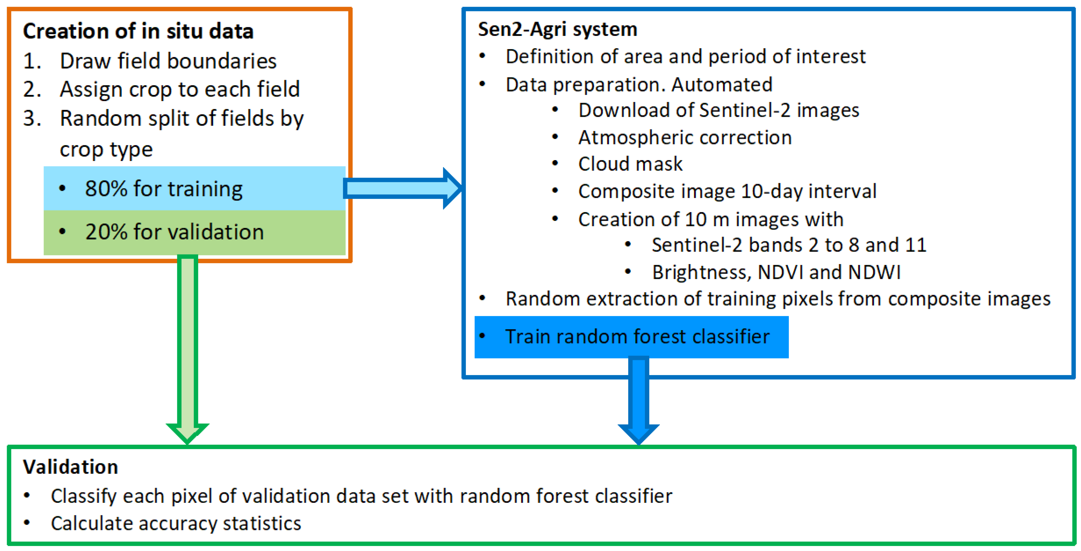
2.1. Overall Workflow

The workflow consisted of three main tasks, as shown in Figure 1:
  • Creation of the in situ data set consisting of more than 6000 crop fields.
  • Running of the Sen2-Agri system to access and process the Sentinel-2 data from the Copernicus Open Access Hub. The RF classifier of Sen2-Agri was then trained with specific input data for the various scenarios described in Section 2.4.
  • Application of the RF classifier to the validation data set to calculate classification accuracies.
Figure 1. Overview of the workflow.
Remotesensing 15 00608 g001

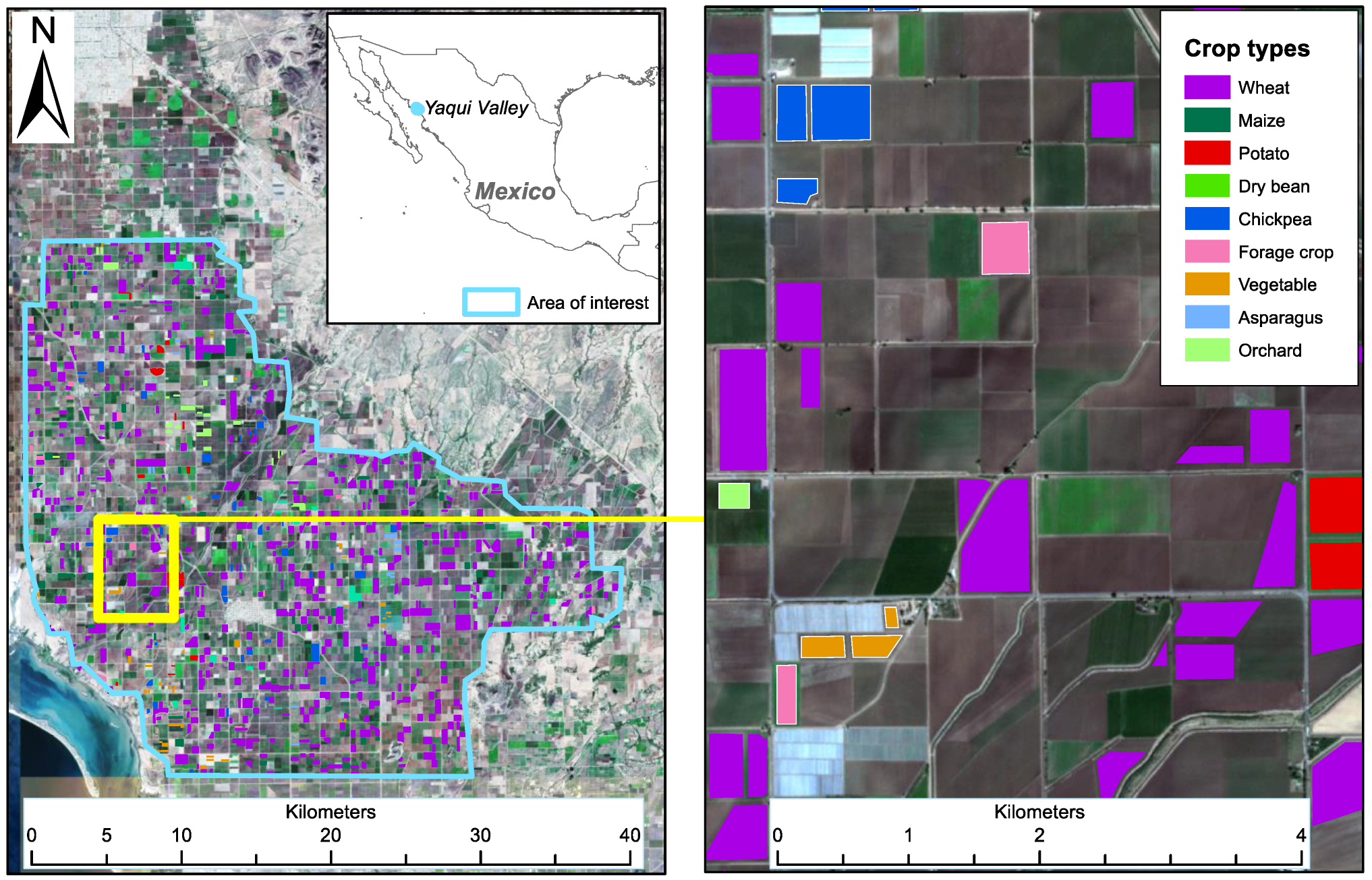
2.2. Characteristics of the Study Region and In Situ Data Preparation

Our study region is located in the Northwest of Mexico, in the Yaqui Valley, where farmers grow crops under irrigated conditions during the winter months. Wheat, the dominant crop, is usually sown between mid-November and mid-December (Table 1). However, some fields are sown as late as early January. Among the other eight crops that will be referred to as minority crops in this study, maize and chickpea were the most important ones. Sen2-Agri was developed with the primary goal of identifying major annual field crops, although we also included some permanent crops such as asparagus, alfalfa and pasture (grassland), as well as tree fruit and nuts, categorized as orchard. Alfalfa and pasture were categorized as forage crop. The fields near the coast showed more variability in the normalized difference vegetation index (NDVI) than those at a further distance, presumably due to elevated levels of soil salinity [24]. However, we did not create an additional stratum for those fields.
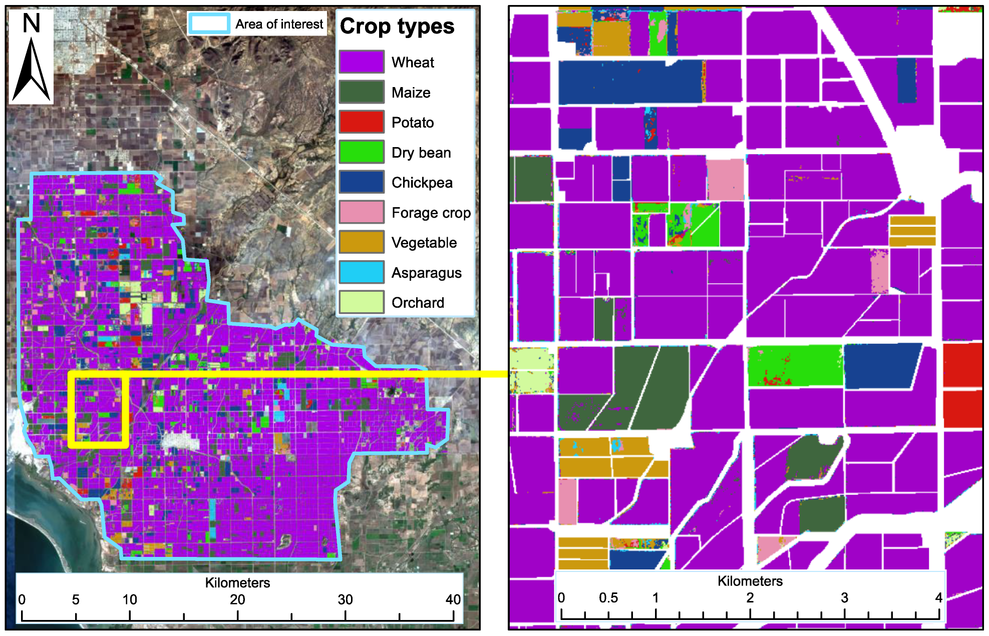
The focus of this study is on the identification of crops within known field boundaries. Therefore, we did not generate a crop mask because any error in the crop mask would have led to the omission of crop or inclusion of non-crop pixels. The planners of the Yaqui Valley irrigation scheme had divided the land into blocks measuring 2 by 2 km. The blocks were further subdivided into 40 lots, each measuring 10 ha. The blocks and lots were numbered consecutively. At the beginning of the winter growing season, the irrigation district, called Distrito del Riego del Rio Yaqui, requires each farmer to declare the type of crop they plan to grow on each irrigated lot. Most farmers do not follow the initial lot boundaries any more. Some lots were split up, whereas most were merged. If farmers had merged several lots, they would use the number of their first lot as an anchor and also report the area of the entire field, i.e., the merged lots, that were planted with the same crop. Based on the farmer’s declarations, which include the crop type, block, lot and field size, the crop types were then assigned to the field boundaries, which had been manually drawn beforehand, using a Sentinel-2 image from 13 March 2017 as a background. This resulted in 6048 labeled fields (Figure 2). The average area of a field was 11.5 ha. Subsequently, they were randomly split into two sets: 80% of the fields of each crop type were set aside for training, and the remaining 20% were used for independent validation of the classifications (Table 2). Thus, all accuracy assessments were conducted against the same set of validation data. To reduce the effects of mixed border pixels, we applied a 1-pixel (10 m) inner buffer to all fields that were used for training but not for validation.
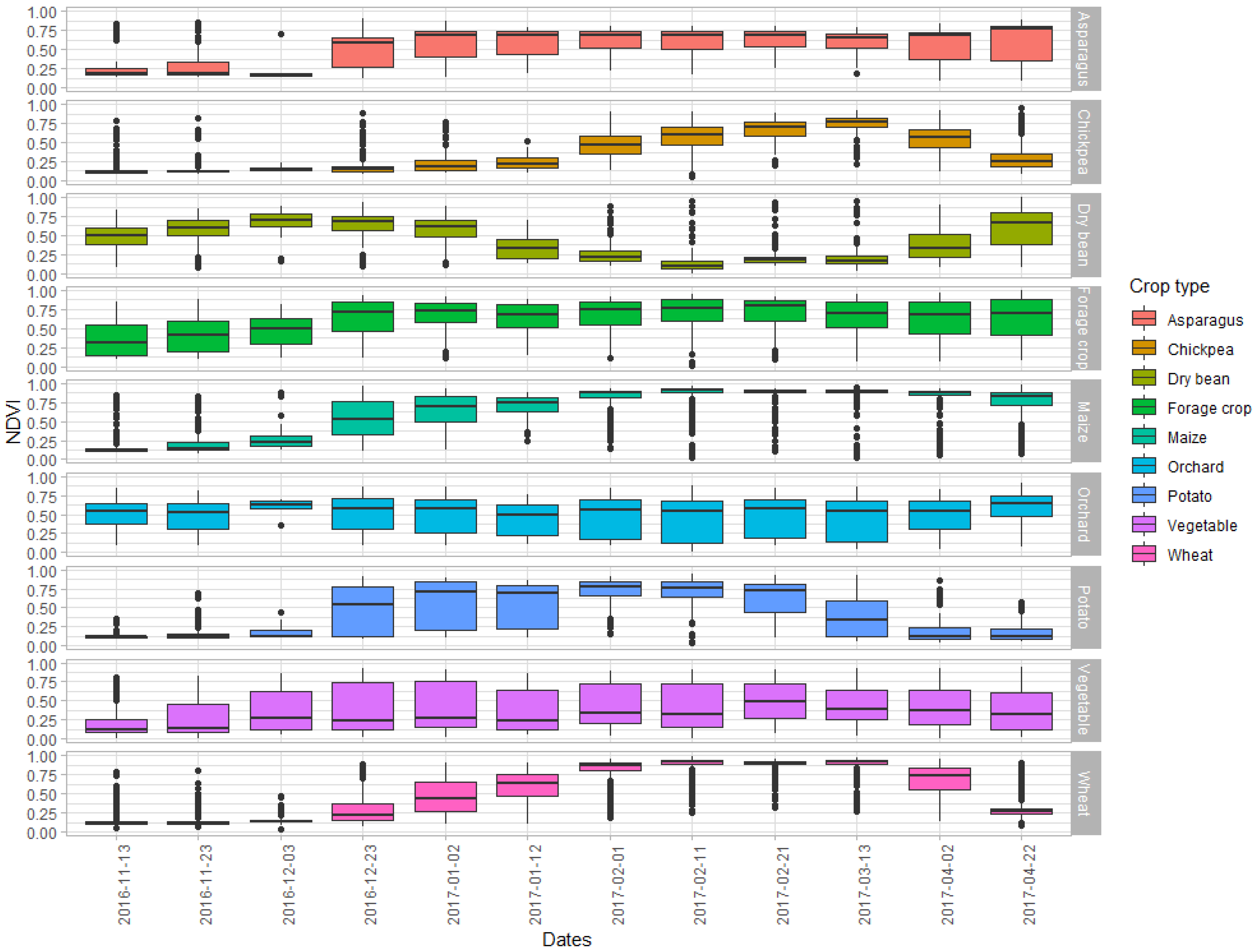
All in all, 12 images, acquired by Sentinel-2A for tile 12RXR between 13 November 2016, and 22 April 2017, could be used for the analysis. The acquisition dates are shown in Figure 3, together with the dynamics of the NDVI [25] of the labeled fields across the growing season.

2.3. Sen2-Agri Crop Classification System

Sen-Agri had been designed to run crop classifications in an operational manner [5]. It automatically downloads the images for a defined area of interest (AOI) or accesses them when set up in a cloud infrastructure; it masks out clouds and shadows and applies an atmospheric correction using the MACCS ATCOR Joint Algorithm (MAJA) [26]. Masked-out pixels are gap filled, based on a linear interpolation between cloud-free pixels of the previous and subsequent image(s). This results in a series of images with a 10-day interval spanning the entire growing season. For the crop classification, Sen2-Agri uses the 10 m bands (2, 3, 4 and 8) of Sentinel-2, the 20 m red-edge bands (5, 6 and 7) and the SWIR band (11), resampled to 10 m. In addition to the surface reflectance of the different bands, Sen2-Agri calculates NDVI, the normalized difference water index (NDWI) [27] and brightness, defined as the Euclidean norm of the surface reflectance values in bands 3, 4, 8 and 11.
For the cropland and crop-type identification, the user needs to supply a shapefile with polygons of the in situ data. If needed, it is possible to stratify the target area to accommodate differences in climate, soil, or management practices. Although Sen2-Agri requires the user to prepare the training data as polygons, it does the crop classification at the pixel level. The in situ data typically represent entire crop fields. Sen2-Agri splits them into a training and a separate, independent validation data set. The default split is 75% of the fields of each crop type for training and 25% for validation. The system then puts all the training pixels into one bag and the validation pixels into another. When drawing the pixels from the training bag, it does not consider the crop type. This implies that the more pixels of a given crop type are provided, the higher its chances of being used for training. Having been developed for practitioners, the Sen2-Agri system is optimized for predefined sequences of operations, and only a few intermediary products are stored to reduce the required storage capacity.
Sen2-Agri can also process 30 m Landsat-8 images. However, we did not include them because the fields of the minority crops tended to be small (Table 1), which would have resulted in many mixed pixels. Relying on a toolbox did not allow us to test the behavior of other classification algorithms, nor could we fine-tune the algorithm by optimizing various parameters.

2.4. Scenarios

To assess the impact of the size and composition of the training data on the resulting classification accuracies, we tested different scenarios:
Scenario 1, called “Ratio”: Different ratios were randomly drawn from the training data set, maintaining the proportional representation of the crop types. Based on the 80% of the fields set aside for training, we tested the following ratios: 0.08, 0.10, 0.12, 0.18, 0.31 and 0.64. Thus, the smallest ratio (0.08) corresponds to 6.4% of the fields and the highest ratio (0.64) to 49.6% of the fields of the study area. Potato with 105, and asparagus with 131 labeled fields, constrained the boundary for the lowest ratio that could be realistically tested. The number of fields available for each crop type and ratio level is listed in Table 2.
Scenario 2, called “Equal”: In this scenario, each crop type was represented by the same number of fields for the training of the classifier. We increased the number of fields by 10, from 10 to 80, resulting in eight levels. For each level, the random selection of the fields was made separately.
Scenario 3, called “In-season”: To determine how early and accurately crops can be identified in the season, we ran Ratio-0.31 over four different periods, at monthly increments. We had picked this ratio for the analysis because the results from Scenario 1 indicated that its classification accuracies were relatively stable and did not fluctuate much. All four periods started in November and ended in January, February, March or April.
Scenario 4, called “Binary in-season classification”: To test the feasibility of focusing on just one crop, we created two classes: (1) crop of interest; in this analysis, this was either maize or wheat, and (2) all other classes merged into a single class, non-maize or non-wheat, respectively. In addition, we wanted to assess how early in the season it would be possible to identify either.

2.5. Nomenclature and Statistical Analyses

We used the following naming convention: a crop classification conducted for a proportional representation of fields is called “Ratio” followed by the fraction of fields used; e.g., “Ratio-0.08” stands for a proportional use of 8% of the fields of each crop type. Likewise, “Equal-10” uses ten fields of each crop type. To smooth out the random variability of the performances of each classifier, the treatments for scenarios Ratio and Equal were run six times. Each run was initiated with a different random seed number.
All classification results reported in this paper are based on the same 20% of fields of each crop type set aside initially for an independent validation of the classifications. We used the standard confusion matrix to summarize the classification accuracies at the pixel level. The following statistical parameters were calculated: precision, recall, F-score and OA [28].

3. Results

3.1. Evolution and Dispersion of Crop-Specific NDVI over Time

The dynamics of NDVI distribution per crop vs. time during the investigation period are shown in Figure 3. The two main crops, wheat and maize, indicate considerable heterogeneity in NDVI during the late December and January period, presumably resulting from a wide range in sowing dates. These two crops had similar NDVI development patterns, although the plateau was more prolonged for maize. Most wheat fields had reached senescence by late April, whereas most maize fields were still green. Forage fields, which are being cut several times during the winter growing season, exhibited a wide range of NDVI throughout the monitoring period. Asparagus, another permanent crop, had low vegetation cover during its main harvest period in November and December. For orchards, the average NDVI remained stable. Most dry bean fields were sown in October and reached maturity in January. However, the graph also shows a few fields that were sown as late as January. Chickpea fields were sown last, in late January. There was considerable spread during the planting and harvest periods among the potato fields. The majority was planted in December and got harvested by March. The vegetable class, which was quite diverse and consisted of different types of tomato, broccoli, pumpkin, salads and others, had no uniform development either.

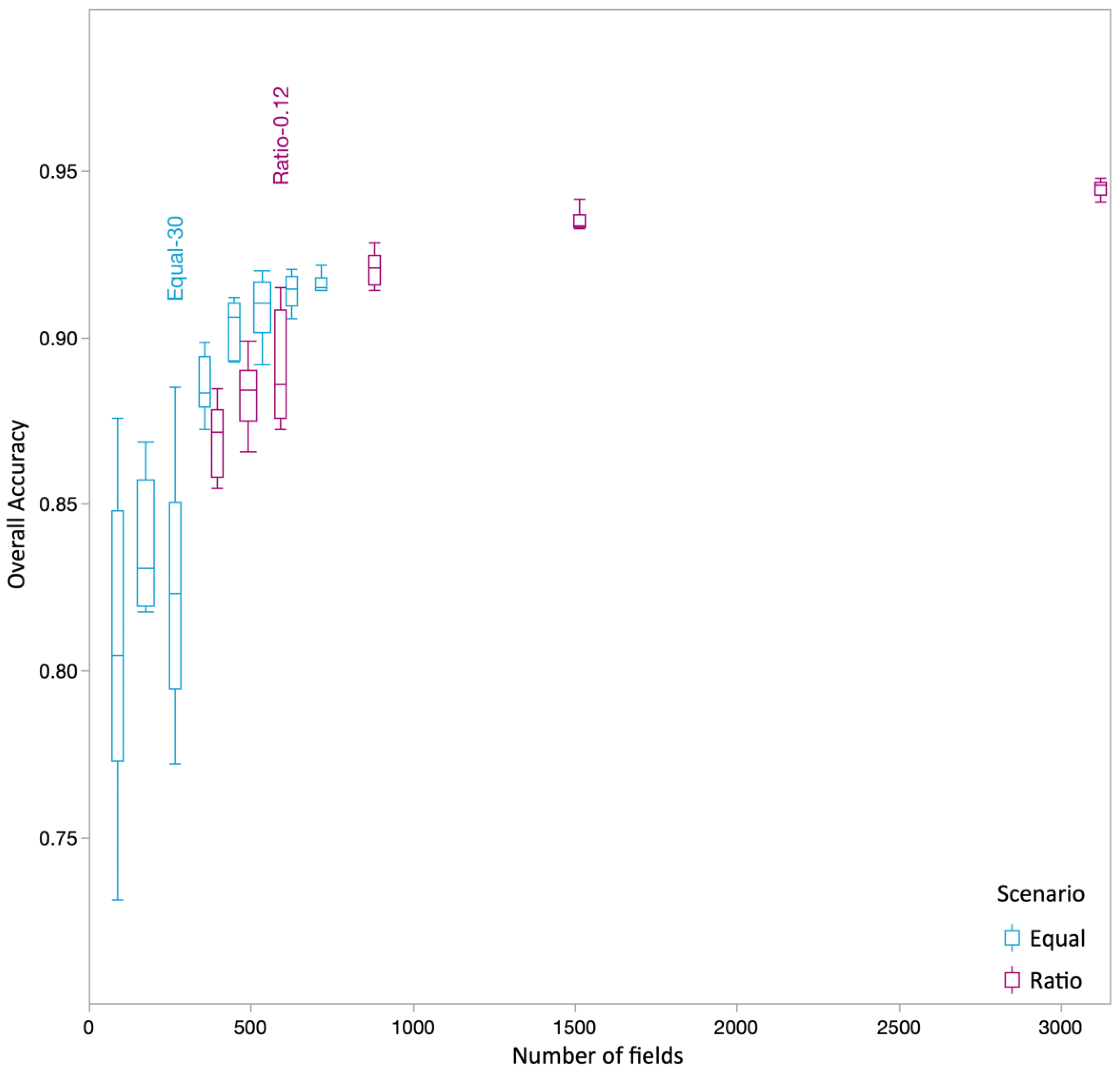
3.2. Classification Results for Ratio and Equal

Our data set allowed us to investigate the limits of accuracy that can be obtained by using a relatively large number of fields for the training of the RF classifier. As expected, using more fields resulted in higher OAs for both Ratio and Equal (Figure 4). The three Ratio treatments with the highest number of fields, Ratio-0.18 (876 fields), Ratio-0.31 (1509 fields) and Ratio-0.64 (3018 fields), achieved a higher OA than the best Equal treatment, which was based on 80 fields per crop or 720 in total. A relatively large range in OAs was observed for the three Equal and Ratio treatments with the lowest number of training fields in their respective categories, indicating unstable classifications. When the number of fields was in a similar range, i.e., 360 to 630, Equal trended higher than Ratio. For Ratio, only a slight improvement was observed when increasing the number of training fields above 876. For Equal, the increase started to level off after 540 fields in total, or 60 fields per crop.
To illustrate the classification challenges, we first compared the results from two scenarios: Ratio-0.18 and Equal-80 (Table 3). They had identical OAs of 0.92. For Equal, this was the highest OA that could be achieved. For Ratio-0.18, 618 wheat fields were used for training, together with a combined total of 258 fields representing the other eight crop types. Their numbers ranged from 15 potato to 52 maize fields (Table 2). This contrasts with 80 fields of each crop type and a total of 720 fields used for Equal. Figure 5 shows the classification results obtained for Ratio-0.18, using a random seed of zero. There were few misclassified pixels within the wheat fields, whereas misclassified pixels were well noticeable within the dry bean fields.
For Ratio-0.18, wheat achieved the highest precision (0.98) and recall (0.96). The high precision indicates that the error of commission was only 2%. Since wheat was the predominant crop, the total of 37,345 pixels misclassified as wheat still caused relatively large errors in the precision of the other crops. It accounted for 87% of the errors in maize and 46% in chickpea, 36% in potato, 35% in forage crop, and 33% in vegetable and asparagus. Pixels misclassified as potato and vegetable also contributed a combined 63% to the classification errors in dry bean, causing a relatively low precision of 0.74. Chickpea achieved the second highest recall (0.90), whereas its precision (0.84) ranked third, after wheat and maize. Forage crop had the lowest precision (0.44) and second lowest recall (0.59). Only vegetable had a lower recall (0.56). Precision of asparagus was also low (0.48), but its recall ranked fourth (0.79). Confusion with wheat, orchard and dry bean was the main cause for its low precision.
For Equal-80, similar results as for Ratio-0.18 were observed. However, a larger number of maize and forage crop pixels were misclassified as wheat, causing a drop in recall of wheat to 0.94, as compared to 0.96 in Ratio. Wheat pixels that were not classified as such were the predominant source of error in the precision of the other crops. They accounted for 96% of the errors in the precision of maize and more than 60% in vegetable, forage crop and chickpea. Another reason for the high percentage contribution of wheat to the error of precision of the minority crops was that among them, fewer pixels got misclassified. In Equal-80, 42,237 pixels got misclassified, whereas, in Ratio-0.18, the number was 55,030. The opposite pattern was observed for the false positive pixels classified as wheat, although the differences between Equal and Ratio were smaller. On average, precision for all minority crops was 0.66 for Ratio and 0.67 for Equal, and recall was 0.72 for Ratio and 0.83 for Equal. The largest improvements in recall of Equal over Ratio were observed for forage crop, potato and chickpea. Chickpea was the only crop with a higher recall in Ratio than in Equal.
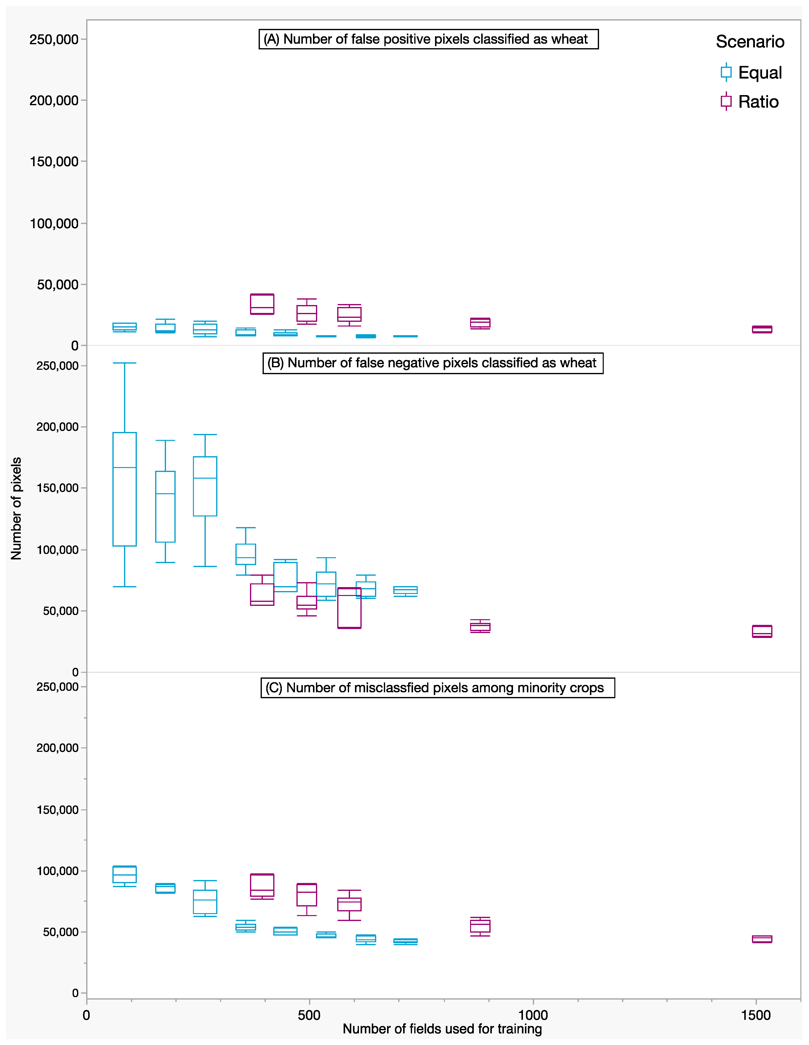
Figure 6 shows that the differences between Equal and Ratio were persistent among all treatment levels. For a given number of fields, the errors of omission (number of false negative pixels) in wheat were larger for Equal than for Ratio. For Equal-10 to 30, the average number was much higher and more variable than for the other scenario levels. On the other hand, Ratio for wheat had a higher number of false positive pixels than the Equal scenarios for a similar number of training fields. When considering only the misclassifications among the minority crops, Equal clearly had fewer misclassifications than Ratio for the range in which the number of training fields was similar.

3.3. How Many Fields Are Needed for Training?

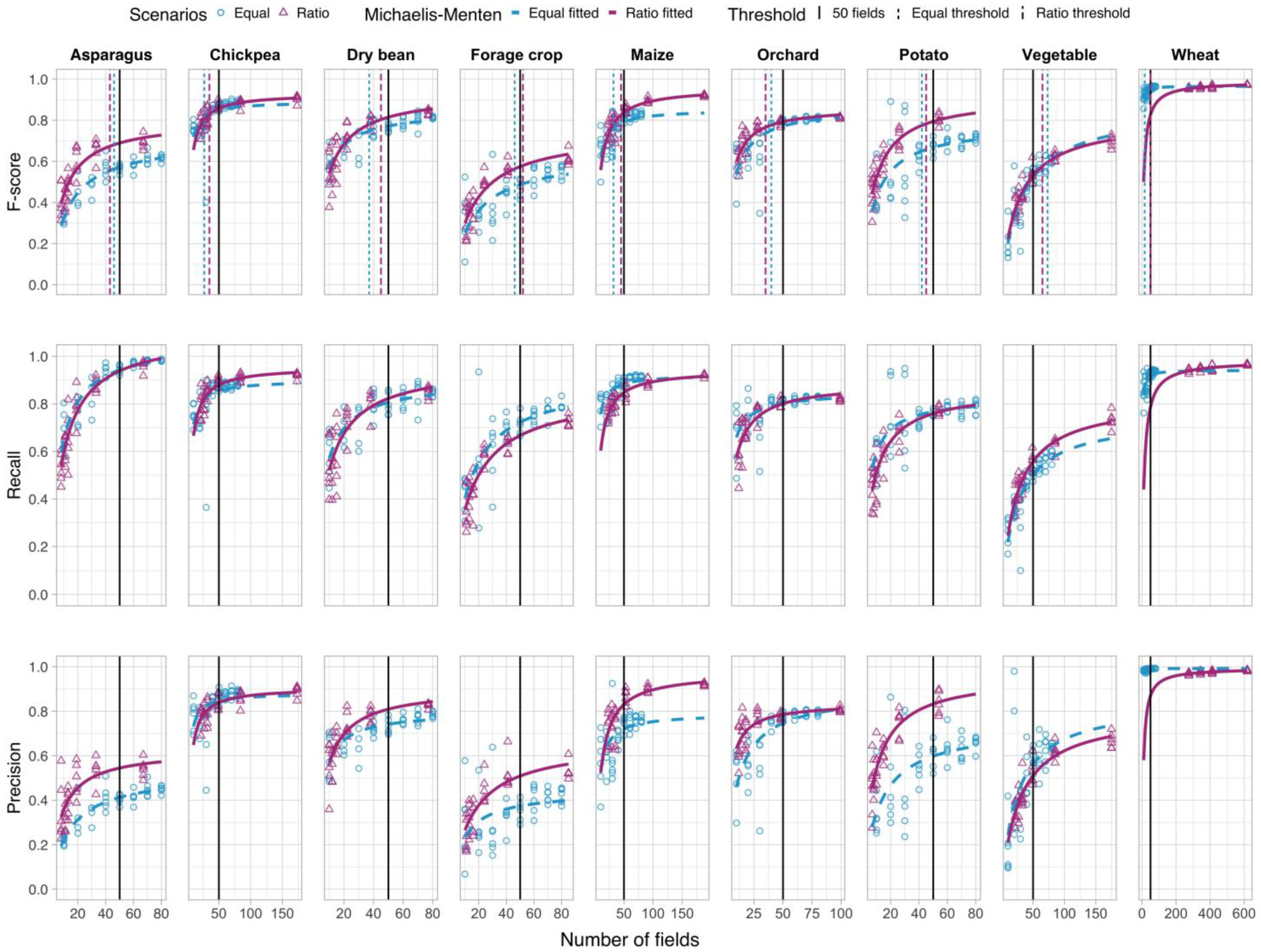
To determine the optimal number of fields required for training, we analyzed the resulting F-score, recall and precision of each crop type (Figure 7) under the Ratio and Equal scenarios. As a breakpoint at which it may not be worthwhile to add more fields to the training data, we set a somewhat arbitrary threshold, at which the increase in the F-scores falls to less than 2.5% for an additional ten fields of a given crop type used for training. A dotted vertical line marks this point in the F-score boxes of Figure 7, where the slope of the first derivative of the Michaelis-Menten curve [29] had declined to 0.0025.
The F-scores indicate that for a given number of training fields per crop type, Ratio tended to perform better than Equal for most crops. Overall, wheat, followed by chickpea, was classified with the highest accuracy. For the Equal treatments of wheat with a low field number, recall tended to range between 0.8 and 0.9. Since wheat represented about 75% of the crop pixels in the study area, an omission error of 10–20% resulted in a large number of misclassified pixels, which in turn decreased the other crops’ precision. For asparagus and dry bean, Equal failed to identify these crops in a total of four instances. The resulting data points with a value of zero were excluded from the fitted Michaelis-Menten curves. Chickpea, forage crop, orchard and potato of the Equal scenario also had a few data points that largely deviated from the fitted curves.
The fitted curves for recall followed similar patterns for Equal and Ratio. The largest difference was observed for vegetables, where Equal did not perform as well as Ratio. Precision of Equal tended to be lower than of Ratio for most crops, except for chickpea, vegetables and wheat.
The impact of adding more fields to the training sets on the F-score leveled off, i.e., the rate of return or increase in accuracy gradually diminished. The threshold of an increase in F-score by 2.5% for an additional ten fields was reached with fewer fields by the Ratio treatment for asparagus, orchard and vegetables. For the other crops, Ratio required more fields than Equal. On average, Equal reached the breakpoint with 40 fields (Std 15.7) and Ratio with 46 fields (Std 9.1). However, the higher average of Ratio was mainly due to wheat.

3.4. Change of Classification Accuracy across the Season

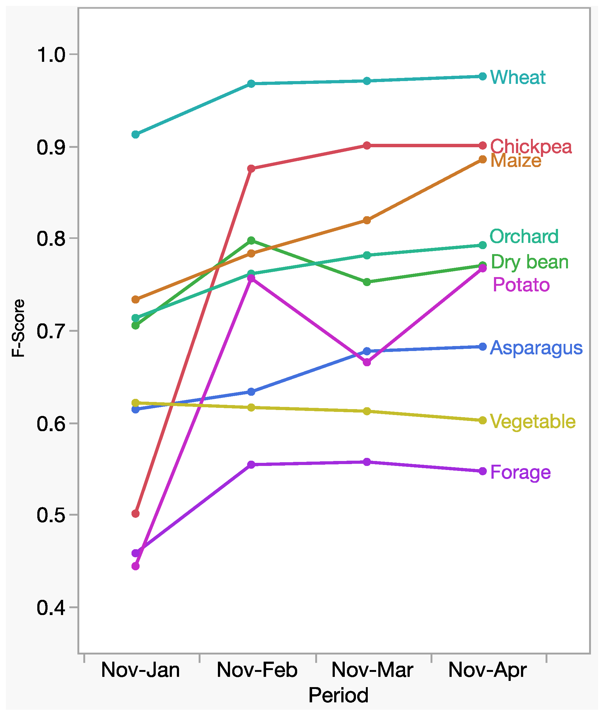
We investigated how the classification accuracies improve over the course of the cropping season by comparing four periods based on the Ratio-0.31 treatment (Figure 8). The results for the first period, November to January, were generally the least accurate in terms of the F-score. The only exception was vegetable, which did not improve over time. The F-scores for wheat (0.97) and forage crops (0.55) had reached a plateau by February, and adding images acquired thereafter did not improve them any further. Maize steadily improved from 0.73 in January to 0.88 in April, whereas orchard increased from 0.71 to 0.79 over the same periods. Potato and dry bean, both of which are harvested in March, saw a drop in the November to March period, as compared to the previous period ending in February.

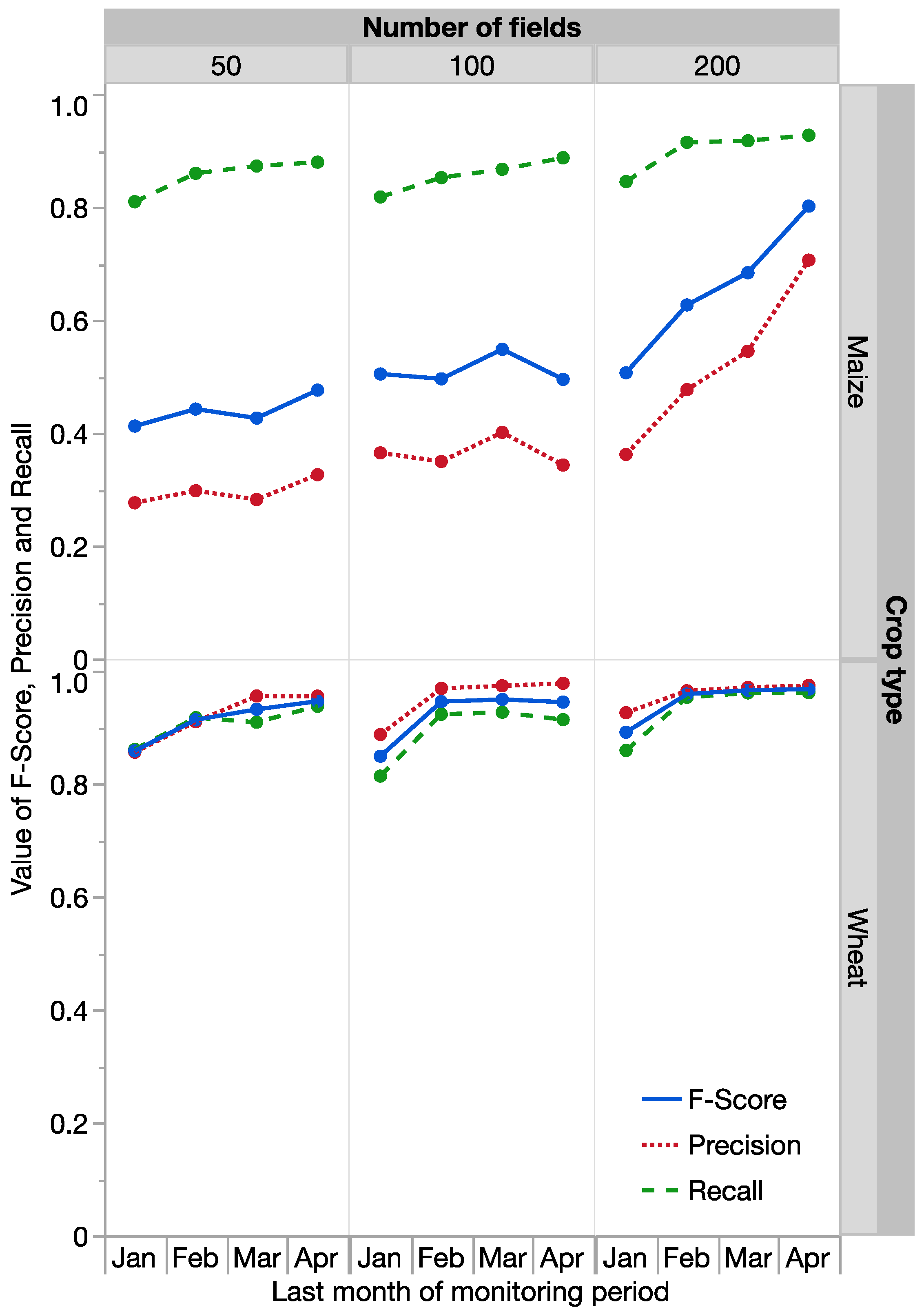
3.5. Binary In-Season Classification

We conducted a similar in-season analysis for the binary scenarios. For maize with 50 and 100 fields, precision remained low throughout the season, but it gradually increased over time for the treatment with 200 fields (Figure 9). However, its recall was above 0.8 in all instances. For wheat, high precision and recall were achieved. Accuracies for the period from November to January tended to be slightly lower than for the longer periods, for which F-scores in the range of 0.91 to 0.97 were observed.

4. Discussion

4.1. Validity of the Study

The large data set allowed us to test different scenarios to identify an optimal sampling strategy for crop classification with an RF classifier. Our study area, located in the Sonora desert, is surrounded by shrubland. Within the irrigation scheme, the land is cropped or used for canals, roads and settlements. Therefore, we did not create a crop mask and limited the training and validation data to pixels located within hand-drawn field boundaries. This omits errors created by a faulty crop mask but may also limit the validity of our study, as Foody [30] recommended considering other land cover types as well when assessing classification accuracies.
Nevertheless, a relatively wide range in sowing dates, elevated soil salinity close to the sea, and inclusion of forage crops and vegetables resulted in diverse conditions (Figure 3). Thus, the findings of this study should be applicable to other crop production regions. Wheat was the predominant crop in our study area. This is the case for many irrigated wheat production regions around the world, where wheat is the only crop widely grown under irrigation during the dry and relatively cloud-free winter months, such as in Egypt, the Indo-Gangetic Plain, or the North China Plain. During the two months of rapid canopy growth between January and February, we had five cloud-free images available to generate the ten-day composite images. This is different from, e.g., Europe or tropical regions during the rainy season, where the creation of composite images based on optical satellites is more challenging [10,31]. The relatively dense series of images may have helped achieve relatively high classification accuracies, some of which were greater than 0.90. They are comparable to results obtained by Sen2-Agri at the country level, with reported OAs in the range of 0.81 to 0.90 [5].
The main source of errors was confusion between wheat and maize. It accounted for a large fraction of the misclassified pixels. After wheat, maize was the second most important crop. Both crops had a similar growth cycle, although maize sowing started earlier and it stayed green for a longer time than wheat did (Figure 3). After wheat, the second highest accuracies were obtained for chickpea, which is sown during a relatively short period in February and has a very well defined NDVI development curve. Since Sen2-Agri had been developed to identify field crops based on spectral time series, it is not surprising that its multi-temporal classification approach works best for field crops with a well-defined sowing window and growth cycle.

4.2. Does Equal or Proportional Representation Produce Better Classification Results?

One of the hypotheses we tested was that minor crops might benefit from a better representation in the training class. Interestingly, in the two lowest Ratio scenarios (Ratio-0.08 and Ratio-0.10), apart from wheat, all crop types were represented by less than 30 fields, yet those two Ratio scenarios achieved higher OAs than Equal-10 to 30. This was due to the fact that in Ratio-0.08 and Ratio-0.10, far fewer wheat pixels in the validation data set were misclassified than in Equal-10 to 30. The F-scores for Equal at a given number of fields were similar but mostly below those of Ratio (Figure 7), except for wheat. For most crops, recall was similar for both scenarios, but precision of Equal was generally lower than for Ratio. This means that in Equal, for the crops other than wheat, a higher percentage of pixels in the validation data set was misclassified due to a higher rate of commission of misclassified wheat pixels, as shown in Figure 6. More wheat pixels did not get classified as such, presumably because fewer wheat fields were used for the training of the Equal than of the Ratio classifier. Thus, the poorer performance of the classifier for the dominant crop caused commission errors for the minor crops. A similar pattern was observed by Jin et al. [32], who reported that proportionally allocated training samples, which corresponds to Ratio in our case, reduced the commission error of the under-represented classes. They further noticed that equally allocated training data helped reduce the omission error of the minority classes. We could observe such a slight reduction for forage crop and maize only.
A training set with proportional data will ensure that the dominant crops are accurately classified and thus reduces the risk that minority crops are confused with them. Mellor et al. [22] and Waldner et al. [16] also advocated that the training data should be representative of their actual proportions in the landscape. If the focus of crop identification is on the minority crops, other sampling approaches [33], and methods to create optimized data sets exist [20]. They have been included in the object-based Sen4CAP open-source system (Sen4CAP, 2021). With Sen2-Agri, a two-stage classification might be an option: In the first step, all crops would have a proportional representation in the training data set. This results in the most accurate classification of the majority crops and reduces their risk of being omitted, which in turn would lead to higher errors of commission in the minority crops. After the fields of the dominant crop(s) have been masked out, the classification could be run again, this time only with the minority crops.

4.3. How Many Fields Are Needed?

The OAs of Equal and Ratio gradually increased with the number of fields used for training to about 0.9 when the impact of adding more training fields leveled off. The high variability of OAs for Equal-10 to Equal-30 fields and for Ratio 0.08 to Ratio 0.12 indicates that the few fields used for training were not fully representative, resulting in highly variable classification accuracies. Our results suggest that a low number of training fields, less than 30 in our study, causes not only low but also unstable classification accuracies. Ultimately, the threshold at which classifications become relatively stable depends on the number of crops and their intrinsic class heterogeneity.
On average, the breakpoint at which an increase in F-score becomes less than 2.5% for an additional ten fields of each crop type was reached at around 40 to 45 fields. Only vegetable required more than 50 fields for Equal and Ratio. That threshold was also surpassed by forage crop and wheat in Ratio. However, the fitted threshold of 51 fields for wheat is lower than the range that had been tested and thus needs to be seen with caution. Our results are in close agreement with the rule of thumb of 50 sample units (pixels, clusters of pixels, or polygons) per class suggested by Congalton [12] and Hay [13]. Their recommendations had been developed before the advent of machine learning but seem to also hold true for the RF classifier. Our recommendation of at least 40 to 45 fields is slightly higher than the 20 to 30 fields suggested for the minority crops by the developers of Sen2-Agri. For the main crops, they suggest using 75 to 100 samples.

4.4. Change of Classification Accuracy across the Season

The test of how early in the season the crops can be identified showed that close to the highest accuracies could be attained by covering the period from November to February, i.e., up to mid-season. As shown in Figure 3, all crops, except for chickpea, had reached their highest NDVI by then. Accordingly, late-season images seem to have a limited impact on improving the classification accuracies of most crops, which is in line with Gilcher [34].

4.5. Binary In-Season Classification

The RF algorithm does not assume a multivariate normal probability distribution of the features [8]. It should, therefore, be suitable for a binary classification, even if one of the classes consists of a mix of all crop types studied. The two binary classification approaches to either identify wheat or maize by grouping all the other crops into one group gave very different results. For maize, the results were poor. But as few as 50 wheat and 50 non-wheat fields resulted in an OA, precision and recall above 0.9. This is remarkable, as it cannot be explained by the unbalanced validation data set alone, which consisted of 75% wheat pixels. Indeed, had the classifier only generated wheat, the resulting map would still have an OA of 0.75, but precision and F-score would be negatively impacted. As shown in Table 3, maize, representing 7% of the cropland, was the crop that was most likely to get confused with wheat. Hence, the signatures of wheat and maize were quite different from the other crops but similar to each other. This explains the results from the maize vs. non-maize classifications. A recall in the range of 0.8 to 0.9 indicates that the algorithm was capable of correctly identifying 80–90% of the maize pixels in the validation data set. But precision was low, in the range of 0.2 to 0.4. This means that many non-maize pixels were identified as maize by mistake, causing an inflated number of pixels labeled as maize. The poor performance of maize in the binary classification is consistent with the results from the comparison between Equal and Ratio: a relatively poor representation of the dominant crop (wheat), as was the case with the Equal scenario in the training set, causes a poor precision of the minority crop (maize).

5. Conclusions

We aimed to generate guidance for the practitioners who are using Sen2-Agri or Sen4Cap in an operational manner. Sen2-Agri can achieve high classification accuracies by the time the crops reach peak NDVI when F-scores higher than 0.95 were obtained for wheat, which was the dominant crop. The test of whether Sen2-Agri is suitable for a binary classification gave mixed results: It worked well for wheat, which dominated the landscape. For maize, a recall above 0.8 could be obtained with only 50 fields, but precision was low. Thus, binary classifications must be carefully examined before applying them at large scales. A proportional representation of the crop types in the data set for training results in better classification accuracies, not only for the dominant crop but also for the minority crops. An accurate classification of the dominant crop reduces the errors of commission for the minority crops. It seems that there is not only an optimal number but also a minimal number of fields that need to be considered for training: Using less than 30 fields yielded unstable results. For the minority crops, the optimal is around 40–45 fields for training, whereas the number for the dominant crops is higher, resulting in a total of around 500 fields. However, additional testing should be done in regions with more than one dominant crop or with frequent cloud cover. Sen2-Agri generates standardized data at a 10-day interval. Hence, it might be possible to apply a classifier developed in one year to images acquired in a different year over the same region. This would be a great step forward toward fully automating crop identification.

Author Contributions

Conceptualization, U.S., F.R., N.B., B.G. and P.D; formal analysis U.S. and F.R.; investigation, U.S., F.R., M.T. and P.D; data curation, U.S., and I.O.-M.; writing—original draft preparation, U.S.; writing—review and editing, U.S., F.R., M.T., S.B., I.O.-M., B.G. and P.D.; funding acquisition, B.G. All authors have read and agreed to the published version of the manuscript.

Funding

This research was funded by the CGIAR Research Program on Maize (www.maize.org) (accessed on 11 December 2022), CGIAR Research Program on Wheat (www.wheat.org) (accessed on 11 December 2022) and Henan Agricultural University.

Data Availability Statement

Schulthess, Urs; Ortiz-Monasterio, Ivan, 2021, “Crop types of the Yaqui Valley during the 2016–2017 winter growing season”, https://hdl.handle.net/11529/10548637 CIMMYT Research Data & Software Repository Network, V1 (accessed on 11 December 2022).

Acknowledgments

We thank the Distrito del Riego del Rio Yaqui for providing the in-situ data and CS Romania for their technical support.

Conflicts of Interest

The authors declare no conflict of interest.

References

  1. Immitzer, M.; Vuolo, F.; Atzberger, C. First Experience with Sentinel-2 Data for Crop and Tree Species Classifications in Central Europe. Remote Sens. 2016, 8, 166. [Google Scholar] [CrossRef]
  2. European Space Agency Sentinel-2 MSI. Available online: https://earth.esa.int/web/sentinel/user-guides/sentinel-2-msi (accessed on 11 December 2022).
  3. Vuolo, F.; Neuwirth, M.; Immitzer, M.; Atzberger, C.; Ng, W.-T. How Much Does Multi-Temporal Sentinel-2 Data Improve Crop Type Classification? Int. J. Appl. Earth Obs. Geoinf. 2018, 72, 122–130. [Google Scholar] [CrossRef]
  4. Sentinel-2 for Agriculture. Available online: http://www.esa-sen2agri.org (accessed on 13 December 2022).
  5. Defourny, P.; Bontemps, S.; Bellemans, N.; Cara, C.; Dedieu, G.; Guzzonato, E.; Hagolle, O.; Inglada, J.; Nicola, L.; Rabaute, T.; et al. Near Real-Time Agriculture Monitoring at National Scale at Parcel Resolution: Performance Assessment of the Sen2-Agri Automated System in Various Cropping Systems around the World. Remote Sens. Environ. 2019, 221, 551–568. [Google Scholar] [CrossRef]
  6. The Sentinels for Common Agricultural Policy-Sen4CAP. Available online: http://esa-sen4cap.org (accessed on 11 December 2022).
  7. Breiman, L. Random Forests. Mach. Learn. 2001, 45, 5–32. [Google Scholar] [CrossRef] [Green Version]
  8. Belgiu, M.; Drăguţ, L. Random Forest in Remote Sensing: A Review of Applications and Future Directions. ISPRS J. Photogramm. Remote Sens. 2016, 114, 24–31. [Google Scholar] [CrossRef]
  9. Sheykhmousa, M.; Mahdianpari, M.; Ghanbari, H.; Mohammadimanesh, F.; Ghamisi, P.; Homayouni, S. Support Vector Machine Versus Random Forest for Remote Sensing Image Classification: A Meta-Analysis and Systematic Review. IEEE J. Sel. Top. Appl. Earth Obs. Remote Sens. 2020, 13, 6308–6325. [Google Scholar] [CrossRef]
  10. Ghassemi, B.; Dujakovic, A.; Żółtak, M.; Immitzer, M.; Atzberger, C.; Vuolo, F. Designing a European-Wide Crop Type Mapping Approach Based on Machine Learning Algorithms Using LUCAS Field Survey and Sentinel-2 Data. Remote Sens. 2022, 14, 541. [Google Scholar] [CrossRef]
  11. Elmes, A.; Alemohammad, H.; Avery, R.; Caylor, K.; Eastman, J.R.; Fishgold, L.; Friedl, M.A.; Jain, M.; Kohli, D.; Laso Bayas, J.C.; et al. Accounting for Training Data Error in Machine Learning Applied to Earth Observations. Remote Sens. 2020, 12, 1034. [Google Scholar] [CrossRef] [Green Version]
  12. Congalton, R.G. A Review of Assessing the Accuracy of Classifications of Remotely Sensed Data. Remote Sens. Environ. 1991, 37, 35–46. [Google Scholar] [CrossRef]
  13. Hay, A.M. Sampling Designs to Test Land-Use Map Accuracy. Photogramm. Eng. 1979, 5, 529–533. [Google Scholar]
  14. Mather, P.M.; Koch, M. Computer Processing of Remotely-Sensed Images: An Introduction; John Wiley & Sons: Hoboken, NJ, USA, 2011. [Google Scholar]
  15. Van Niel, T.; Mcvicar, T.; Datt, B. On the Relationship between Training Sample Size and Data Dimensionality: Monte Carlo Analysis of Broadband Multi-Temporal Classification. Remote Sens. Environ. 2005, 98, 468–480. [Google Scholar] [CrossRef]
  16. Waldner, F.; Jacques, D.C.; Löw, F. The Impact of Training Class Proportions on Binary Cropland Classification. Remote Sens. Lett. 2017, 8, 1122–1131. [Google Scholar] [CrossRef] [Green Version]
  17. Johnson, D.M. Using the Landsat Archive to Map Crop Cover History across the United States. Remote Sens. Environ. 2019, 232, 111286. [Google Scholar] [CrossRef]
  18. Krupnik, T.J.; Schulthess, U.; Ahmed, Z.U.; McDonald, A.J. Sustainable Crop Intensification through Surface Water Irrigation in Bangladesh? A Geospatial Assessment of Landscape-Scale Production Potential. Land Use Policy 2017, 60, 206–222. [Google Scholar] [CrossRef] [PubMed] [Green Version]
  19. Schulthess, U.; Timsina, J.; Herrera, J.M.; McDonald, A. Mapping Field-Scale Yield Gaps for Maize: An Example from Bangladesh. Field Crops Res. 2013, 143, 151–156. [Google Scholar] [CrossRef] [Green Version]
  20. Waldner, F.; Chen, Y.; Lawes, R.; Hochman, Z. Needle in a Haystack: Mapping Rare and Infrequent Crops Using Satellite Imagery and Data Balancing Methods. Remote Sens. Environ. 2019, 233, 111375. [Google Scholar] [CrossRef]
  21. Millard, K.; Richardson, M. On the Importance of Training Data Sample Selection in Random Forest Image Classification: A Case Study in Peatland Ecosystem Mapping. Remote Sens. 2015, 27, 8489–8515. [Google Scholar] [CrossRef] [Green Version]
  22. Mellor, A.; Boukir, S.; Haywood, A.; Jones, S. Exploring Issues of Training Data Imbalance and Mislabelling on Random Forest Performance for Large Area Land Cover Classification Using the Ensemble Margin. ISPRS J. Photogramm. Remote Sens. 2015, 105, 155–168. [Google Scholar] [CrossRef]
  23. Whang, S.E.; Lee, J.-G. Data Collection and Quality Challenges for Deep Learning. Proc. VLDB Endow. 2020, 13, 3429–3432. [Google Scholar] [CrossRef]
  24. Eichler, S.E.; Kline, K.L.; Ortiz-Monasterio, I.; Lopez-Ridaura, S.; Dale, V.H. Rapid Appraisal Using Landscape Sustainability Indicators for Yaqui Valley, Mexico. Environ. Sustain. Indic. 2020, 6, 100029. [Google Scholar] [CrossRef]
  25. Rouse, J.W.; Haas, R.H.; Scell, J.A.; Deering, D.W.; Harlan, J.C. Monitoring the Vernal Advancement of Retrogradiation of Natural Vegetation; NASA/GSFC Type III: Greenbelt, MD, USA, 1974; p. 371. [Google Scholar]
  26. Hagolle, O.; Huc, M.; Desjardins, C.; Auer, S.; Richter, R. MAJA Algorithm Theoretical Basis Document; CNES: Paris, France; CESBIO: Toulouse, France; DLR: Cologne, France, 2017. [Google Scholar] [CrossRef]
  27. Gao, B. NDWI--A Normalized Difference Water Index for Remote Sensing of Vegetation Liquid Water from Space. Remote Sens. Environ. 1996, 58, 257–266. [Google Scholar] [CrossRef]
  28. Foody, G.M. Status of Land Cover Classification Accuracy Assessment. Remote Sens. Environ. 2002, 80, 185–201. [Google Scholar] [CrossRef]
  29. Michaelis, L.; Menten, M.L. Die Kinetik Der Invertinwirkung. Biochem Z 1913, 49, 352. [Google Scholar]
  30. Foody, G.M. Impacts of Ignorance on the Accuracy of Image Classification and Thematic Mapping. Remote Sens. Environ. 2021, 259, 112367. [Google Scholar] [CrossRef]
  31. Orynbaikyzy, A.; Gessner, U.; Conrad, C. Spatial Transferability of Random Forest Models for Crop Type Classification Using Sentinel-1 and Sentinel-2. Remote Sens. 2022, 14, 1493. [Google Scholar] [CrossRef]
  32. Jin, H.; Stehman, S.V.; Mountrakis, G. Assessing the Impact of Training Sample Selection on Accuracy of an Urban Classification: A Case Study in Denver, Colorado. Int. J. Remote Sens. 2014, 35, 2067–2081. [Google Scholar] [CrossRef]
  33. Fowler, J.; Waldner, F.; Hochman, Z. All Pixels Are Useful, but Some Are More Useful: Efficient in Situ Data Collection for Crop-Type Mapping Using Sequential Exploration Methods. Int. J. Appl. Earth Obs. Geoinf. 2020, 91, 102114. [Google Scholar] [CrossRef]
  34. Gilcher, M.; Ruf, T.; Emmerling, C.; Udelhoven, T. Remote Sensing Based Binary Classification of Maize. Dealing with Residual Autocorrelation in Sparse Sample Situations. Remote Sens. 2019, 11, 2172. [Google Scholar] [CrossRef]
Figure 2. Overview of the study area located in the Yaqui Valley, Sonora, Mexico. The background imagery is a Sentinel-2 scene from 23 December 2016, displayed as red, green and blue. Within the area of interest, the boundaries of 6084 crop fields have been manually digitized. On the left side, the 876 fields are shown that were used to train the random forest classifier for the scenario Ratio-0.18, with a random seed of 0. The right side offers a more detailed view of the training and other crop fields.
Remotesensing 15 00608 g002
Figure 3. Development of NDVI of the major crop types across the growing season. The dates indicate the acquisition dates of the cloud-free Sentinel-2A images during the study period.
Remotesensing 15 00608 g003
Figure 4. Overall accuracy (OA) as a function of the number of fields used for training the classification algorithm. Data illustrate two scenarios: For Equal, each crop type was represented with the same number of fields. For Ratio, fields were represented proportionately. Box plots indicate OAs resulting from 6 random selections of training data.
Remotesensing 15 00608 g004
Figure 5. Maps depicting the classification results obtained for the winter 2016–2017 growing season in the Yaqui Valley, Sonora, Mexico. The results represent the scenario Ratio-0.18, with a random seed of zero. The overview map on the left shows that the area of interest was dominated by wheat, covering about 75%. The right side shows the detailed classification results at the pixel level.
Remotesensing 15 00608 g005
Figure 6. Effect of the number of fields used in the set of training data and scenario, Equal or Ratio, on the number of false positive (A) and false negative (B) pixels in the validation data set classified as wheat. The number of misclassified pixels among the non-wheat crops is shown in (C). Box plots represent results from six random selections of training data for each classification scenario.
Remotesensing 15 00608 g006
Figure 7. F-score, recall and precision of nine crop types as a function of number of fields and sampling strategy. Either a fixed or a proportionate number of fields of each crop type was selected for the training set. The respective scenarios are called Equal or Ratio. The solid vertical bar marks 50 fields. The number of fields at which the threshold of an increase in F-score by 2.5% for an additional ten fields was reached is also marked. All classification scenarios were run six times.
Remotesensing 15 00608 g007
Figure 8. F-scores obtained for crop classifications spanning four different periods: The first ranged from November to January and the last from November to April.
Remotesensing 15 00608 g008
Figure 9. Classification accuracy in terms of F-Score, precision and recall resulting from a binary classification of either maize vs. all other crops or wheat vs. all other crops. The classifications were based on 50, 100 or 200 fields representing each class (maize vs. non-maize; wheat vs. non-wheat). Classifications spanned four different periods, ranging from November to January, February, March or April.
Remotesensing 15 00608 g009
Table 1. Summary of the labeled in situ data generated for the crop classification study in the Yaqui Valley (Mexico) for the 2016–2017 growing season. The table shows the average area in hectares (ha) and standard deviation (Std) of the fields of each crop type, as well as the growing period.
CroptypeNumber of FieldsAreaSeasonRemarks
haStdStartEnd
Wheat429112.48.6NovemberApril/May
Maize36613.89.7October/JanuaryApril/JuneAnytime (>120 day crop)
Potato10511.39.5NovemberMarch
Dry bean15111.19.0OctoberMayAnytime (90 day crop)
Chickpea33811.98.9JanuaryMay
Forage crop1667.36.2Perennial
Vegetable3434.62.8OctoberMayAnytime (~90 day crop)
Asparagus1315.32.6Perennial
Orchard1938.87.1Perennial
Total6084
Table 2. Number of fields per crop type used for validation and calibration, as well as for the six ratios (Scenario 1).
CropTotal Number of Fields20% for Validation80% for CalibrationRatio
0.640.310.180.120.10.08
Wheat4291858343321281064618412343275
Maize366732931829153352923
Potato10521845226151087
Dry bean15130121753722141210
Chickpea338682701688449322722
Forage crop16633133824124161311
Vegetable343692741708549332722
Asparagus1312610565321913108
Orchard19339154964828191512
Total60841217486730181509876584487389
Table 3. Classification matrix resulting from using either 18% of the fields (Ratio-0.18) or 80 fields (Equal-80) of each crop type to train the random forest classifier in Sen2-Agri. The data represent the averages obtained from six classification runs initiated with different random seed numbers.
Use of 18% of Fields of Each Crop Type for Training (Ratio-0.18)
ClassifiedReferenceTotal PixelsPrecision
WheatMaizePotatoDry BeanChickpeaForage CropVegetableAsparagusOrchard
Wheat1,021,79811,9401108302104124221341731261,040,1500.98
Maize11,60284,461271041637094791703397,7480.86
Potato270810412,139961128058016941364719,6470.62
Dry bean743694296923,712180573229545941832,0430.74
Chickpea6752628120673377,5451133278744694292,1710.84
Forage crop531065013741430117211,9081732653296527,1930.44
Vegetable4623711149918971855120615,193471160529,0600.52
Asparagus3850619792016127271076010,702220822,2150.48
Orchard17572515516591971100185640727,06735,0240.77
Total pixels1,059,143100,05920,45632,81386,47820,24227,13513,51535,4101,395,251
Recall0.960.840.590.720.900.590.560.790.76
Overall Accuracy: 0.92
Use of 80 Fields of Each Crop Type for Training (Equal-80)
ClassifiedReferenceTotal PixelsPrecision
WheatMaizePotatoDry BeanChickpeaForage CropVegetableAsparagusOrchard
Wheat992,35552125127747980868801001,000,2290.99
Maize27,55691,3124403972024401119,9150.76
Potato28468816,1135803082287154714124,5830.66
Dry bean643654292327,74619223125752441035,3960.78
Chickpea663137122821676,3861242055417986,1310.89
Forage crop14,78711204251085136016,05223807363937,9210.42
Vegetable584829593291151138715,7612439124,6000.64
Asparagus642485712512231431736102713,267439129,4800.45
Orchard205515234155719998978608529,35936,9960.79
Total pixels1,059,143100,05920,45632,81386,47820,24227,13513,51535,4101,395,251
Recall0.940.910.790.850.880.790.580.980.83
Overall Accuracy: 0.92
Disclaimer/Publisher’s Note: The statements, opinions and data contained in all publications are solely those of the individual author(s) and contributor(s) and not of MDPI and/or the editor(s). MDPI and/or the editor(s) disclaim responsibility for any injury to people or property resulting from any ideas, methods, instructions or products referred to in the content.

