
Drivers or Pedestrians, Whose Dynamic Perceptions Are More Effective to Explain Street Vitality? A Case Study in Guangzhou


Abstract
:1. Introduction
1.1. Context
1.2. Research Gap
1.3. Research Question & Hypothesis
2. Literature Review
2.1. Lack of Dynamic Measure of Perception
2.2. Lack of Comparison between Dynamic Perceptions by Modes
2.3. Vitality Can Be under the Influence of Dynamic Perception as Well
3. Data and Method
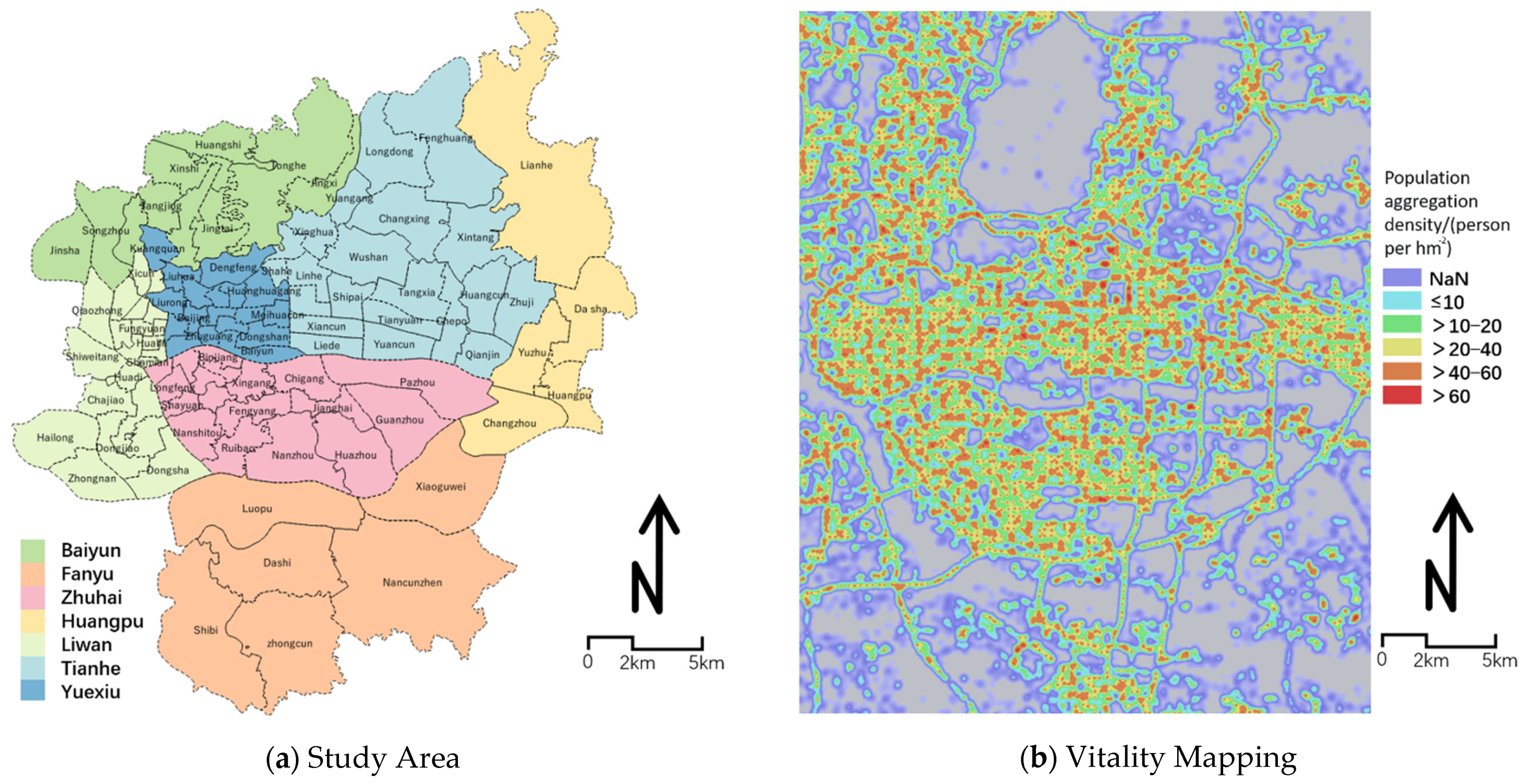
3.1. Study Area
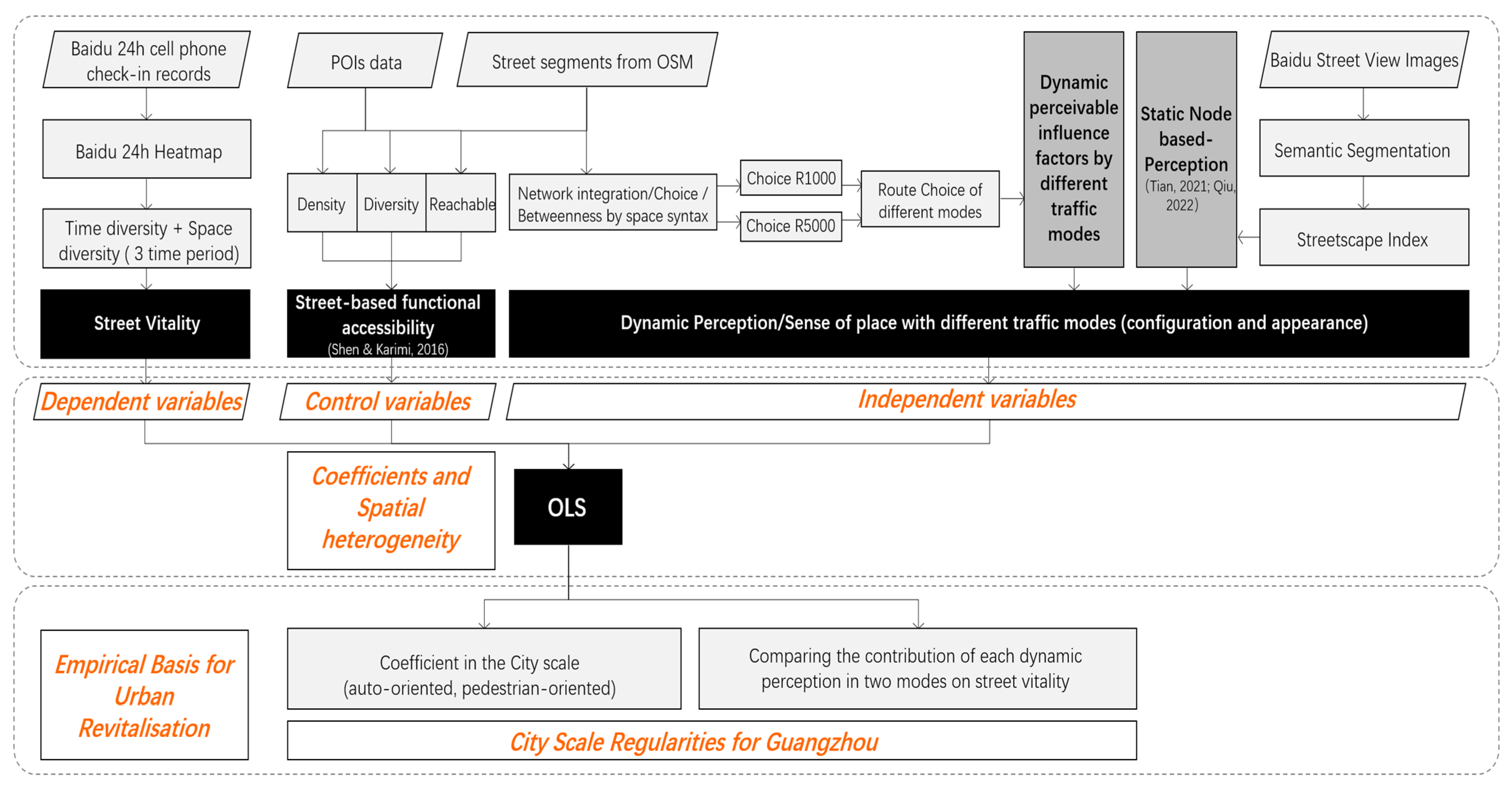
3.2. Analytical Framework and Data
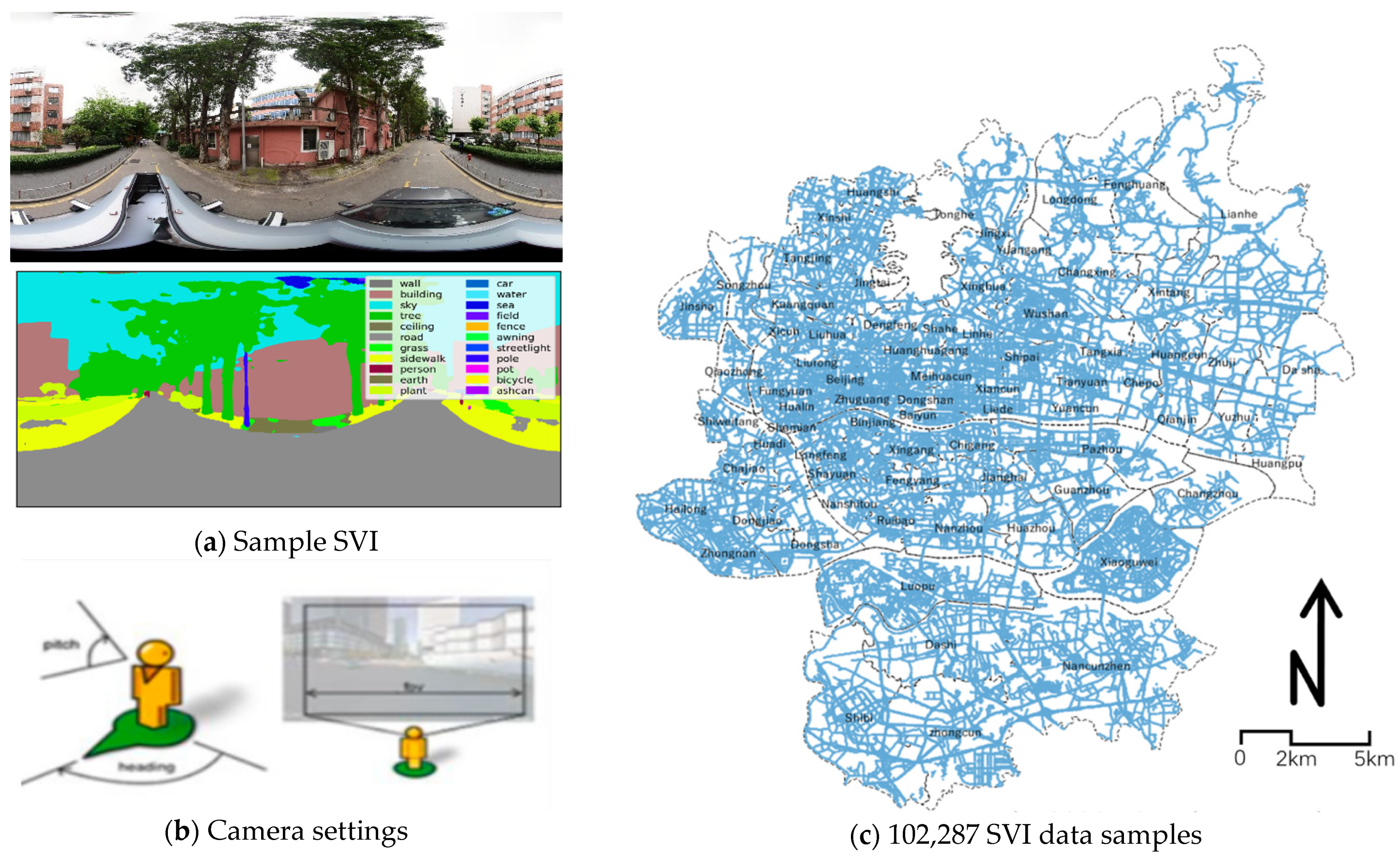
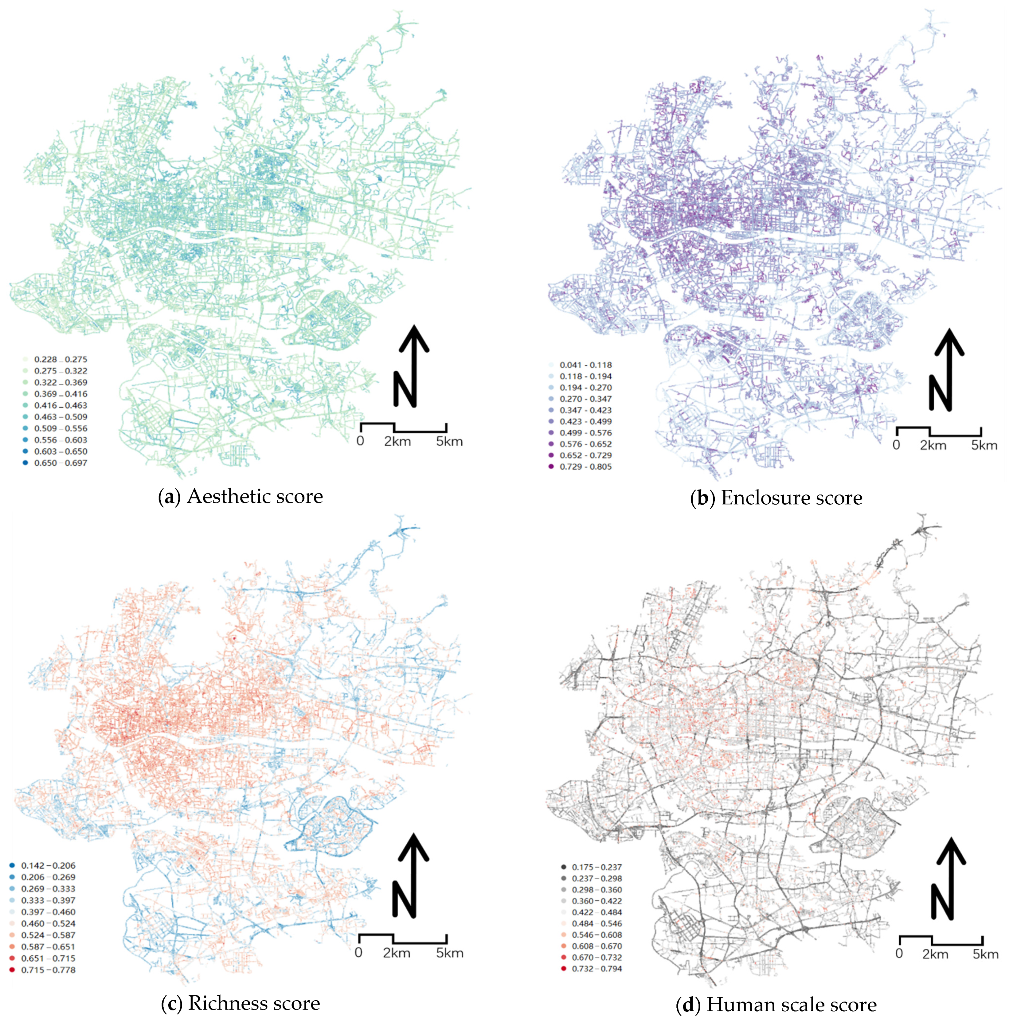
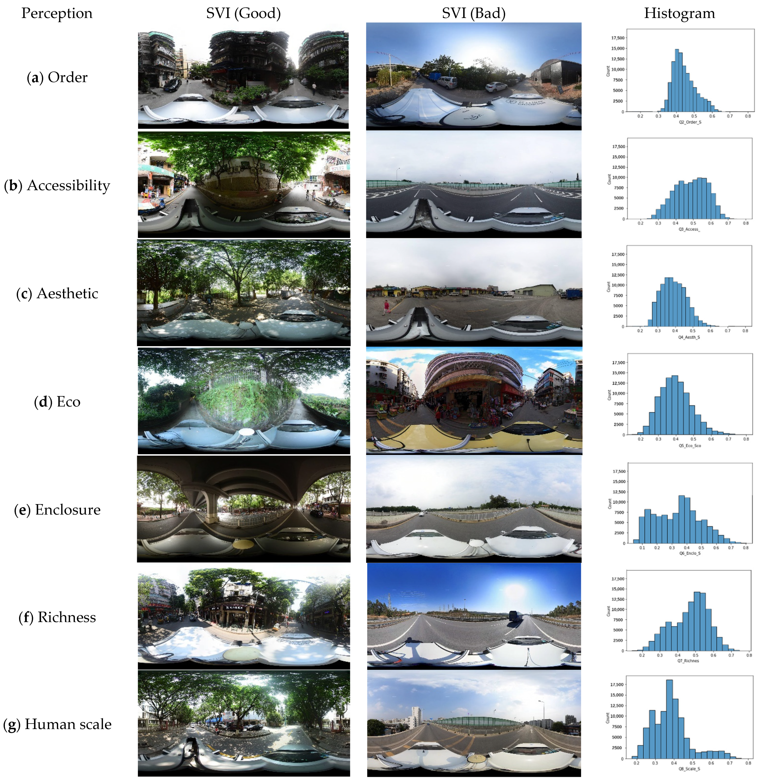
3.2.1. Streetscape Perceptual Measurements from Street-View Images
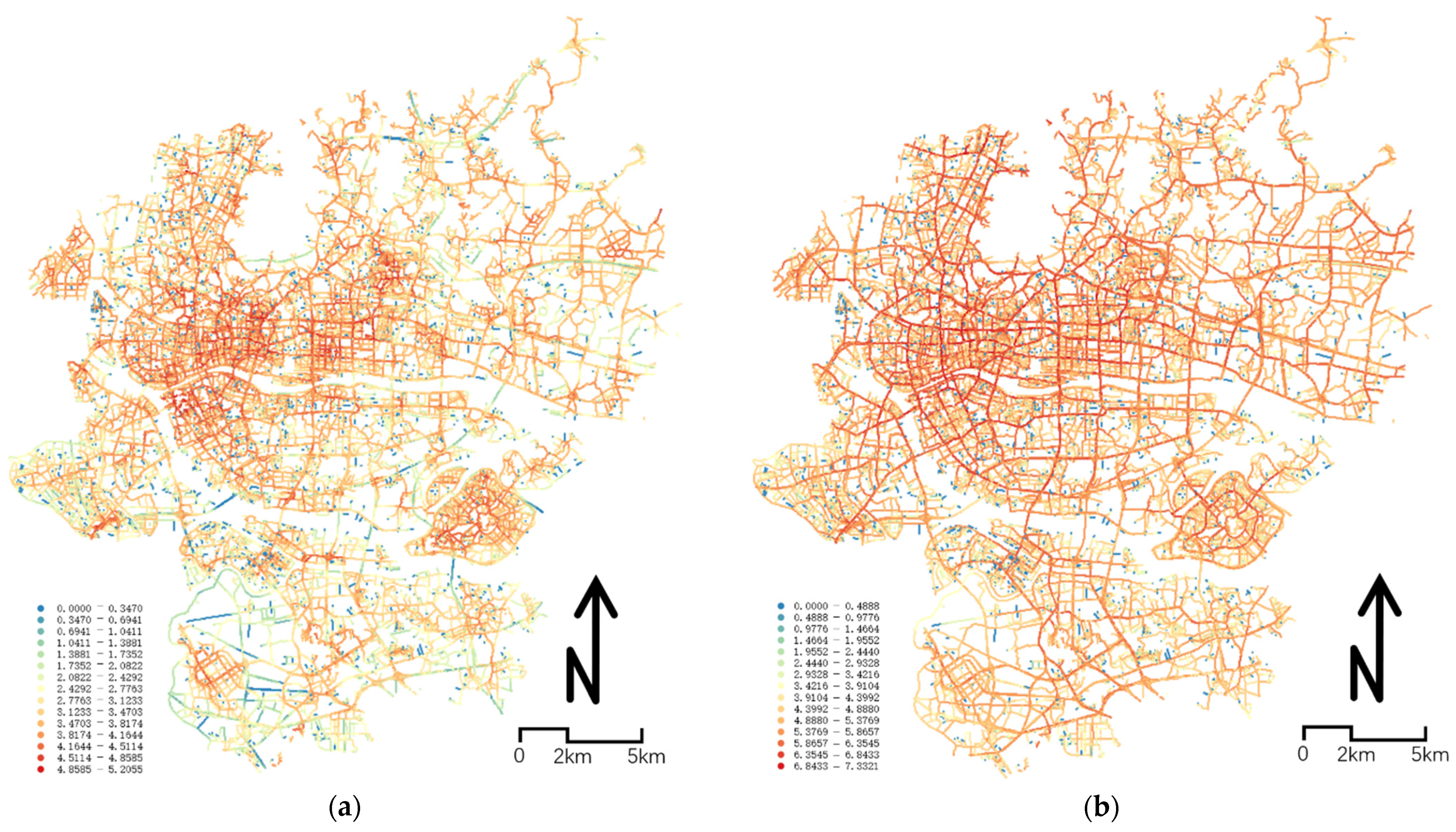
3.2.2. Through-Movement Probability Route Choice of Walking and Driving
3.2.3. Control Variables
3.2.4. Dependent Variable
3.3. Model Architecture
4. Results and Discussion
4.1. OLS Results
4.1.1. Verifying Dynamic Perception and Static Perception
4.1.2. Evaluating Walking and Driving Through-Movement Perception
4.1.3. Overall Comparison with Three Time Periods and Detailed Variables
4.2. Comparison of Related Studies
5. Conclusions
5.1. Complementary Effects between Two Modes
5.2. Implications for Urban Planning
5.3. Limitations
Author Contributions
Funding
Data Availability Statement
Conflicts of Interest
Appendix A

| OLS Regression Analyses | |||||||
|---|---|---|---|---|---|---|---|
| Selected Model | Adjusted R Square | Std Error of the Estimate | p > |t|(Sig.) | AIC | N | ||
| Baseline | All day without perception data | 0.381 | 0.003 | 0.000 *** | −16,610 | 31,526 | |
| Model 1 | All day with static perception | 0.439 | 0.005 | 0.000 *** | −19,680 | 31,526 | |
| Model 2 | All day with dynamic perception | walking | 0.442 | 0.003 | 0.000 *** | −19,860 | 31,526 |
| driving | 0.450 | 0.003 | 0.000 *** | −20,300 | 31,526 | ||
| Model 3 | All day with static and dynamic interaction model | walking | 0.453 | 0.005 | 0.000 *** | −20,500 | 31,526 |
| driving | 0.470 | 0.005 | 0.000 *** | −21,480 | 31,526 | ||
| Model 3M | Interaction model with morning vitality | walking | 0.447 | 0.005 | 0.000 *** | −19,950 | 31,526 |
| driving | 0.464 | 0.005 | 0.000 *** | −20,940 | 31,526 | ||
| Model 3N | Interaction model with noon vitality | walking | 0.425 | 0.005 | 0.000 *** | −19,280 | 31,526 |
| driving | 0.444 | 0.005 | 0.000 *** | −20,340 | 31,526 | ||
| Model 3E | Interaction model with evening vitality | walking | 0.440 | 0.005 | 0.000 *** | −22,910 | 31,526 |
| driving | 0.452 | 0.005 | 0.000 *** | −23,580 | 31,526 | ||
References
- Zeng, C.; Song, Y.; He, Q.; Shen, F. Spatially Explicit Assessment on Urban Vitality: Case Studies in Chicago and Wuhan. Sustain. Cities Soc. 2018, 40, 296–306. [Google Scholar] [CrossRef]
- Ma, X.; Ma, C.; Wu, C.; Xi, Y.; Yang, R.; Peng, N.; Zhang, C.; Ren, F. Measuring Human Perceptions of Streetscapes to Better Inform Urban Renewal: A Perspective of Scene Semantic Parsing. Cities 2021, 110, 103086. [Google Scholar] [CrossRef]
- Kang, C.; Fan, D.; Jiao, H. Validating Activity, Time, and Space Diversity as Essential Components of Urban Vitality. Environ. Plan. B Urban Anal. City Sci. 2021, 48, 1180–1197. [Google Scholar] [CrossRef]
- Kang, Y.; Zhang, F.; Gao, S.; Peng, W.; Ratti, C. Human Settlement Value Assessment from a Place Perspective: Considering Human Dynamics and Perceptions in House Price Modeling. Cities 2021, 118, 103333. [Google Scholar] [CrossRef]
- Kang, Y.; Zhang, F.; Peng, W.; Gao, S.; Rao, J.; Duarte, F.; Ratti, C. Understanding House Price Appreciation Using Multi-Source Big Geo-Data and Machine Learning. Land Use Policy 2021, 111, 104919. [Google Scholar] [CrossRef]
- Qiu, W.; Zhang, Z.; Liu, X.; Li, W.; Li, X.; Xu, X.; Huang, X. Subjective or Objective Measures of Street Environment, Which Are More Effective in Explaining Housing Prices? Landsc. Urban Plan. 2022, 221, 104358. [Google Scholar] [CrossRef]
- Buttimer, A.; Seamon, D. Body-Subject, Time-Space Routines, and Place-Ballets. In The Human Experience of Space and Place; Routledge: London, UK, 1980; ISBN 978-1-315-68419-2. [Google Scholar]
- Cresswell, T. Place: An Introduction; John Wiley & Sons: Hoboken, NJ, USA, 2014; ISBN 978-0-470-65562-7. [Google Scholar]
- Park, K.; Ewing, R.; Sabouri, S.; Larsen, J. Street Life and the Built Environment in an Auto-Oriented US Region. Cities 2019, 88, 243–251. [Google Scholar] [CrossRef]
- Li, Y.; Yabuki, N.; Fukuda, T. Exploring the Association between Street Built Environment and Street Vitality Using Deep Learning Methods. Sustain. Cities Soc. 2022, 79, 103656. [Google Scholar] [CrossRef]
- Mehta, V. Lively Streets: Determining Environmental Characteristics to Support Social Behavior. J. Plan. Educ. Res. 2007, 27, 165–187. [Google Scholar] [CrossRef]
- Lynch, K. Good City Form; MIT Press: Cambridge, MA, USA, 1984; ISBN 978-0-262-62046-8. [Google Scholar]
- Maas, P.R. Towards a Theory of Urban Vitality. Master’s Thesis, University of British Columbia, Vancouver, BC, Canada, 1984. [Google Scholar] [CrossRef]
- Shen, Y.; Karimi, K. The Economic Value of Streets: Mix-Scale Spatio-Functional Interaction and Housing Price Patterns. Appl. Geogr. 2017, 79, 187–202. [Google Scholar] [CrossRef] [Green Version]
- Sevtsuk, A. Street Commerce: Creating Vibrant Urban Sidewalks; University of Pennsylvania Press: Philadelphia, PA, USA, 2020; ISBN 978-0-8122-9708-9. [Google Scholar]
- Sevtsuk, A.; Basu, R.; Chancey, B. We Shape Our Buildings, but Do They Then Shape Us? A Longitudinal Analysis of Pedestrian Flows and Development Activity in Melbourne. PLoS ONE 2021, 16, e0257534. [Google Scholar] [CrossRef] [PubMed]
- Sevtsuk, A.; Basu, R.; Li, X.; Kalvo, R. A Big Data Approach to Understanding Pedestrian Route Choice Preferences: Evidence from San Francisco. Travel Behav. Soc. 2021, 25, 41–51. [Google Scholar] [CrossRef]
- Qiu, W.; Li, W.; Liu, X.; Huang, X. Subjectively Measured Streetscape Perceptions to Inform Urban Design Strategies for Shanghai. ISPRS Int. J. Geo-Inf. 2021, 10, 493. [Google Scholar] [CrossRef]
- Xu, X.; Qiu, W.; Li, W.; Liu, X.; Zhang, Z.; Li, X.; Luo, D. Associations between Street-View Perceptions and Housing Prices: Subjective vs. Objective Measures Using Computer Vision and Machine Learning Techniques. Remote Sens. 2022, 14, 891. [Google Scholar] [CrossRef]
- Shen, Y.; Karimi, K. Urban Evolution as a Spatio-Functional Interaction Process: The Case of Central Shanghai. J. Urban Des. 2018, 23, 42–70. [Google Scholar] [CrossRef]
- Wyly, E. The New Quantitative Revolution. Dialogues Hum. Geogr. 2014, 4, 26–38. [Google Scholar] [CrossRef]
- Dubey, A.; Naik, N.; Parikh, D.; Raskar, R.; Hidalgo, C.A. Deep Learning the City: Quantifying Urban Perception at a Global Scale. arXiv 1608. [Google Scholar] [CrossRef]
- Salesses, P.; Schechtner, K.; Hidalgo, C.A. The Collaborative Image of The City: Mapping the Inequality of Urban Perception. PLoS ONE 2013, 8, e68400. [Google Scholar] [CrossRef] [Green Version]
- Naik, N.; Philipoom, J.; Raskar, R.; Hidalgo, C. Streetscore—Predicting the Perceived Safety of One Million Streetscapes. In Proceedings of the 2014 IEEE Conference on Computer Vision and Pattern Recognition Workshops (CVPRW), Columbus, OH, USA, 23–28 June 2014; pp. 793–799. [Google Scholar] [CrossRef]
- Salazar Miranda, A.; Fan, Z.; Duarte, F.; Ratti, C. Desirable Streets: Using Deviations in Pedestrian Trajectories to Measure the Value of the Built Environment. Comput. Environ. Urban Syst. 2021, 86, 101563. [Google Scholar] [CrossRef]
- Morello, E.; Ratti, C. A Digital Image of the City: 3D Isovists in Lynch’s Urban Analysis. Environ. Plann. B 2009, 36, 837–853. [Google Scholar] [CrossRef] [Green Version]
- Ewing, R.; Handy, S.; Brownson, R.; Clemente, O.; Winston, E. Identifying and Measuring Urban Design Qualities Related to Walkability. J. Phys. Act. Health 2006, 3, S223–S240. [Google Scholar] [CrossRef] [PubMed]
- Giuliani, M.V. Theory of Attachment and Place Attachment. In Psychological Theories for Environmental Issues; Bonnes, M., Lee, T., Bonaiuto, M., Eds.; Routledge: London, UK, 2003; pp. 137–170. ISBN 978-0-7546-1888-1. [Google Scholar]
- Lewicka, M. Place Attachment: How Far Have We Come in the Last 40 Years? J. Environ. Psychol. 2011, 31, 207–230. [Google Scholar] [CrossRef]
- Raymond, C.M.; Kyttä, M.; Stedman, R. Sense of Place, Fast and Slow: The Potential Contributions of Affordance Theory to Sense of Place. Front. Psychol. 2017, 8, 1674. [Google Scholar] [CrossRef] [PubMed] [Green Version]
- Smaldone, D.; Harris, C.; Sanyal, N. An Exploration of Place as a Process: The Case of Jackson Hole, WY. J. Environ. Psychol. 2005, 25, 397–414. [Google Scholar] [CrossRef]
- Smaldone, D.; Harris, C.; Sanyal, N. The Role of Time in Developing Place Meanings. J. Leis. Res. 2008, 40, 479–504. [Google Scholar] [CrossRef]
- Brown, G.; Raymond, C. The Relationship between Place Attachment and Landscape Values: Toward Mapping Place Attachment. Appl. Geogr. 2007, 27, 89–111. [Google Scholar] [CrossRef]
- Foote, K.E.; Azaryahu, M. Sense of Place. In International Encyclopedia of Human Geography; Elsevier: Amsterdam, The Netherlands, 2009; pp. 96–100. ISBN 978-0-08-044910-4. [Google Scholar]
- Zhang, J.; Li, Q. Research on the Complex Mechanism of Placeness, Sense of Place, and Satisfaction of Historical and Cultural Blocks in Beijing’s Old City Based on Structural Equation Model. Complexity 2021, 2021, 6673158. [Google Scholar] [CrossRef]
- Ewing, R.; Handy, S. Measuring the Unmeasurable: Urban Design Qualities Related to Walkability. J. Urban Des. 2009, 14, 65–84. [Google Scholar] [CrossRef]
- Qiu, W.; Li, W.; Liu, X.; Zhang, Z.; Li, X.; Huang, X. Subjective and Objective Measures of Streetscape Perceptions: Relationships with Property Value in Shanghai. Cities 2023, 132, 104037. [Google Scholar] [CrossRef]
- Cervero, R.; Kockelman, K. Travel Demand and the 3Ds: Density, Diversity, and Design. Transp. Res. Part D Transp. Environ. 1997, 2, 199–219. [Google Scholar] [CrossRef]
- Sevtsuk, A.; Chancey, B.; Basu, R.; Mazzarello, M. Spatial Structure of Workplace and Communication between Colleagues: A Study of E-Mail Exchange and Spatial Relatedness on the MIT Campus. Soc. Netw. 2022, 70, 295–305. [Google Scholar] [CrossRef]
- Wang, B.; Xu, T.; Gao, H.; Ta, N.; Chai, Y.; Wu, J. Can Daily Mobility Alleviate Green Inequality from Living and Working Environments? Landsc. Urban Plan. 2021, 214, 104179. [Google Scholar] [CrossRef]
- Hillier, B.; Iida, S. Network and Psychological Effects in Urban Movement. In Spatial Information Theory; Cohn, A.G., Mark, D.M., Eds.; Lecture Notes in Computer Science; Springer: Berlin/Heidelberg, Germany, 2005; Volume 3693, pp. 475–490. ISBN 978-3-540-28964-7. [Google Scholar]
- Hillier, B.; Penn, A.; Hanson, J.; Grajewski, T.; Xu, J. Natural Movement: Or, Configuration and Attraction in Urban Pedestrian Movement. Environ. Plan. B Plan. Des. 1993, 20, 29–66. [Google Scholar] [CrossRef] [Green Version]
- Shen, Y. Understanding Functional Urban Centrality: Spatio-Functional Interaction and Its Socio-Economic Impact in Central Shanghai. Ph.D. Thesis, UCL (University College London), London, UK, 2017. [Google Scholar]
- Lerman, Y.; Rofè, Y.; Omer, I. Using Space Syntax to Model Pedestrian Movement in Urban Transportation Planning: Using Space Syntax in Transportation Planning. Geogr. Anal. 2014, 46, 392–410. [Google Scholar] [CrossRef]
- Koohsari, M.J.; Oka, K.; Owen, N.; Sugiyama, T. Natural Movement: A Space Syntax Theory Linking Urban Form and Function with Walking for Transport. Health Place 2019, 58, 102072. [Google Scholar] [CrossRef]
- Sutkaitytė, M. Human Behaviour Simulation Using Space Syntax Methods. Archit. Urban Plan. 2020, 16, 84–92. [Google Scholar] [CrossRef]
- Basu, N.; Haque, M.M.; King, M.; Kamruzzaman, M.; Oviedo-Trespalacios, O. A Systematic Review of the Factors Associated with Pedestrian Route Choice. Transp. Rev. 2022, 42, 672–694. [Google Scholar] [CrossRef]
- Ye, Y.; Xie, H.; Fang, J.; Jiang, H.; Wang, D. Daily Accessed Street Greenery and Housing Price: Measuring Economic Performance of Human-Scale Streetscapes via New Urban Data. Sustainability 2019, 11, 1741. [Google Scholar] [CrossRef]
- Ye, Y.; Richards, D.; Lu, Y.; Song, X.; Zhuang, Y.; Zeng, W.; Zhong, T. Measuring Daily Accessed Street Greenery: A Human-Scale Approach for Informing Better Urban Planning Practices. Landsc. Urban Plan. 2019, 191, 103434. [Google Scholar] [CrossRef]
- Montgomery, J. Café Culture and the City: The Role of Pavement Cafés in Urban Public Social Life. J. Urban Des. 1997, 2, 83–102. [Google Scholar] [CrossRef]
- Glaeser, E.L.; Kim, H.; Luca, M. Nowcasting Gentrification: Using Yelp Data to Quantify Neighborhood Change. AEA Pap. Proc. 2018, 108, 77–82. [Google Scholar] [CrossRef] [Green Version]
- Mouratidis, K.; Poortinga, W. Built Environment, Urban Vitality and Social Cohesion: Do Vibrant Neighborhoods Foster Strong Communities? Landsc. Urban Plan. 2020, 204, 103951. [Google Scholar] [CrossRef]
- Ferreira, J.; Ferreira, C.; Bos, E. Spaces of Consumption, Connection, and Community: Exploring the Role of the Coffee Shop in Urban Lives. Geoforum 2021, 119, 21–29. [Google Scholar] [CrossRef]
- Chen, Z.; Dong, B.; Pei, Q.; Zhang, Z. The Impacts of Urban Vitality and Urban Density on Innovation: Evidence from China’s Greater Bay Area. Habitat Int. 2022, 119, 102490. [Google Scholar] [CrossRef]
- Li, Q.; Cui, C.; Liu, F.; Wu, Q.; Run, Y.; Han, Z. Multidimensional Urban Vitality on Streets: Spatial Patterns and Influence Factor Identification Using Multisource Urban Data. IJGI 2021, 11, 2. [Google Scholar] [CrossRef]
- Ewing, R. Is Los Angeles-Style Sprawl Desirable? J. Am. Plan. Assoc. 1997, 63, 107–126. [Google Scholar] [CrossRef]
- Long, Y.; Huang, C. Does Block Size Matter? The Impact of Urban Design on Economic Vitality for Chinese Cities. Environment and Planning B: Urban Analytics and City Science 2017, 46, 406–422. [Google Scholar] [CrossRef] [Green Version]
- Duranton, G.; Puga, D. The Economics of Urban Density. J. Econ. Perspect. 2020, 34, 3–26. [Google Scholar] [CrossRef]
- Zhang, Z.; Zhang, Y.; He, T.; Xiao, R. Urban Vitality and Its Influencing Factors: Comparative Analysis Based on Taxi Trajectory Data. IEEE J. Sel. Top. Appl. Earth Obs. Remote Sens. 2022, 15, 5102–5114. [Google Scholar] [CrossRef]
- Jacobs, J. The Death and Life of Great American Cities; Knopf Doubleday Publishing Group: New York, NY, USA, 1961; ISBN 978-0-394-42159-9. [Google Scholar]
- Ratti, C. Space Syntax: Some Inconsistencies. Environ. Plann. B Plann. Des. 2004, 31, 487–499. [Google Scholar] [CrossRef]
- Hillier, B. Studying Cities to Learn about Minds: Some Possible Implications of Space Syntax for Spatial Cognition. Environ. Plann. B Plann. Des 2012, 39, 12–32. [Google Scholar] [CrossRef]
- Hillier, B. Space Is the Machine: A Configurational Theory of Architecture; Space Syntax: London, UK, 2015; ISBN 978-1-5116-9776-7. [Google Scholar]
- Barnard, A. The Legacy of the Situationist International: The Production of Situations of Creative Resistance. Cap. Cl. 2004, 28, 103–124. [Google Scholar] [CrossRef]
- Gunn, G. 4—In Revolutionary Guangzhou; Cambridge University Press: Cambridge, UK, 2021; pp. 98–125. ISBN 978-1-108-97380-9. [Google Scholar]
- Ipsen, D.; Li, Y.; Weichler, H. (Eds.) The Genesis of Urban Landscape: The Pearl River Delta in South China; Work Report/University of Kassel, Faculty of Architecture, Urban Planning, Landscape Planning; University of Kassel: Kassel, Germany, 2005; ISBN 978-3-89117-153-0. [Google Scholar]
- Guangzhou Aims to Become a Global City—Cities in Motion. Available online: https://blog.iese.edu/cities-challenges-and-management/2018/06/04/guangzhou-aims-to-become-a-global-city/ (accessed on 14 October 2022).
- Tian, H.; Han, Z.; Xu, W.; Liu, X.; Qiu, W.; Li, W. Evolution of Historical Urban Landscape with Computer Vision and Machine Learning: A Case Study of Berlin. J. Digit. Landsc. Archit. 2021, 16, 436–445. [Google Scholar] [CrossRef]
- Shen, Y.; Karimi, K. Urban Function Connectivity: Characterisation of Functional Urban Streets with Social Media Check-in Data. Cities 2016, 55, 9–21. [Google Scholar] [CrossRef] [Green Version]
- Turner, A. From Axial to Road-Centre Lines: A New Representation for Space Syntax and a New Model of Route Choice for Transport Network Analysis. Environ. Plann. B Plann. Des. 2007, 34, 539–555. [Google Scholar] [CrossRef] [Green Version]
- Omer, I.; Kaplan, N.; Jiang, B. Why angular centralities are more suitable for space syntax modeling? In Proceedings of the 11th International Space Syntax Symposium, Lisbon, Portugal, 3–7 July 2017. [Google Scholar]
- Walford, G.; Tucker, E.; Viswanathan, M. The SAGE Handbook of Measurement; SAGE: Thousand Oaks, CA, USA, 2010; ISBN 978-1-4462-0688-1. [Google Scholar]
- Hillier, B. Cities as Movement Economies. Urban Des. Int. 1996, 1, 41–60. [Google Scholar] [CrossRef]
- Burke, M.; Brown, L. Distances People Walk for Transport. Road Transp. Res. 2007, 16, 16–29. [Google Scholar]
- Varoudis, T. DepthmapX MultiPlatform Spatial Network Analysis Software, Version 0.50. 2012. Available online: https://varoudis.github.io/depthmapX/ (accessed on 13 November 2022).
- Jiang, B.; Jia, T. Zipf’s Law for All the Natural Cities in the United States: A Geospatial Perspective. Int. J. Geogr. Inf. Sci. 2011, 25, 1269–1281. [Google Scholar] [CrossRef]
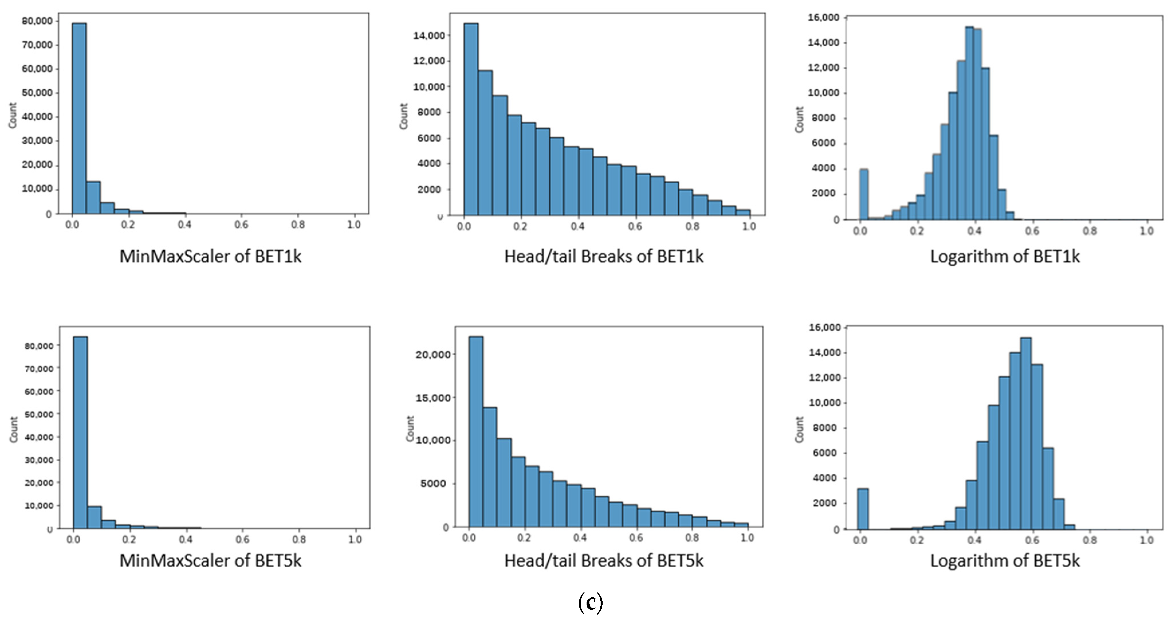
- Jiang, B. Head/Tail Breaks: A New Classification Scheme for Data with a Heavy-Tailed Distribution. Prof. Geogr. 2013, 65, 482–494. [Google Scholar] [CrossRef]
- Su, N.; Li, W.; Qiu, W. Measuring the Associations between Eye-Level Urban Design Quality and on-Street Crime Density around New York Subway Entrances. Habitat Int. 2023, 131, 102728. [Google Scholar] [CrossRef]
- Chuvieco, E. Measuring Changes in Landscape Pattern from Satellite Images: Short-Term Effects of Fire on Spatial Diversity. Int. J. Remote Sens. 1999, 20, 2331–2346. [Google Scholar] [CrossRef]
- Zhang, H. Extracting Active Population Data Based on Baidu Heat Maps for Transportation Planning Applications. Urban Transp. China 2021, 19, 103–111. [Google Scholar]
- Wu, Z.; Ye, Z. Research on Urban Spatial Structure Based on Baidu Heat Map: A Case Study on the Central City of Shanghai. City Plan. Rev. 2016, 0, 33–40. [Google Scholar] [CrossRef]
- Niu, X.; Wu, W.; Li, M. Influence of Built Environment on Street Vitality and Its Spatiotemporal Characteristics Based on LBS Positioning Data. UPI 2019, 34, 28–37. [Google Scholar] [CrossRef]
- Lin, X.; Wang, G.; Hu, Y. Characteristics of the Jobs-Housing Balance in Central Guangzhou Based on Open Big Data. Trop. Geogr. 2020, 40, 254–265. [Google Scholar] [CrossRef]
- Wang, H.; Kifer, D.; Graif, C.; Li, Z. Crime Rate Inference with Big Data. In Proceedings of the Proceedings of the 22nd ACM SIGKDD International Conference on Knowledge Discovery and Data Mining, San Francisco, CA, USA, 13–17 August 2016; pp. 635–644. [Google Scholar]
- Kutner, M.H.; Nachtsheim, C.; Neter, J. Applied Linear Regression Models; McGraw-Hill: New York, NY, USA, 2004; ISBN 978-0-07-238691-2. [Google Scholar]
- Urban, D.; Mayerl, J. Angewandte Regressionsanalyse: Theorie, Technik und Praxis; Springer: Berlin/Heidelberg, Germany, 2018; ISBN 978-3-658-01915-0. [Google Scholar]
- Nourian, P.; Rezvani, S.; Sariyildiz, S.; van der Hoeven, F. Spectral Modelling for Spatial Network Analysis. In Proceedings of the Symposium on Simulation for Architecture and Urban Design (simAUD 2016), London, UK, 16–18 May 2016. [Google Scholar]
- Nourian, P.; Rezvani, S.; Valeckaite, K.; Sariyildiz, S. Modelling Walking and Cycling Accessibility and Mobility: The Effect of Network Configuration and Occupancy on Spatial Dynamics of Active Mobility. Smart Sustain. Built Environ. 2018, 7, 101–116. [Google Scholar] [CrossRef]


| Variable | Syncopate | Description | Count | Mean | Std.Dev. | Min | Max | Data Source and Access Time |
|---|---|---|---|---|---|---|---|---|
| Spatiotemporal Vitality attributes | ||||||||
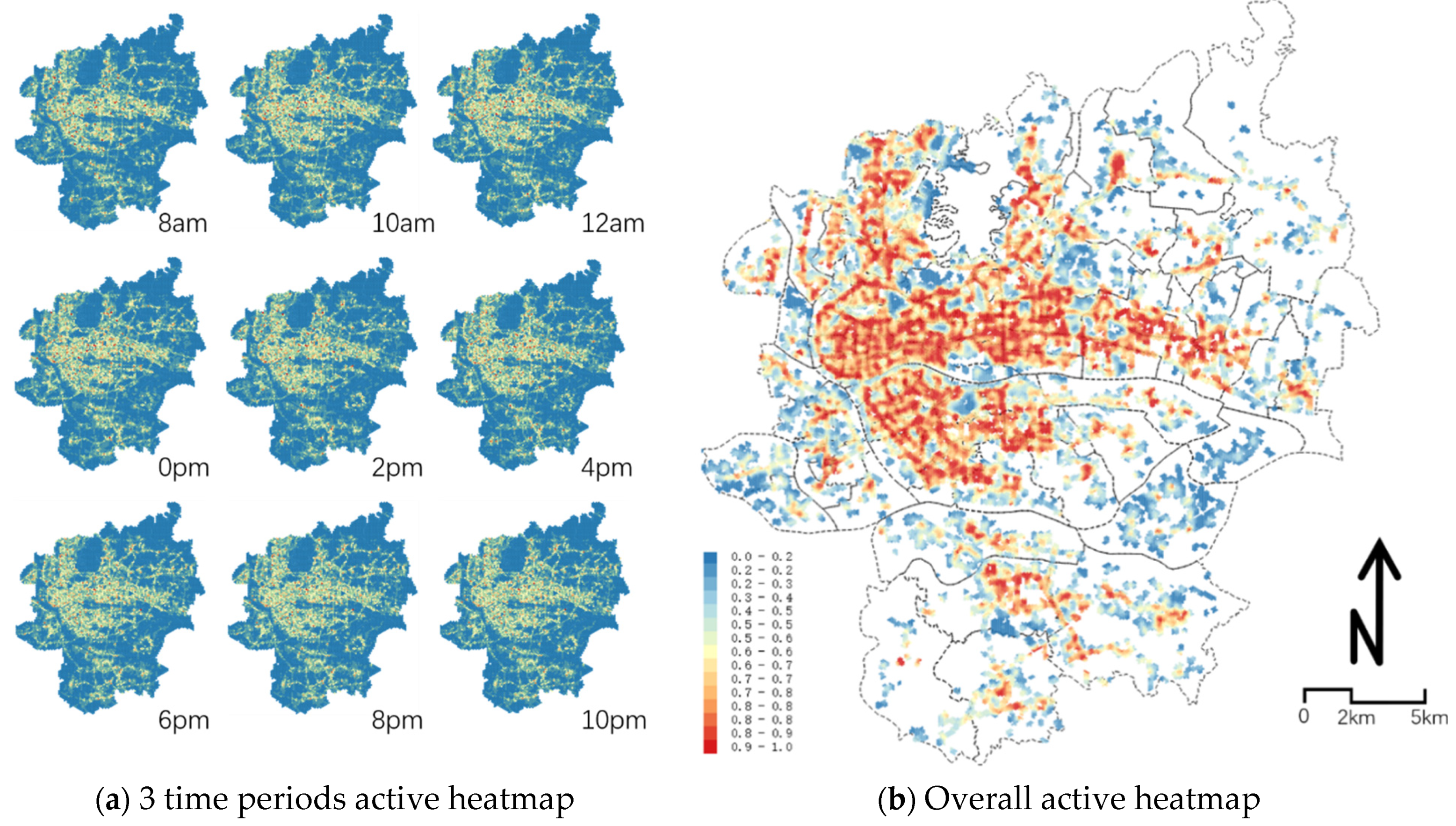
| Vitality overal | AllHeat | The overall active population in all time periods | 101,035 | 720.978 | 556.843 | 0 | 3319.38 | Scraping from Baidu API and calculated in QGIS (2022) |
| Vitality morning | Mor_Heat | The morning active population | 220.042 | 158.938 | 0 | 1194.273 | ||
| Vitality noon | Noo_Heat | The noon active population | 275.355 | 199.553 | 0 | 1351.23 | ||
| Vitality evening | Eve_Heat | The evening active population | 225.582 | 180.555 | 0 | 917.633 | ||
| Functional-based attributes | ||||||||
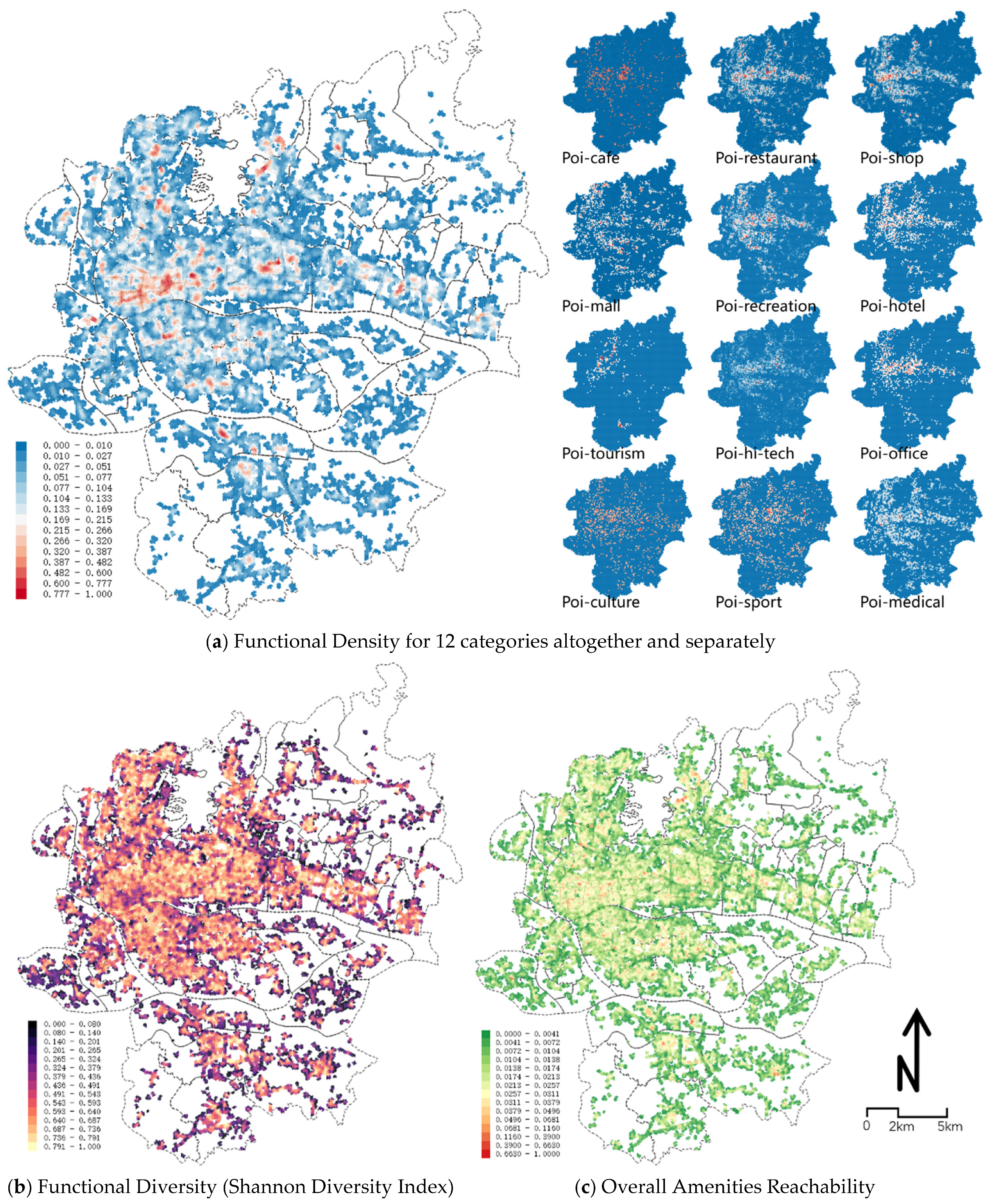
| Shannon_Wiener_Diversity | FDI | POI Functional Diversity | 39,375 | 1.12 | 1.224 | 0.017 | 2.242 | Scraping from Amap API and calculated in QGIS (2021) |
| Functional Density | FDE | POI Functional Density | 26.82 | 12 | 1 | 414 | ||
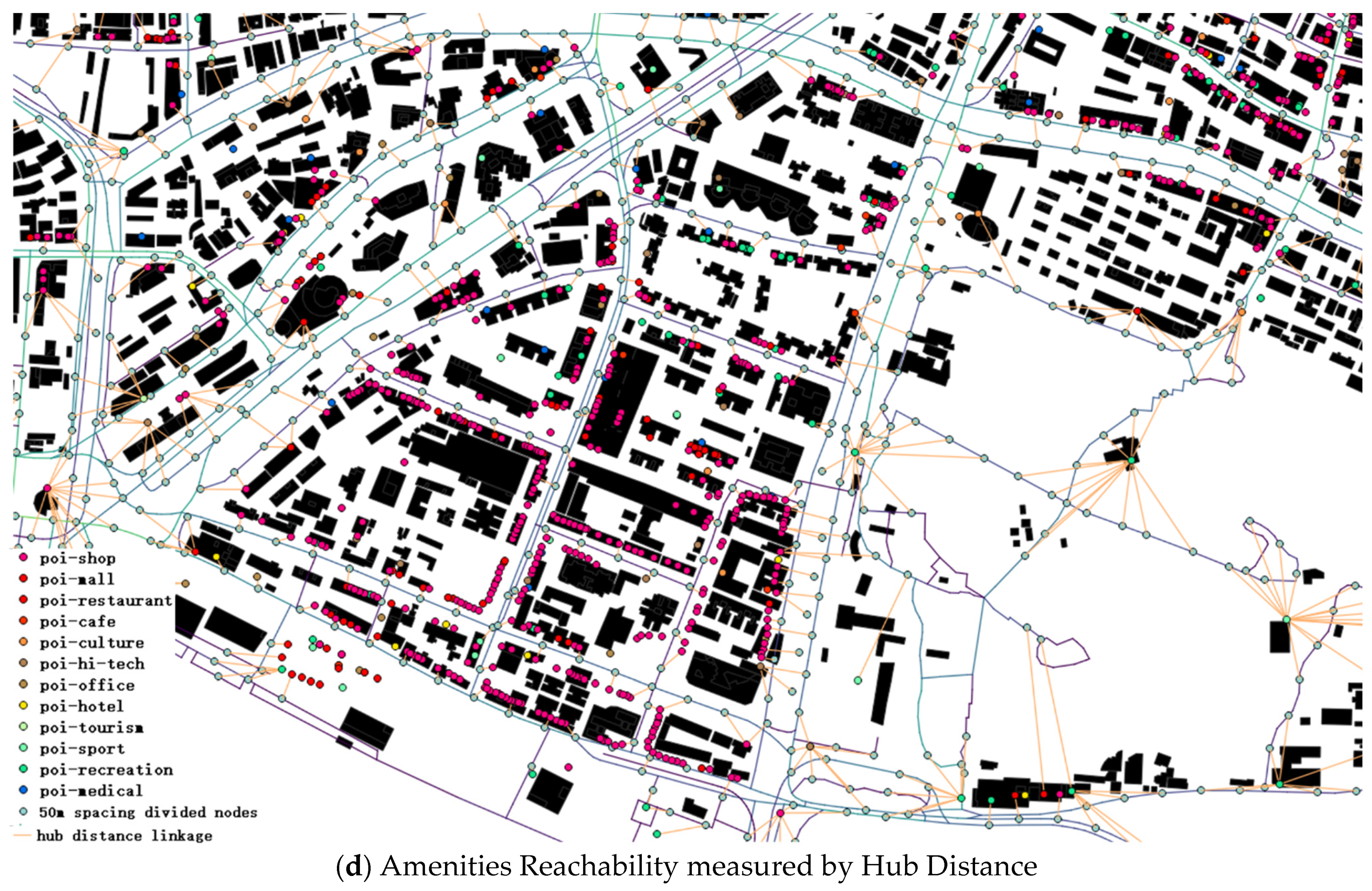
| Amenities reachability | ACR | Reachability from each segment to POIs | 0.031 | 0.027 | 0.004 | 1.923 | ||
| Static Streetscape attributes | ||||||||
| Aesth_Score | AESHT | Perceived Aesthetic | 102,287 | 0.394 | 0.39 | 0.228 | 0.697 | Predicted by ML models with view indices extracted from SVIs (2022) |
| Enclo_Score | ENCLO | Perceived Enclosure | 0.341 | 0.353 | 0.041 | 0.805 | ||
| Richness_Score | RICHN | Perceived Richness | 0.469 | 0.486 | 0.142 | 0.778 | ||
| Scale_Score | SCALE | Perceived Human scale | 0.383 | 0.376 | 0.175 | 0.794 | ||
| Through-movement probability attributes | ||||||||
| Choice/Betweenness 1 km | BET1k | Logarithm of Betweenness/Choice 1 km | 101,035 | 3.211 | 3.415 | 0 | 5.205 | Guangzhou Road Network Shapefile (2019) and calculated in Depthmap |
| Choice/Betweenness 5 km | BET5k | Logarithm of Betweenness/Choice 5 km | 5.063 | 5.308 | 0 | 7.332 | ||
| Attributes interaction in dynamic models | ||||||||
| Aesth_Score * choice1k | AESTH_BET1k | Perceived Aesthetic through walking | 39,375 | Predicted by ML models with view indices extracted from SVIs and multiply by Choice1km and Choice5km respectively, and normalized in the same sampled data points | ||||
| Enclo_Score * choice1k | ENCLO_BET1k | Perceived Enclosure through walking | ||||||
| Richness_Score * choice1k | RICHN_BET1k | Perceived Richness through walking | ||||||
| Scale_Score * choice1k | SCALE_BET1k | Perceived Human scale through walking | ||||||
| Aesth_Score * choice5k | AESHT_BET5k | Perceived Aesthetic through driving | ||||||
| Enclo_Score * choice5k | ENCLO_BET5k | Perceived Enclosure through driving | ||||||
| Richness_Score * choice5k | RICHN_BET5k | Perceived Richness through driving | ||||||
| Scale_Score * choice5k | SCALE_BET5k | Perceived Human scale through driving | ||||||
| Selected Model | Adjusted R Square | Std Error of the Estimate | AIC | N | ||
|---|---|---|---|---|---|---|
| Baseline | All day without perception data | 0.381 *** | 0.003 | −16,610 | 31,526 | |
| Model 1 | All day with static perception | 0.439 *** | 0.005 | −19,680 | 31,526 | |
| Model 2 | All day with dynamic perception | walking | 0.442 *** | 0.003 | −19,860 | 31,526 |
| driving | 0.450 *** | 0.003 | −20,300 | 31,526 | ||
| Model 3 | All day with static and dynamic interaction model | walking | 0.453 *** | 0.005 | −20,500 | 31,526 |
| driving | 0.470 *** | 0.005 | −21,480 | 31,526 | ||
| Variable | VIF | Model3-Walking | Model3-Driving | ||
|---|---|---|---|---|---|
| Intercept | 27.62 | Coefficient | Std Err | Coefficient | Std Err |
| FDI | 1.64 | 0.35 *** | 0.006 | 0.33 *** | 0.006 |
| FDE | 1.66 | 0.64 *** | 0.014 | 0.60 *** | 0.014 |
| ACR | 1.60 | −0.7 *** | 0.092 | −0.60 *** | 0.091 |
| AESTH | 2.52 | −0.31 *** | 0.02 | −0.38 *** | 0.018 |
| ENCLO | 4.44 | 0.13 *** | 0.024 | 0.30 *** | 0.021 |
| RICHN | 2.16 | 0.28 *** | 0.017 | 0.27 *** | 0.015 |
| SCALE | 4.89 | −0.03 | 0.032 | −0.05 * | 0.027 |
| BET1k | 1.90 | ||||
| BET5k | 1.96 | ||||
| AESTH_BET1k | −0.27 *** | 0.057 | |||
| ENCLO_BET1k | 0.03 | 0.066 | |||
| RICHN_BET1k | 0.53 *** | 0.037 | |||
| SCALE_BET1k | −0.16 ** | 0.084 | |||
| AESTH_BET5k | −0.07 * | 0.056 | |||
| ENCLO_BET5k | −0.26 *** | 0.065 | |||
| RICHN_BET5k | 0.67 *** | 0.036 | |||
| SCALE_BET5k | −0.06 | 0.078 | |||
| Adjusted R square | 0.453 | 0.47 | |||
| AIC | −20,500 | −21,480 | |||
| BIC | −20,400 | −21,380 | |||
Disclaimer/Publisher’s Note: The statements, opinions and data contained in all publications are solely those of the individual author(s) and contributor(s) and not of MDPI and/or the editor(s). MDPI and/or the editor(s) disclaim responsibility for any injury to people or property resulting from any ideas, methods, instructions or products referred to in the content. |
© 2023 by the authors. Licensee MDPI, Basel, Switzerland. This article is an open access article distributed under the terms and conditions of the Creative Commons Attribution (CC BY) license (https://creativecommons.org/licenses/by/4.0/).
Share and Cite
Wang, Y.; Qiu, W.; Jiang, Q.; Li, W.; Ji, T.; Dong, L. Drivers or Pedestrians, Whose Dynamic Perceptions Are More Effective to Explain Street Vitality? A Case Study in Guangzhou. Remote Sens. 2023, 15, 568. https://doi.org/10.3390/rs15030568
Wang Y, Qiu W, Jiang Q, Li W, Ji T, Dong L. Drivers or Pedestrians, Whose Dynamic Perceptions Are More Effective to Explain Street Vitality? A Case Study in Guangzhou. Remote Sensing. 2023; 15(3):568. https://doi.org/10.3390/rs15030568
Chicago/Turabian StyleWang, Yuankai, Waishan Qiu, Qingrui Jiang, Wenjing Li, Tong Ji, and Lin Dong. 2023. "Drivers or Pedestrians, Whose Dynamic Perceptions Are More Effective to Explain Street Vitality? A Case Study in Guangzhou" Remote Sensing 15, no. 3: 568. https://doi.org/10.3390/rs15030568