Feature Selection for Airbone LiDAR Point Cloud Classification

Abstract

The classification of airborne LiDAR data is a prerequisite for many spatial data elaborations and analysis. In the domain of power supply networks, it is of utmost importance to be able to discern at least five classes for further processing—ground, buildings, vegetation, poles, and catenaries. This process is mainly performed manually by domain experts with the use of advanced point cloud manipulation software. The goal of this paper is to find a set of features which would divide space well enough to achieve accurate automatic classification on all relevant classes within the domain, thus reducing manual labor. To tackle this problem, we propose a single multi-class approach to classify all four basic classes (excluding ground) in a power supply domain with single pass-through, using one network. The proposed solution implements random forests and gradient boosting to create a feature-based per-point classifier which achieved an accuracy and F1 score of over 99% on all tested cases, with the maximum of 99.7% for accuracy and 99.5% for F1 score. Moreover, we achieved a maximum of 81.7% F1 score for the most sparse class. The results show that the proposed set of features for the LiDAR data cloud is effective in power supply line classification.

1. Introduction

The analysis of data collected with the use of Airborne Light Detection And Ranging (LiDAR) has been of interest to many researchers for many years now, and has become an industry standard for many applications. The most important challenge in this domain is to develop automatic element extraction and classification algorithms for a given cloud of points which describes different classes, such as ground, vegetation, or buildings. The main focus in this research field lies in building extraction and classification. The ability to identify buildings is widely used in city planning, or preparing 3D models of buildings or even whole cities. Moreover, when dealing with power supplies, it is necessary to identify human settlements since they are immovable objects, and various standards have to be met in the process of planning the route of high voltage cables regarding the distance from buildings. Concerning the building extraction problem, much effort is made to localize the roof edges, since many standard methods mistakenly identify roofs as a ground. Moreover, the points belonging to the edge of the roof make detection difficult because refractions change the angle of laser reflection, which may result in the incorrect recording of point features.

In addition to detecting buildings, much research within LiDAR data processing has been performed on the separation of power lines and electricity poles. This is widely used in the energy industry, where determining the exact course of the power grid allows for faster and more accurate maintenance.

The detection of individual elements from the point cloud in such studies allows for the generation of analyses to maintain an uninterrupted supply of electricity. The evaluation of vegetation is performed most often, with particular emphasis on the detection of threatening trees and the dangerous proximity of powerlines to buildings and other objects. Moreover, great importance within such studies is placed on maintaining energy standards in the field of electromagnetic field interference on people, the detection of cable deflections, and the resulting changes in distances to objects, depending on the current flow and weather conditions. Very dense laser coatings are necessary to achieve satisfactory research results, which either causes the use of very expensive equipment or determines very low air raids (120–200 m above the ground), which excludes aircraft raids. Therefore, there are additional difficulties in processing the point cloud. In the case of buildings, apart from detecting roofs and their edges, additional hassle comes from the need to detect the walls and elements of the building equipment.

The main contribution of this paper covers the preparation of novel solutions supporting the work at Visimind Ltd, where the main research effort is focused on the analysis of power supply and distribution companies, which requires a correct classification of vegetation, catenaries, and electrical poles, besides buildings and the ground. Most state of the art studies focus on one or two class classifiers, with limited work regarding powerlines. Most work on power lines were performed to discern power cables and sometimes pylons as well, but they usually require a highly complicated mix of computer vision and machine learning techniques. This contribution shows that it is possible to both detect classes that are well described in different works such as buildings or vegetation, and power supply specific classes, as well as during one pass-through with one network.

Currently, Visimind Ltd. like many others, uses basic classification solutions that generate a lot of errors. All of the errors made during classification have to be corrected manually later on, which is both time and resource consuming. For this reason, this paper focuses on creating effective, highly accurate classifiers that will be able to classify the basic set of classes used in power distribution network analysis—vegetation, buildings, catenaries (powerline cables), and poles.

The ground, although very important, is beyond the scope of this paper. Ground detection is an industry standard in many domains that use airborne LiDARs, and companies around the world had already established a workflow to perform this process effectively. As a result, ground classification is not as time-consuming as other parts of classification and yields stronger automatic results. This topic has been and still is a matter of different research on its own, but we believe it is a solved issue for business use. Most companies use widely adopted point cloud manipulation software such as TerraSolid that is able to perform accurate automatic ground detection and does not require much manual correction. This process may be inaccurate in difficult terrain (such as high mountain areas and very rocky terrain), where it requires more extensive manual corrections; therefore, in some projects, this stage may be more labor expensive than in others. However, while every company has different quality standards for preliminary ground classification, it is worth noting that many analyses are based on digital terrain models (DTMs), which implies that companies are going to invest time in perfecting the ground. Hence, we used in our research ground detected using TerraSolid, and manually corrected, as would have been performed during normal data elaboration; therefore, it does not affect the quality of the training data.

The algorithm proposed in this paper uses ground to determine height-based features that are based on the height relative to the ground, and so it requires a digital terrain model from the ground points. There is no case for where our classifier will try to reclassify ground into any different class, nor are the ground points themselves used in feature properties extraction. We do not generate any additional errors in that regard. Only the resulting DTM is used for relative height acquisition.

To achieve significant advances in the workflow of the company, the authors proposed novel methods based on classical random forests and the XGBoost classifier. During our research, we were able to discern certain features and to apply random forests to yield on par or better than state-of-the-art results. The innovation of our method comes from a unique combination of known features, and some that we propose to introduce for this problem. We are able to show that by using this set of features, in combination with random forests, one can have a single pass-through classifier for all classes needed for elaboration in a problem domain. We have demonstrated that it is possible to have a multi-class per-point classifier with four classes of different occurrences that can still achieve over 99% accuracy on all of them while maintaining F1 scores over 80%.

During the feature engineering phase, three main groups of characteristics have been defined, based on the height above the ground, and based on reflection and geometry. In addition, each feature has been developed and calculated using a different neighborhood selection method. Finally, a floating-point value was specified for each of the features after the transformations.

During the experimental session, it turned out that the classification with the use of XGBoost achieves much better results than in the case of random forests, where both of the calculated parameters: the accuracy and the F1 measure, achieved values of around 94–96%, depending on the input parameters for the XGBoost method.

What is very important in the light of the obtained results is that the level of precision and recall does not decrease in the case of the classification of points determining the poles of high voltage lines, whereas in the first stages of the research, the biggest problem was the extremely low efficiency of pole detection.

In addition, in the experimental phase, our solutions based on the XGBoost were compared with similar research related to feature extraction, and the solution described in this paper achieves the best results. It is especially visible in experiments on the detection of poles, where our algorithm achieves the F1 measure by greater than 20%, compared to the other state of the art methods.

The rest of the paper is organized as follows. In the next section, we review the existing solutions for LiDAR data classification. The main contribution of this paper is introduced in Section 3, where the proposed feature selection methodology and description of classification algorithms is provided. Next, Section 4 evaluates the proposed approach based on experimental results. We conclude and point future directions in Section 5.

2. Related Work

Research aimed at identifying elements of various classes from the point cloud provided with the LiDAR system is mainly focused on detecting buildings. Many groups of scientists confront the aforementioned problem and propose various methods to separate edifices from surroundings. One of the approaches used in such investigations is roof edge detection. The authors in [1] followed this direction, and proposed a solution based on semi-suppressed fuzzy C-means and restricted region growing. The use of the aforementioned algorithms not only made it possible to deal with simple roofs, but also elliptical ones. Further research, which takes advantage of restriction region growing in post-processing, is proposed in [2], which developed methods for discriminating building points from vegetation with the use of minimum cut. Moreover, it should be noted that the use of neural networks in detecting buildings has become more popular in recent years. Examples of such applications are [3], where the author implemented Convolutional Neural Networks for building detection, and [4], who proposed methods based on Multilayered Feedforward Neural Networks for tree and building classification. Moreover, in [5], Deep Neural Networks were implemented in the building detection process. The authors point out that owing to the use of such a solution, there is no need for the careful selection of the characteristics of individual points, since the introduction of Deep Neural Networks for LiDAR data allows for the achievement of similar results to other detection building techniques. A slightly different approach in the building detection domain was shown in [6], which focused more on detecting information about building heights than on commonly studied horizontal features. Local Moran’s I spatial statistics and Kernel Density Estimation for LiDAR point cloud datasets methods were used in order to explore vertical urban patterns.

To investigate the previously described solutions in the field of urban element detection, refer to the summary of the state of the art methods proposed in [7,8]. All of the described solutions process data with unsupervised algorithms for building detection.

The second widely used group of algorithms in point cloud processing concerns supervised learning algorithms, the purpose of which is to classify the labeled data.

In this case, the conducted research uses various classification algorithms and takes into account various datasets for creating models. Among the methods used, it is worth paying attention to the use of Deep Neural Networks. The authors in [9] implemented two coupled Convolutional Neural Networks (CNNs) in the classification process, while in [10], a deep encoder–decoder network architecture was selected. Both approaches used two state of the art datasets for evaluation. The Houston dataset includes a LiDAR image with one band the size of 349 × 1905 pixels, whereas Trento consists of an image with a spatial size of 166 × 600 pixels. In the first dataset, LiDAR points were divided into 15 classes, while in the second one, into 5 classes. The authors in [9] reported an accuracy on the level of 96% for the Houston dataset, and 99% for Trento. In contrast, [10] found a tier of 88% and 94%, respectively.

Another algorithm often implemented in point cloud classification is random forests. The main goal of [11,12] was to select the data features that most significantly determine class membership. For this reason, the authors chose the random forests method, since it can measure the individual variable importance.

The summary of LiDAR point classification techniques should also include [13], which is the most similar to the research presented in this work. It first uses correlation analysis to select the features of the point cloud for experiments. It then performs preprocessing to extract the observations of terrain, and finally uses JointBoost to classify the remaining points into the following classes: buildings, vegetation, power lines, and poles. The authors reported an overall accuracy of around 95% on the dedicated test dataset. However, this high accuracy may be due to a very unbalanced dataset.

Another important direction related to the research described in this paper is the detection and classification of power lines and pylons.

Ref. [14] is a proposal of a comprehensive method of powerline classification using the appropriate pre-selection of points, reducing the scene and finally using the SVM. The enormous overhead of data preprocessing in a targeted manner significantly limits the possibility of using the proposed solution in more general cases. A similar approach is presented in [15]. The authors divide the entire process into three tasks for the purpose of classifying pylons and power lines. The first shows the route of high-voltage lines, the second classifies buildings, and the last one identifies poles. As in the previous case, it significantly limits the classification of various objects among LiDAR points. Further studies focusing on the extraction of power lines and pylons were included in [16]. The proposed solution achieves high values of correctness and completeness parameters, but it is dedicated only for two specific classes.

Apart from the above-mentioned studies, there are also many other solutions using various algorithms from the field of machine learning and from analyzing datasets from various geographical regions, which deal with the detection and classification of the power grid [17,18,19,20,21,22,23,24].

Recently, there has also been a lot of research in the field of point cloud classification based on computer vision. One of the successful implementations is [25], where the 3D convolution to extract the spatial and inter-spectral features was first employed, and then 2D convolution to extract the spatial and texture features was implemented. This allowed satisfactory results for identifying corn varieties. A different solution was proposed in [26], where an attention steered interweave fusion network (ASIF-Net) to detect salient objects were introduced.

Additionally, within the field of detection and the classification of power lines, many studies are also devoted to railway networks, e.g., [27,28].

3. Methodology

The aim of this section is to present the main contribution of this work, which are the proprietary methods of feature selection and development. Moreover, it also provides the description and configuration of the XGBoost and random forests algorithms. Due to the fact that the dataset used for the evaluation was provided by Visimind Ltd. (Olsztyn, Poland) and contains real data gathered during acquisition flights, the first subsection contains the description of the whole process of dataset preparation.

3.1. Dataset Creation

The input data comes from acquisition flights that are typical for powerline inspection and maintenance projects, performed by Visimind Ltd. Such flights are characterized by a linear trajectory with a given minimum breadth that is appropriate for the visualization of the whole technical corridor for a given powerline. In other words, the resulting laser scanning data are placed along several dozens or even hundreds of kilometers of trajectories with stable width. All the data used in this paper have been acquired on middle voltage power lines that pass through both forests and urban areas, which is typical for European landscapes. Examples of acquired images are shown in Figure 1 and Figure 2, where Figure 1 shows colored by images point cloud scene and Figure 2 presents forest and urban scene from the dataset colored by assigned label (class).

All point clouds have been manually classified and refined with utmost care in the following four classes: vegetation, buildings, power lines, and electricity poles. It should be noted that the process of data labeling did not differentiate between low and high vegetation. Since the gathered data come from various parts of Europe, characterized by different terrain profiles and different types of vegetation, and the data from different areas are characterized by a varying acquisition width, the experimental session allowed for the training of classifiers with a significant independence from the specificity of the data origin.

Overall, the input data preparation consists of several steps. In the initial phase, only raw data are delivered where many noise points appear. Thereafter, the preparation of the training dataset from raw data is performed in accordance with Figure 3. The process begins with removing noise points from the data, which is done automatically with optional manual correction in the places where the algorithm did not exclude the noise properly. It should be noted that the data are not physically removed from the point cloud, but rather they are assigned a special label which the machine learning algorithm can use to calculate the neighborhood and properties of points with known classes, but which is not used for further evaluation.

Input data usually cover a much larger area than the desired corridor width, where a lot of data redundant. Moreover, the accuracy deteriorates with an increased distance from the acquisition vehicle. For this reason, the data from the areas significantly distant from the flight path are omitted from the input dataset for the training process, but they are used in the preparation of characteristics based on the neighborhood. The next stage of input dataset preparation is automatic ground detection. This step is crucial for acquiring information about the relative height above the ground of all the processed points in the point cloud. The final preparation stage covers the manual classification of pre-prepared data supported by automatic tools.

It is also worth noting that different laser scanners produce data that varies in density and that have different ways of storing key measurements such as the intensity of response and the number of responses (echoes). For this reason, data pre-processing was conducted to ensure the insensitivity of classifiers for these data variances. It consisted mainly of the standardization and normalization of input data. For each laser scanner, the number of returns have been normalized and quantized into one of 4 possible variants: Single response: for the points whose number of returns is equal to one; First response: for the points whose echo is the first in a series (of returns); Multiple response: for the points whose number of returns is bigger than 1, but it is not a first or last response; and Last response: for the points which had multiple responses, but it is the last response in the examined series. The intensity of response value has been normalized to the (0,1) range.

The summary of all datasets is presented in

Table 1. Summary of training data and their properties.

Region of Acquisition	Corridor Width	Length	Terrain	Vegetation
Norway	60 m	3.8 km	Rocky mountainous area,	Diverse,
			low built-up area	deciduous and coniferous
Romania	100 m	3.0 km	Flat terrain,	Diverse, mostly urban-type
			urban area (town)	plantings and trees
France #1	50 m	4.3 km	Flat terrain, forests,	Deciduous, fields and large
			low buildings	areas with low vegetation
France #2	50 m	5.2 km	Hilly area, forests,	Deciduous,
			low built-up area	tall trees
France #3	50 m	9 km	Flat terrain, forests,	Deciduous, fields
			fields, low buildings
France #4	50 m	7 km	Hilly area, forests,	Deciduous, tall trees
			low built-up area

. For the training process, all data has been processed to extract the features described in

Table 2. Summary of training data and their properties.

Category	Property	Neighborhood
	Eigenvalues
	Distance to plane
Geometrical	Vertical dispersion	N-nearest neighbors
	Vertical range
	Verticality
Reflection	Echo scatter	N-nearest neighbors
	Intensity of response	Internal property
Height	Hight above ground	Internal property
Height	Hight range	Infinite Z cylinder
	Hight variance
Height	Hight above	N-nearest neighbors
	Hight below

. After the feature extraction, each data point has been converted to a feature vector of fixed length:

$$lenght=N\ast S+I+2,$$

(1)

where N is number of scalable features, S is the number of scales, I is the number of internal property features which are not scalable, and 2 represents the ground truth label and the index value for individual data entries identification. The ID is not used in training, only for evaluation or later inference. All feature vectors from every dataset are then merged together, permuted, and balanced with the intention of increasing the presence of the least observed class (poles) up to 2%, at the expense of randomly excluding points from the most present class (vegetation). During preliminary studies, we found that the vegetation class is the vast majority of the dataset, and even randomly removing half of the observation from this class did not significantly impact on the end result, while increasing the presence of the pole class has positively impacted the F1 score on this particular class. Finally, the balanced dataset is split into training and test sets in the proportion of 80 to 20.

3.2. Point Features Extraction

The main purpose of this paper is to prepare a proprietary set of features for individual points for the effective classification of the LiDAR point cloud. The right choice of features and the correct preparation of the training set is crucial for achieving a high efficiency of the various machine learning algorithms. For this reason, a very thorough analysis of the possibility of using the available features or preparing the meta-features was carried out, with a number of conclusions being drawn.

The first observations were related to the number of responses. It was noticed that the points with a single echo are most often connected to buildings and the ground, while vegetation consists of a wide spectrum of numbers of returns. The number of echoes for trees usually has the following distribution: from the first return on top, through multiple responses in the “core” of the tree, to a mix of last and multiple returns down at the bottom. Similarly, the intensity of response is mostly uniform when considering different man-made structures, such as rooftops or powerline cables. The geometrical shapes of buildings and cables are very characteristic as well—the rooftops of buildings often consist of differently oriented planes of various sizes, while powerline cables form a catenary shape, which is locally linear. The analysis of height above ground also proves to be useful, as well as analyzing the height variance in the local neighborhood of a point. It was proven that the choice of the aforementioned features allows for an effective building detection with the use of the random forests classifier [1,11]. Finally, it is worth noting that the local neighborhood of a point is of great importance to the whole process. The size of the analyzed neighborhood in the vicinity of a point is just as much a feature that affects the overall quality of the model. For that reason, all the properties were analyzed in three different scales using either N-nearest neighbors or an infinite on the Z axis (height) cylinder of a certain radius around the point.

On the basis of the research on the feature selection, the characteristics were categorized into the following groups:

-

Geometrical properties, based on eigenvalues and eigenvectors, and distances to locally fitted plane and normals;

-

Height-based properties, based on an analysis of relative height within the local neighborhood;

-

Laser reflection properties, based on the analysis of the number of returns, and intensity.

A summary of point properties is listed in Table 2. The following sections will explain exactly how each of the properties were obtained, and what they are used for.

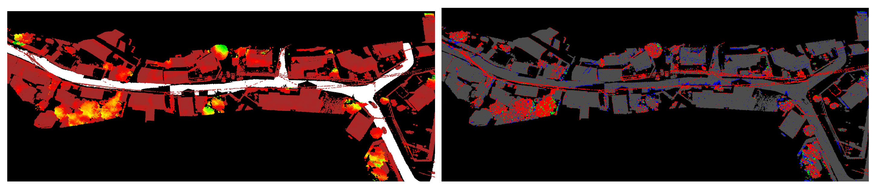
3.2.1. Geometrical Properties

Eigenvaluesare calculated from the covariance matrices of all points in the local neighborhood with the Principal Component Analysis method. For each point, three eigenvalues are obtained. Figure 4 shows the behavior of each of the eigenvalues in a sample urban area.

All eigenvalues are taken into account in this paper, since each one allows us to distinguish between cases of different classes (for example, for eigenvalue 1, low values indicate the class of buildings). Very strong descriptors can be obtained by aggregating all eigenvalues.

Distance to plane refers to the distance between a tested point and a locally fitted plane. The type of plane can vary depending on the scale and point density. It is a very characteristic property of vegetation to have a large amount of noise; hence, the distance to the plane should be higher than with man-made structures.

The aforementioned parameter can be observed in Figure 5. It is clearly visible that trees have a higher variance of distances, but the same can be said about building edges.

Vertical dispersion is a value that corresponds to the amount of noise in a local neighborhood along the Z axis (vertical axis). Vegetation areas have a tendency to be very unstable along the vertical axis, in contrast to urban areas. The example of this feature is presented in Figure 6.

Vertical range computes the distance between the local highest and the local lowest point. It has to be noted that the height range feature from the height-based group features works in exactly the same way, but the difference in the neighborhood provides a vastly different result. In spite of the identical working principle, the vertical range helps to detect objects that are relatively flat along the Z axis; the height range within an infinite cylinder provides information about the local space. For instance, if there are no points above the tested point and the height range is fairly large, it could indicate a powerline cable.

In Figure 7, it can be observed that some power lines, edges of buildings, and most vegetation have higher vertical range values.

Verticality (Figure 8) measures the deviation of the normal vector from the vertical vector.

Vertical objects, such as walls and fences, can be easily distinguished from relatively flat objects such as rooftops. Moreover, many vegetation points are also distinctive, but the most important feature of this property is the ability to discern electrical poles from other more horizontally aligned surfaces such as cables and rooftops.

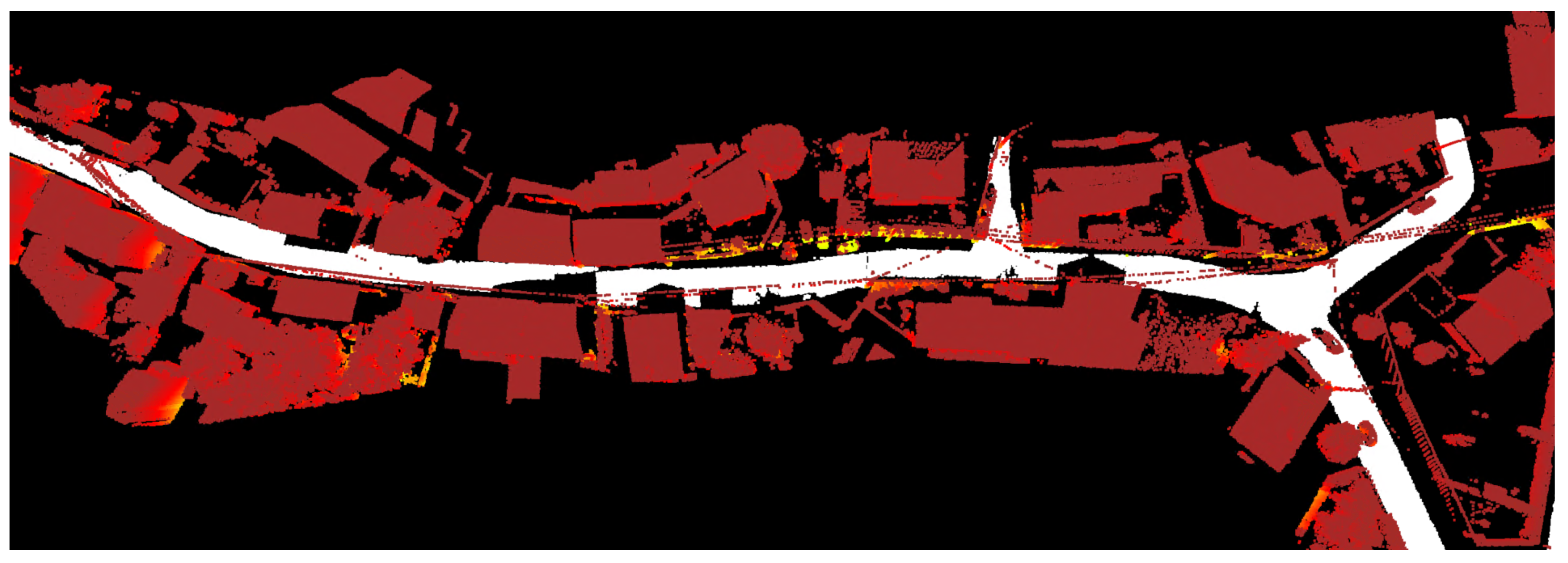
3.2.2. Reflection Properties

Echo scatter measures the number of return dispersions within a local neighborhood. The value reflecting the number of returns is within the <0,3> range, which marks one of the four possible variants described in Section 3.1—single, first, multiple, or last reflection. The purpose of analyzing this value in a local neighborhood is to determine whether it is uniform or scattered. Scattered results indicate vegetation, while a more uniform distribution may point towards man-made objects. For example, most powerline cables consist only of the first echoes, while buildings are almost entirely single echoes, except for the facades.

As depicted in Figure 9, echo scatter showed a significant difference in scattering value on vegetation. However, the accuracy of this feature is degraded due to the penetrating behavior of laser beams. The angle of attack is a very important factor, as slightly increased scattering values on buildings can cause the shadow of catenaries to appear on the roof. Similarly, with regard to vegetation, the echo scatter value tends to increase downwards as the beam passes through the tree and reflects off the branches and the leaves. That usually leaves tree crowns with a relative uniform first echo value as they mark the beginning of the laser beam journey downwards.

Intensity of response indicates the normalized value of response intensity between the various laser scanners.

With the use of response intensity, it is possible to select arbitrary split values at which buildings and catenaries become distinct with different values (see the left part of the Figure 10 versus the right full range part). This implies that since the intensity is normalized for different lasers, it should be possible to find relatively good split values for different types of objects.

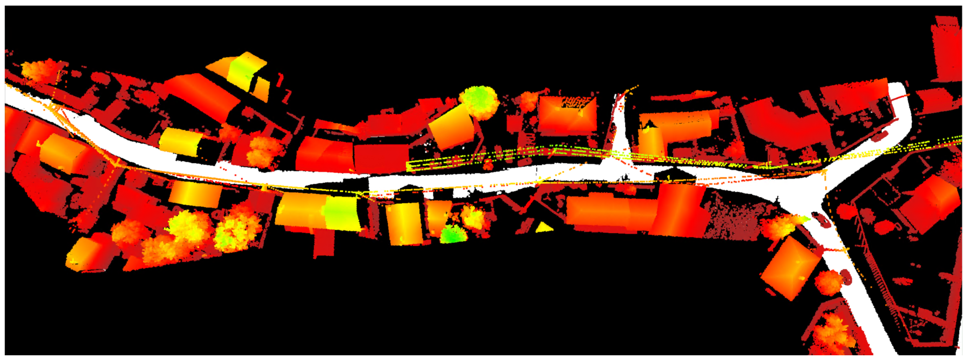
3.2.3. Height Properties

Height above ground estimates the height in meters above the ground, or its interpolation at a point.

Height above ground is an excellent separator for elements of power lines, due to the fact that they cannot appear below four meters above the ground. Figure 11 presents the exact aforementioned effect where power cables clearly appear in brighter colors even towards greens, which represents higher value.

Height range (Figure 12 measures the difference between the minimum and maximum heights relative to the ground within an infinite cylinder. This has been proven to be useful in building detection [1], and due to the KNN height range, it is a strong predictor for power lines. On the other hand, it does not diversify vegetation very well, and consequently, the height above the ground may only be useful when combined with other features.

Height variance indicates a measure within an infinite cylinder variance of the height above the ground values of all points surrounding the tested point (including the tested point).

Height above reflects a distance between the analyzed point and the highest point in the neighborhood, where the height is relative to the ground level estimated locally. Figure 13 shows visible effect on power lines but also to some extent on vegetation and smaller linear objects.

Height above helps to recognize places at the bottom of more complex objects, mostly vegetation. It is also used in the detection of buildings, especially where wall reflections are visible.

Height below reflects the distance between the analyzed point and the lowest point in the neighborhood, where the height is referenced to the locally estimated ground level.

Height below allows to highlight points that define catenaries (see Figure 14). Moreover, it can be useful in distinguishing parts of the vegetation.

3.3. Algorithms

3.3.1. Classical Random Forest

Random forest was selected as one of the algorithms for verification if the features described in the previous subsection were properly prepared for the classification of vegetation, buildings, power lines, and pylons. For the classical random forest approach, the ETZH implementation of random forest contained in the CGAL library was chosen. Due to the specific construction and requirements of the library, the procedure for creating the forest shown in Figure 15 was devised.

Since the number of points in each data pack is quite large and the entire point cloud is characterized by linearity, the input dataset is passed to training in smaller subsets of points. These subsets contain a specified number of segments, where a single segment represents approximately one second of an acquisition flight. A feature vector containing previously described properties is extracted from each of the subsets in the data pack for each of the data points in the cloud, with the class being labeled. A training dataset is created from these feature vectors and is processed by a random forest algorithm. As a result, a defined number of decision trees with the desired maximum depth specified by the user is prepared. All trained trees are then added to the forest.

The process is repeated for every available data pack until all the data is processed. The forests generated for each data pack are merged into one large forest covering all the data, which serves as the final model. Therefore, the size of a model is not constant and depends on the size of the input data and the parameters selected for generating trees. This process is visualized in Figure 16.

3.3.2. XGBoost

The second algorithm, which is taken into account in the experimental session, is XGBoost, since it has recently proved its high effectiveness in many domains. For the XGBoost approach, the size of the forest is controlled by the library due to a different architecture than random forests. XGBoost uses a gradient-boosted trees algorithm. Gradient boosting as a technique has been known for a long time, but the authors of XGBoost [29] based their implementation on Greedy function approximation: a gradient increasing machine. Their model uses a set of classification and regression trees, which gives predictions based on the sum of prediction scores over each tree. The XGBoost model can be described mathematically by the following equation:

$$\widehat{y_i}=\sum _{k=1}^K{f}_k\left(x_i\right),f_k\in ϝ$$

(2)

where K is the number of trees, f is a function in the functional space F, and F is the set of all possible trees.

Therefore, a generalization can be made that XGBoost is still an algorithm that uses tree ensembles as the base approach. The main difference comes in the way in which XGBoost picks new trees and builds forests. Contrary to plenty of standard random forest algorithms, the training does not process the whole forest at once, nor are the features chosen to form a decision randomly. Instead, an additive strategy is used. At each step of the algorithm execution, the progress of forest learning is evaluated, and one more tree is added at a time. The newly added trees are selected to optimize the objective function. The specific objective at step t becomes:

$$\sum _{i=1}^n[g_i{f}_t\left(x_i\right)+\frac{1}{2}{h}_i{f}_t^2\left(x_i\right)]+\Omega \left(f_t\right),$$

(3)

where $g_i$ and $h_i$ are first- and second-order gradient statistics on the loss function, and $\Omega$ penalizes the complexity of the model (i.e., the regression tree functions). That term becomes the optimization goal for the new tree. After applying transformations to the equation, the objective value with the t-th tree is calculated by the following equation:

$$ob{j}^{\left(t\right)}=\sum _{j=1}^T[G_j{\omega }_j+\frac{1}{2}(H_j+\lambda ){\omega }_j^2]+\gamma T,$$

(4)

where:

$$I_j=\left(i\right|q\left(x_i\right))=j,G_j=\sum _{i\in I_j}{g}_i,H_j=\sum _{i\in I_j}{h}_i,$$

(5)

which means that $I_j$ is the set of indices of data points assigned to the j-th leaf, T is a number of leafs, and $\omega$ is a vector of scores on the leaves. $G_i$ and $H_i$ are the sums of first- and second-order gradient statistics, respectively.

4. Experiments

The main objective of the experimental session in the conducted research was to determine the characteristics of individual LiDAR points, which may significantly affect the quality of the point cloud classification to individual classes identified during high-voltage line test flights: buildings, vegetation, power lines, and electric poles. Moreover, the research was also aimed at determining the usefulness of the XGBoost algorithm in the classification of the LiDAR cloud.

The experiments were divided into two separate processes. In the first, we compare two methods:

-

random forests, which are often and commonly used in many classification tasks, including LiDAR point cloud classification.

-

XGBoost, which is one of the best algorithms in the field of classification in various domains, but to the best of the authors’ knowledge, this method has not been used in LiDAR points classification.

The second part of the experiments was devoted to the comparison of the set of features defined in the section concerning the creation of the input dataset, with the leading solutions for feature selection for LiDAR cloud classification:

-

Fuzzy C-Means—A building detection method based on semi-suppressed Fuzzy C-Means and restricted region growing using airborne LiDAR [1].

-

Supervised classification of powerlines—supervised classification of powerlines from airborne LiDAR data in urban areas [23].

-

Contextual classification of point cloud data by exploiting individual 3D neighborhoods [30].

From each of these papers, we have extracted either exactly the same set of features, or their closest resemblances. Every selected feature uses a neighborhood selection of KNN 25; thus, the comparison between the performances of the solutions in the same environment can be made. The sets of all the features for the compared solutions are summarized in

Table 3. Summary of training data and their properties.

Fuzzy C-Means [1]	Cont. Analysis [30]	Supervised Class [23]
Selected features
Change of curvature	-	Change of curvature
Density ratio	-	Density ratio
-	-	Eigenvalues
Height range	Height range	Height range
Height variance	Height variance	-
-	Linearity	Linearity
Omnivariance	Omnivariance	Omnivariance
Planarity	Planarity	Planarity
Sphericity	Sphericity	Sphericity
Point density	Point density	-
-	Sum of eigenvalues	Sum of eigenvalues
-	Verticality	-
-	Anizotropy	-
-	Eigen entropy	-
Distance to plane	-	-
-	Height above ground	-

. The method proposed in this paper uses a set of features listed in Table 2.

In case of the Fuzzy C-Means features [1], the point count ratio and the point density ratio were skipped since they were not applicable in point selection neighborhoods, as described in the paper.

It is worth noting that many of the selected features, e.g., height range, omnivariance, planarity, and sphericity, were chosen in all solutions, or they appear in at least two papers (sum of eigenvalues, point density, height variance, change of curvature, density ratio, and linearity). Moreover, it should be noted that only one algorithm uses an explicit form of eigenvalues, while almost all features are obtained from the previously calculated eigenvalues. Interestingly enough, while all solutions used some form of height analysis, only Wienmann [30] used relative height directly. It should also be said that the solution described in this paper is the only one that uses reflection properties.

4.1. Random Forest Experiments

This section compares the effectiveness of the algorithms described in Section 3.3: Random Forests and XGBoost. The main reason for conducting such experiments is related to the fact that, to the best of our knowledge, XGBoost has not been used in similar studies. To make the model training comparable, both approaches have used the same dataset and feature set. The results obtained during the experimental session are shown in

Table 4. Accuracy and F1 for CGAL random forests and XGBoost.

	CGAL RF		XGBoost RF
	F1	Acc	F1	Acc
vegetation	98.0	96.6	99.4	98.9
buildings	85.7	96.7	96.7	99.1
catenaries	92.2	99.9	89.0	99.8
poles	1.7	99.8	58.0	99.8
overall	69.4	98.3	98.8	99.4

, where the values of the F1 and accuracy measures are summarized.

As should be clearly stated based on the results, XGBoost performs better than the CGAL-based approach. It should be noted that there is one notable exception—in the case of catenaries, the classic CGAL approach performed better both in terms of the F1 score and accuracy. The difference is significant enough to take this solution into account in the case of catenary classification. However, the poles detection level with the use of the CGAL-based implementation is unacceptable. Therefore, in the context of the problem under consideration, XGBoost is more effective. This is also confirmed by the overall measures, where XGBoost reached 98.8% and 99.4% for F1 and accuracy, respectively, while GCAL random forests reached 69.4% and 98.3%. Moreover, most of the time, catenaries and poles are almost always tied together to generate business value. Therefore, hyperparameter tuning for the XGBoost solution will be performed in the next section.

4.2. Hyperparameter Tuning

This section evaluates the main contribution of this paper as a comparison to other solutions for feature selection in the LiDAR classification problem. The experiments were carried out using the Visimind dataset, which was created during acquisition flights in different regions of Europe. A very important feature of the dataset is its versatility in terms of the classification of poles and power lines. This is due to the fact that the flights were made in different geographic conditions in France, Norway, and Romania, which allows for a more general classification than, for example, for a city or for the data from a single region, as in the majority of previous studies. XGBoost was chosen as the algorithm for the evaluation of feature selection, since it turned out to overperform the random forests classifier.

It should also be noted that the choice of the algorithm for the experiments is not crucial, due to the fact that the main goal of the work is to indicate the best possible selection of features for the classification of LiDAR points into the following classes: poles, lines, vegetation, and buildings.

To validate the results, experiments were performed for the previously mentioned parameter selection methods on the same dataset, using exactly the same implementation versions on the same hardware. Additionally, as part of the research with the use of XGBoost, the evaluation was carried out for the following parameter values:

-

Child weight = 1, 2, 4;

-

Number of epochs = 50, 100, 200, max;

-

Depth = 4, 6, 8, 10, 12.

The choices of parameters and their values result from preliminary studies, which showed that the above-mentioned parameters may have an impact on the quality of the classification. In addition, the studies also addressed an assessment of the effectiveness of the classification for various groups of parameters.

Table 5. Accuracy and F1 for Fuzzy C-Means, Cont. Analysis, Sup Class, and our solution.

	Our Solution		Fuzzy C-Means		Cont. Analysis		Sup Class
	F1	Acc	F1	Acc	F1	Acc	F1	Acc
child weight = 1, number of epochs = 100, depth = 6
vegetation	99.2	98.9	98.0	96.6	98.3	97.0	97.3	95.4
buildings	96.8	99.1	89.6	97.2	90.6	97.5	86.7	96.5
catenaries	89.0	99.8	78.4	99.7	93.2	99.9	48.9	99.0
poles	58.0	99.8	22.4	99.6	25.0	99.5	7.3	99.3
overall	98.8	99.4	96.6	98.3	97.0	98.5	95.1	97.6

summarizes the evaluation for our solution and the Fuzzy C-Means, Cont. Analysis, and Sup Class methods.

As can be seen, all methods achieve similar results for vegetation, buildings, and catenaries—only in the case of the Catenaries Sup class is the level of the F1 measure much lower. With respect to the classification of poles, the advantage of our solution is clearly visible, where the F1 measure reaches 58% and significantly exceeds the other methods, which reached 22.4%, 25%, and 7.3%, respectively.

The subsequent experiments taken during the evaluation phase were focused on the impact of the child weight parameter on classification effectiveness. The results for different levels of this parameter are presented in

Table 6. F1 and accuracy for different child weight levels.

	Our Solution		Fuzzy C-Means		Cont. Analysis		Sup Class
	F1	Acc	F1	Acc	F1	Acc	F1	Acc
child weight = 2
vegetation	99.4	98.9	98.0	96.6	98.3	97.0	97.3	95.5
buildings	96.7	99.1	89.5	97.2	90.6	97.5	86.7	96.5
catenaries	89.0	99.8	78.4	99.7	93.0	99.9	49.0	99.08
poles	58.5	99.8	22.5	99.6	25.5	99.5	7.7	99.3
overall	98.8	99.4	96.5	98.3	97.0	98.5	95.2	97.6
child weight = 4
vegetation	99.2	98.6	98.0	96.6	98.3	97.0	97.3	95.5
buildings	95.9	98.9	89.5	97.2	90.5	97.5	86.7	96.5
catenaries	86.6	99.8	78.4	99.7	93.1	99.9	48.8	99.0
poles	46.4	99.7	22.3	99.6	25.2	99.5	7.1	99.3
overall	98.5	99.3	96.5	98.3	97.0	98.5	95.2	97.6

.

Deviating from the default child weight setting does not significantly affect the results. Increasing the child weight parameter to 2 and to 4 slightly increases the effectiveness of the considered algorithms only in individual cases. On the other hand, there are also many cases where the obtained results are much worse (for example, in our contribution for child weight equal to 4, the F1 measure decreased for the poles class to 46.4%). Therefore, a child’s weight of 1 was found to be optimal.

The next step of the research was to check the effects of different tree depths on the F1 and accuracy values. The summarization data is presented in

Table 7. F1 and accuracy for different depth levels.

	Our Solution		Fuzzy C-Means		Cont. Analysis		Sup Class
	F1	Acc	F1	Acc	F1	Acc	F1	Acc
depth = 4
vegetation	99.2	98.6	97.6	96.3	98.0	96.7	97.4	95.5
buildings	95.9	98.9	88.5	96.9	89.5	97.2	86.7	96.5
catenaries	86.6	99.8	75.7	99.6	92.5	99.9	47.5	99.0
poles	46.4	99.7	19.4	99.6	20.8	99.5	5.9	99.3
overall	98.5	99.3	96.2	98.1	96.6	98.3	95.1	97.6
depth = 8
vegetation	99.5	99.1	98.2	96.9	98.4	97.2	97.4	95.5
buildings	97.4	99.3	90.2	97.4	91.0	97.6	87.0	96.6
catenaries	91.5	99.9	80.2	99.7	94.0	99.9	49.5	99.0
poles	71.3	99.9	30.1	99.6	31.7	99.6	9.6	99.4
overall	99.1	99.6	96.8	98.4	97.2	98.6	95.3	97.6
depth = 10
vegetation	99.6	99.4	98.3	97.0	98.5	97.5	97.5	95.6
buildings	98.0	99.5	90.8	97.6	91.8	97.8	87.4	96.6
catenaries	93.9	99.9	82.0	99.7	94.8	99.9	51.1	99.1
poles	81.8	99.9	37.2	99.7	40.4	99.7	12.6	99.4
overall	99.4	99.7	97.0	98.5	97.5	98.7	95.4	97.7
depth = 12
vegetation	99.7	99.5	98.4	97.3	98.6	97.7	97.5	95.7
buildings	98.4	99.6	91.2	97.7	92.2	97.9	87.4	96.6
catenaries	94.7	99.9	83.4	99.8	95.5	99.9	52.0	99.1
poles	85.4	99.9	47.6	99.7	50.0	99.7	17.6	99.4
overall	99.5	99.7	97.2	98.6	97.6	98.8	95.5	97.7

.

Modifying the maximum depths of individual trees produces significant changes in the results. The default parameter of 6 does not achieve the best results. An increase in the effectiveness of the solutions can be observed with each degree of depth increase. This is especially visible in the case of the F1 measure for the poles class, which was the most difficult to classify. Increasing the depth of trees can lead to an overfitting problem, which can be difficult to detect. This is due to the fact that although the test data was previously invisible to the training algorithm, it is still taken from the same region as part of the training data, and represents similar geometry, point density, and terrain characteristics. However, the algorithm has been trained on three different regions of the world, and so it is likely that overfitting does not occur. Another problem is training time, which increases significantly with increasing tree depth. This can be a problem, especially when trying to mitigate the problem of overfitting by increasing the total number of trees that are averaged.

The last part of the experiments focused on checking the effect of changing the number of epochs on the quality of individual algorithms. It should be noted that the number of epochs is exactly the same as the number of trees used in XGBoost, since each step of the algorithm causes a new tree to be added. Moreover, assuming the level of the parameter as being maximum, the final number of epochs will be different for each of the algorithms. This is due to the fact that in each case, an appropriate effectiveness will be achieved in a different number of steps. The obtained results are summarized in

Table 8. F1 and accuracy for different numbers of epochs.

	Our Solution		Fuzzy C-Means		Cont. Analysis		Sup Class
	F1	Acc	F1	Acc	F1	Acc	F1	Acc
epochs = 50
vegetation	99.2	98.7	98.0	96.5	98.2	96.9	97.3	95.4
buildings	96.1	99.0	89.0	97.0	90.0	97.4	86.6	96.4
catenaries	87.4	99.8	77.0	99.6	92.8	99.9	48.7	99.0
poles	49.0	99.7	19.9	99.6	21.6	99.5	5.7	99.3
overall	98.6	99.3	96.4	98.2	96.8	98.4	95.1	97.6
epochs = 200
vegetation	99.5	99.1	98.1	96.8	98.4	97.2	97.4	95.5
buildings	97.3	99.3	90.0	97.4	91.0	97.6	86.9	96.5
catenaries	90.9	99.9	79.6	99.7	93.5	99.9	49.3	99.0
poles	68.9	99.9	26.4	99.6	30.2	99.6	9.8	99.4
overall	99.0	99.5	96.7	98.4	97.2	98.6	95.2	97.6
epochs = max
	max = 563		max = 612		max = 451		max = 384
vegetation	99.7	99.4	98.3	97.1	98.5	97.4	97.4	95.6
buildings	98.2	99.5	90.8	97.6	91.6	97.8	87.0	96.6
catenaries	93.8	99.9	81.4	99.7	94.5	99.9	50.0	99.1
poles	81.9	99.9	39.4	99.7	39.3	99.7	13.0	99.4
overall	99.4	99.7	97.0	98.5	97.4	98.7	95.3	97.7

, where the number of epochs for each algorithm execution is pointed out as well.

As can be deduced from the summary of the algorithms’ executions, all solutions achieved much better results with an increase in the number of trees. However, adding more trees makes the inference time significantly slower, which can make the models ineffective. When comparing the training times of the models for the default value of 100 trees and for the maximum number of epochs, it appears that with 100 trees, the training time is 3.8 to 6.1 times lower. In conclusion, it should be noted that the optimization of the number of epochs, as in the case of tree depth, significantly extends the training time.

Additionally, the conducted experiments show that the authors’ set of features prepared in this publication achieves much better results than the leading solutions regarding the selection of features in the problem of classification of buildings, vegetation, catenaries, and poles. Particularly large differences are evident in the case of the F1 parameter, where our solution exceeds the level of 85%, and the best result for the other solutions allows us to reach a maximum of 50%.

5. Conclusions

In this study, a new approach for feature selection in the LiDAR data classification problem was proposed. As part of the work, the features belonging to the following three groups were identified: geometrical, height-based, and reflection property-based. Most of them were also identified in similar studies, but the elements based on laser internal properties and height-relative features were only included in this paper. During the evaluation, they proved to be highly effective, even in classifying the classes containing a relatively small number of elements. For evaluation, leading machine learning algorithms were chosen, namely, random forests and XGBoost. Our solution has been compared with the research on the selection of features in similar classification problems. It turned out that the proposed method overperformed all other solutions, reaching an overall accuracy of 99%, as well as for each of the four classes separately. Moreover, in terms of the F1 measure, our solution reached 98 % for buildings and vegetation, 93% for catenaries, and 81% for poles. The largest difference was observed within the F1 measure for poles, where the related works showed the level of this measure at a maximum of 50%.

Future research will be extended to additional features during evaluation. Research will also be directed to thoroughly checking on the impacts of individual model parameters on training time. Finally, other machine learning models, particularly those based on deep learning, will be implemented to evaluate LiDAR point cloud classification.