Article

Feature Scalar Field Grid-Guided Optical-Flow Image Matching for Multi-View Images of Asteroid

1
School of Environment and Spatial Informatics, China University of Mining and Technology, Xuzhou 221116, China
2
School of Computing and Mathematics, College of Science and Engineering, University of Derby, Derby DE22 1GB, UK
3
Shandong Province Institute of Land Surveying and Mapping, Jinan 250013, China
4
Shandong Zhengyuan Aerial Remote Sensing Technology Co., Ltd., Jinan 250101, China
*
Author to whom correspondence should be addressed.
Remote Sens. 2023, 15(24), 5786; https://doi.org/10.3390/rs15245786
Submission received: 1 September 2023 / Revised: 14 December 2023 / Accepted: 16 December 2023 / Published: 18 December 2023

Abstract

:
Images captured by deep space probes exhibit large-scale variations, irregular overlap, and remarkable differences in field of view. These issues present considerable challenges for the registration of multi-view asteroid sensor images. To obtain accurate, dense, and reliable matching results of homonymous points in asteroid images, this paper proposes a new scale-invariant feature matching and displacement scalar field-guided optical-flow-tracking method. The method initially uses scale-invariant feature matching to obtain the geometric correspondence between two images. Subsequently, scalar fields of coordinate differences in the x and y directions are constructed based on this correspondence. Next, interim images are generated using the scalar field grid. Finally, optical-flow tracking is performed based on these interim images. Additionally, to ensure the reliability of the matching results, this paper introduces three methods for eliminating mismatched points: bidirectional optical-flow tracking, vector field consensus, and epipolar geometry constraints. Experimental results demonstrate that the proposed method achieves a 98% matching correctness rate and a root mean square error of 0.25 pixels. By combining the advantages of feature matching and optical-flow field methods, this approach achieves image homonymous point matching results with precision and density. The matching method exhibits robustness and strong applicability for asteroid images with cross-scale, large displacement, and large rotation angles.

1. Introduction

Asteroid exploration holds considerable importance in studying the origin of the solar system and predicting asteroid impact events on Earth [1,2]. It is currently a key direction and research hotspot in deep space exploration, following lunar and Mars missions [3]. Obtaining high-resolution terrain information on the surface of an asteroid is a prerequisite for autonomous navigation and safe landing of the probe [4] and crucial for asteroid exploration missions [5]. Accurate and high-density image matching results are prerequisites for generating 3D shapes with high geometric accuracy and model refinement in asteroid exploration missions [6,7]. However, due to the limited texture of the asteroid and the limited presence of topographical features [8], along with the weak gravity of the asteroid, the images acquired by the probe exhibited huge differences in shooting angle and resolution. These characteristics of asteroid images pose considerable challenges for the dense matching of multi-view images [4].
To obtain homonymous points in multiple images with large-scale changes, scale-invariant feature-matching methods, such as SIFT [9] and SURF [10], have been proven to be reliable, and they are often used in asteroid shape reconstruction. Cui et al. [11] used the PCA-SIFT [12] algorithm to match feature points in sequential images taken during the Eros flyby phase, successfully achieving feature tracking in situations with the image field of view changes. In the process of 3D reconstruction of Vesta using sequence images, Lan et al. [13] obtained reliable homonymous points based on SIFT matching and combined them with methods such as sparse bundle adjustment to obtain accurate position and attitude parameters of sequence images. Liu et al. [14] used SIFT matching in the structure from motion method to ensure the reliability and robustness of homonymous point matching to solve the image matching and high-precision 3D modeling problems of weakly textured asteroids. SIFT matching exhibits strong robustness in different scenarios and can be used as a constraint for other image-matching methods. However, scale-invariant feature-matching algorithms, such as SIFT, also have their drawbacks. For instance, the homonymous points obtained by these methods are relatively sparse and may not fully meet the requirements for obtaining detailed 3D information on asteroids.
Optical-flow methods have proven effective in utilizing the grayscale information of images. Since the inception of the Lucas–Kanade (LK) [15] optical-flow algorithm in 1981, image alignment based on optical flow has found widespread applications in diverse fields such as computer vision, autonomous driving, medicine, and industry [16,17,18]. By fully utilizing the grayscale information of images, optical-flow methods enhance the density of multi-view image-matching points. In recent years, researchers have explored the application of optical-flow fields for homonymous point matching in deep space exploration images. Debei et al. [19] utilized optical-flow algorithms to refine the matching results to sub-pixel levels during the 3D reconstruction of asteroids based on multi-view images. Chen et al. [20] applied optical-flow estimation to the registration of Chang’e-1 multi-view images, achieving sub-pixel matching accuracy of Lunar images. Despite the ability to generate dense image-matching results, optical-flow methods rely on strong assumptions of small displacement and grayscale invariance, leading to limitations in practical applications. Although substantial advancements have been made in optical-flow methods over the past few decades, large displacement optical-flow estimation remains a challenge to be addressed in asteroid image-matching scenarios [21,22]. To address the limitations of optical-flow tracking in large displacement and multi-scale scenarios, some researchers have introduced image feature-based matching algorithms, such as SIFT, as prior conditions. Brox and Malik [22] integrated feature matching into the optical-flow framework, enabling the satisfactory capture of non-rigid large displacement motion. Liu et al. [23] calculated the homography matrix based on Harris–SIFT matching points and utilized it to guide the LK optical-flow method in finding local optimal matching points, resulting in more accurate matching results. Wang et al. [24] added SIFT feature matching as a constraint term to the energy function, successfully achieving registration of large deformation medical images based on optical-flow fields. To solve the problem of large displacement optical-flow estimation, Wang et al. [25] proposed a feature matching-based optical-flow optimization algorithm. This approach integrates feature matching into the variational optical-flow framework, fully leveraging the robustness of feature matching under large displacement conditions and the density of variational optical flow.
The aforementioned research underscores the efficacy of algorithms with strong scale adaptability, such as SIFT, in providing reliable preliminary conditions for optical-flow methods. In addition to contending with large displacement and significant scale variations, asteroid images encompass considerable rotation angles and uneven scale deformation. These complexities compound the challenge of optical-flow tracking, and existing techniques struggle to concurrently address these issues. Furthermore, research on image homologous point matching based on optical-flow fields for asteroid images remains limited, necessitating further exploration of the potential benefits of optical-flow methods. To address these gaps, this paper capitalizes on the unique characteristics of asteroid images, merging the strengths of feature matching and optical-flow field methods. It presents an asteroid multi-view image-matching approach grounded in feature-guided optical-flow tracking, with the aim of attaining accurate and densely populated homologous point-matching results for asteroid images. This method incorporates the SIFT matching algorithm within the optical-flow tracking process, leveraging the robustness of feature-matching techniques to impart constraint conditions for optical-flow tracking in challenging scenarios. Introducing a novel approach centered on scalar field grids in the x and y directions, the method guides optical-flow tracking, notably enhancing the accuracy of initial parameter values to be solved. The optical-flow tracking process is further streamlined by introducing intermediate images, a strategy that mitigates the intricacies of optical-flow tracking and augments algorithmic robustness. In all, this approach effectively addresses the limitations of optical-flow fields in scenarios marked by cross-scale disparities, substantial displacement, and extensive rotation angles.

2. Methods

2.1. Problem Definition

Due to the weak gravity of the asteroid, the challenges of accurately controlling the attitude of the probe, and the significant changes in the probe’s orbit, the images captured by the sensor exhibit distinct characteristics, such as large-scale variations, irregular overlaps, and significant differences in shooting angles. Although optical-flow-based homonymous point tracking offers advantages, such as high density and fast processing speed, it demands strict prerequisite conditions. Specifically, the optical-flow tracking algorithm must satisfy two fundamental hypotheses.
Hypothesis 1:
The brightness constancy assumption or the gray level invariance assumption means that the brightness of the same point remains unchanged at different times.
Hypothesis 2:
The small motion assumption, which means that the change in the same point with time will not cause considerable changes in position.
These two assumptions are required, and in most cases, the asteroid images acquired by the probe cannot directly use the optical-flow method for image matching. Therefore, when using the optical-flow method for asteroid image matching, these issues must be addressed. Based on these two basic assumptions, the mathematical model of the optical-flow method can be defined using the following formulas.
Assuming that I(x, y, t) is the pixel value (gray value) of the pixel point whose coordinates are (x, y) in the previous image at time t, the coordinate of the pixel point in the next image at time t + Δt is (x + Δx, y + Δy). Based on Hypothesis 1:
I x , y , t = I x + x , y + y , t + t .  
Based on Hypothesis 2, Taylor series expansion is performed on the right part of Equation (1):
I x + x , y + y , t + t = I x , y , t + I x x + I y y + I t t   + .
From Equations (1) and (2), we yield:
I x x + I y y + I t t = 0 .
From Equation (3):
I x x t + I y y t = I t .  
Let:
x t = u ; y t = v ; I x = I x ; I y = I y ; I t = I t ;
I x I y u v = I t .  
Equation (5) contains two unknowns and cannot be solved using only one point. For this problem, the Lucas–Kanade optical-flow algorithm proposed the third hypothesis [26].
Hypothesis 3:
The motion of adjacent pixels is consistent.
Based on Hypothesis 3, Equation (5) can be extended to:
I x 1 I x 2 I x 3 I x n I y 1 I y 2 I y 3 I y n u v = I t 1 I t 2 I t 3 I t n .
In Equation (6), 1, 2, 3, …, n is the index number of the neighboring pixels of the center pixel. Equation (6) is an overdetermined system of equations, which can be solved using the least squares method.
Optical-flow-tracking algorithms are widely used in object tracking in video images, mainly due to the strong continuity of video images. However, satisfying the second assumption, which is small motion, is difficult for the asteroid images. From the perspective of pixel positions in the image, two asteroid images with overlapping areas may encounter the following:
(1)
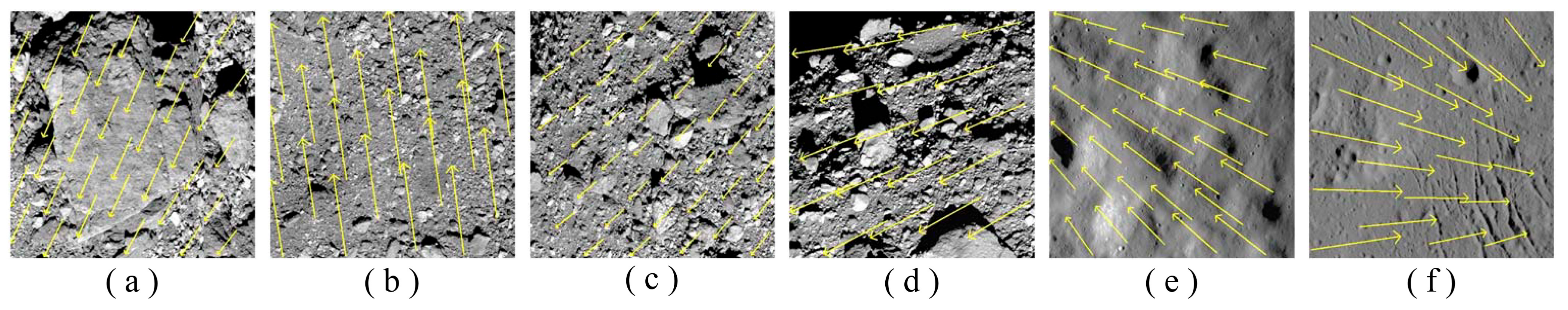
Pixels have large position changes.
(2)
Pixels have large rotation angles, as well as different movement amounts because of the varying distances between pixels and the image rotation center.
(3)
Large-scale changes of adjacent pixels caused by different distances and shooting angles of the camera center relative to the shooting area.
The issues arising from these three scenarios are significantly more intricate than those arising from the small motion assumption, and conventional techniques are inadequate to address these issues. This paper focuses on solving the problem wherein asteroid images cannot satisfy the second assumption.

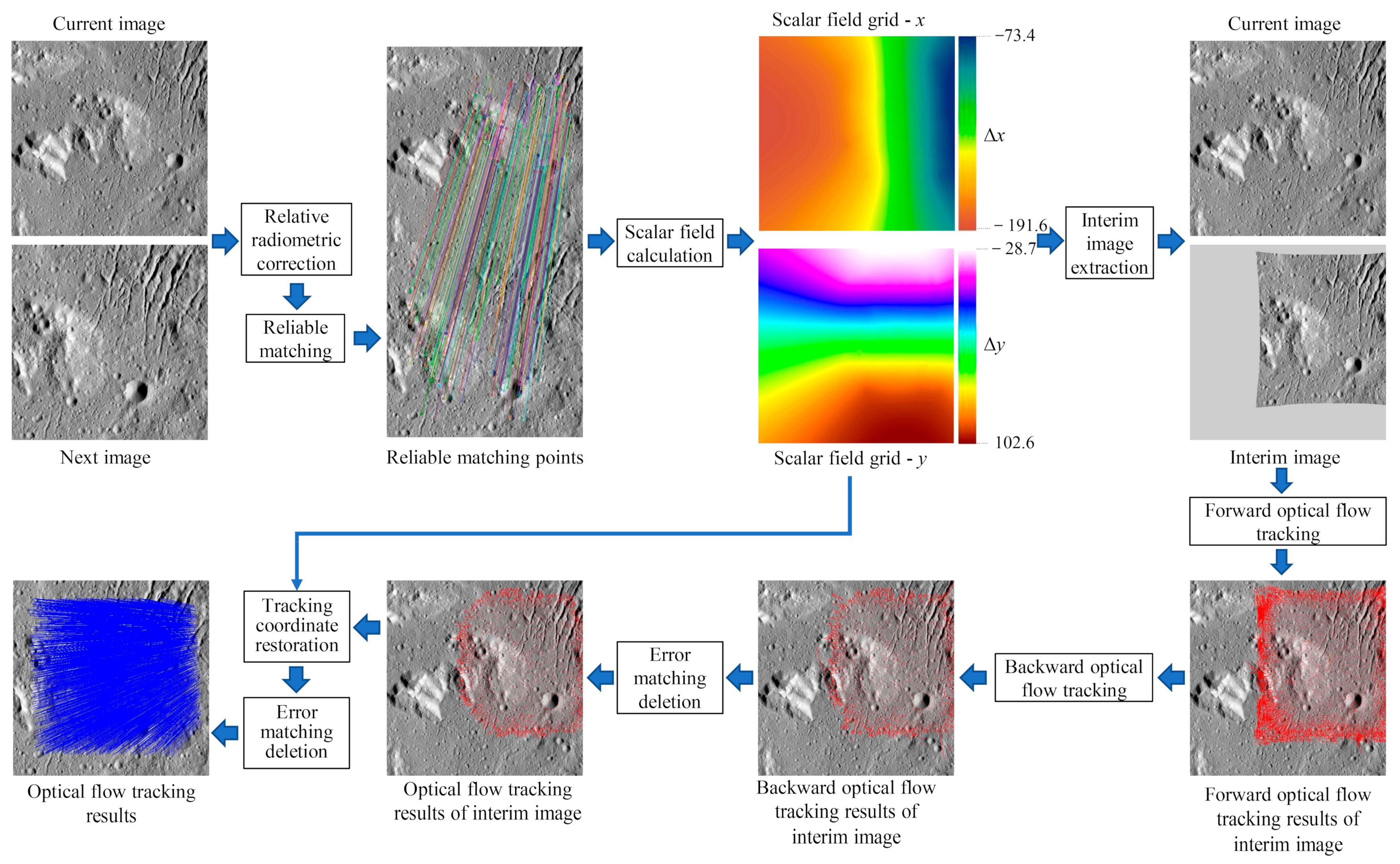
2.2. Improved Optical-Flow-Tracking Algorithm

To address the aforementioned issues, this paper introduces a novel optical-flow tracking method guided by scale-invariant feature matching and displacement scalar fields. The core concept is to begin by acquiring reliable homonymous matching points via the scale-invariant feature-matching algorithm. With the aim of ensuring accuracy and smoothness in the pixel mapping relationship between the two images, x and y directional displacement scalar field grids are constructed based on the reliable matching points. Subsequently, the mapping relationship is derived from the x and y directional scalar field grids, leading to the construction of interim images. Optical-flow tracking is then performed through these interim images, effectively resolving the three types of issues commonly encountered in asteroid images. Moreover, the proposed method combines epipolar geometry constraints, forward and backward optical flows, and vector field consensus (VFC) techniques to eliminate erroneous matches at multiple stages, further enhancing the robustness of the process. Finally, the optical-flow tracking coordinates are restored using the x and y directional displacement scalar field grids.
The algorithm process includes nine main steps, as shown in Figure 1. In the following sections, we will elaborate on the key steps of scalar field grid construction, interim image extraction, optical-flow tracking, and erroneous match elimination.

2.3. Scalar Field Grid Construction and Interim Image Extraction

2.3.1. Scalar Field Grid Construction

Accurate and evenly distributed homonymous matching points play a crucial role in establishing the pixel mapping relationship between two images. To achieve this goal, a robust method is necessary. The SIFT descriptor, which can effectively capture the position, scale, and orientation information, expressing the feature vector of key-points through 128 gradient values [27], is employed in this paper. SIFT possesses several advantages, such as scale invariance, rotation invariance, viewpoint invariance, affine transformation invariance, and brightness invariance. Given that the brightness difference of sequential images can impact the accuracy of tracking points, we introduced a relative radiation correction algorithm before SIFT matching to ensure that the brightness space of multiple images is relatively uniform. In this paper, SIFT feature matching is used as the foundation for obtaining homonymous points in the two images, and the process consists of four main steps:
(1)
Detect key-points in the image and extract the SIFT feature descriptors of these key-points.
(2)
Use a fast nearest-neighbor search algorithm to obtain matching relationships.
(3)
Combine the random sample consensus (RANSAC) [28] algorithm and the fundamental matrix to eliminate erroneous matching point pairs.
(4)
Remove overlapping points or points with close distances.
In this paper, the homonymous matching point pairs obtained from the two images are referred to as reliable matching point pairs. Based on these reliable matching point pairs, scalar field grids are constructed in the x and y directions. The construction of the scalar field grid needs to consider the spatial correlation, accuracy, and smoothness requirements of the homonymous matching points. As such, the Ordinary Kriging interpolation algorithm is employed. This algorithm involves three main steps:
(1)
Based on the x and y coordinate pairs of homonymous points in the two images, the difference in x and y coordinates for each point is calculated (i.e., Δx and Δy).
(2)
Based on xi, yi, Δxi (i = 1,2, 3,…,n), the Ordinary Kriging interpolation algorithm is used to generate a raster file with the same size and resolution as the initial image, which is the x-direction scalar field grid.
(3)
Based on xi, yi, Δyi (i = 1,2, 3,…,n), the Ordinary Kriging interpolation algorithm is used to generate a raster file with the same size and resolution as the initial image, which is the y-direction scalar field grid.

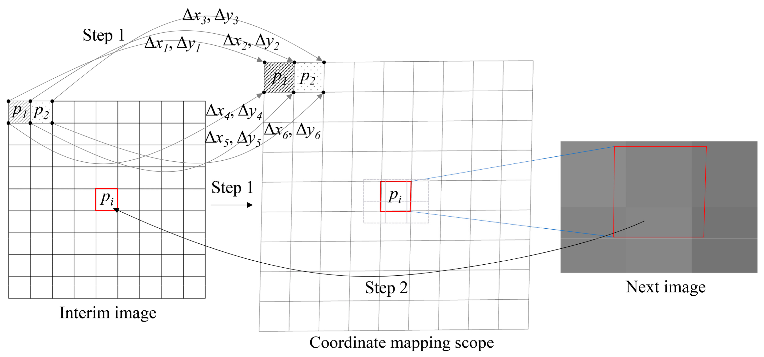
2.3.2. Interim Image Extraction

The extraction of interim images serves two main objectives: first, to preserve the grayscale information of the initial image, and second, to retain the gradient information without any loss. To achieve these objectives, this paper proposes a method for extracting interim images, outlined in Figure 2. The method involves determining the value of each pixel in the interim image through two steps. In the first step, the corresponding coordinates of the four corner points of the pixel in the next image are calculated. This step provides the value scope of the pixel on the next image based on the scalar field grid in the x and y directions. In the second step, the pixels covered by the calculated value scope in the next image are determined. Subsequently, the pixel values of the interim image are calculated using Equation (7).
I i , j = c = 1 n I c × A c A i , j ,
where Ii,j represents the pixel value of the interim image, Ai,j represents the area of the value scope, n is the number of pixels in the next image covered by the value scope, I′c represents the grayscale value of the pixel c, and A′c represents the area of the pixel c covered by the value scope.
Figure 2. Mapping relationship of interim image pixel’s extraction. Δx and Δy are obtained based on a scalar field grid in the x and y directions, respectively. Pixel pi obtains coordinate mapping values for the four corners through Δx and Δy. The grayscale values are taken at the corresponding scope on the next image based on the mapped coordinate values of the four corners of pixel pi.
Remotesensing 15 05786 g002
The proposed method for extracting pixel values of interim images ensures that no gaps or overlaps exist in the value scope mapped onto the initial image (i.e., the next image). This process establishes a unique correspondence between the pixels of the initial image and the interim image. By using this mapping method, the initial grayscale information can be fully reflected in the interim image while preserving the gradient trend of the initial image.

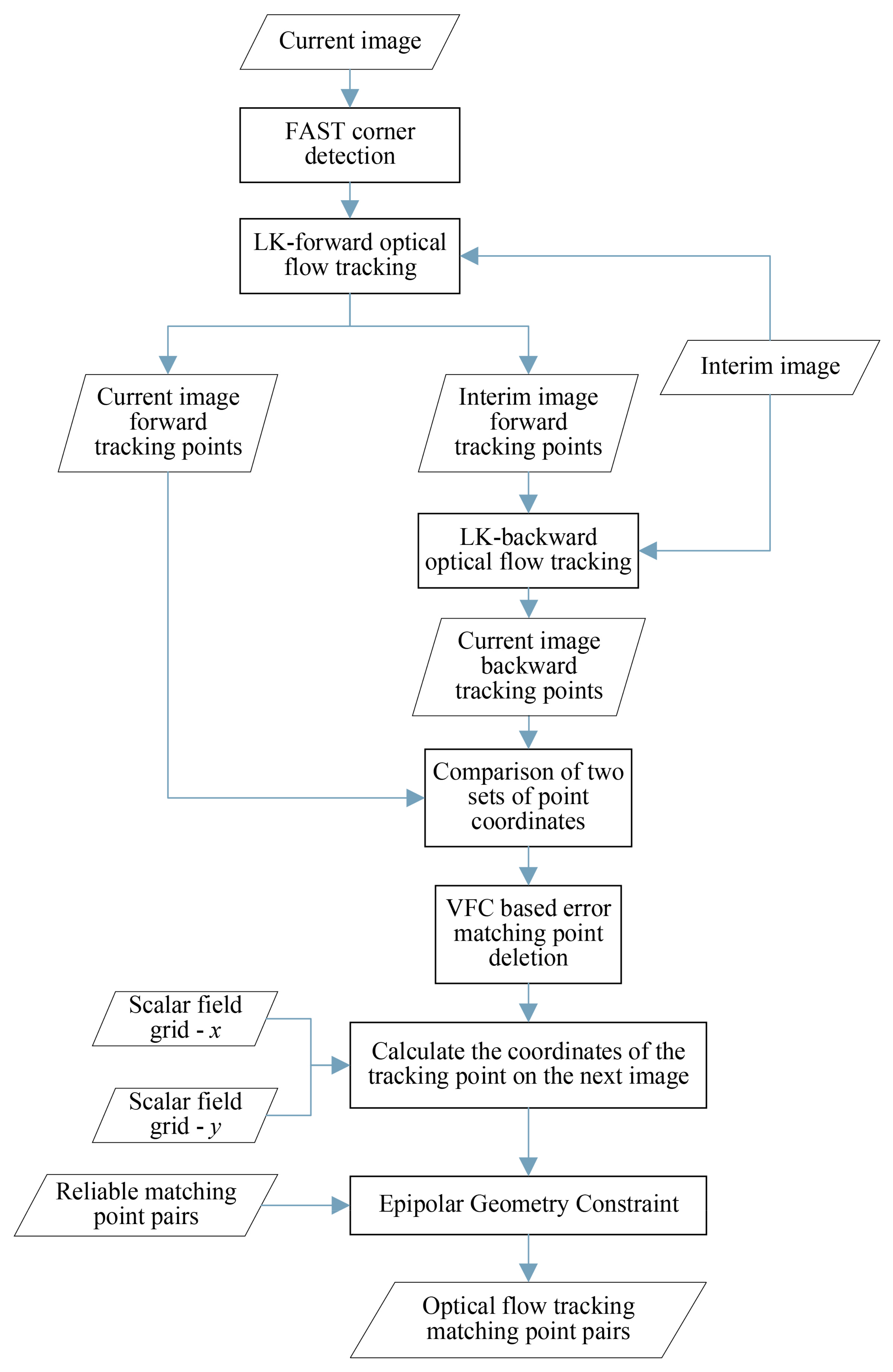
2.4. Optical-Flow Tracking

The fundamental principle of optical-flow tracking is to identify the correspondence between pixels in adjacent images by utilizing the gradient value and its changing trend of pixels at the same position in the image sequence. The necessary premise of the optical-flow algorithm is that the displacement value of the pixels in the previous frame and the next frame of the image is very small so the gradient information is useful. In optical-flow tracking, the difference in grayscale information between two frames of images can be used as the objective function. In the optical-flow-tracking process, the correspondence between pixels can be obtained through multiple iterations. The objective of optical-flow tracking is to establish the correspondence between homonymous matching points in two images. To achieve this objective, the method proposed in this paper is divided into seven steps, as depicted in Figure 3, to obtain the coordinate values of homonymous matching points between the current image and the next image.
(1)
The first step involves the extraction of feature corner points. When observing the motion of an object, the local motion information within the observation window is limited due to the window’s size. As a result, accurate tracking of motion along the image gradient within the observation window, such as object edges, becomes challenging. This phenomenon is known as the aperture problem [29]. Additionally, optical-flow tracking can be inaccurate in areas with uniform texture. To ensure accurate tracking results, feature points must be extracted from the image before performing optical-flow tracking. In this paper, the features from the Accelerated Segment Test (FAST) algorithm [30] are employed to extract feature corner points from the current image, forming Coordinate Point Set 1.
(2)
Based on Coordinate Point Set 1, obtained in the first step, the coordinates of each point on the interim image were estimated one by one, resulting in the forward-tracking results denoted as Coordinate Point Set 2. These coordinates represent the points that can be successfully tracked in the interim image. After this step, Coordinate Point Set 1 is updated to reflect the new set of points used for tracking. Furthermore, record the correspondence between homonymous points in Coordinate Point Sets 1 and 2.
(3)
Based on the Coordinate Point Set 2 obtained in the second step, the coordinates of each point on the current images were estimated one by one. This process is known as backward tracking and results in Coordinate Point Set 3. Additionally, record the correspondence between homonymous points in Coordinate Point Set 2 and Coordinate Point Set 3.
(4)
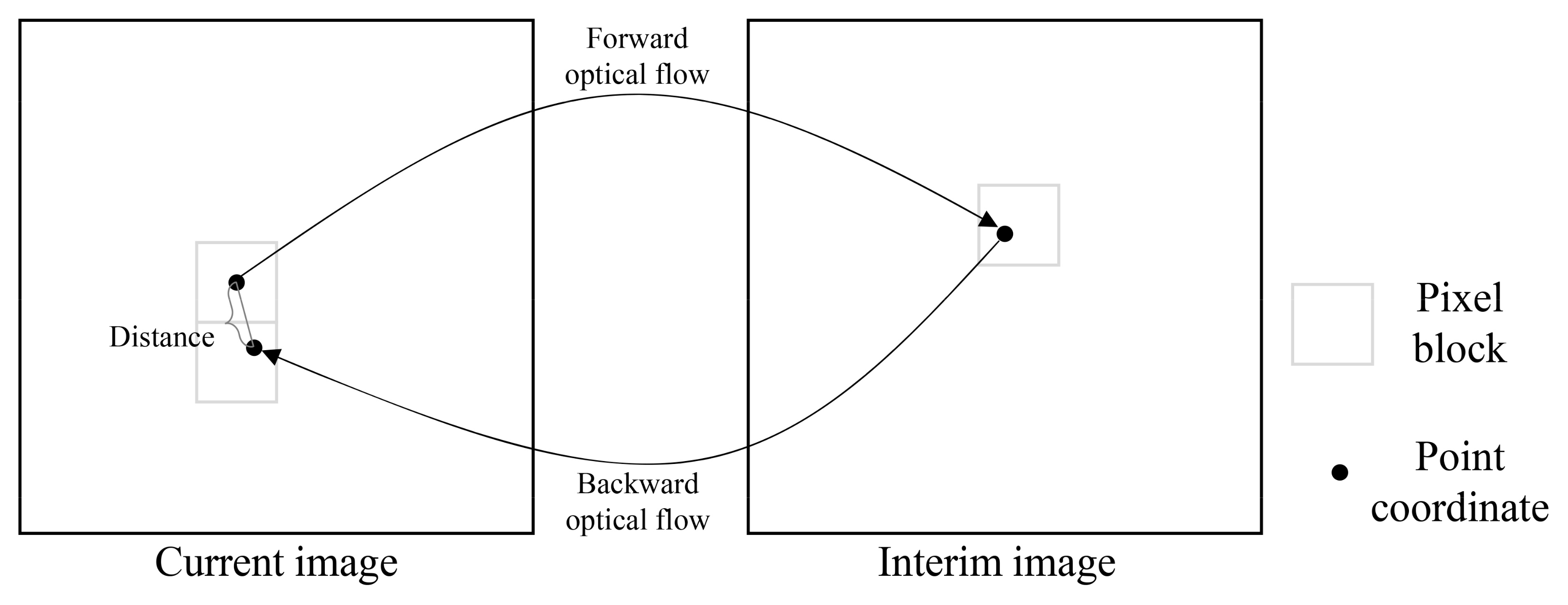
Calculate the Euclidean distance between the homonymous points in Coordinate Point Set 1 and Coordinate Point Set 3, as illustrated in Figure 4. If the distance is less than the specified threshold, then the optical-flow tracking result is deemed accurate, and the matching point pairs are retained. Conversely, if the distance exceeds the threshold, then the result is considered incorrect, and the erroneous matching point pairs are removed. In this paper, the distance threshold is set to 1 pixel. After this step, Coordinate Point Sets 1 and 2 are updated with the refined and accurate matching point pairs.
Figure 4. Schematic diagram of bidirectional optical-flow tracking.
Remotesensing 15 05786 g004
(5)
Using the matching-point pairs verified by forward and backward optical-flow tracking, which are the results obtained in the fourth step, apply the vector field consensus algorithm to further eliminate erroneous matching point pairs. After this step, update Coordinate Point Sets 1 and 2.
(6)
Based on Coordinate Point Set 2, calculate the coordinates of each point on the next image one by one using Equations (8) and (9). This process involves restoring the tracking coordinates, and the resulting coordinates are denoted as Coordinate Point Set 4.
X x , y = x + w 0 × X G x , y + w 1 × X G x , y + 1 + w 2 × X G x + 1 , y   + w 3 × X G x + 1 , y + 1 ,  
Y x , y = y + w 0 × Y G x , y + w 1 × Y G x , y + 1 + w 2 × Y G x + 1 , y   + w 3 × Y G x + 1 , y + 1 ,  
where w 0 = 1 x + x × 1 y + y , w 1 = 1 x + x × y y , and w 2 = x x × 1 y + y , w 3 = x x × y y . x and y are the vertical and horizontal coordinates of the interim image, respectively; X(x, y) and Y(x, y) are the vertical and horizontal coordinates on the next image, respectively; x′ and y′ are the integer parts of x and y values, respectively; and XG(x′, y′) and YG(x′, y′) are the grid values of the scalar field grid in the x and y directions of the x′ row and y′ columns, respectively.
(7)
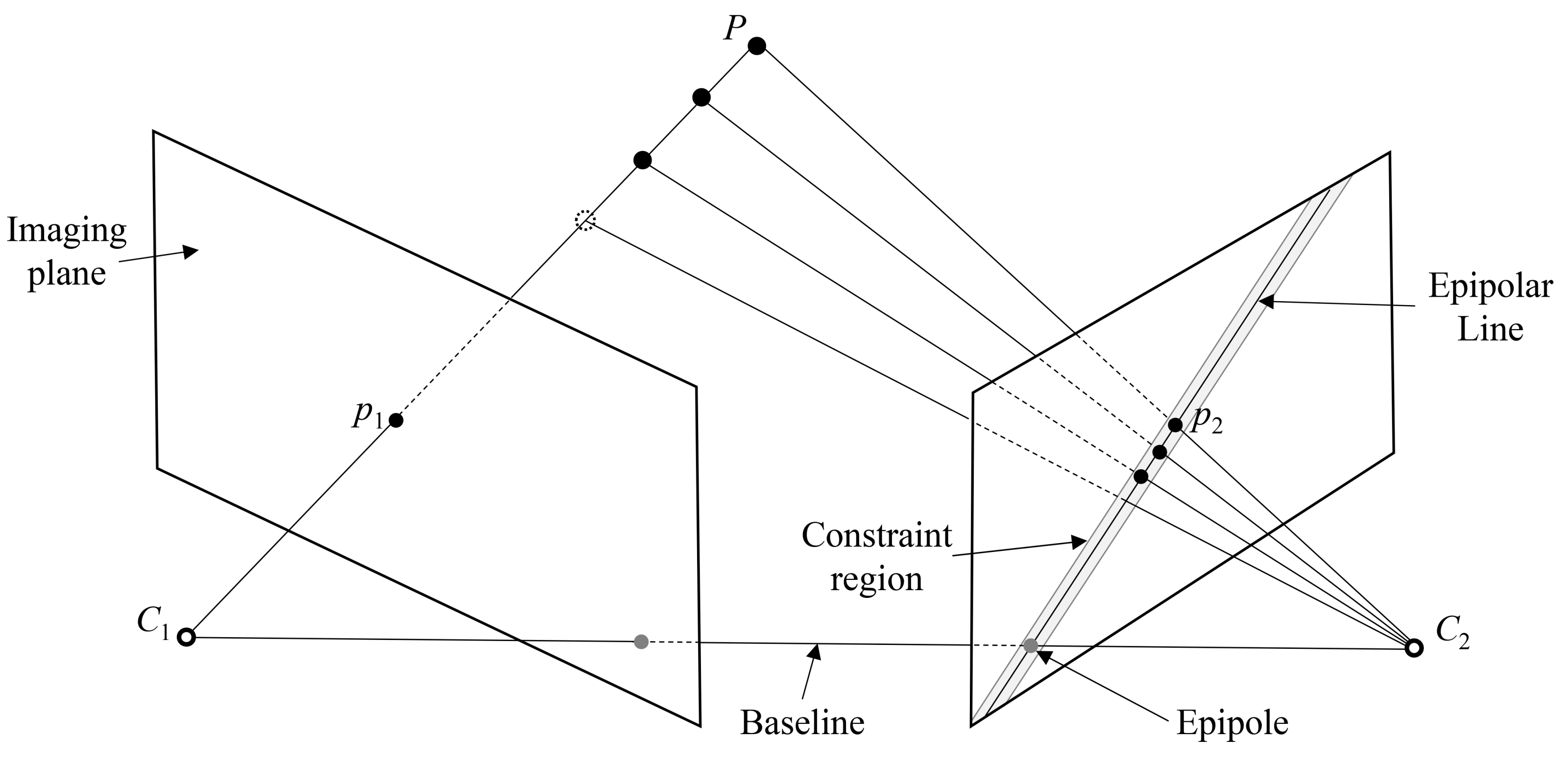
Using the reliable matching point pairs obtained in Section 2.3.1, calculate the fundamental matrix between the current image and the next image. Utilizing this fundamental matrix, compute the epipolar lines for all points in Coordinate Point Set 1 in the next image and record the correspondence between the points and their respective epipolar lines. Subsequently, calculate the Euclidean distance from each point in Coordinate Point Set 4 to its corresponding epipolar line individually. If the distance exceeds the threshold, then the point is considered an erroneous matching point, as illustrated in Figure 5. In this paper, the threshold for considering a point as erroneous is set to 1 pixel.

3. Experiment and Analysis

3.1. Experimental Data

Images of multiple asteroids were selected to verify the robustness of the proposed method. These include images of asteroid 101955 Bennu [31] obtained by OSIRIS-REx and images of asteroids 1 Ceres [32] and 4 Vesta [33] obtained by Dawn. In addition, to verifying the applicability of the algorithm, the experimental images were selected considering different scenarios, such as large rotation angles, scale changes, and terrain differences, totaling six scenarios, as shown in Table 1. The size of the images is 1024 pixels × 1024 pixels.

3.2. Comparative Experiment

3.2.1. Comparison with Feature-Matching Algorithms

The main characteristic of multi-view asteroid images is their large-scale variation, leading this paper to select scale-invariant feature-matching algorithms for comparative experiments. The chosen algorithms for comparison include SIFT, SURF, Akaze [34], and Brisk [35]. All four algorithms employ the RANSAC algorithm to eliminate mismatches. To measure the accuracy of the matching results, this experiment employs the Euclidean distance (d) from the matched result point coordinates to the epipolar line. Points with an epipolar distance of 1 pixel or less are considered correct matches, while points with an epipolar distance greater than 1 pixel are deemed incorrect matches.
This experiment uses root mean square (RMS) and matching accuracy (MA) to evaluate the matching results of different methods. The calculation of the RMS is demonstrated in Equation (10), and it considers points with an epipolar distance of 1 pixel or less. Meanwhile, the MA is defined as the ratio of the number of points with an epipolar distance of 1 pixel or less to the total number of matched points. The statistical results of the six groups of experiments are presented in Table 2.
R M S = i = 1 N d i 2 N .  
Table 2. The comparison results’ statistics of feature-matching algorithms. “≤1” represents that the Euclidean distance from the matching point to the polar line is less than or equal to 1. “>1” represents that the Euclidean distance from the matching point to the polar line is greater than 1. The distances are in pixels. Numbers in bold text format are the best results among all methods.
SceneMethod≤1>1MARMSSceneMethod≤1>1MARMS
Scene
1
Brisk10,044122289.2%0.39Scene
4
Brisk7097148082.7%0.43
SURF445348190.3%0.35SURF229545383.5%0.42
Akaze330115395.6%0.30Akaze266632989.0%0.37
SIFT800715898.1%0.28SIFT449920495.7%0.30
Ours48,980120297.6%0.26Ours31,68366098.0%0.25
Scene
2
Brisk11,921137189.7%0.39Scene
5
Brisk232520092.1%0.40
SURF377245689.2%0.37SURF242363479.3%0.48
Akaze402215996.2%0.29Akaze3724689.0%0.36
SIFT592716697.3%0.29SIFT18947296.3%0.33
Ours46,73317799.6%0.22Ours62,79977398.8%0.33
Scene
3
Brisk20,041227489.8%0.39Scene
6
Brisk201427288.1%0.41
SURF605248192.6%0.33SURF248733788.1%0.42
Akaze672015097.8%0.25Akaze12759992.8%0.33
SIFT11,04110499.1%0.24SIFT40285798.6%0.25
Ours62,63313199.8%0.18Ours57,24430799.5%0.25
As indicated in Table 2, the RMS error of the method proposed in this paper is the smallest among all scenarios, with values ranging from 0.18 to 0.33 pixels. Additionally, this paper has conducted a statistical analysis of the distribution of distances from the matched point coordinates of different methods to the epipolar line, as depicted in Figure 6. Observing Figure 6, except for Scenario 5, our method exhibits the highest distribution ratio at small distances. Specifically, in Scenario 5, the proportion of epipolar distances less than 0.3 pixels is 64%, while in other scenarios, the proportion exceeds 78%. As shown in Table 2, the proposed method obtained the most matching point pairs. We have conducted statistics on the running time of the algorithm. For an experimental scenario, the average calculation time spent by the method proposed in this paper is 19.77 s. Under the same operating environment, the average time spent by the SIFT method is 14.02 s.
From Table 2 and Figure 6, the method proposed in this paper achieves the highest correct matching rate in Scenarios 2, 3, 4, 5, and 6, and is the second-best in Scenario 1, outperformed only by the SIFT method. The value of MA varies between 97.6% and 99.8%. Figure 7 illustrates representative incorrect matching results, with the left column displaying the current image and the right column showing the next image. By analyzing the incorrect matching points across the six scenarios, this paper classifies the causes of these mismatches into three types. The first type of mismatch arises from the influence of shadow areas on the surrounding regions, leading to significant deviations in the position of optical-flow tracking, as observed in Figure 7a,c,d. The second type involves substantial texture changes in the homonymous regions, rendering accurate key-point tracking difficult, as depicted in Figure 7e,f. The third type results from abrupt changes in terrain, which obscure the homonymous regions and make key-point tracking challenging, as seen in Figure 7b. Among these types, the first type is the most common in asteroid images, while the third type has the most significant impact on the results.

3.2.2. Comparison with Optical-Flow Algorithms

At present, there are optical-flow estimation algorithms for large displacement problem. We chose six representative optical-flow estimation algorithms to compare. The algorithms we selected include TV-L1 [36], DeepFlow [21], DIS (Dense Inverse Search) [37], LDOP (Large Displacement Optical Flow) [22], PyrLK (Pyramidal Lucas Kanade) [38], and CPM (Coarse-to-fine PatchMatch) [39]. Firstly, feature points are selected in the current image, and these feature points are in the overlapping region of the current image and the next image. Then, based on these feature points, seven algorithms are used for tracking, respectively. The experiment in this section adopts the same indexes, MA and RMS, as in Section 3.2.1, to evaluate the results, as shown in Table 3. Figure 8 is a schematic diagram of the superposition of the feature-point tracking results of seven algorithms with images. Matching point pairs whose distance from the epipolar line is less than or equal to 1 are represented in yellow, and matching point pairs whose distance from the epipolar line is greater than 1 are represented in red.
In Figure 8, the yellow points represent correct matches, while the red points represent incorrect matches. As can be seen from Figure 8, for all experimental scenarios, both CPM and our algorithms obtain ideal matching results, indicating that these two algorithms can cope well with matching asteroid images with large displacements, large-scale variations, and large rotation angles. The method proposed in this paper has the least occurrence of red points, indicating that the method is the most reliable.
This paper defines matching point pairs with an epipolar line distance of ≤1 as the result of successful tracking. From Table 3, in terms of the success rate of feature-point tracking, CPM and the proposed algorithm are the most robust. In terms of matching accuracy, the MA value of the proposed algorithm is the best in all 6 scenarios, and the MA value is greater than 98.5%. In terms of matching accuracy, the RMS value of the proposed algorithm is between 0.17 and 0.28. Among the seven algorithms, the overall accuracy of the proposed algorithm is the highest.

3.3. Accuracy Verification

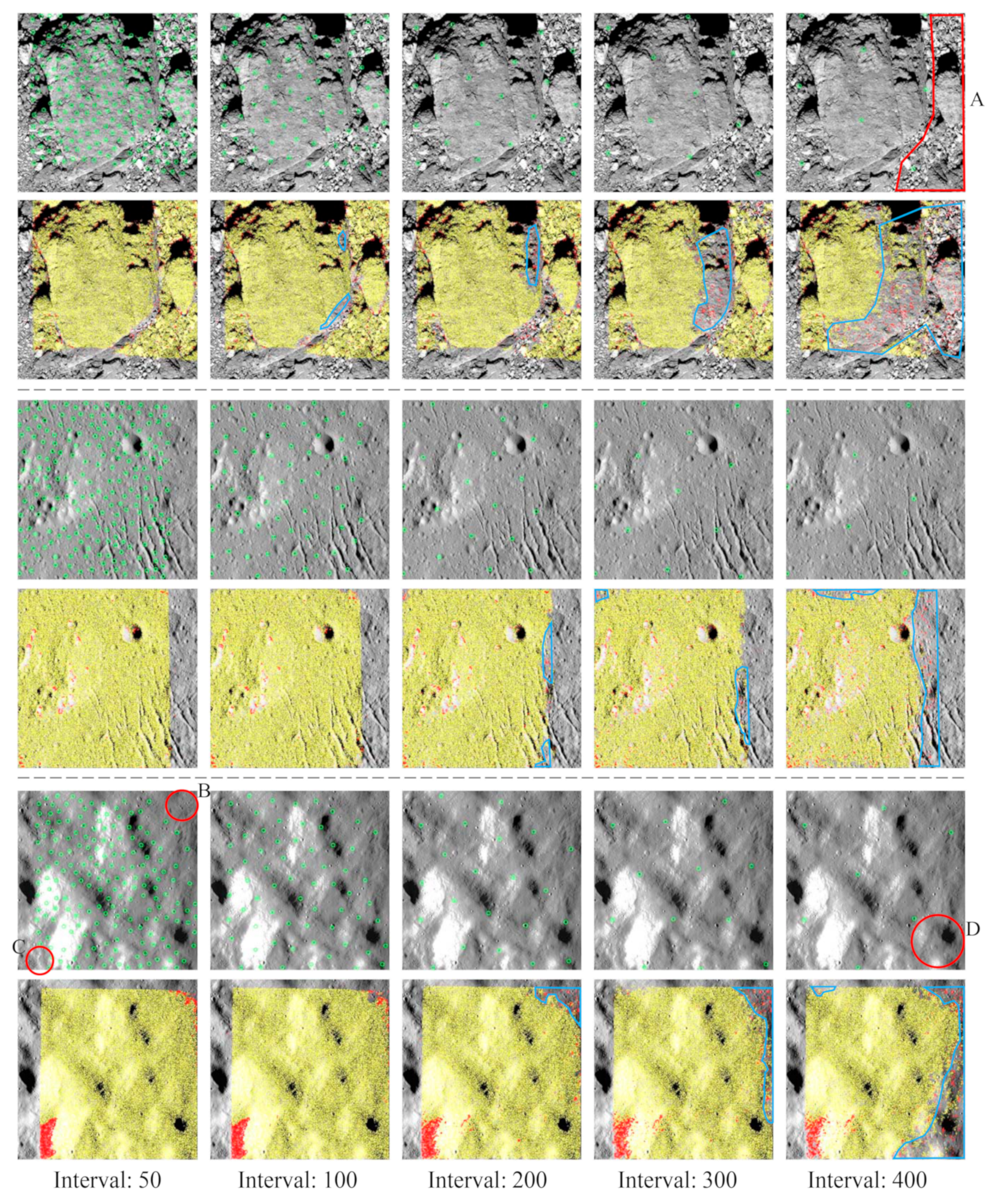
3.3.1. Analysis of Reliable Matching Points on Accuracy

When constructing interim images based on scalar field grids, the distribution and density of reliable matching points affect the results of optical-flow tracking, and we analyze the problem in this section. From Figure 9, the optical-flow fields of Scenes 1, 5, and 6 are more complicated compared to other scenes. Among them, Scene 1 is caused by large terrain changes, and Scenes 5 and 6 are caused by uneven scale changes. We chose these three scenes for detailed analysis.
The experiments in this section are analyzed by setting different intervals between reliably matched points. The distance between points is set to 50, 100, 200, 300, and 400 pixels. The number of homonymous points, the correctness (MA), and the precision (RMS) are used as comparison metrics. The experimental results are shown in Table 4 and Figure 10. From Table 4, the number of homonymous points obtained based on this paper’s method shows an obvious decreasing trend as the interval of reliable matching points increases, and the MA also shows a decreasing trend. The influence of the interval of reliable matching points on the RMS is not obvious.
The regions marked by the red lines in Figure 10 indicate the area where reliable matching points are sparse, while the blue lines indicate the area where homonymous points are sparse. The density of reliable matching points has a significant impact on the results of homonymous points tracking, as shown in “A”–“D” in Figure 10, where the optical-flow-tracking results in these areas marked by red lines are significantly sparser than in other areas. Therefore, a more dense and uniform distribution of reliable matching points is beneficial for obtaining more dense homonymous points. Based on the experiments in this section, this paper recommends using a spacing of 50 pixels in the algorithm implementation.

3.3.2. Quantitative Analysis of Accuracy

Using Equation (10), we can compare the results of different methods using the same criterion, enabling an objective evaluation of their matching accuracy. However, this approach does not provide a quantitative evaluation of the error in the key-point coordinates of the method proposed in this paper. Table 2 and Figure 6 demonstrate that, aside from the method proposed in this paper, the SIFT method exhibits the best matching accuracy. Consequently, in this study, the results of SIFT matching are utilized as the ground truth for verifying the matching accuracy of the method proposed in this paper. To assess the matching accuracy of the proposed method, based on the coordinates of the key points in the current image obtained from the SIFT-matching results, the method proposed in this paper estimates the coordinates of the key points in the next image. Subsequently, the Root Mean Square Error (RMSE) is calculated using Equation (11).
R M S E = i = 1 N ( x i x i ) 2 + ( y i y i ) 2 N .
In Equation (11), xi and yi represent the horizontal and vertical coordinates of the key-points in the next image estimated by the method proposed in this paper. x′i and y′i stand for the horizontal and vertical coordinates of the key-points in the next image matched by the SIFT method, respectively. If the Euclidean distance between the key-point coordinates obtained by the two methods is greater than one pixel, then it is considered an incorrect result. However, all points with a distance of one pixel or less between the key-point coordinates obtained by the two methods are included in the calculation of the RMSE. Additionally, MA denotes the ratio of the number of key-points with a coordinate distance of one pixel or less to the total number of key-points. Table 5 presents the statistical results of RMSE and MA for all matching points in the six scenarios.
Figure 11 displays a density plot depicting the distribution of Euclidean distances between the key-point coordinates obtained from the two methods, measured in pixels. It is evident from Figure 11 that, for the six pairs of images, the Euclidean distance between the coordinates tracked by the method proposed in this paper and the coordinates matched by SIFT primarily falls within the range of less than 0.4 pixels. The peak of the density plot for all 6 scenarios is consistently below 0.2 pixels.
The method proposed in this paper demonstrates excellent accuracy and robustness, as indicated by the experimental results. It achieves accuracy comparable to SIFT feature matching. Notably, this method outperforms mainstream feature-matching algorithms in terms of matching accuracy and the density of key-points obtained. This method effectively addresses the challenges of optical-flow tracking in asteroid multi-view images, including poor photographic conditions, large-scale variations, significant rotation angles, and substantial displacements. In multi-view image matching of Bennu, Ceres, and Vesta asteroids, the proposed method achieved a remarkable matching accuracy exceeding 98%, along with a matching precision of 0.25 pixels in RMSE, outperforming the SIFT feature-matching approach.

4. Conclusions

To explore the technical advantages of the optical-flow method in asteroid image matching, this paper begins by analyzing the characteristics of multi-view images of asteroids and examining the differences among various scene image pairs. Based on these insights, this paper introduces a novel optical-flow-tracking method guided by scale-invariant feature matching and a displacement scalar field, which accounts for the small motion assumption of the optical-flow-tracking algorithm. We innovatively introduce the displacement scalar field grid into optical-flow tracking. The method provides a continuous initial value for optical-flow tracking through the displacement scalar field grid computed by the Kriging interpolation algorithm, which solves the problem of optical-flow tracking under large displacement, uneven scale variation, and a large rotation angle. In addition, we propose an intermediate image-based optical-flow-tracking strategy, which reduces the difficulty of optical-flow tracking by decomposing the optical-flow-tracking steps. By integrating the technical strengths of image feature matching and the optical-flow algorithm, this method achieves image homonymous point-matching results with precision and density. Experimental results demonstrate that the algorithm presented in this paper achieves excellent matching accuracy and density when dealing with challenging scenarios of multi-view images of asteroids.
The method presented in this paper focuses on addressing the small motion assumption of the optical-flow method. However, it is important to note that the optical-flow method also relies on a strong assumption of gray value invariance. Changes in the gray value of homonymous pixel points between two images can significantly affect the accuracy of tracking results. In this paper, only frame-level gray value unification is performed, and no comprehensive investigation is conducted regarding the impact of uneven illumination. Nonetheless, it is crucial to recognize that poor lighting conditions are a prevalent characteristic of asteroid images. Therefore, in our future research, we will conduct in-depth investigations into the optical-flow-tracking problem arising from uneven illumination.

Author Contributions

Conceptualization, Y.X. and S.Z.; methodology, S.Z.; software, S.Z. and Y.T.; validation, R.Z., W.Y. and S.Z.; formal analysis, X.J.; data curation, X.J.; writing—original draft preparation, S.Z.; writing—review and editing, Y.X. and S.Z.; visualization, C.N. All authors have read and agreed to the published version of the manuscript.

Funding

This work was supported in part by the National Natural Science Foundation of China, grant number 42275147.

Data Availability Statement

Data are contained within the article.

Acknowledgments

The authors thank all data providers for their efforts in making the data available: asteroid images from the National Aeronautics and Space Administration (NASA); NASA Planetary Data System.

Conflicts of Interest

Author Ruishuan Zhu is from Shandong Zhengyuan Aerial Remote Sensing Technology Co., Ltd., but the authors declare no conflict of interest.

References

  1. Arnold, G.E.; Helbert, J.; Kappel, D. Studying the early solar system—Exploration of minor bodies with spaceborne VIS/IR spectrometers: A review and prospects. In Proceedings of the in Annual Conference on Infrared Remote Sensing and Instrumentation XXVI held part of the Annual SPIE Optics + Photonics Meeting, San Diego, CA, USA, 20–22 August 2018. [Google Scholar]
  2. Matheny, J.G. Reducing the risk of human extinction. Risk Anal. 2007, 27, 1335–1344. [Google Scholar] [CrossRef] [PubMed]
  3. Zhang, R.; Huang, J.; He, R.; Gen, Y.; Meng, L. The Development Overview of Asteroid Exploration. J. Deep Space Exploration. 2019, 6, 417–423,455. [Google Scholar]
  4. Xu, Q.; Wang, D.; Xing, S.; Lan, C. Mapping and Characterization Techniques of Asteroid Topography. J. Deep Space Explor. 2016, 3, 356–362. [Google Scholar]
  5. Liu, W.C.; Wu, B. An integrated photogrammetric and photoclinometric approach for illumination-invariant pixel-resolution 3D mapping of the lunar surface. ISPRS J. Photogramm. Remote Sens. 2020, 159, 153–168. [Google Scholar] [CrossRef]
  6. Peng, M.; Di, K.; Liu, Z. Adaptive Markov random field model for dense matching of deep space stereo images. J. Remote Sens. 2013, 8, 1483–1486. [Google Scholar]
  7. Wu, B.; Zhang, Y.; Zhu, Q. A Triangulation-based Hierarchical Image Matching Method for Wide-Baseline Images. Photogramm. Eng. Remote Sens. 2011, 77, 695–708. [Google Scholar] [CrossRef]
  8. Lohse, V.; Heipke, C.; Kirk, R.L. Derivation of planetary topography using multi-image shape-from-shading. Planet. Space Sci. 2006, 54, 661–674. [Google Scholar] [CrossRef]
  9. Lowe, D.G. Distinctive image features from scale-invariant key-points. Int. J. Comput. Vis. 2004, 60, 91–110. [Google Scholar] [CrossRef]
  10. Bay, H.; Ess, A.; Tuytelaars, T.; Van Gool, L. Speeded-Up Robust Features (SURF). Comput. Vis. Image Underst. 2008, 110, 346–359. [Google Scholar] [CrossRef]
  11. Cui, P.; Shao, W.; Cui, H. 3-D Small Body Model Reconstruction and Spacecraft Motion Estimation during Fly-Around. J. Astronaut. 2010, 31, 1381–1389. [Google Scholar]
  12. Ke, Y.; Sukthankar, R. PCA-SIFT: A more distinctive representation for local image descriptors. In Proceedings of the 2004 IEEE Computer Society Conference on Computer Vision and Pattern Recognition, 2004. CVPR 2004, Washington, DC, USA, 27 June 2004; p. II. [Google Scholar]
  13. Lan, C.; Geng, X.; Xu, Q.; Cui, P. 3D Shape Reconstruction for Small Celestial Body Based on Sequence Images. J. Deep Space Explor. 2014, 1, 140–145. [Google Scholar]
  14. Liu, X.; Wu, Y.; Wu, F.; Gu, Y.; Zheng, R.; Liang, X. 3D Asteroid Terrain Model Reconstruction Based on Geometric Method. Aerosp. Control Appl. 2020, 46, 51–59. [Google Scholar]
  15. Baker, S.; Matthews, I. Lucas-kanade 20 years on: A unifying framework. Int. J. Comput. Vision 2004, 56, 221–255. [Google Scholar] [CrossRef]
  16. Rodriguez, M.P.; Nygren, A. Motion Estimation in Cardiac Fluorescence Imaging with Scale-Space Landmarks and Optical Flow: A Comparative Study. IEEE Trans. Biomed. Eng. 2015, 62, 774–782. [Google Scholar] [CrossRef] [PubMed]
  17. Granillo, O.D.M.; Zamudio, Z. Real-time Drone (UAV) trajectory generation and tracking by Optical Flow. In Proceedings of the IEEE International Conference on Mechatronics, Electronics and Automotive Engineering (ICMEAE), Cuernavaca, Mexico, 24–27 November 2018; pp. 38–43. [Google Scholar]
  18. Bakir, N.; Pavlov, V.; Zavjalov, S.; Volvenko, S.; Gumenyuk, A.; Rethmeier, M. Novel metrology to determine the critical strain conditions required for solidification cracking during laser welding of thin sheets. In Proceedings of the 9th International Conference on Beam Technologies and Laser Application (BTLA), Saint Petersburg, Russia, 17–19 September 2018. [Google Scholar]
  19. Debei, S.; Aboudan, A.; Colombatti, G.; Pertile, M. Lutetia surface reconstruction and uncertainty analysis. Planet. Space Sci. 2012, 71, 64–72. [Google Scholar] [CrossRef]
  20. Chen, W.; Sun, T.; Chen, Z.; Ma, G.; Qin, Q. Optical Flow Based Super-resolution of Chang’E-1 CCD Multi-view Images. Geomat. Inf. Sci. Wuhan Univ. 2014, 39, 1103–1108. [Google Scholar]
  21. Weinzaepfel, P.; Revaud, J.; Harchaoui, Z.; Schmid, C. DeepFlow: Large displacement optical flow with deep matching. In Proceedings of the IEEE International Conference on Computer Vision (ICCV), Sydney, Australia, 1–8 December 2013; pp. 1385–1392. [Google Scholar]
  22. Brox, T.; Malik, J. Large Displacement Optical Flow: Descriptor Matching in Variational Motion Estimation. IEEE Trans. Pattern Anal. Mach. Intell. 2011, 33, 500–513. [Google Scholar] [CrossRef]
  23. Liu, B.; Chen, X.; Guo, L. A Feature Points Matching Algorithm Based on Harris-Sift Guides the LK Optical Flow. J. Geomat. Sci. Technol. 2014, 31, 162–166. [Google Scholar]
  24. Wang, J.; Wang, J.; Zhang, J. Non-rigid Medical Image Registration Based on Improved Optical Flow Method and Scale-invariant Feature Transform. J. Electron. Inf. Technol. 2013, 35, 1222–1228. [Google Scholar] [CrossRef]
  25. Wang, G.; Tian, J.; Zhu, W.; Fang, D. Non-Rigid and Large Displacement Optical Flow Based on Descriptor Matching. Trans. Beijing Inst. Technol. 2020, 40, 421–426,440. [Google Scholar]
  26. Lucas, B.D.; Kanade, T. An iterative image registration technique with an application to stereo vision. In Proceedings of the IJCAI’81: 7th international joint conference on Artificial intelligence, Vancouver, BC, Canada, 24–28 August 1981; pp. 674–679. [Google Scholar]
  27. Szeliski, R. Computer Vision: Algorithms and Applications; Springer Nature: Cham, Switzerland, 2010. [Google Scholar]
  28. Fischler, M.A.; Bolles, R.C. Random sample consensus: A paradigm for model fitting with applications to image analysis and automated cartography. Commun. ACM 1981, 24, 381–395. [Google Scholar] [CrossRef]
  29. Xue, T.; Mobahi, H.; Durand, F.; Freeman, W.T. The aperture problem for refractive motion. In Proceedings of the IEEE Conference on Computer Vision and Pattern Recognition, Boston, MA, USA, 7–12 June 2015; pp. 3386–3394. [Google Scholar]
  30. Rosten, E.; Drummond, T. Machine learning for high-speed corner detection. In Proceedings of the Computer Vision–ECCV 2006: 9th European Conference on Computer Vision, Graz, Austria, 7–13 May 2006; Volume 9, pp. 430–443. [Google Scholar]
  31. Rizk, B.; Drouet, D.C.; Golish, D.; DellaGiustina, D.N.; Lauretta, D.S. Origins, Spectral Interpretation, Resource Identification, Security, Regolith Explorer (OSIRIS-REx): OSIRIS-REx Camera Suite (OCAMS) Bundle 11.0, urn:nasa:pds:orex.ocams::11.0. NASA Planet. Data Syst. 2021. [Google Scholar] [CrossRef]
  32. Nathues, A.; Sierks, H.; Gutierrez-Marques, P.; Ripken, J.; Hall, I.; Buettner, I.; Schaefer, M.; Chistensen, U. DAWN FC2 CALIBRATED CERES IMAGES V1.0, DAWN-A-FC2-3-RDR-CERES-IMAGES-V1.0; NASA Planetary Data System. 2016. Available online: https://pds.nasa.gov/ds-view/pds/viewDataset.jsp?dsid=DAWN-A-FC2-3-RDR-CERES-IMAGES-V1.0https://pds.nasa.gov/ds-view/pds/viewDataset.jsp?dsid=DAWN-A-FC2-3-RDR-CERES-IMAGES-V1.0 (accessed on 14 December 2023).
  33. Nathues, A.; Sierks, H.; Gutierrez-Marques, P.; Schroeder, S.; Maue, T.; Buettner, I.; Richards, M.; Chistensen, U.; Keller, U. DAWN FC2 CALIBRATED VESTA IMAGES V1.0, DAWN-A-FC2-3-RDR-VESTA-IMAGES-V1.0; NASA Planetary Data System. 2011. Available online: https://pds.nasa.gov/ds-view/pds/viewDataset.jsp?dsid=DAWN-A-FC2-3-RDR-VESTA-IMAGES-V1.0 (accessed on 14 December 2023).
  34. Alcantarilla, P.F.; Solutions, T. Fast explicit diffusion for accelerated features in nonlinear scale spaces. IEEE Trans. Patt. Anal. Mach. Intell 2011, 34, 1281–1298. [Google Scholar]
  35. Leutenegger, S.; Chli, M.; Siegwart, R.Y. BRISK: Binary robust invariant scalable key-points. In Proceedings of the 2011 International conference on computer vision, Barcelona, Spain, 6–13 November 2011; pp. 2548–2555. [Google Scholar]
  36. Pock, T.; Urschler, M.; Zach, C.; Beichel, R.; Bischof, H. A duality based algorithm for TV-L1-Optical-Flow image registration. In Proceedings of the 10th International Conference on Medical Image Computing and Computer-Assisted Intervention (MICCAI 2007), Brisbane, Australia, 29 October–2 November 2007; p. 511. [Google Scholar]
  37. Kroeger, T.; Timofte, R.; Dai, D.X.; Van Gool, L. Fast Optical Flow Using Dense Inverse Search. In Proceedings of the 14th European Conference on Computer Vision (ECCV), Amsterdam, The Netherlands, 11–14 October 2016; pp. 471–488. [Google Scholar]
  38. Bouguet, J.Y. Pyramidal implementation of the affine lucas kanade feature tracker description of the algorithm. Intel Corp. 2001, 5, 4. [Google Scholar]
  39. Hu, Y.L.; Song, R.; Li, Y.S. Efficient Coarse-to-Fine PatchMatch for Large Displacement Optical Flow. In Proceedings of the in 2016 IEEE Conference on Computer Vision and Pattern Recognition (CVPR), Seattle, WA, USA, 27–30 June 2016; pp. 5704–5712. [Google Scholar]
Figure 1. Schematic of the improved optical-flow-tracking algorithm’s framework. Numbers in the scalar field grid-x/y are in pixels. The interim image is a warping of the “next image”. The red lines represent the optical-flow-tracking results of the intermediate steps and the blue lines represent the final optical-flow-tracking results.
Remotesensing 15 05786 g001
Figure 3. Optical-flow-tracking algorithm flowchart.
Remotesensing 15 05786 g003
Figure 5. Schematic diagram of the error matching-point elimination method based on epipolar geometry. C1 and C2 are the positions of Camera 1 and Camera 2, respectively. P is a point in three-dimensional space. p1 and p2 are the mappings of point P on the image planes of Camera 1 and Camera 2, respectively.
Remotesensing 15 05786 g005
Figure 6. Statistics of distribution of epipolar distances by different methods. The distances are in pixels.
Remotesensing 15 05786 g006
Figure 7. Example of different situations of mismatching. The yellow points represent correct matches, while the red points represent incorrect matches.
Remotesensing 15 05786 g007
Figure 8. Optical-flow-tracking results of different algorithms. The seven columns from left to right represent the results of algorithms TV-L1, DeepFlow, DIS, LDOP, PyrLK, CPM, and ours, respectively.
Remotesensing 15 05786 g008
Figure 9. Schematic diagram of the optical-flow field of six experimental scenes. The optical-flow field is represented by the yellow arrow. (af) represent Scenes 1–6, respectively.
Remotesensing 15 05786 g009
Figure 10. The influence of reliable matching point distribution on optical-flow tracking. The top two rows of images are the results of Scene 1, the middle two rows of images are the results of Scene 5, and the bottom two rows of images are the results of Scene 6. The green circles in the images represent reliable matching points.
Remotesensing 15 05786 g010
Figure 11. The method in this paper tracks the error distribution of SIFT key-points.
Remotesensing 15 05786 g011
Table 1. Experimental data.
SceneScene 1Scene 2Scene 3Scene 4Scene 5Scene 6
Current
image
Remotesensing 15 05786 i001Remotesensing 15 05786 i002Remotesensing 15 05786 i003Remotesensing 15 05786 i004Remotesensing 15 05786 i005Remotesensing 15 05786 i006
Next
image
Remotesensing 15 05786 i007Remotesensing 15 05786 i008Remotesensing 15 05786 i009Remotesensing 15 05786 i010Remotesensing 15 05786 i011Remotesensing 15 05786 i012
AsteroidBennuBennuBennuBennuVestaCeres
CharacteristicsLarge terrain changesLarge displacementRotate + Large displacementRotate + Large displacementUneven displacementUneven displacement
Table 3. The comparison results’ statistics of optical-flow algorithms. “Key-points” represent the number of feature points to be tracked. Numbers in bold text format are the best results among all methods.
SceneKey-PointsMethod≤1>1MARMSSceneKey-PointsMethod≤1>1MARMS
Scene
1
8007TV-L108007 Scene
4
4499TV-L104499
DeepFlow08007 DeepFlow04499
DIS3191481639.9%0.54DIS04499
LDOP1271673615.9%0.57LDOP04499
PyrLK727648193.8%0.24PyrLK1956243344.6%0.25
CPM779920897.4%0.42CPM435914096.9%0.42
Ours75195799.2%0.25Ours42495498.7%0.23
Scene
2
5927TV-L105927 Scene
5
1894TV-L1218920.1%0.48
DeepFlow05927 DeepFlow518890.3%0.52
DIS13257952.2%0.58DIS3018641.6%0.58
LDOP05927 LDOP3218621.7%0.55
PyrLK1426274334.2%0.21PyrLK126528781.5%0.40
CPM579713097.8%0.41CPM18088695.5%0.42
Ours56781399.8%0.22Ours17202798.5%0.28
Scene
3
11041TV-L1011,041 Scene
6
4028TV-L11640120.4%0.53
DeepFlow011,041 DeepFlow1840100.4%0.53
DIS6844419762.0%0.45DIS1740110.4%0.48
LDOP6307473457.1%0.47LDOP1740110.4%0.52
PyrLK10,7232299.8%0.17PyrLK931350.3%0.53
CPM10,87816398.5%0.41CPM372530392.5%0.45
Ours10,7671399.9%0.17Ours3870999.8%0.26
Table 4. Statistics of optical-flow-tracking results under reliable matching points at different intervals. “Interval” represents the average distance between reliable matching points. The distances are in pixels.
SceneInterval≤1>1MARMS
Scene
1
5048,678106497.9%0.26
10047,426112997.7%0.26
20043,933117197.4%0.25
30039,574136096.7%0.25
40026,060179093.6%0.25
Scene
5
5059,793132897.8%0.32
10059,919134197.8%0.32
20058,878164697.3%0.32
30056,676163497.2%0.33
40050,724163996.9%0.33
Scene
6
5056,08341599.3%0.25
10055,52444599.2%0.26
20052,02864198.8%0.28
30050,94283698.4%0.31
40041,341125897.0%0.32
Table 5. Method proposed in this paper tracks SIFT key-point results.
SceneScene 1Scene 2Scene 3Scene 4Scene 5Scene 6ALL
MA99.06%99.56%100%98.44%99.99%100%99.51%
RMSE0.230.270.180.370.220.260.25
Disclaimer/Publisher’s Note: The statements, opinions and data contained in all publications are solely those of the individual author(s) and contributor(s) and not of MDPI and/or the editor(s). MDPI and/or the editor(s) disclaim responsibility for any injury to people or property resulting from any ideas, methods, instructions or products referred to in the content.

