Article

Integrating GRACE/GRACE Follow-On and Wells Data to Detect Groundwater Storage Recovery at a Small-Scale in Beijing Using Deep Learning

1
College of Marine Science and Technology, Hubei Key Laboratory of Marine Geological Resources, Key Laboratory of Geological Survey and Evaluation of Ministry of Education, China University of Geosciences, Wuhan 430074, China
2
Beijing Water Science and Technology Institute, Beijing 100048, China
3
Satellite Application Center for Ecology and Environment, Ministry of Ecology and Environment, Beijing 100094, China
4
Department of Civil and Environmental Engineering, National University of Singapore, Singapore 117576, Singapore
5
Institute of Geodesy and Geoinformation, University of Bonn, 53115 Bonn, Germany
6
School of Geodesy and Geomatics, Wuhan University, Wuhan 430079, China
*
Author to whom correspondence should be addressed.
Remote Sens. 2023, 15(24), 5692; https://doi.org/10.3390/rs15245692
Submission received: 19 September 2023 / Revised: 29 November 2023 / Accepted: 4 December 2023 / Published: 11 December 2023

Abstract

:
Groundwater depletion is adversely affecting Beijing’s ecology and environment. However, the effective execution of the South-to-North Water Diversion Project’s middle route (SNDWP-MR) is anticipated to mitigate Beijing’s groundwater depletion. Here, we propose a robust hybrid statistical downscaling method aimed at enhancing the capability of the Gravity Recovery and Climate Experiment (GRACE) to detect the small-scale groundwater storage anomaly (GWSA) in Beijing. We used three deep learning (DL) methods to reconstruct the 0.5° × 0.5° terrestrial water storage anomaly (TWSA) between 2004 and 2021. Moreover, multiple processing strategies were used to downscale the GWSA to 0.25° from 2004 to 2021 by integrating wells and GRACE/GRACE follow-on data from the optimal DL model. Additionally, we analyzed the spatiotemporal evolution trends of GW in Beijing before and after the implementation of the SNDWP-MR. The results show that the long short-term memory model delivers optimal performance in the TWSA reconstruction of Beijing, with the correlation coefficient (CC), Nash–Sutcliffe coefficient (NSE), and root mean square error (RMSE) being 0.98, 0.96, and 10.19 mm, respectively. The GWSA before and after downscaling is basically consistent with wells data, but the CC and RMSE of downscaling the GWSA from 2004 to 2021 are improving by 34% and 31%, respectively. Before the SNDWP-MR (2004–2014), the trend of GWSA in Beijing was 17.68 ± 4.46 mm/y, with a human contribution of 69.30%. After SNDWP-MR (2015–2021), GWSA gradually increased by 10.00 mm per year, with the SNDWP-MR accounting for 18.30%. This study delivers a technical innovation reference for dynamically monitoring a small-scale GWSA from GRACE/GRACE-FO data.

1. Introduction

Freshwater resources are crucial controlling factors for natural resources, ecology, and the environment. Groundwater (GW) is a major component of overall freshwater resources, being the main source of agriculture, industrial, and domestic use [1,2,3,4]. Recently, population and economic growth have put pressure on GW, with extraction and consumption continuing to increase. Overexploitation of GW has caused serious hydrological and geological disasters (such as land subsidence, soil salinization, etc.) that threaten the development of major cities worldwide [5,6]. For example, land subsidence in Mexico City has reached up to 30 cm per year [7]. Melbourne, Jakarta, São Paulo, and a number of cities in India are all suffering severe water scarcity [8,9].
Beijing is the capital of China and serves as the country’s economic, political, and cultural center. It is located on the northwestern margin of the North China Plain (NCP), between longitude 115.7° and 117.4°E and latitude 39.4° and 41.6°N, with an area of approximately 16,410 km2, backed by the Yanshan Mountains and adjacent to Tianjin City and Hebei Province (Figure 1). Beijing plays a crucial role in the Beijing–Tianjin–Hebei urban agglomeration. The western part is mountainous with relatively large topographical fluctuations, while the eastern part is a flat plain [10]. The climate in the region is a typically warm and semi-humid continental monsoon climate, characterized by dry, cold winters and rainy, hot summers. Annual precipitation averages approximately 600 mm, gradually decreasing from east to west. Over the past two decades, accelerated urbanization, dramatic increases in urban water use, intensive agricultural irrigation, and the dry climate have caused severe water scarcity and GW depletion [5].
In 2002, the Chinese government launched the South-to-North Water Diversion Projects (SNDWP), aiming to divert freshwater from the Yangtze River to the north arid regions through three canal pipeline systems: the eastern route of SNDWP (SNDWP-ER), the middle route of SNDWP (SNDWP-MR), and the western middle of SNDWP (SNDWP-WR). The SNDWP-ER is designed to transport water to Hebei Province and the Tianjin Municipality. The SNDWP-WR planned to transport water to the Yellow River in northwest China, but it has not yet started to transport water. The SNDWP-MR was launched in December 2014, aiming to alleviate GW depletion in the NCP, especially for Beijing. By December 2022, it had diverted 58.6 billion m3 of freshwater resources from Danjiangkou Reservoir on the Hanjiang River to the NCP, with around 24% diverted to Beijing. The scheme has been in operation for nearly nine years, so it should be possible to quantify and evaluate its effect on GW in Beijing. It is crucial to obtain long time series and high spatial resolution data for GW in Beijing and to accurately quantify spatial and temporal variations in GW before and after SNDWP-MR. The results will enable further optimization of water resource allocation and management.
Traditional GW monitoring methods suffer from several limitations. They tend to be time-consuming and laborious and are capable only of coarse spatial and temporal resolution. These factors make it difficult to accurately quantify changes in GW [11]. Countries such as the United States and Australia have relatively dense networks of GW monitoring wells, but the specific yields of unconfined aquifers and the storage coefficients of confined aquifers are difficult to determine precisely, leading to inaccurate conversion of water levels from wells into the groundwater storage anomaly (GWSA) expressed as equivalent water height (EWH). Traditional monitoring methods also have other issues, such as high costs, inconsistent data formats, logging errors, and restrictive data-sharing policies between countries and regions worldwide, all of which hinder the effective utilization of measured data for GW studies [12,13].
The successful launch of the Gravity Recovery and Climate Experiment (GRACE) and GRACE follow-on (GRACE-FO) has introduced an innovative and effective approach to global GWSA monitoring [14,15]. GRACE/GRACE-FO have achieved long-term monitoring of the global terrestrial water storage anomaly (TWSA) across the globe from April 2002 to the present with a year of data gaps. Many studies have shown that GRACE/-FO satellites would effectively monitor GWSAs on a large scale [1,8,12,16,17,18,19,20]. For example, Swenson et al. (2003) established a correlation between the accuracy of GRACE-derived GWSA and the sizes of regional study areas. Their findings revealed that the error in GRACE-derived GWSAs remains below 1 cm when the study area exceeds 400,000 km2 [21]. Moreover, the accuracy of the results increases with the expansion of the study area, indicating a positive relationship between study area size and accuracy. Richey et al. (2015) estimated global GWSAs from 2003 to 2013 and confirmed that GW is overexploited in many regions of the world [22]. Famiglietti et al. (2011) filtered and convolved the GRACE spherical harmonic (SH) product to estimate TWSA in the watershed of Central Valley, California, USA [23]. Chao et al. (2018) quantified the GWSA in the Tigris–Euphrates basin by subtracting non-groundwater components from the GRACE TWSA using hydrologic surface model data based on the water balance budget [24]. Yin et al. (2020) assimilated GRACE-derived TWSA into the Community Atmosphere Biosphere Land Exchange model to detect GWSAs in the NCP [25]. However, there were data gaps between GRACE and GRACE-FO, and fragmented data because of GRACE’s battery-powered sensors and coarse spatial resolution limited the hydrological application of the data in small-scale areas.
Two methods are commonly used to fill the GRACE/GRACE-FO data gaps. The first is based on satellite laser ranging (SLR) and satellite data from the European Space Agency’s (ESA) Swarm Earth Explorer mission (Swarm) [26]. However, the spatial resolution of GRACE/GRACE-FO observations does not match the data produced by this method, limiting the accuracy of the fill [27]. The second is a data-driven approach, which has been widely used to reconstruct GRACE-derived TWSA on a local or global scale [27,28,29,30]. In recent years, machine learning (ML) and deep learning (DL) have emerged as prevalent approaches for implementing data-driven methods. ML and DL have facilitated significant advances in satellite-based hydrology. For instance, Mo et al. (2022) employed the Bayesian convolution neural network (BCNN) to reconstruct global GRACE-derived TWSA by integrating meteorological observations and hydrological model data [27]. Uz et al. (2022) reconstructed global GRACE-derived TWSAs using a convolution neural network (CNN), BCNN, and deep convolutional autoencoder [30].
However, the above DL models are more suitable for spatially correlated datasets, such as images. On the other hand, GRACE-derived TWSAs display clear trends, periodicity, and temporal relationships. DL models should effectively capture these time-related signals. Two commonly utilized variants of recurrent neural networks (RNN), long short-term memory (LSTM) [31] and gated recurrent unit (GRU) [32], address the challenges of vanishing and exploding gradients encountered in traditional RNNs. They excel in handling long-term time series data and possess superior gradient propagation and memory capabilities. LSTM and GRU have an explicit structure, resulting in more easily interpreted prediction outcomes. Multi-layer perceptron (MLP) is another widely used model featuring powerful expressiveness through multiple hidden layers [29]. Although it lacks gate structures and memory cells like LSTM and GRU, MLP can be constructed with multiple hidden layers, each comprising numerous neurons, which imparts powerful expressive capabilities [33]. Network parameters are continuously and dynamically optimized through a backpropagation algorithm. To fill the data gaps in GRACE, we developed three DL models, LSTM, GRU, and MLP, to reconstruct GRACE-derived TWSAs in Beijing.
Additionally, there are two common methods for downscaling GRACE/GRACE-FO data: dynamic downscaling and statistical downscaling [34,35,36]. Dynamic downscaling employs regional numerical models with high spatial resolution [25,34], benefiting from incorporating physical mechanisms but requiring complex data from multiple sources and slower calculations [34]. Statistical downscaling is a simpler and more widely applied method which determines the relationship between large-scale factors and small-scale observational data using long-term observational datasets [37]. It is computationally efficient and has been successfully applied by many researchers [20,38,39,40,41,42,43]. For instance, Ning et al. (2014) improved the spatial resolution of GRACE-derived TWSAs using an empirical regression model based on the water balance budget [41]. Seyoum et al. (2019) incorporated measured groundwater levels (GWL) to downscale GRACE-derived GWSAs in Illinois using the machine learning (ML) model, boosted regression tree, demonstrating that the model is capable of accurately reproducing the temporal and spatial changes in GWL anomalies [20]. Ali et al. (2021) downscaled 1° GRACE data (TWSA and GWSA) from the India River Basin to 0.25° using the random forest model (RF) and an artificial neural network (ANN), with the results showing that these two DL models can accurately simulate high-resolution GRACE-derived GWSAs.
Although numerous studies have investigated GWSAs in the NCP [16,17,25,34,44,45,46,47], this research is the first to focus specifically on detecting GWSAs on a small scale in Beijing from downscaled GRACE/GRACE-FO data. The issue is how to incorporate good observations to improve the accuracy and spatial resolution of GRACE-derived GWSAs on such a small scale. This study proposes a robust hybrid statistical downscaling approach to generate high-resolution GRACE-derived GWSAs, which will facilitate the precise assessment of the impact of the SNDWP-MR on GWSA recovery in Beijing. The primary focuses of this study are as follows:
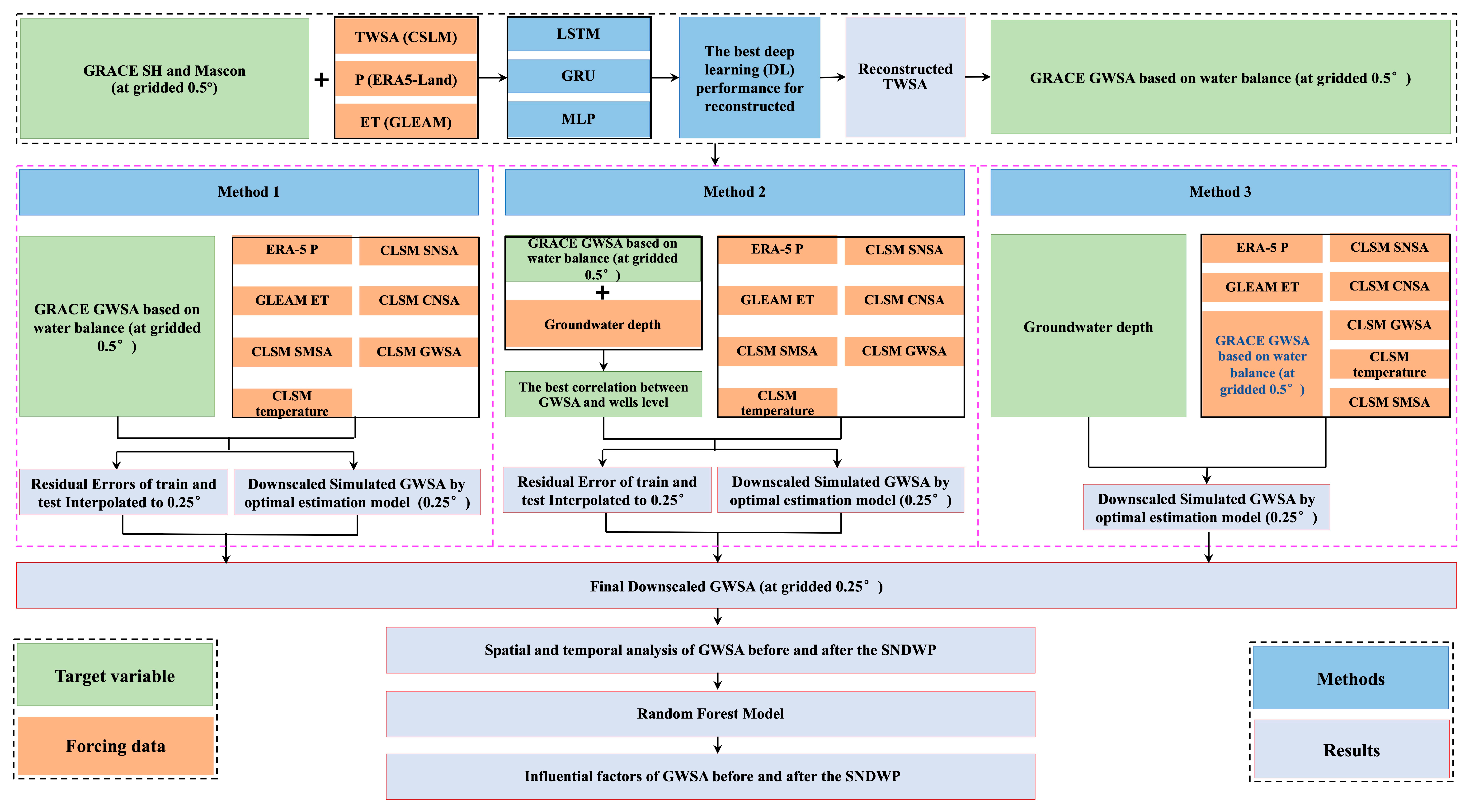
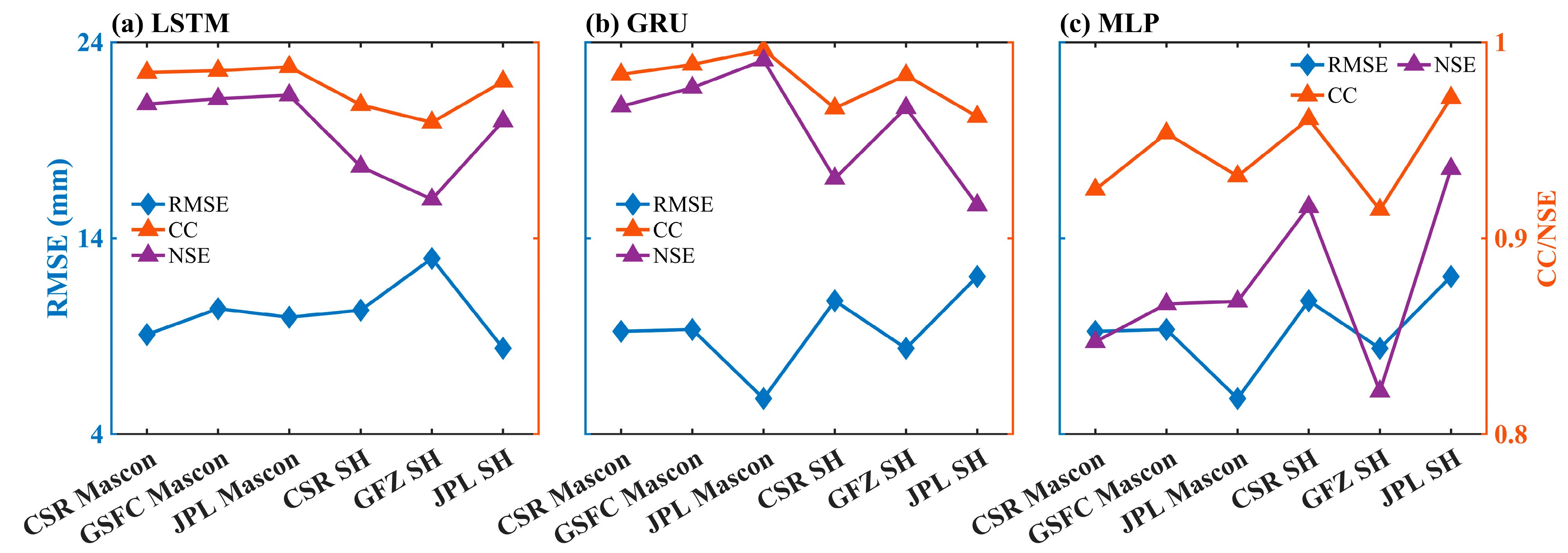
  • Three deep learning (DL) models (LSTM/GRU/MLP) were employed to reconstruct the six types of GRACE-derived TWSAs for the period from January 2004 to December 2021 in Beijing with a spatial resolution of 0.5° × 0.5°.
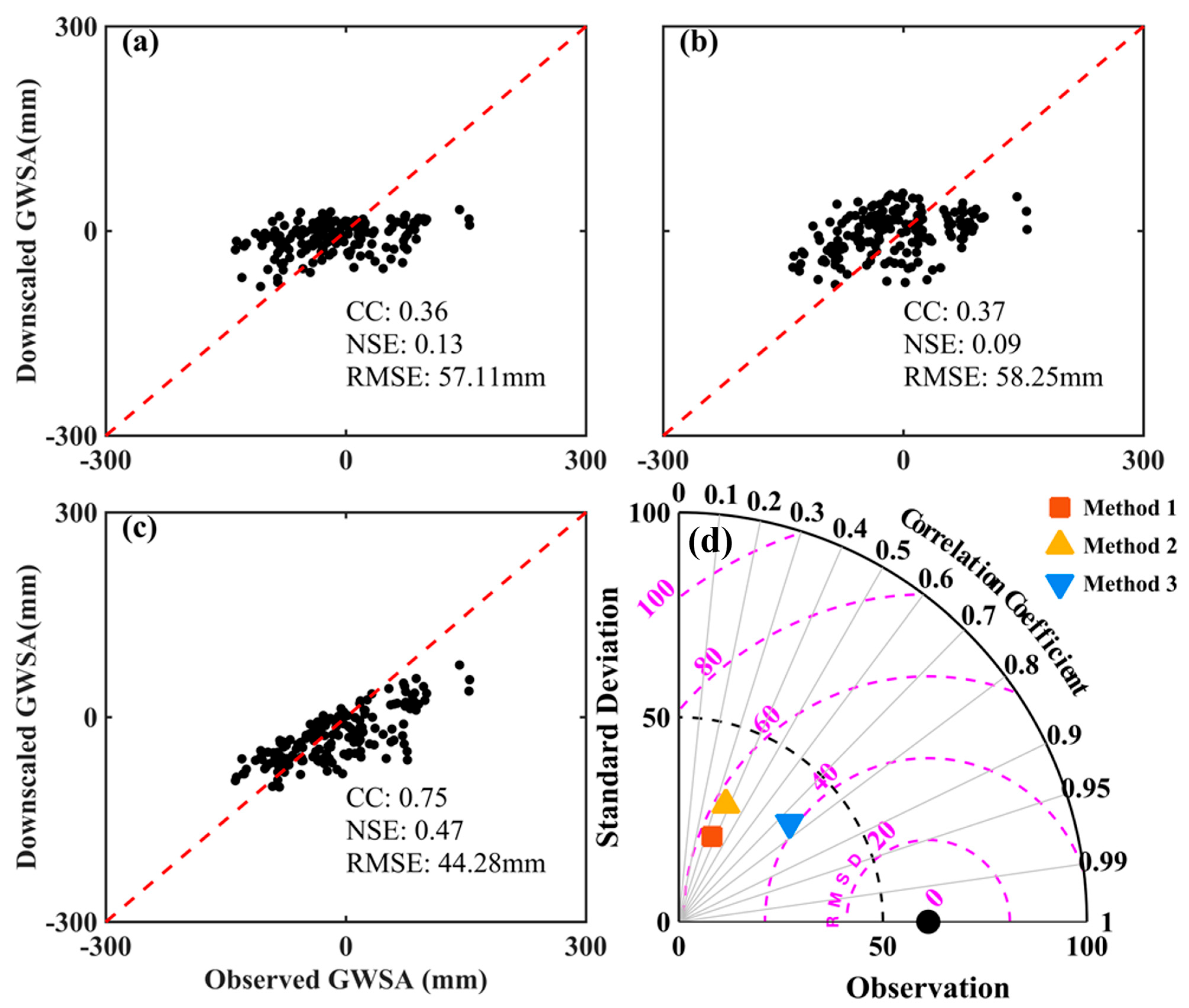
  • Three strategies were explored to incorporate the in-situ data: for Method 1, we treated only the in-situ data as validation data of the downscaled results; for Method 2, we used the in-situ data to identify the downscaling target variables that correlate best with the in-situ data; for Method 3, we used the in-situ data as the downscaling target variable. The optimal DL model, i.e., that with the best performance in step 1, was used to downscale the 0.5° × 0.5° GRACE-derived GWSAs to a higher resolution of 0.25° × 0.25°.
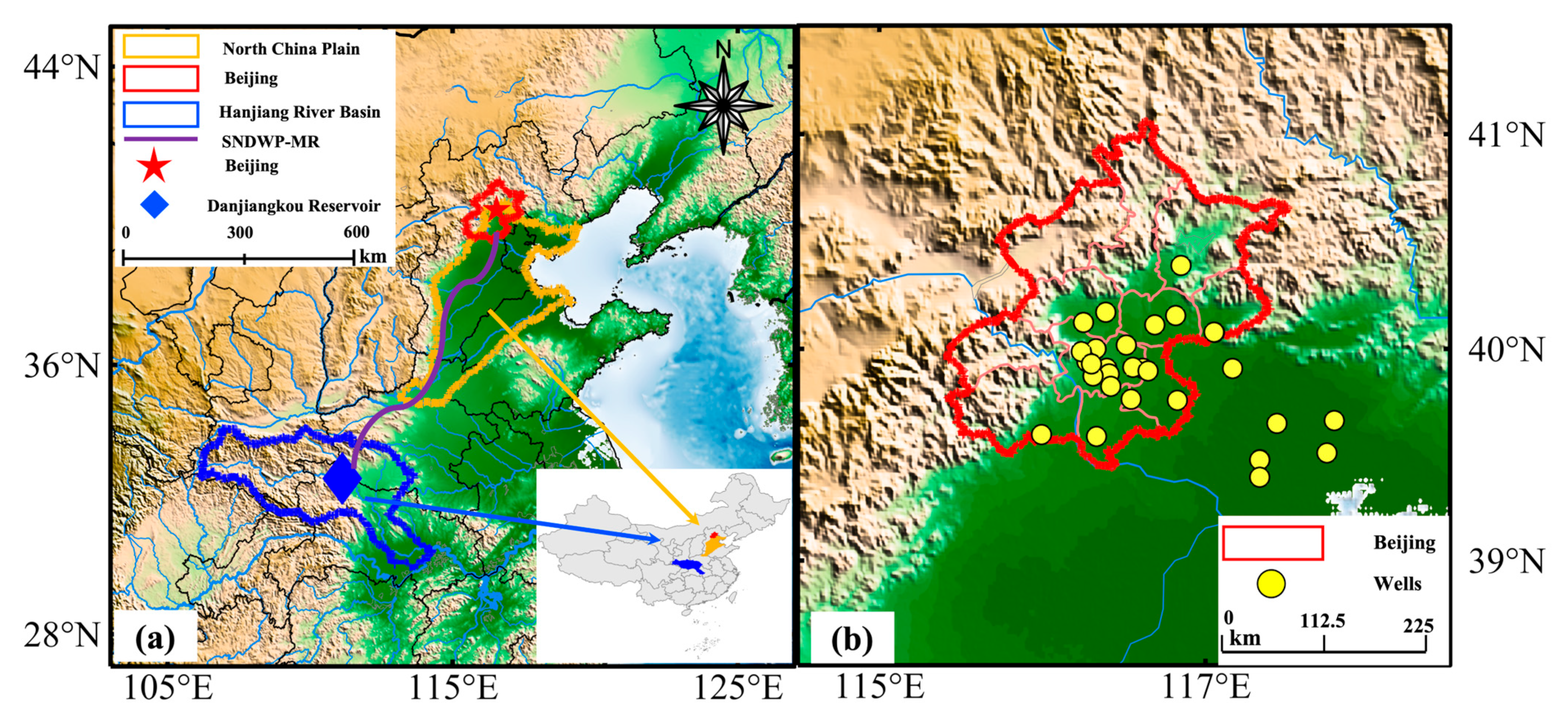
  • The spatiotemporal evolution of GRACE-derived GWSAs in Beijing before and after the implementation of the SNDWP-MR were analyzed and we quantified the contribution of the SNDWP-MR to the spatial evolution of the downscaled GRACE-derived GWSAs using the RF model.

2. Datasets

This study incorporates five distinct datasets: (1) GRACE-derived TWSAs; (2) TWSAs, runoff, surface temperature, soil moisture storage (SMS), snow water equivalent (SNS), and canopy water storage (CNS) provided by the Global Land Data Assimilation System (GLDAS) of the Catchment Land Surface Model (CLSM); (3) precipitation (P) from the ERA5-Land reanalysis product; (4) evaporation (ET) data inferred from the Global Land Evaporation Amsterdam Model (GLEAM); (5) observed data from GW monitoring wells. The temporal resolution of these datasets was standardized to monthly, with spatial resolutions of 0.5° × 0.5° and 0.25° × 0.25°. Table 1 lists the variables used for the reconstruction of GRACE-derived TWSAs, downscaling GRACE-derived GWSAs, and the in situ GWSAs used for validation.

2.1. GRACE-Derived TWSAs

The GRACE/GRACE-FO mass concentration (Mascon) and spherical harmonic (SH) datasets were used from January 2004 to December 2021 provided by the Center for Space Research (CSR) at the University of Texas (https://www2.csr.utexas.edu/grace/RL06_mascons.html) (accessed on 5 October 2023), the Jet Propulsion Laboratory (JPL) (https://grace.jpl.nasa.gov/data/get-data/) (accessed on 5 October 2023), the Goddard Space Flight Center (GSFC) (https://earth.gsfc.nasa.gov/geo/data/grace-mascons) (accessed on 5 October 2023), and the German Research Center for Geoscience (GFZ) (https://www.gfz-potsdam.de/grace) (accessed on 5 October 2023). The Level 2 SH datasets were post-preprocessed to estimate the GRACE-derived TWSA at a 0.25° × 0.25° spatial resolution [48]. The detailed post-preprocessing steps can be found in the Supplementary Information (SI). The GRACE Mascon Level 3 products provide monthly TWSAs (CSR, GSFC, JPL) at a grid resolution of 0.25° × 0.25° or 1° × 1° or 0.5° × 0.5° (Table 1), and their actual spatial resolution is 3° × 3°. However, existing research has demonstrated the effectiveness of the grid resolution of 0.5° × 0.5° [49]. They have already undergone standard corrections, including the C20 and C30 replaced by SRL observations [50], GIA correction by the ICE-6GD (VM5a) model [51,52], ellipsoidal correction, and signal recovery [48,53]. GRACE-derived TWSAs (CSR Mascon, GSFC Mascon, CSR SH, GFZ SH, JPL SH) were resampled to the spatial resolution of 0.5° × 0.5°.

2.2. Precipitation (P)

ERA5-Land monthly reanalysis data, released by the European Weather Forecast Center (ECMWF) (https://cds.climate.copernicus.eu/cdsapp#!/dataset/reanalysis-era5-land-monthly means) (accessed on 5 October 2023), combined modeled data with in situ data from various locations worldwide into a globally comprehensive and consistent dataset. The data are compiled on a monthly scale and cover the period from 1950 to the present. In this study, ERA5-Land reanalysis precipitation was resampled to 0.5° and 0.25° to reconstruct GRACE-derived TWSA and GWSA downscaling.

2.3. Evapotranspiration (ET)

The GLEAM model used inversions of observations from different satellites to obtain the actual evaporation of different terrestrial features [54,55] and it is available for free download at the ESA’s Digital Twin Hydrology project (https://www.gleam.eu/) (accessed on 5 October 2023). In 2017, GLEAM v3 was released, which proposes a new data assimilation scheme optimized for global-scale applications, validated in Australia.

2.4. GLDAS

GLDAS comprises three land surface process models, CLSM, Mosaic LSM, and the Noah land surface model (NOAH), spanning the period from 2003 to the present. It was released by the National Aeronautics and Space Administration’s (NASA’s) Gotha Aeronautics Center (https://ldas.gsfc.nasa.gov/gldas) (accessed on 5 October 2023). The CLSM has the best performance in capturing spatiotemporal variations and long-term trends of TWSA [9,13], so the simulated TWSA, runoff, surface temperature, SMS, SNS, and CNS by the CLSM L4 daily model were used to reconstruct six types of GRACE-derived TWSAs and downscale GRACE-derived GWSAs.

2.5. Well Data

We obtained monthly average GW depths, provided by the Beijing Water Authority (BWA) (https://swj.beijing.gov.cn/) (accessed on 5 July 2023), for each district on the Beijing Plain from January 2007 to December 2021 and yearly average GW depths from 2004 to 2021. Moreover, the monthly GW depths recorded by 41 monitoring wells in Beijing from January 2005 to December 2016 were obtained from the groundwater yearbook published by China Geological Survey Bureau (CGSB) (https://en.cgs.gov.cn/) (accessed on 5 July 2023). The positions of these monitoring wells are depicted in Figure 1b.

3. Methodology

We first used three DL models (LSTM/GRU/MLP) to reconstruct six types of 0.5° × 0.5°GRACE-derived TWSAs (three Mascon products and three SH products) at a regional averaged scale for the period from 2004 to 2021. Then, the optimal DL model, LSTM, was selected to reconstruct the six types of 0.5° × 0.5° GRACE-derived TWSAs mentioned above at a grid scale. Second, we removed non-groundwater components from the six types of 0.5° × 0.5° GRACE-derived TWSAs to obtain the six types of 0.5° × 0.5°GRACE-derived GWSAs. Thirdly, we combined the in-situ groundwater level (GWL) with 0.5° × 0.5° GRACE-derived GWSAs in the optimal DL model, LSTM, and used the three strategies (Method 1, Method 2, and Method 3) outlined to determine the 0.25° × 0.25° GRACE-derived GWSAs in Beijing from 2004 to 2021. Then, we analyzed the spatiotemporal changes in GRACE-derived GWSAs before and after the implementation of the SNDWP-MR. Finally, the contribution of the SNDWP-MR to the GWSA in Beijing was assessed using the random forest (RF) model. The comprehensive methodology flowchart is presented in Figure 2.

3.1. Deep Learning

The core of LSTM is a candidate state and three gates: forget gate, input gate, and output gate. The unique gate structure and memory cells of LSTM provide advantages in controlling information flow and capturing temporal signals such as trends, periodicity, seasonality, and long-term dependencies in temporal data series.
GRU is another RNN model that operates in a similar way to LSTM, utilizing specialized gate structures for information propagation. GRU offers similar advantages to LSTM but has a simpler structure and faster computation, making it well-suited for processing time series data.
MLP is applicable for classification, regression, and unsupervised learning tasks, supporting tasks such as data classification and establishing complex nonlinear mappings [29,33]. The construction of the DL models in this paper was performed using MATLAB 2021(b) [56]. Comprehensive details regarding these three DL models can be found in the supplementary materials.

3.2. Reconstruction of GRACE-Derived TWSAs

In order to fill the data gaps of GRACE-derived TWSAs, this study focuses on three DL models (LSTM/GRU/MLP) using the same external driven input datasets, including 0.5° × 0.5° CLSM TWSA, ERA5-Land P, and GLEAM ET, to reconstruct six types of GRACE-derived TWSAs (CSR Mascon, GSFC Mascon, JPL Mascon, CSR SH, GFZ SH, and JPL SH) in Beijing from 2004 to 2021. Firstly, at the regional scale, we used three DL models (LSTM/GRU/MLP) to reconstruct the six types of GRACE-derived TWSAs (CSR Mascon, GSFC Mascon, JPL Mascon, CSR SH, GFZ SH, and JPL SH). The training period was from January 2004 to December 2015 (~67%), and the testing period covered January 2016 to December 2021 (~33%). Subsequently, we evaluated the permeance of these three DL models and employed the best-performing DL model, LSTM, to reconstruct these six types of GRACE-derived TWSAs at a grid scale. For the reconstruction of GRACE-derived TWSAs at a grid scale, the training dataset consisted of features and targets from 21 grid cells out of 30 grid cells (70%), while the test dataset comprised the remaining 9 grid cells (30%). Therefore, both the training and testing period extended from January 2004 to December 2021.
In this study, the training and testing sets were divided based on grid cells rather than time steps. The reason for this choice is that the research time period (216 months) is relatively short for the DL model, and dividing the data into time periods with shorter time steps can lead to overfitting.

3.3. GWSA in Beijing and Its Downscaled Processing

Due to the lack of vertical resolution in GRACE/GRACE-FO observations, TWSAs determined in this way represent the total water storage anomaly and do not distinguish between surface water, soil water, and groundwater components. In these cases, the GWSA can be determined by subtracting contributions of other hydrological elements from the GRACE-derived TWSA, typically based on the water balance budget [24]:
G W S A = T W S A S M S A S N S A C N S A S W S A ,
where S M S A , S N S A , C N S A , and S W S A are the soil moisture, snow water, canopy water, and surface water storage anomalies, respectively. The TWSA was determined from the six types of GRACE data (CSR Mascon, GSFC Mascon, JPL Mascon, CSR SH, GFZ SH, and JPL SH). The SMSA, SNSA, and CNSA were obtained from the GLDAS CLSM-v2.2. As almost all major rivers in northern China are exploited for municipal and industrial use, they contribute little to TWSA and were therefore ignored [25]. Therefore, the SWSA can be ignored.

3.3.1. Determine GWSA Based on Well Data

Specific yield is described as the volume of water that must be released per unit area of the aquifer for a unit decline in the hydraulic head. Subtracting the mean value from the observation GW depth of monitoring wells (Equation (2)) yields the GWLA, which can be multiplied by the specific yield and converted to equivalent water height (Equation (3)). This study assumed an average specific yield of 0.06 in Beijing [6,16].
G W L A ( t ) = G W L ( t ) G W L ¯ ,
G W S A = 0.06 × G W L A ,
where G W L ( t ) represents the average groundwater level for the month t , and G W L ¯ is the averaged value of GWL for the entire time period.

3.3.2. Downscale of GRACE-Derived GWSA

The downscaled feature variables for Method 1 and Method 2 are ERA5-Land P, GLEAM ET, CLSM SMSA, CLSM SNSA, CLSM CNSA, and CLSM temperature. All the features have two spatial resolutions: 0.5° × 0.5° and 0.25° × 0.25°. The target variables for Method 1 are the six types of GRACE-derived GWSAs (CSR Mascon, GSFC Mascon, JPL SH, CSR SH, GFZ SH, and JPL SH). Additionally, the target variables have only one spatial resolution, which is 0.5° × 0.5°. The target variable for Method 2 was derived from data selection based on the correlation between the six GRACE-derived GWSAs and in situ GWSAs in 14 counties of Beijing. Subsequently, the selected GRACE-derived GWSAs were assembled into a complete grid based on latitude and longitude, which served as the target for Method 2. The features for Method 3 were ERA5-Land P, GLEAM ET, CLSM SMSA, CLSM SNSA, CLSM CNSA, CLSM temperature, JPL Mascon TWSA, and JPL Mascon GWSA’. Except for JPL Mascon GWSA and JPL Mascon GWSA’, the other feature variables have two spatial resolutions: 0.5° × 0.5° and 0.25° × 0.25°. The spatial resolution of JPL Mascon GWSA is 0.5° × 0.5°, and the JPL Mascon GWSA’ is 0.25° × 0.25°. Note that the JPL Mascon GWSA’ was obtained bilinearly interpolated from 0.5° × 0.5° JPL Mascon GWSA and significantly differed from the 0.25° × 0.25° JPL Mascon GWSA after downscaling. The target for Method 3 was the in situ GWSA from 41 wells.
For Method 1 and Method 2, we divided the dataset into training and testing sets based on the number of grid cells. Specifically, 21 grid cells (70%) were used as a training set, while the remaining 9 grid cells (30%) comprised the testing set (Figure S3). We trained the LSTM model using the features and targets with the spatial resolution of 0.5° × 0.5° from the training grid cells and tested the LSTM using features and targets with the spatial resolution of 0.5° × 0.5° from the testing grid cells. Finally, we used the features with the spatial resolution of 0.25° × 0.25° from all grid cells to predict the 0.25° × 0.25° GRACE-derived GWSA ( G W S A D o w n s a c l e S I M ). To reduce the modeling error of the downscale model, we defined the residuals of the training set ( e r r o r T r a i n ) as the differences between the true values of targets from the training set ( G W S A T r a i n T r u t h ) and the LSTM simulated values ( G W S A T r a i n S I M ) (Equation (4)). The residuals of the testing set ( e r r o r T e s t ) are the difference between the true values of the testing set’s target ( G W S A T e s t T r u t h ) and the LSTM simulated values ( G W S A T e s t S I M ) (Equation (4)). Subsequently, e r r o r T r a i n and e r r o r T e s t were interpolated to the 0.25° × 0.25° grids using the Kriging interpolation function (Figure S5), serving as the downscaling model error e r r o r D o w n s c a l e (Equation (5)). Finally, G W S A D o w n s a c l e added to e r r o r D o w n s c a l e to obtain the final downscaled result ( G W S A D o w n s a c l e ) (Equation (6)).
For Method 3, we divided the training and testing sets based on the number of wells. Specifically, 30 wells (~73%) were used as the training set, while the remaining 10 wells comprised the testing set. We trained the LSTM model using features and in situ GWSAs with a spatial resolution of 0.5° × 0.5° from training wells and tested the 0.5° × 0.5° features and in situ GWSAs from testing wells. Finally, we used 0.25° × 0.25° features to predict the 0.25° × 0.25° GRACE-derived GWSA ( G W S A D o w n s a c l e S I M ). Because the 41 wells were concentrated in the southeast corner and could not be interpolated to a complete 0.25° × 0.25° grid, Method 3 did not involve model error estimation. Instead, the model’s predicted value ( G W S A D o w n s a c l e S I M ) was served as the downscaled result (Equation (6)).
e r r o r T r a i n = G W S A T r a i n T r u t h G W S A T r a i n S I M e r r o r T est = G W S A T e s t T r u t h G W S A T e s t S I M ,
e r r o r D o w n s c a l e = K r i g i n g ( e r r o r T r a i n ) ,   the   grid   cell   in   training   set K r i g i n g ( e r r o r T e s t ) ,   the   grid   cell   in   testing   set ,
G W S A D o w n s c a l e = G W S A D o w n s c a l e S I M + e r r o r D o w n s c a l e   Method 1   Method 2 GWSA DownscaleSIM   Method 3 ,
where e r r o r T r a i n and e r r o r T e s t represent the residual error of the training and testing set, respectively. G W S A T r a i n T r u t h and G W S A T e s t T r u t h represent the target variables of the training and testing set, respectively. G W S A T r a i n S I M and G W S A T e s t S I M represent the simulations of the training and testing set, respectively. Kriging is the Kriging interpolation function, e r r o r D o w n s c a l e represents the residual error of downscale, and G W S A D o w n s a c l e represents the GRACE-derived GWSA after downscaling.
In Method 1, the input and target variables are independent of the in situ GWSA. The in situ GWSA was only used for verification of downscaled results. In Method 2, wells data were used to select the GRACE-derived GWSA before downscaling. In Method 3, we integrated the GRACE JPL Mascon GWSA with in situ GWSAs from 41 wells and performed downscaling on the GRACE-derived GWSA. The specific details of these three methods are presented in the SI.

3.4. Random Forest (RF)

In this study, we used the RF model to calculate the contributions of human and climatic factors to the downscaled GRCAE-derived GWSA, with a primary focus on investigating the impact of the SNDWP-MR. The RF model [57,58,59] is a powerful ML model that predicts a feature’s importance by ensembling multiple decision trees. RF model construction in this paper was conducted using SPSS Statistics software (Version 28.0 (R2021)) [60]. The formula for calculating the contributions of the influencing factors using the RF is as follows:
contribution ( j ) = t = 1 T i t r e e t I ( v ( i ) = j ) w i Δ y i 2 t = 1 T i t r e e t w i Δ y i 2 ,
where j represents the factor’s index, t is the decision tree’s index, v ( i ) is the weight of the node i , and Δ y i is the prediction error of the node i .

4. Results

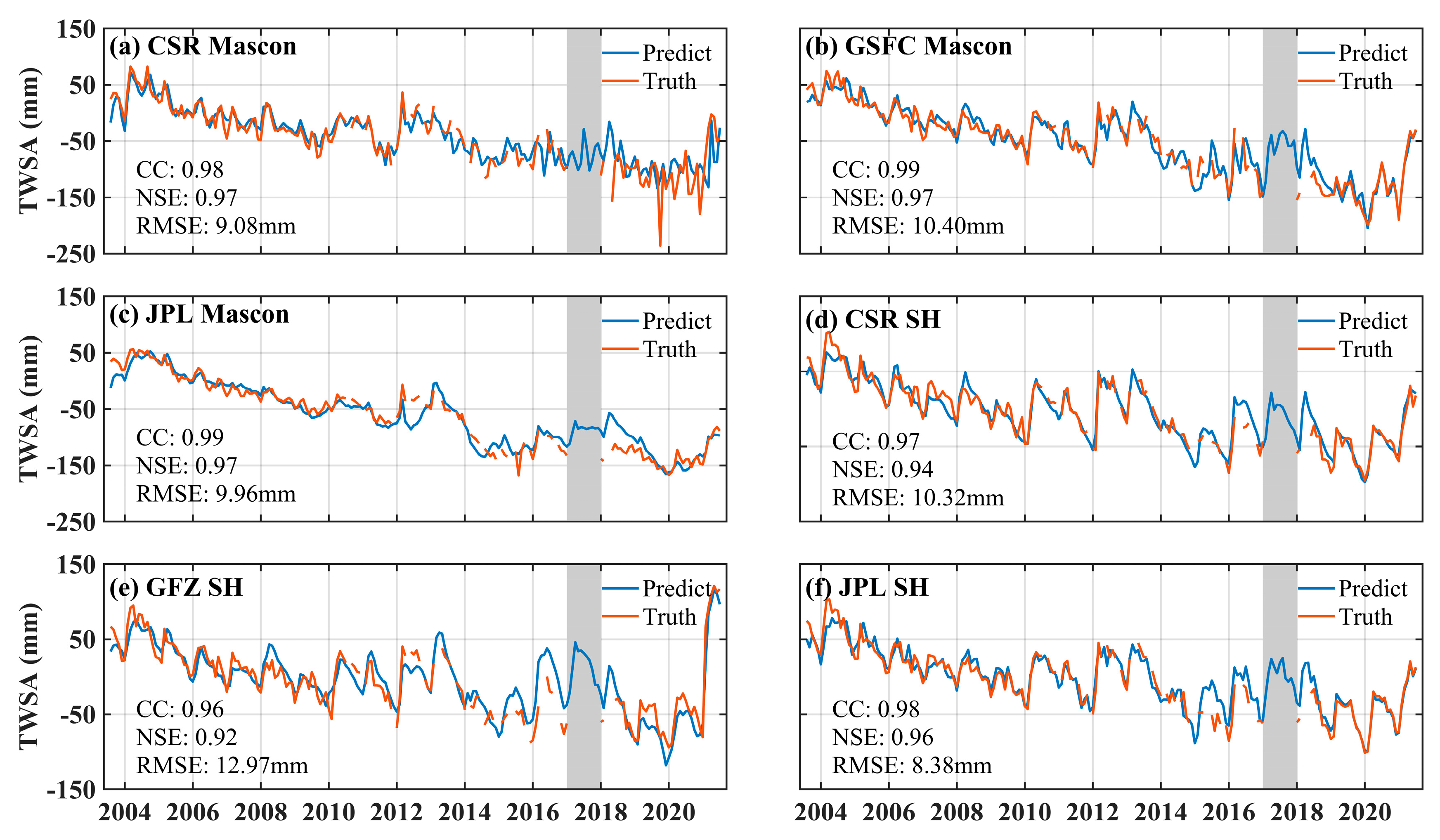
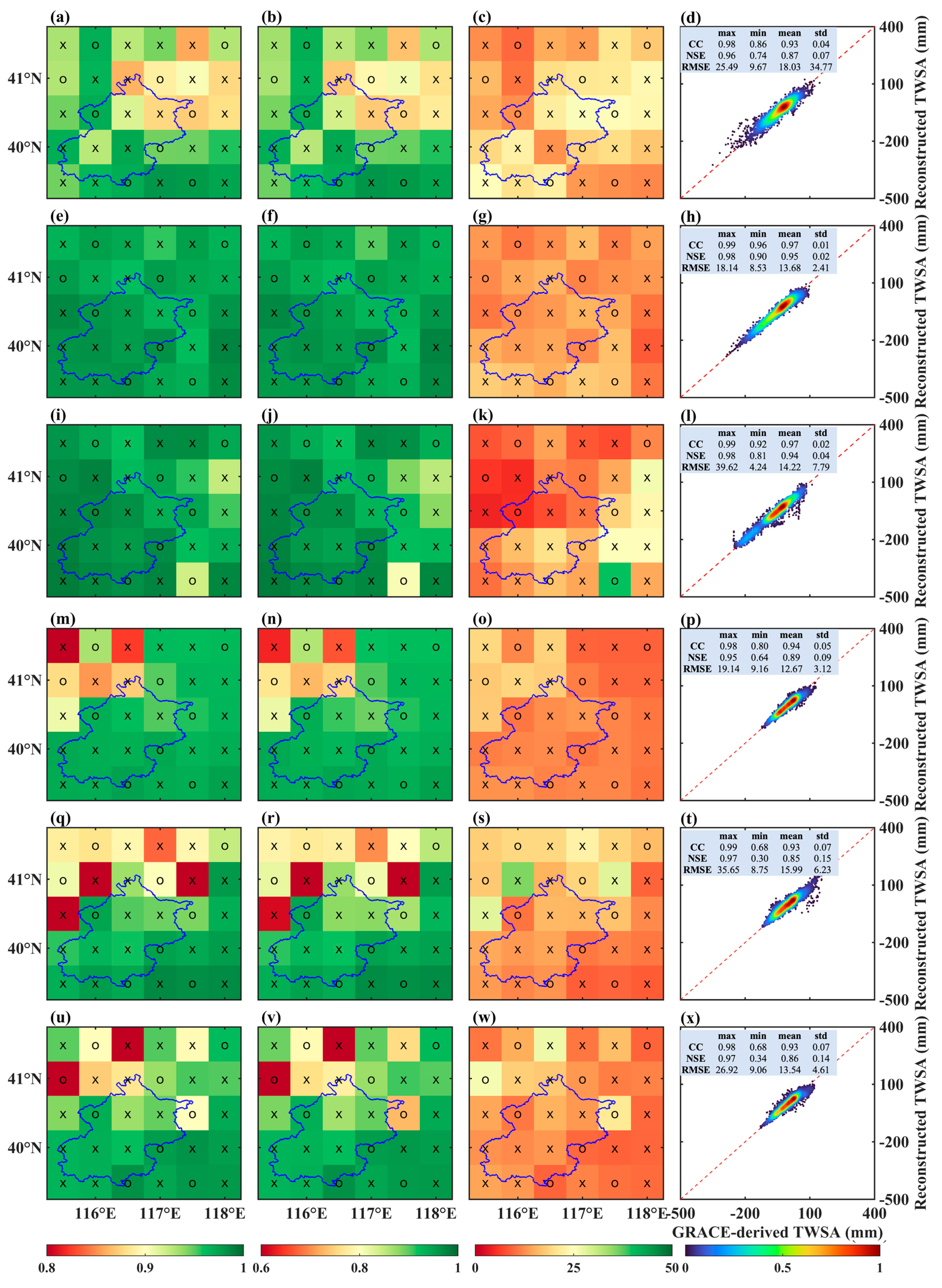
4.1. Reconstruction of GRACE-Dervied TWSAs

Figure 3 represents the correlation coefficient (CC), Nash–Sutcliffe efficiency (NSE), and root mean square error (RMSE) for three DL model-reconstructed GRACE-derived TWSAs compared to the true values of GRACE-derived TWSAs at the regional average scale. Generally, the reconstructed results from all three DL models (LSTM/GRU/MLP) are reasonably accurate, with CCs and NSEs both surpassing 0.8 and RMSEs RMSE ranging from approximately 4 to 24 mm. The MLP demonstrates slightly lower performance, especially on the GFZ SH TWSA, where NSE was 0.82. LSTM and GRU performed similarly, and LSTM slightly outperformed GRU, except for a higher RMSE in GFZ SH TWSA (12.97 mm). The highest accuracy of reconstructing GRACE-derived TWSAs was achieved by the LSTM. In order to save computational resources, the reconstruction of GRACE-derived TWSAs at a grid scale and GRACE-derived GWSA downscaling were used in the LSTM model. Additionally, we will no longer employ GRU and MLP for the reconstruction and downscaling of GRACE data. Therefore, subsequent analysis will focus on LSTM reconstruction results and the downscaling of GWSAs in Beijing using this model.
Table 2 illustrates the CCs, NSEs, and RMSEs for the test and training sets when we used LSTM to reconstruct six types of GRACE-derived TWSAs (CSR Mascon, GSFC Mascon, JPL Mascon, CSR SH, GFZ SH, and JPL SH) at the regional average scale. The training period ranged from January 2004 to December 2015. At the regional scale, the six GRACE-derived TWSAs exhibited strong performance in both the training and testing periods. Specifically, the CSR Mascon TWSA has the highest CC and NSE for both periods, and the RMSE reached 6.16 mm to 14.46 mm. However, the JPL Mascon TWSA showed the lowest NSE for the testing period, only 0.68. We also compared the CC, NSE, and RMSE between the GRACE-derived TWSA reconstructed by LSTM and their truth values during the entire period (2004~2021).
Figure 4a–f shows, on a regional average scale, the six GRACE-derived TWSAs time series and the reconstructed TWSAs time series using LSTM in Beijing from 2004 to 2021 and their error metrics (CC, NSE, and RMSE) in the entire time period. The results show good consistency between the reconstructed GRACE-derived TWSA and their truth value, with CCs and NSEs both exceeding 0.9 and RMSEs ranging from 8 to 13 mm. JPL SH TWSA has the lowest RMSE, indicating the highest reconstruction capability (CC: 0.98, NSE: 0.96, RMSE: 8.38 mm). Conversely, GFZ SH TWSA displays the lowest CC and NSE (CC: 0.96, NSE: 0.92, RMSE: 12.97 mm).
Comparison of GRACE-derived TWSA reconstructed by LSTM with previous research findings [28,30,61] and their truth values reveals the following: the CC between the reconstructed CSR Mascon TWSA and its truth value is 0.98, NSE is 0.97, and RMSE is 9.08 mm. The values reported by Uz et al. (2022) were CC: 0.6, NSE: 0.42, and RMSE: 22.59 mm. Li et al. (2020) reported CC: 0.91, NSE: 0.60, and RMSE: 30.42 mm, an improvement of 6.59%, 61.67%, and 70.15%, respectively. Similarly, for the JPL SH TWSA reconstructed by LSTM, the CC was 0.98, NSE was 0.96, and RMSE was 8.38 mm, whereas Humphrey and Gudmundsson (2019) reported CC: 0.59, NSE: −0.08, and RMSE: 41.41 mm. It is worth noting that they conducted global-scale reconstructions of GRACE-derived TWSAs and exhibited global consistency but significant errors in small-scale regions. In comparison, this study significantly improves on these previous results in reconstructing GRACE-derived TWSAs at small scales using LSTM.
Figure 5 shows the spatial distribution of accuracy between the reconstructed TWSAs using LSTM and their true values as well as the scatter density plots. Where “x” represents the training grids, and “o” represents the testing grids. Figure 5 also displays the maximum, minimum, mean, and standard deviation (std) of CC, NSE, and RMSE. For Mascon products (Figure 5a–l), in summary, the six types of GRACE-derived TWSAs did not exhibit overfitting, with the accuracy of the testing set comparable to the accuracy of the training set. The CCs of three Mascon TWSAs varied from 0.86 to 0.99, with NSEs ranging from 0.74 to 0.98 and RMSEs ranging from 4.29 to 39.62 mm. The scatter plot density fit goodness was also very close to 1. The GSFC Mascon TWSA outperformed the CSR Mascon TWSA and JPL Mascon TWSA and was more stable, with an average CC of 0.97, NSE of 0.95, and RMSE of 13.68 mm. From a spatial perspective in terms of accuracy distribution, the western region showed higher accuracy than the eastern region, while the southern region had higher accuracy than the northern region for Mascon TWSAs. Among the Mascon products, GSFC Mascon TWSA achieved the highest accuracy at the grid scale, with CC exceeding 0.96, NSE exceeding 0.9, and RMSE below 18.14 mm. Conversely, CSR Mascon TWSA displayed the lowest accuracy at the grid scale, with CC, NSE, and RMSE ranging from 0.86 to 0.98, 0.74 to 0.96, and 9.67 to 25.49 mm, respectively. The JPL Mascon TWSA also exhibited lower stability than others, reflecting a std of approximately 7.79 mm. Additionally, the scatter plot density quality for the JPL Mascon TWSA was relatively lower, with some scatter data points showing less concentration. For SH Products (Figure 5m–x), in general, the CCs of three SH TWSAs varied from 0.68 to 0.99, NSEs were between 0.30 and 0.97, and RMSEs ranged from 8.53 to 26.92 mm. The CSR SH TWSA outperformed GFZ SH TWSA and JPL SH TWSA, and the averaged CC was 0.94, NSE was 0.89, and RMSE was 12.67 mm, less stable with a std of 3.12 mm. Additionally, the scatter density fit of the CSR SH TWSA showed the highest goodness of fit, with data points mostly concentrated around the central location. In contrast to the Mascon products, the SH products showed greater accuracy in the eastern region than the western region. CSR SH exhibited slightly higher accuracy than GFZ SH and JPL SH at the grid scale, with CC exceeding 0.80, NSE exceeding 0.64, and RMSE below 19.14 mm, while the CC, NSE, and RMSE of GFZ SH and JPL SH were 0.68~0.99, 0.30~0.97, and 8.53~26.92 mm, respectively.

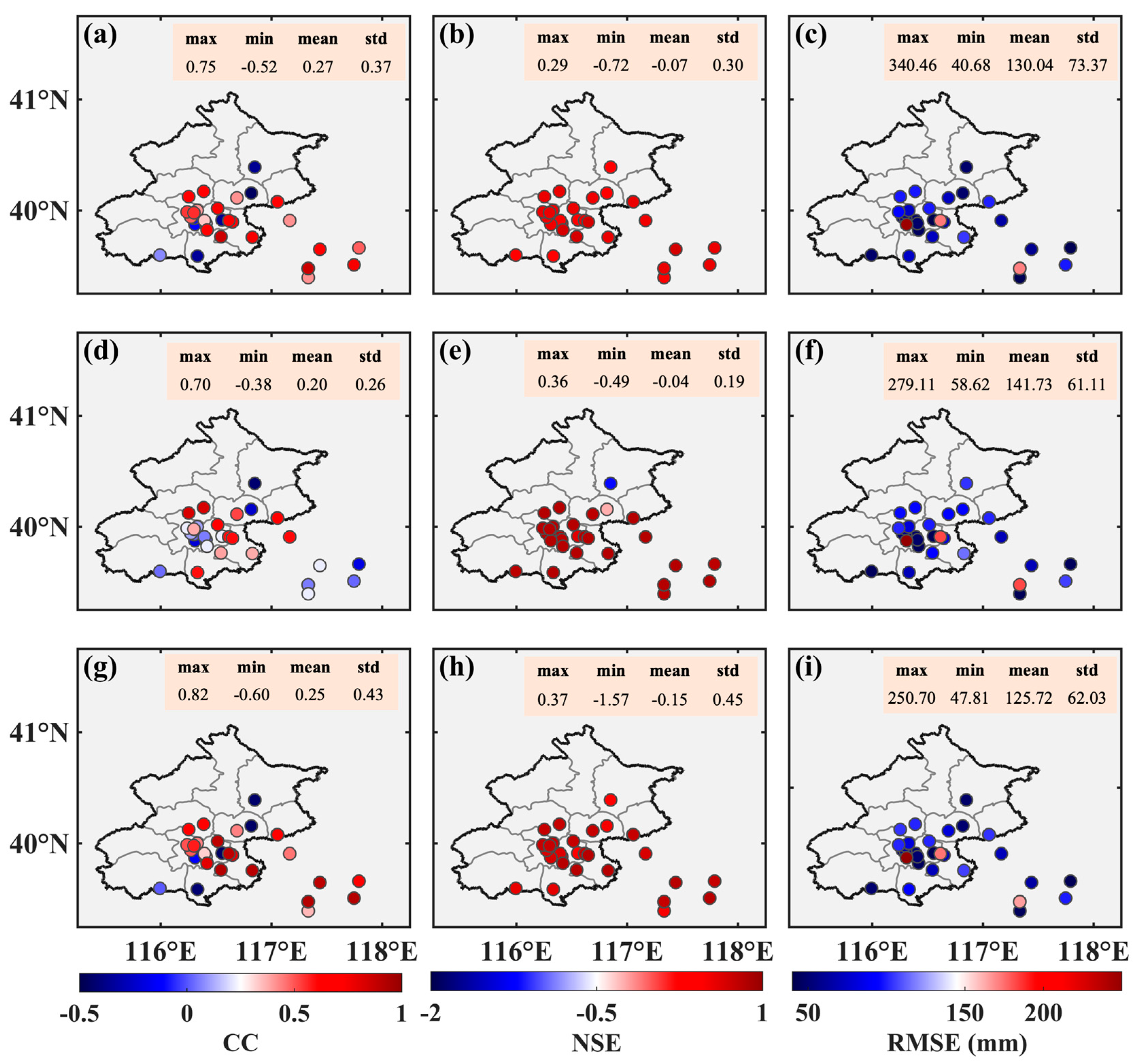
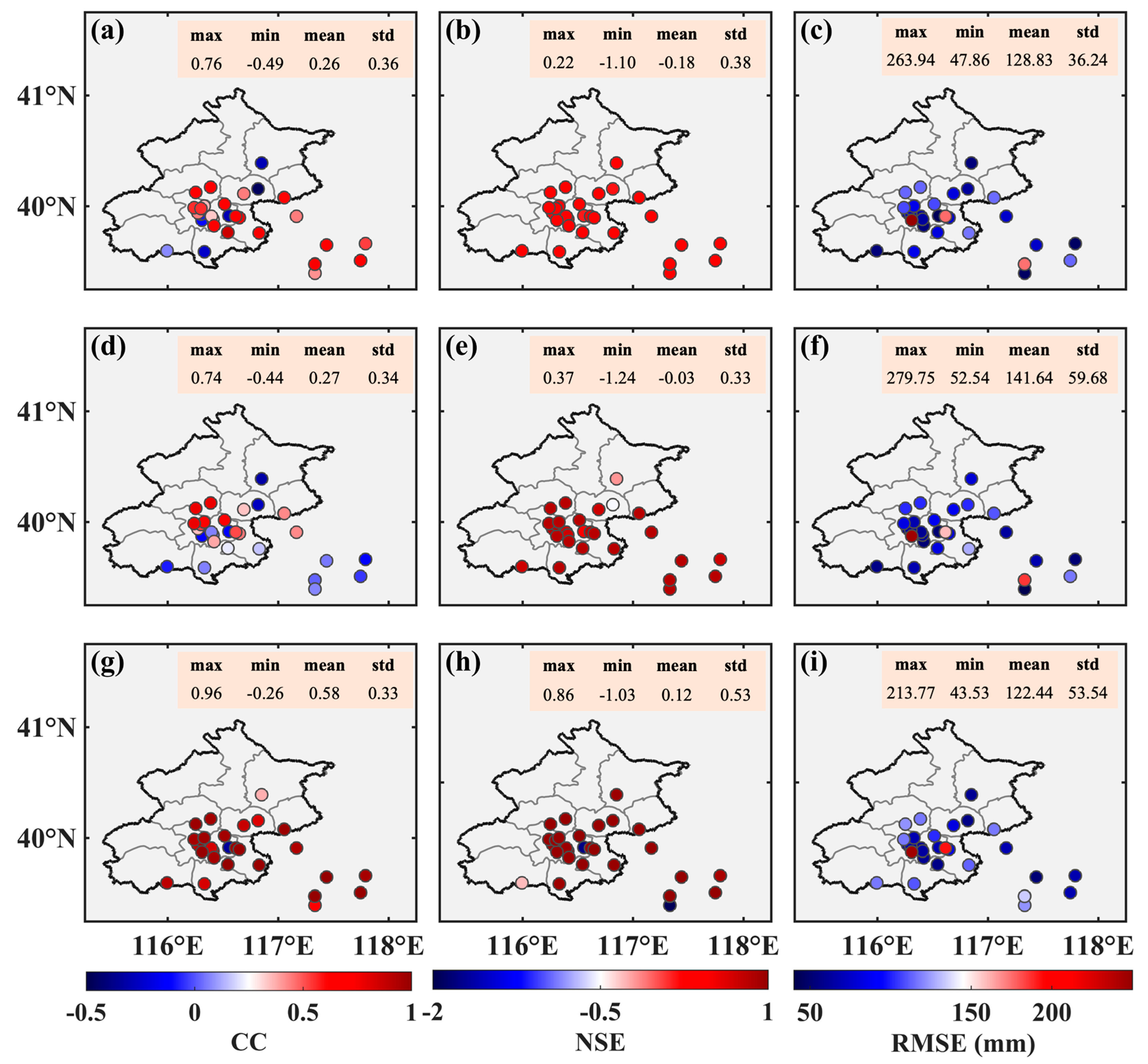
4.2. Downscaling of GRACE-Derived GWSAs

Figure 6 shows the spatial distribution accuracy between the GRACE-derived GWSAs and in situ GWSAs from 41 wells before downscaling and calculates their maximum, minimum, mean, and std. From Figure 6, in general, the accuracies of GRACE-derived GWSAs before downscaling based on the three methods (Method 1, Method 2, and Method 3) are poor, with larger errors compared to in situ GWSAs. Method 2 exhibits the greatest deviation from in situ GWSAs and is less stable, with an average CC of 0.20, NSE of −0.04, and an average RMSE of 141.73 mm. The accuracy of the GRACE-derived GWSA before downscaling using Method 2 is not significantly different from Method 1 when compared to in situ GWSAs. The mean CC of Method 2 is 0.27, the average NSE is −0.07, and the average RMSE is 130.04 mm. Method 3 has a mean CC of 0.25, a mean NSE of −0.15, and an average RMSE of 125.72 mm.
Figure 7 shows the spatial distribution accuracy between the GRACE-derived GWSAs and in situ GWSAs from 41 wells after downscaling and calculates their maximum, minimum, mean, and std. Compared to Figure 6, the differences between the three types of GRACE-derived GWSAs (Method 1, Method 2, and Method 3) and the in situ GWSAs all reduced, with Method 3 (Figure 7g–i) showing the most significant reduction. For Method 3, the averaged CC was 0.58, around twice as much as the value of 0.30 obtained before downscaling. The average NSE was increased from −0.15 to 0.12, and the average RMSE decreased from 125.72 mm to 122.44 mm. For Method 1 (Figure 7a–c), the maximum value of CC was slightly improved and increased from 0.75 to 0.76. Additionally, the average RMSE was 128.83 mm, which improved by 1.57%. For Method 2 (Figure 7d–f), the CC, NSE, and RMSE all improved, with the average CC increasing from 0.20 to 0.27, an improvement of 35.00%. The average RMSE was 134.00 mm, with NSE rising from −0.49 to −0.03 and RMSE reducing from 141.73 mm to 141.64 mm. Additionally, the stabilities of CC, NSE, and RMSE were improved. Therefore, Method 3 is the most effective approach for downscaling GRACE-derived GWSAs. Furthermore, we conducted a statistical analysis of the CC, NSE, and RMSE for both the training and test sets during the downscaling process, as shown in Figure S5 and Tables S1 and S2.
Figure 8 shows the linear fit between the downscaled GRACE-derived GWSAs using three methods (Method 1, Method 2, and Method 3) in situ GWSAs from the Beijing Plain at the regional average scale and a Taylor diagram for accuracy comparison. We used three different colors of symbols to present the three methods (Method 1, Method 2, and Method 3) in the legend of the Taylor diagram. From Figure 8d, it can be seen that the downscaled GWSA based on Method 1 and Method 2, when compared to the in situ GWSA at the regional scale, exhibited similar performance to a std of approximately 25 mm, a centered root square difference (RMSD) of around 60 mm, and a CC of approximately 0.4. The downscaled GRACE-derived GWSA using Method 3 was in the best agreement with the observed GWSA, with an RMSE of 44.28 mm, CC of 0.75, and NSE of 0.47 (Figure 8c). Method 3 performed well at the regional averaged scale, exhibiting the highest CC, NSE, and the lowest RMSE. The downscaling GRACE-derived GWSAs using Method 1 and Method 2 both exhibited relatively low correlations with the in situ GWSA from the Beijing Plain. Method 1 had a CC of 0.36, and Method 2 had a CC of 0.37. Therefore, Method 3 effectively improved the downscale performances of small-scale GRACE-derived GWSAs in Beijing by integrating GRACE data and observed data.
We think there are two main reasons for the low correlation. Firstly, the quality of the in situ GWSA from Beijing Plain was not high. This in situ GWSA was derived from the monthly averaged groundwater depth of 14 counties in Beijing. The detailed steps to process the monthly average groundwater depths from 14 counties into the in situ GWSA of Beijing Plain are outlined in the attachment. Secondly, GRACE-derived GWSAs (CSR Mascon, GSFC Mascon, JPL Mascon, CSR SH, GFZ SH, and JPL SH) before downscaling exhibited a significant discrepancy with the in situ GWSA from the Beijing Plain. The approaches in Method 1 and Method 2 can only enhance the spatial resolution but not improve the correlation at the regional average scale. Method 3, which integrates in situ data from 41 wells, shows some improvement in correlation with the in-situ Beijing Plain.

4.3. Spatial and Temporal Analysis of GWSAs before and after SNDWP-MR

To investigate the contribution of the SNDWP-MR to GW recovery in Beijing, we divided the study period into two stages: Period I (2004.1~2014.12) before SNDWP-MR and Period II (2015.1~2021.12) after SNDWP-MR. We analyzed the trends of downscaled GRACE-derived GWSAs during these two periods at a regional average scale. Figure 9a shows the monthly downscaled GRACE-derived GWSAs using three methods, in situ GWSAs from the Beijing Plain, and P. Additionally, Figure 9b shows the yearly downscaled GARCE-derived GWSAs, in situ GWSA from the Beijing Plain, and P. Overall, the trends of downscaled GRACE-derived GWSAs using three methods demonstrate an agreement with observed data. During Period I, the downscaled GRACE-derived GWSAs both showed a declining trend. In contrast, during Period II, they both showed an increasing trend.
However, there was a time lag of 5~6 months between precipitation and the in situ GWSA. The maximum value of the in situ GWSA occurred around December each year, and the minimum value occurred around June, while precipitation reached its maximum value around June every year. The downscaled GRACE-derived GWSA using Method 3, which incorporates in situ GWSAs, shows a time lag between GWSA and precipitation of approximately 5~6 months, like that of the in situ GWSA. However, the downscaled GRACE-derived GWSAs using Method 1 and Method 2 exhibited a shorter time lag, approximately 3~4 months, between precipitation and the in situ GWSA (Figure S5). The maximum value appeared from September to October, while the minimum value occurred from March to April each year. On a yearly scale, the variations in downscaled GRACE-derived GWSAs were closely related to precipitation. In other words, in years with higher precipitation, GWSAs tend to increase, while in years with lower precipitation, they tend to decrease.
The time lags between precipitation and downscaled GRACE-derived GWSAs based on Methods 1 and 2 were shorter compared to the in situ GWSA. There are two possible explanations for this: (1) replenishment of GW through precipitation requires time, so the measurable response of GW to precipitation is delayed; (2) the study area primarily consists of deep, confined aquifers, which do not respond to GW changes as quickly, or to the same degree, as shallow, unconfined aquifers.
In 2021, the downscaled GRACE-derived GWSAs using three methods deviated slightly from the in situ GWSA, which may be related to the GRACE-derived TWSA and the rapid escalation in precipitation, as it did not detect any signal of a dramatic rise in TWSA in 2021. Although Method 3 incorporates in situ data for downscaled GWSA, the collected in situ data used in this study covered the period from 2005 to 2016 and, therefore, does not reflect any substantial increase in GWSA in 2021. We will discuss the uncertainty of the downscaled GRACE-derived GWSA in Section 5.
Figure 10 depicts the trends of GRACE-derived GWSAs before downscaling during two periods at the grid scale. Overall, the spatial details of GRACE-derived GWSAs before downscaling appear relatively coarse. From a spatial perspective, before the implementation of SNDWP-MR, the GRACE-derived GWSAs both exhibited a declining trend. Moreover, the trends using three methods before downscaling exhibited a more significant decline rate. After the implementation of SNDWP-MR, the GRACE-derived GWSAs generally exhibited an increasing trend. However, there were a few grid cells in the southwestern region that continued to show a declining trend, and these grid cells had the most significant decreasing trend before the implementation of SNDWP-MR (Figure 10a–c). For Method 1 (Figure 10d) and Method 3 (Figure 10f), the trends in the northwest region had a higher rate of increase than the southeastern region. However, for Method 2 (Figure 10e), the trends rose most rapidly along the southeast diagonal. The spatial distributions of trends from these methods (Method 1, Method 2, and Method 3) exhibited some differences, likely attributed to the uncertainties of GRACE-derived GWSAs.
Figure 11 depicts the trends of GRACE-derived GWSAs after downscaling using three methods during two periods at the grid scale. The three downscaled results (Figure 11) present more detailed spatial features than the original GRACE-derived GWSA (Figure 10). Method 1 and Method 2 (Figure 11a,b) (Figure 11d–e) exhibit trends after downscaling that are consistent with the original results (Figure 10a,b) (Figure 10d–e), which indicates that the downscaling approaches based on Method 1 and Method 2, improved the spatial resolution of the GRACE-derived GWSAs. However, the downscaling approach based on Method 3 not only improved the spatial resolution but also altered the spatial distribution of the trends. This is because the downscaling approach of Method 3 incorporated in situ GWSAs from 41 wells. From Figure 11c, it is evident that before SNDWP-MR, the spatial trend of the downscaled GRACE-derived GWSA based on Method 3 reached −50 to 0 mm/y. Before downscaling, the range was −10 to 0 mm/y. Similarly, after SNDWP-MR, the spatial trends of the downscaled GRACE-derived GWSA based on Method 3 (Figure 11f) ranged from 0 to 50 mm/y, whereas before downscaling (Figure 10f), the range was only 0 to 10 mm/y. The reasons for the differences in the spatial distribution of downscaled GRACE-derived GWSA trends among the three methods will be discussed in Section 5.

4.4. The Influence Factors on GWSA

Before SNDWP-MR, there was a shortage of approximately 1 km3/y between water supply and water use, leading to the depletion of GW in Beijing [3]. To further understand the water usage and supply situation in Beijing during the study period, data on different components of the water supply and water allocation were obtained from the Beijing Water Resources Statistics Year Books (Figure 12a).
We utilized the RF to estimate the impacts of human and climatic factors on Beijing’s GWSA. From Figure 12b, it is evident that human factors outweigh climate factors in importance. Before SNDWP-MR, human factors accounted for 69.30%, while climate factors contributed 30.70%. Among the human factors, the contributions of agricultural and industrial water use (the predominant human factors) were 21.40% and 16.10%, respectively; the contribution of SNDWP-ER was only 4.80%. However, water diversion by SNDWP-MR and suppression of agricultural water use caused a significant shift in contribution patterns. After SNDWP-MR, the contribution of human factors decreased to 57.70%, while climate factors increased to 42.30%. Notably, agricultural water usage and SNDWP-MR water volume emerged as the primary human factors, contributing 19.30% and 18.30%, respectively.

5. Discussion

This study employed three DL models to fill the gaps in GRACE-derived TWSAs and utilized a robust hybrid statistical downscaling method to evaluate the application of GRACE for monitoring GWSAs at a small-scale. We also quantified the impact of human and climatic factors on the downscaled GWSA in Beijing before and after the implementation of SNDWP-MR.
We used a generalized three-cornered hat (TCH) to estimate the uncertainty of downscaled GRACE-derived GWSAs [53] (Method 1, Method 2, and Method 3) at a regional average scale. Additionally, the uncertainty of in situ GWSAs was quantified by assuming ±20% uncertainty of the specific yield [17]. The shaded area in Figure 9 represents the uncertainty of GWSA. Whether at a monthly or yearly scale, the uncertainties of downscaled GWSAs and in situ GWSAs are relatively small. At the regional scale, the uncertainty will not have a significant adverse impact on the downscaled GWSA.
In the past, there have been numerous studies of the temporal and spatial evolution of the GWSA in NCP and their cause. Feng et al. (2013) were the first to use GRACE data to estimate the depletion rate, finding a depletion rate of 22.00 ± 3.00 mm/y for the GWSA in the NCP from 2003 to 2013 [1]. Zhang et al. (2021) analyzed the GWL from 617 wells and compared the data with GRACE-derived GWSA [17]. The results showed a GWSA depletion rate of 19.10 ± 5.10 mm/y from 2003 to 2014 and a GW recovery rate of 1.80 ± 0.70 mm per year from 2015 to 2018. Zhao et al. (2019) determined a GW depletion pace of 17.00 ± 1.00 mm/y in the NCP from 2004 to 2016 using GRACE (-FO) data and CLSM [62]. Long et al. (2020) used well observation data to estimate a GWSA depletion rate of 17.50 ± 0.80 mm/y on the Beijing Plain from 2005 to 2014 [5]. In this study, Method 3 estimated a GWSA depletion rate in Beijing of 17.68 ± 4.46 mm/y from 2004 to 2014 and a recovery rate of 10.00 ± 4.77 mm/y from 2015 to 2021, which is basically consistent with the results of previous studies and monitoring well data. The results of Methods 1 and 2 were significantly different from the in-situ observations. During period I, the downscaled GWSA based on Method 1 showed a declining trend at a rate of −4.07 ± 1.60 mm/y and the downscaled GWSA based on Method 2 is −4.39 ± 2.48 mm/y. During period II, the trend of the downscaled GWSA based on Method 1 is 5.04 ± 5.00 mm/y, and the trend of the downscaled GWSA based on Method 2 is 20.25 ± 7.40 mm/y (Table 3).
There are four possible reasons for these significant differences in results between the three methods and in situ data (Figure 11 and Table 3): (1) due to spatial and temporal resolution limitations, the original GRACE observations have a high degree of uncertainty in small-scale areas at grid scale; (2) GW monitoring wells in the eastern plain are mainly deep, confined wells. Studies have shown that from 2015 to 2017, GWLs in shallow, unconfined wells remained stable, while those in deep confined wells decreased rapidly [63]. Hence, the trend of GWSA estimation based on Method 3 is inevitably closer to the measured data; (3) CLSM has limited representativeness for simulating GWSA in the NCP. The simulated GWSA is limited by the soil profile water storage capacity, which is a product of the fixed depth of bedrock and porosity. Döll et al. (2014) suggested that CLSM cannot reproduce the effect of long-term [8], intense GW depletion in large-scale irrigation areas such as the NCP and northern India. Although GW extraction for irrigation has caused a significant decline in GWSA in the NCP, simulating GWSA by CLSM does not reflect this trend [64]; (4) CLSM lacks a dynamic module to simulate surface water and therefore cannot simulate surface water anomalies in Beijing. Thus, separating non-groundwater components from GRACE-derived TWSA vastly reduces the accuracy. However, some studies have indicated the contribution of surface water to TWSA in northern China can be ignored [25].
The downscale approach of Method 3 was used to address the lack of monitoring wells in the study area. Only 41 wells were available, as other observation wells had to be excluded due to data gaps of more than 3.50 years, loss of location information, or failure to distinguish confined and unconfined wells. The monitoring wells were primarily concentrated in the south of the study area. The specific yields were also uneven, and monitoring wells data covered only 2005 to 2016, shorter than the study period (2004~2021). Despite these limitations, a high spatial resolution downscaled GRACE-derived GWSA was obtained based on Method 3 at a small-scale study area. The results for this area are consistent with previous research and show good consistency with the measured data. This suggests that the approach developed in this research provides a new approach to exploring small-scale GRACE-derived GWSAs. Although, in this study, we underestimated the GWSA in Beijing and did not detect the sharp increase in the 2021 GWSA signal, the results will be greatly improved if the period wells data match the study period.

6. Conclusions

This study proposed a robust hybrid statistical downscaling method, which was arrived at by first comparing and analyzing the accuracy of three DL models (LSTM/GRU/MLP) in reconstructing GRACE-derived TWSAs and constructing a long-term TWSAs dataset for Beijing. Subsequently, the best-performing DL model was used in conjunction with three strategies for monitoring well observation data, achieving downscale estimates for 0.25° × 0.25° GRACE-derived GWSAs in Beijing from 2004 to 2021. Finally, the RF model was employed to quantify the contributions of human factors (domestic, industrial, and agricultural water use, etc.) and climate factors (such as P, ET, and runoff) to GRACE-derived GWSAs in Beijing before and after the implementation of SNDWP-MR. The principal findings can be summarized as follows:
  • Six different GRACE-derived TWSA time series were reconstructed for Beijing from 2004 to 2021, with the LSTM model performing the best, followed by GRU with slightly lower performance, and MLP, which performed the worst.
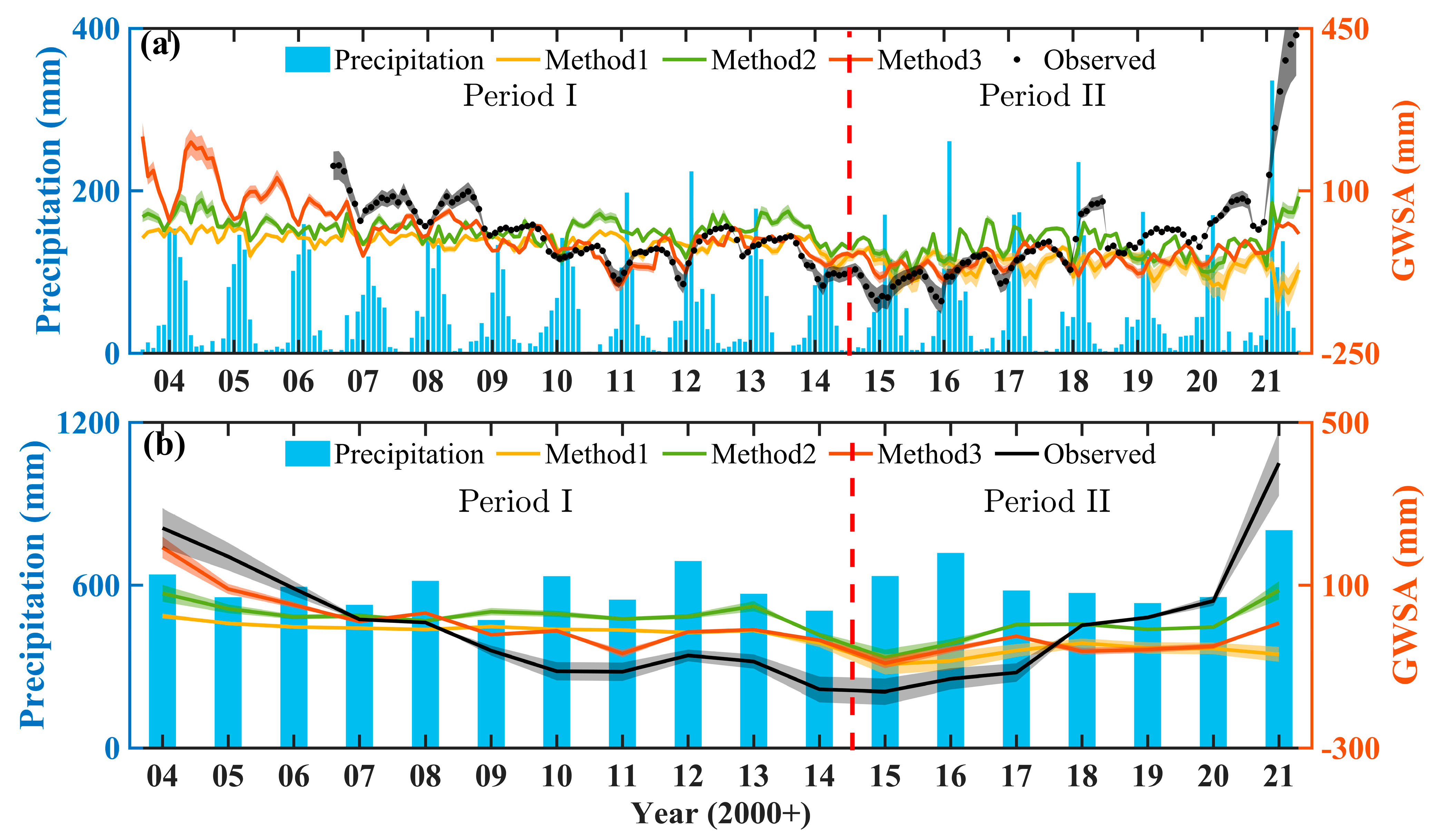
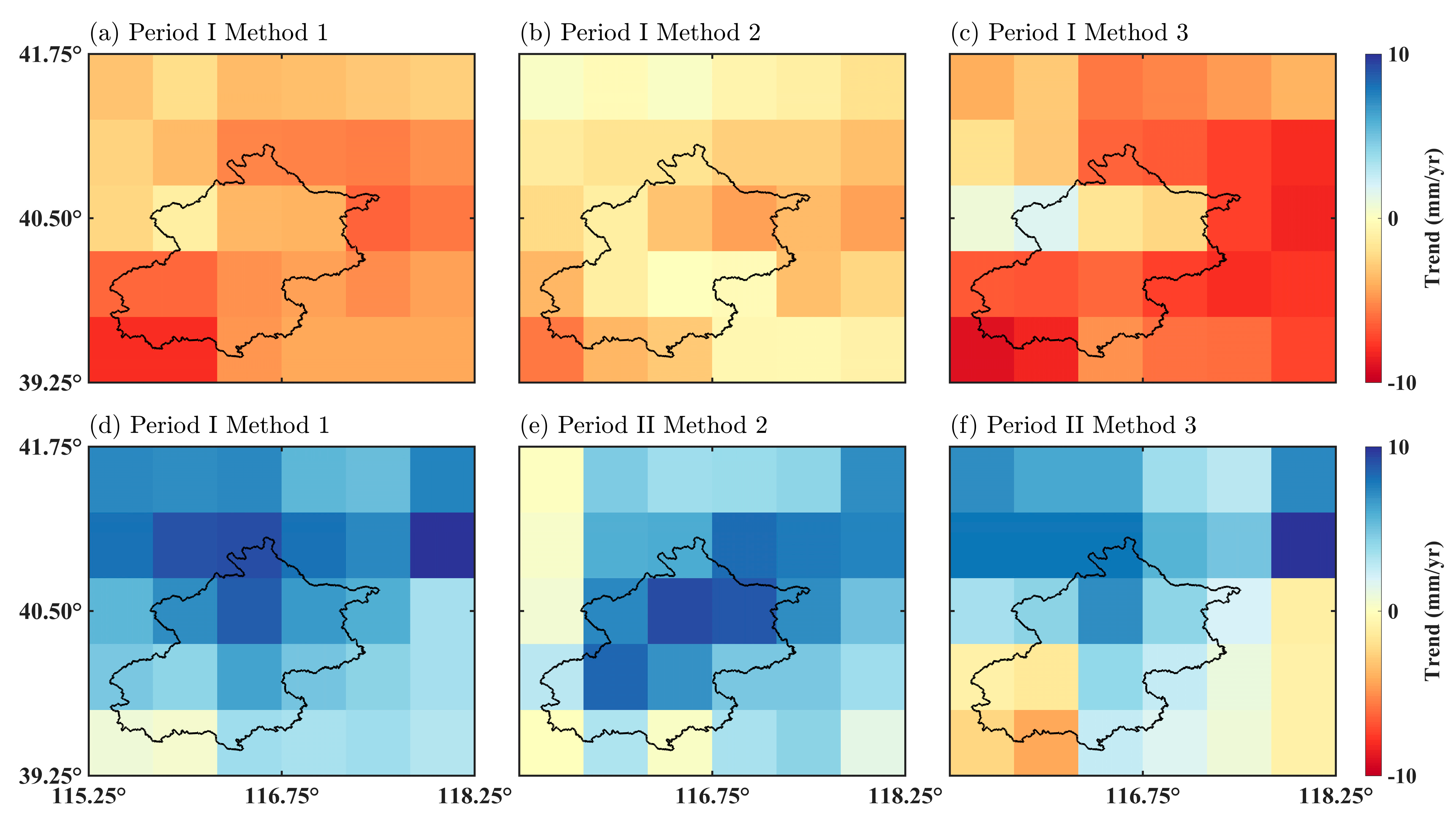
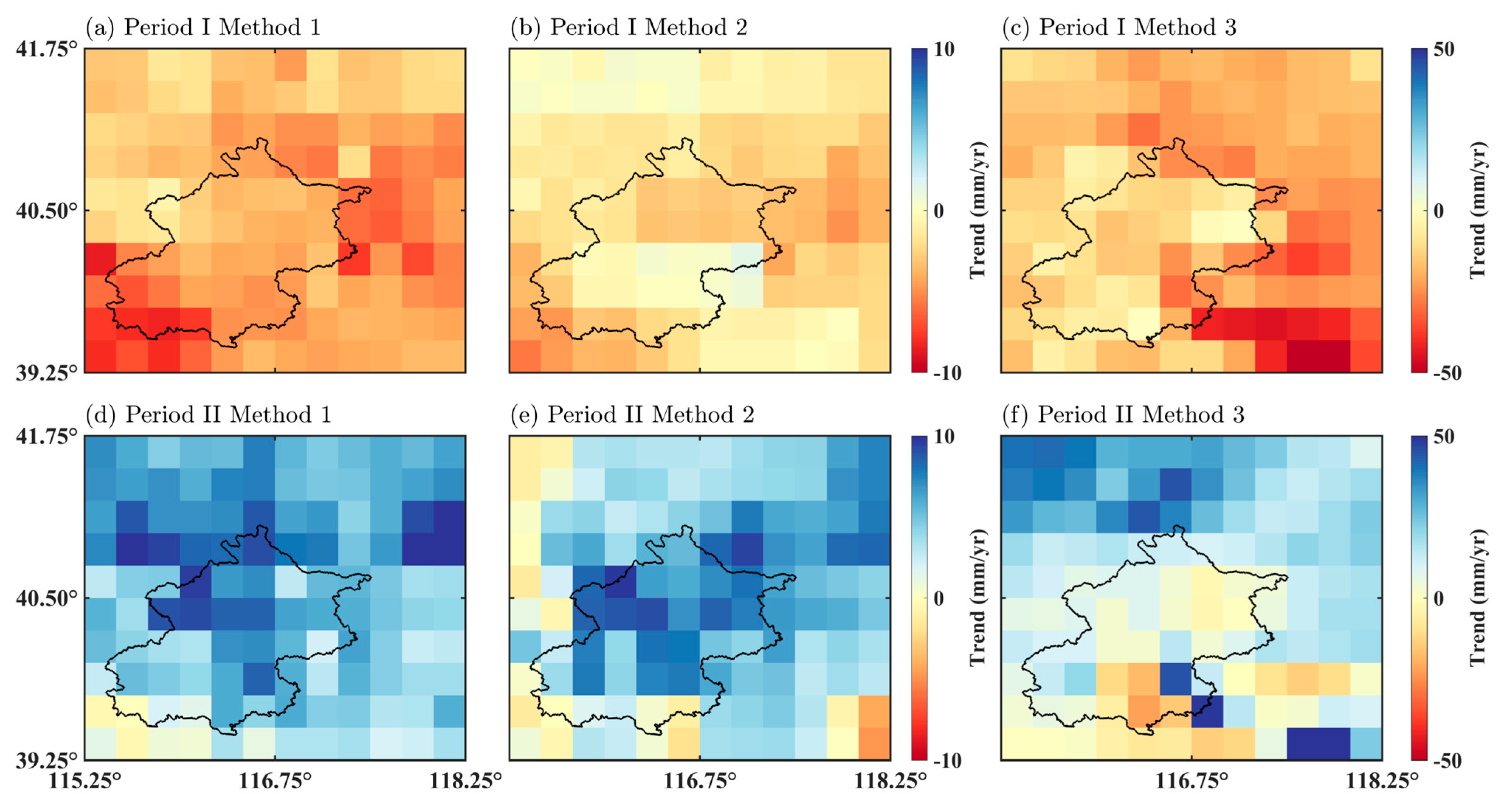
  • On the regional average scale, the trends of GRACE-derived GWSAs in Beijing, estimated based on the three downscaling strategies, are consistent with the trend of measured well data, although the trend rates differ slightly. Before the implementation of SNDWP-MR, the trends all showed decreasing levels, but the rates of decline differed. The downscaled GRACE-derived GWSA based on Method 3 was the closest to the measured well data, at −17.68 ± 4.46 mm/y. After the implementation of the SNDWP-MR, the trends all showed recovering levels; the GRACE-derived GWSA based on Method 3 was also the best, with an increased rate of 10.00 ± 4.77 mm/y.
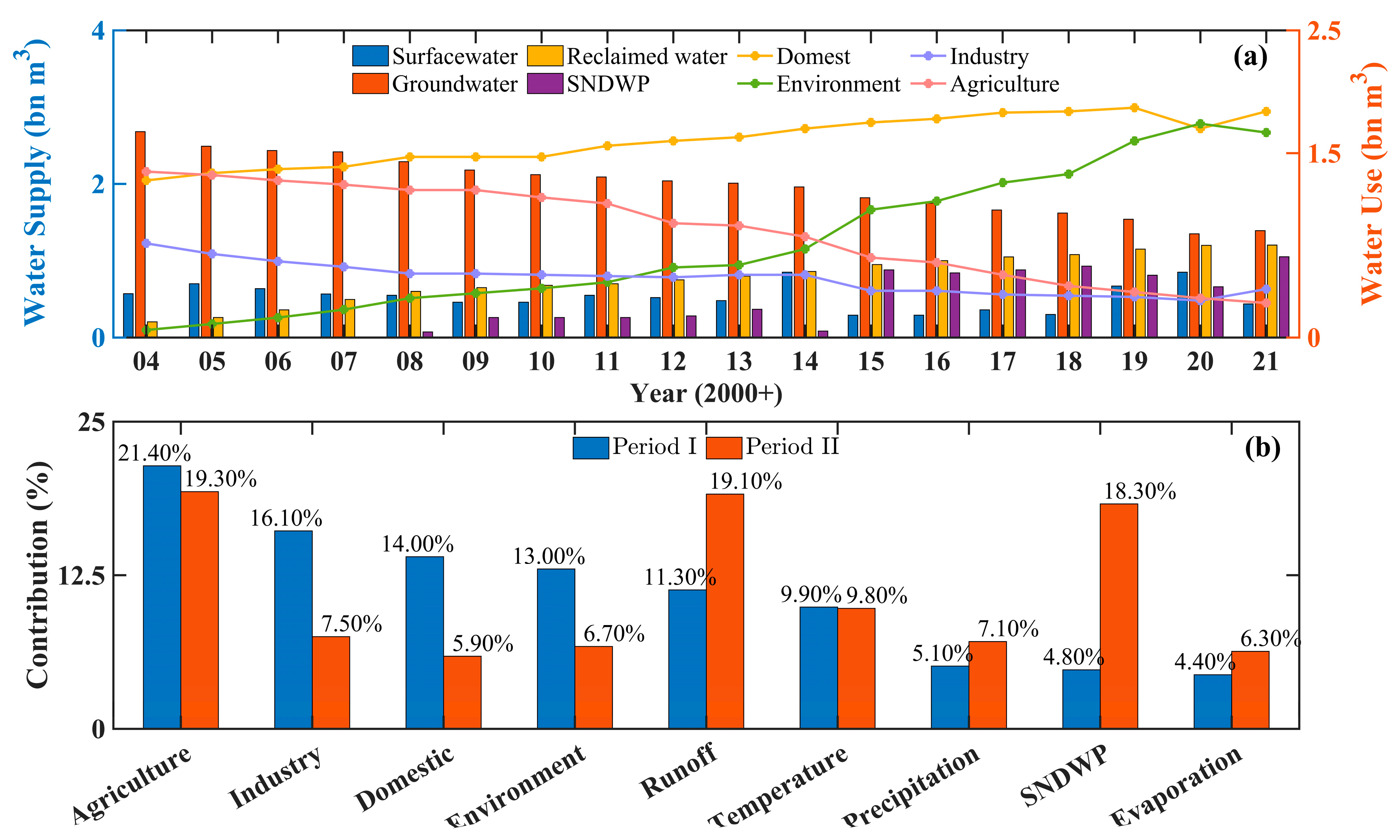
  • Before the implementation of SNDWP-MR, the GWSA in Beijing showed a decreasing trend, to which human factors contributed 69.30% (21.40% for domestic water use and 16.10% for agricultural water use), while climate factors contributed 30.70%. After the implementation of SNDWP-MR, the GWSA showed obvious recovery, to which human factors contributed 57.70% (19.30% attributable to agricultural water use and 18.30% to the SNDWP-MR).
  • The contributions of the GWSA before and after the implementation of SNDWP-MR showed that SNDWP-MR was effective in alleviating groundwater depletion in Beijing.
This study employed multiple strategies to combine GRACE/GRACE-FO with well-monitoring data using DL methods for downscaling to determine the GWSA in Beijing at a spatial resolution of 0.25° × 0.25°. It is significant that the well data not only served as validation data and target variables but was also used as input data to integrate GRACE data for some of the DL models. Additionally, analyzing the GWSA in Beijing as a whole is insufficient for comprehensive monitoring and effective management of underground water resources. The potential of satellite gravity technology to monitor a small-scale GWSA will, therefore, be further explored. To achieve a more detailed understanding of groundwater resources, Beijing should be divided into different hydrogeological units and administrative regions to facilitate the acquisition of high-precision and high-spatial-resolution underground water data. The resulting accumulated dataset will provide new data and technical support for water resource management and decision-making. By considering the individual characteristics of each hydrogeological unit and administrative region, it will be possible to develop improved management strategies and make informed decisions regarding water resources.

Supplementary Materials

The following supporting information can be downloaded at: https://www.mdpi.com/article/10.3390/rs15245692/s1, Figure S1: The structure of LSTM; Figure S2: The structure of GRU; Figure S3: The red grids represent the training grids, the green represents the testing grids, and the number on each grid indicates the grid index; Figure S4: (a) The e r r o r T r a i n and e r r o r T e s t at the 0.5° × 0.5° spatial resolution. The red grids represent the e r r o r T r a i n , the green represents the e r r o r T e s t . (b) The estimated model error of downscaled e r r o r D o w n s c a l e at the 0.25° × 0.25° spatial resolution. Kriging represents Kriging interpolation; Figure S5: The accuracy of training and testing sets for Method 1 and Method 2. “x” represents the training grid cells, and “o“ represents testing grid cells. (a)~(c) Method 1, (d)~(f) Method 2; Table S1: The accuracy of training set for Method 3; Table S2: The accuracy of testing set for Method 3 [65,66,67,68,69].

Author Contributions

Y.H., N.C., J.W. and X.W.: conceptualization, methodology, software. Y.H., N.C., Y.Y. and M.Z.: data curation, writing—original draft preparation. W.Y., J.X., G.D., F.L., Z.W. and G.O.: supervision, reviewing and editing. All authors contributed to the methods, discussions, interpretations, and writing of the paper. All authors have read and agreed to the published version of the manuscript.

Funding

This research was funded by the National Natural Science Foundation of China (Grant No. 41974019 and 42274115), and the Opening Fund of Key Laboratory of Geological Survey and Evaluation of Ministry of Education (Grant No. GLAB2022ZR04 and GLAB2023ZR04).

Data Availability Statement

The data and code of this study are available from the corresponding author upon reasonable request.

Acknowledgments

This study was supported by the National Natural Science Foundation of China (Grant No. 41974019 and 42274115), and the Opening Fund of Key Laboratory of Geological Survey and Evaluation of Ministry of Education (Grant No. GLAB2022ZR04 and GLAB2023ZR04). We thank all the people from CSR, JPL, GSFC, GFZ, NASA LDAS, ECMWF, GLEAM BWA, and CGSB.

Conflicts of Interest

The authors declare that they have no competing interests regarding the publication of this research.

References

  1. Feng, W.; Zhong, M.; Lemoine, J.-M.; Biancale, R.; Hsu, H.-T.; Xia, J. Evaluation of Groundwater Depletion in North China Using the Gravity Recovery and Climate Experiment (GRACE) Data and Ground-Based Measurements. Water Resour. Res. 2013, 49, 2110–2118. [Google Scholar] [CrossRef]
  2. Siebert, S.; Henrich, V.; Frenken, K.; Burke, J. Update of the Digital Global Map of Irrigation Areas to Version 5; Rheinische Friedrich Wilhelms-Universität: Bonn, Germany; Food and Agriculture Organization of the United Nations: Rome, Italy, 2013. [Google Scholar]
  3. Wada, Y.; van Beek, L.P.H.; van Kempen, C.M.; Reckman, J.W.T.M.; Vasak, S.; Bierkens, M.F.P. Global Depletion of Groundwater Resources. Geophys. Res. Lett. 2010, 37, L20402. [Google Scholar] [CrossRef]
  4. Zektser, I.S.; Everett, L.G. Groundwater Resources of the World and Their Use; International hydrological programme; UNESCO: Paris, France, 2004; ISBN 978-92-9220-007-7. [Google Scholar]
  5. Long, D.; Yang, W.; Scanlon, B.R.; Zhao, J.; Liu, D.; Burek, P.; Pan, Y.; You, L.; Wada, Y. South-to-North Water Diversion Stabilizing Beijing’s Groundwater Levels. Nat. Commun. 2020, 11, 3665. [Google Scholar] [CrossRef] [PubMed]
  6. Zhang, Z.; Fei, Y.; Chen, Z.; Zhao, Z.; Xie, Z.; Wang, Y. Others Survey and Evaluation of Groundwater Sustainable Utilization in North China Plain; Geological House: Beijing, China, 2009. [Google Scholar]
  7. Scanlon, B.R.; Faunt, C.C.; Longuevergne, L.; Reedy, R.C.; Alley, W.M.; McGuire, V.L.; McMahon, P.B. Groundwater Depletion and Sustainability of Irrigation in the US High Plains and Central Valley. Proc. Natl. Acad. Sci. USA 2012, 109, 9320–9325. [Google Scholar] [CrossRef] [PubMed]
  8. Döll, P.; Müller Schmied, H.; Schuh, C.; Portmann, F.T.; Eicker, A. Global-Scale Assessment of Groundwater Depletion and Related Groundwater Abstractions: Combining Hydrological Modeling with Information from Well Observations and GRACE Satellites. Water Resour. Res. 2014, 50, 5698–5720. [Google Scholar] [CrossRef]
  9. Rodell, M.; Velicogna, I.; Famiglietti, J.S. Satellite-Based Estimates of Groundwater Depletion in India. Nature 2009, 460, 999–1002. [Google Scholar] [CrossRef] [PubMed]
  10. Zhang, M.; Hu, L.; Yao, L.; Yin, W. Surrogate Models for Sub-Region Groundwater Management in the Beijing Plain, China. Water 2017, 9, 766. [Google Scholar] [CrossRef]
  11. Famiglietti, J.S. The Global Groundwater Crisis. Nat. Clim. Change 2014, 4, 945–948. [Google Scholar] [CrossRef]
  12. Chen, J.; Famigliett, J.S.; Scanlon, B.R.; Rodell, M. Groundwater Storage Changes: Present Status from GRACE Observations. Surv. Geophys. 2016, 37, 397–417. [Google Scholar] [CrossRef]
  13. Xiong, J.; Yin, J.; Guo, S.; Yin, W.; Rao, W.; Chao, N.; Abhishek. Using GRACE to Detect Groundwater Variation in North China Plain after South–North Water Diversion. Groundwater 2022, 61, 402–420. [Google Scholar] [CrossRef]
  14. Tapley, B.D.; Bettadpur, S.; Watkins, M.; Reigber, C. The Gravity Recovery and Climate Experiment: Mission Overview and Early Results. Geophys. Res. Lett. 2004, 31, L09607. [Google Scholar] [CrossRef]
  15. Tapley, B.D.; Watkins, M.M.; Flechtner, F.; Reigber, C.; Bettadpur, S.; Rodell, M.; Sasgen, I.; Famiglietti, J.S.; Landerer, F.W.; Chambers, D.P.; et al. Contributions of GRACE to Understanding Climate Change. Nat. Clim. Change 2019, 9, 358–369. [Google Scholar] [CrossRef] [PubMed]
  16. Feng, W.; Wang, C.; Dapeng, M.; Zhong, M.; Zhong, Y.; Xu, H. Groundwater Storage Variations in the North China Plain from GRACE with Spatial Constraints. Chin. J. Geophys. Acta Geophys. Sin. 2017, 60, 1630–1642. [Google Scholar] [CrossRef]
  17. Zhang, C.; Duan, Q.; Yeh, P.J.-F.; Pan, Y.; Gong, H.; Moradkhani, H.; Gong, W.; Lei, X.; Liao, W.; Xu, L.; et al. Sub-Regional Groundwater Storage Recovery in North China Plain after the South-to-North Water Diversion Project. J. Hydrol. 2021, 597, 126156. [Google Scholar] [CrossRef]
  18. Guo, Y.; Gan, F.; Yan, B.; Bai, J.; Wang, F.; Jiang, R.; Xing, N.; Liu, Q. Evaluation of Groundwater Storage Depletion Using GRACE/GRACE Follow-On Data with Land Surface Models and Its Driving Factors in Haihe River Basin, China. Sustainability 2022, 14, 1108. [Google Scholar] [CrossRef]
  19. Li, H.; Pan, Y.; Huang, Z.; Zhang, C.; Xu, L.; Gong, H.; Famiglietti, J.S. A New GRACE Downscaling Approach for Deriving High-Resolution Groundwater Storage Changes Using Ground-Based Scaling Factors. ESS Open Arch. 2023. [Google Scholar] [CrossRef]
  20. Seyoum, W.; Kwon, D.; Milewski, A. Downscaling GRACE TWSA Data into High-Resolution Groundwater Level Anomaly Using Machine Learning-Based Models in a Glacial Aquifer System. Remote Sens. 2019, 11, 824. [Google Scholar] [CrossRef]
  21. Swenson, S.; Wahr, J.; Milly, P.C.D. Estimated Accuracies of Regional Water Storage Variations Inferred from the Gravity Recovery and Climate Experiment (GRACE). Water Resour. Res. 2003, 39, 1223. [Google Scholar] [CrossRef]
  22. Richey, A.S.; Thomas, B.F.; Lo, M.; Reager, J.T.; Famiglietti, J.S.; Voss, K.; Swenson, S.; Rodell, M. Quantifying Renewable Groundwater Stress with GRACE. Water Resour. Res. 2015, 51, 5217–5238. [Google Scholar] [CrossRef]
  23. Famiglietti, J.S.; Lo, M.; Ho, S.L.; Bethune, J.; Anderson, K.J.; Syed, T.H.; Swenson, S.C.; de Linage, C.R.; Rodell, M. Satellites Measure Recent Rates of Groundwater Depletion in California’s Central Valley. Geophys. Res. Lett. 2011, 38, L046442. [Google Scholar] [CrossRef]
  24. Chao, N.; Luo, Z.; Wang, Z.; Jin, T. Retrieving Groundwater Depletion and Drought in the Tigris-Euphrates Basin Between 2003 and 2015. Groundwater 2018, 56, 770–782. [Google Scholar] [CrossRef]
  25. Yin, W.; Han, S.-C.; Zheng, W.; Yeo, I.-Y.; Hu, L.; Tangdamrongsub, N.; Ghobadi-Far, K. Improved Water Storage Estimates within the North China Plain by Assimilating GRACE Data into the CABLE Model. J. Hydrol. 2020, 590, 125348. [Google Scholar] [CrossRef]
  26. Friis-Christensen, E.; Lühr, H.; Knudsen, D.; Haagmans, R. Swarm—An Earth Observation Mission Investigating Geospace. Adv. Space Res. 2008, 41, 210–216. [Google Scholar] [CrossRef]
  27. Mo, S.; Zhong, Y.; Forootan, E.; Mehrnegar, N.; Yin, X.; Wu, J.; Feng, W.; Shi, X. Bayesian Convolutional Neural Networks for Predicting the Terrestrial Water Storage Anomalies during GRACE and GRACE-FO Gap. J. Hydrol. 2022, 604, 127244. [Google Scholar] [CrossRef]
  28. Li, F.; Kusche, J.; Rietbroek, R.; Wang, Z.; Forootan, E.; Schulze, K.; Lück, C. Comparison of Data-Driven Techniques to Reconstruct (1992–2002) and Predict (2017–2018) GRACE-Like Gridded Total Water Storage Changes Using Climate Inputs. Water Resour. Res. 2020, 56, e2019WR026551. [Google Scholar] [CrossRef]
  29. Long, D.; Shen, Y.; Sun, A.; Hong, Y.; Longuevergne, L.; Yang, Y.; Li, B.; Chen, L. Drought and Flood Monitoring for a Large Karst Plateau in Southwest China Using Extended GRACE Data. Remote Sens. Environ. 2014, 155, 145–160. [Google Scholar] [CrossRef]
  30. Uz, M.; Atman, K.G.; Akyilmaz, O.; Shum, C.K.; Keleş, M.; Ay, T.; Tandoğdu, B.; Zhang, Y.; Mercan, H. Bridging the Gap between GRACE and GRACE-FO Missions with Deep Learning Aided Water Storage Simulations. Sci. Total Environ. 2022, 830, 154701. [Google Scholar] [CrossRef] [PubMed]
  31. Hochreiter, S.; Schmidhuber, J. Long Short-Term Memory. Neural Comput. 1997, 9, 1735–1780. [Google Scholar] [CrossRef]
  32. Chung, J.; Gulcehre, C.; Cho, K.; Bengio, Y. Empirical Evaluation of Gated Recurrent Neural Networks on Sequence Modeling. arXiv 2014, arXiv:1412.3555. [Google Scholar]
  33. Pal, S.K.; Mitra, S. Multilayer Perceptron, Fuzzy Sets, and Classification. IEEE Trans. Neural Netw. 1992, 3, 683–697. [Google Scholar] [CrossRef]
  34. Yin, W.; Hu, L.; Zhang, M.; Wang, J.; Han, S.-C. Statistical Downscaling of GRACE-Derived Groundwater Storage Using ET Data in the North China Plain. J. Geophys. Res. Atmos. 2018, 123, 5973–5987. [Google Scholar] [CrossRef]
  35. Yin, W.; Zhang, G.; Han, S.-C.; Yeo, I.-Y.; Zhang, M. Improving the Resolution of GRACE-Based Water Storage Estimates Based on Machine Learning Downscaling Schemes. J. Hydrol. 2022, 613, 128447. [Google Scholar] [CrossRef]
  36. Wang, Q.; Zheng, W.; Yin, W.; Kang, G.; Huang, Q.; Shen, Y. Improving the Resolution of GRACE/InSAR Groundwater Storage Estimations Using a New Subsidence Feature Weighted Combination Scheme. Water 2023, 15, 1017. [Google Scholar] [CrossRef]
  37. Arshad, A.; Zhang, W.; Zhang, Z.; Wang, S.; Zhang, B.; Cheema, M.J.M.; Shalamzari, M.J. Reconstructing High-Resolution Gridded Precipitation Data Using an Improved Downscaling Approach over the High Altitude Mountain Regions of Upper Indus Basin (UIB). Sci. Total Environ. 2021, 784, 147140. [Google Scholar] [CrossRef] [PubMed]
  38. Ali, S.; Liu, D.; Fu, Q.; Cheema, M.J.M.; Pham, Q.B.; Rahaman, M.; Dang, T.D.; Anh, D.T. Improving the Resolution of GRACE Data for Spatio-Temporal Groundwater Storage Assessment. Remote Sens. 2021, 13, 3513. [Google Scholar] [CrossRef]
  39. Chen, L.; He, Q.; Liu, K.; Li, J.; Jing, C. Downscaling of GRACE-Derived Groundwater Storage Based on the Random Forest Model. Remote Sens. 2019, 11, 2979. [Google Scholar] [CrossRef]
  40. Milewski, A.M.; Thomas, M.B.; Seyoum, W.M.; Rasmussen, T.C. Spatial Downscaling of GRACE TWSA Data to Identify Spatiotemporal Groundwater Level Trends in the Upper Floridan Aquifer, Georgia, USA. Remote Sens. 2019, 11, 2756. [Google Scholar] [CrossRef]
  41. Ning, S.; Ishidaira, H.; Wang, J. Statistical Downscaling of Grace-Derived Terrestrial Water Storage Using Satellite and GLDAS Products. J. JSCE Ser. B1 2014, 70, I_133–I_138. [Google Scholar] [CrossRef]
  42. Sahour, H.; Sultan, M.; Vazifedan, M.; Abdelmohsen, K.; Karki, S.; Yellich, J.; Gebremichael, E.; Alshehri, F.; Elbayoumi, T. Statistical Applications to Downscale GRACE-Derived Terrestrial Water Storage Data and to Fill Temporal Gaps. Remote Sens. 2020, 12, 533. [Google Scholar] [CrossRef]
  43. Sun, J.; Hu, L.; Chen, F.; Sun, K.; Yu, L.; Liu, X. Downscaling Simulation of Groundwater Storage in the Beijing, Tianjin, and Hebei Regions of China Based on GRACE Data. Remote Sens. 2023, 15, 1490. [Google Scholar] [CrossRef]
  44. Huang, Z.; Pan, Y.; Gong, H.; Yeh, P.J.-F.; Li, X.; Zhou, D.; Zhao, W. Subregional-Scale Groundwater Depletion Detected by GRACE for Both Shallow and Deep Aquifers in North China Plain. Geophys. Res. Lett. 2015, 42, 1791–1799. [Google Scholar] [CrossRef]
  45. Liu, R.; Zhong, B.; Li, X.; Zheng, K.; Liang, H.; Cao, J.; Yan, X.; Lyu, H. Analysis of Groundwater Changes (2003–2020) in the North China Plain Using Geodetic Measurements. J. Hydrol. Reg. Stud. 2022, 41, 101085. [Google Scholar] [CrossRef]
  46. Tangdamrongsub, N.; Han, S.-C.; Tian, S.; Schmied, H.M.; Sutanudjaja, E.H.; Ran, J.; Feng, W. Evaluation of Groundwater Storage Variations Estimated from GRACE Data Assimilation and State-of-the-Art Land Surface Models in Australia and the North China Plain. Remote Sens. 2018, 10, 483. [Google Scholar] [CrossRef]
  47. Tao, T.; Xie, G.; He, R.; Tao, Z.; Ma, M.; Gao, F.; Zhu, Y.; Qu, X.; Li, S. Groundwater Storage Variation Characteristics in North China before and after the South-to-North Water Diversion Project Based on GRACE and GPS Data. Water Resour. 2023, 50, 58–67. [Google Scholar] [CrossRef]
  48. Feng, W. GRAMAT: A Comprehensive Matlab Toolbox for Estimating Global Mass Variations from GRACE Satellite Data. Earth Sci. Inform. 2019, 12, 389–404. [Google Scholar] [CrossRef]
  49. Chen, Z.; Zheng, W.; Yin, W.; Li, X.; Ma, M. Improving Spatial Resolution of GRACE-Derived Water Storage Changes Based on Geographically Weight Regression Downscaled Model. IEEE J. Sel. Top. Appl. Earth Obs. Remote Sens. 2023, 16, 4261–4275. [Google Scholar] [CrossRef]
  50. Cheng, M.; Tapley, B.D.; Ries, J.C. Deceleration in the Earth’s Oblateness. J. Geophys. Res. Solid Earth 2013, 118, 740–747. [Google Scholar] [CrossRef]
  51. Geruo, A.; Wahr, J.; Zhong, S. Computations of the Viscoelastic Response of a 3-D Compressible Earth to Surface Loading: An Application to Glacial Isostatic Adjustment in Antarctica and Canada. Geophys. J. Int. 2012, 192, 557–572. [Google Scholar] [CrossRef]
  52. Paulson, A.; Zhong, S.; Wahr, J. Limitations on the Inversion for Mantle Viscosity from Postglacial Rebound. Geophys. J. Int. 2007, 168, 1195–1209. [Google Scholar] [CrossRef]
  53. Long, D.; Pan, Y.; Zhou, J.; Chen, Y.; Hou, X.; Hong, Y.; Scanlon, B.R.; Longuevergne, L. Global Analysis of Spatiotemporal Variability in Merged Total Water Storage Changes Using Multiple GRACE Products and Global Hydrological Models. Remote Sens. Environ. 2017, 192, 198–216. [Google Scholar] [CrossRef]
  54. Martens, B.; Miralles, D.G.; Lievens, H.; van der Schalie, R.; de Jeu, R.A.M.; Fernández-Prieto, D.; Beck, H.E.; Dorigo, W.A.; Verhoest, N.E.C. GLEAM v3: Satellite-Based Land Evaporation and \hack\newlineroot-Zone Soil Moisture. Geosci. Model Dev. 2017, 10, 1903–1925. [Google Scholar] [CrossRef]
  55. Miralles, D.G.; Holmes, T.R.H.; De Jeu, R.A.M.; Gash, J.H.; Meesters, A.G.C.A.; Dolman, A.J. Global Land-Surface Evaporation Estimated from Satellite-Based Observations. Hydrol. Earth Syst. Sci. 2011, 15, 453–469. [Google Scholar] [CrossRef]
  56. The MathWorks, Inc. MATLAB, Version 9.11.0 (R2021b); The MathWorks, Inc.: Natick, MA, USA, 2022. [Google Scholar]
  57. Grimm, R.; Behrens, T.; Märker, M.; Elsenbeer, H. Soil Organic Carbon Concentrations and Stocks on Barro Colorado Island—Digital Soil Mapping Using Random Forests Analysis. Geoderma 2008, 146, 102–113. [Google Scholar] [CrossRef]
  58. Hengl, T.; Nussbaum, M.; Wright, M.N.; Heuvelink, G.B.M.; Graeler, B. Random Forest as a Generic Framework for Predictive Modeling of Spatial and Spatio-Temporal Variables. PEERJ 2018, 6, e5518. [Google Scholar] [CrossRef] [PubMed]
  59. Kuehnlein, M.; Appelhans, T.; Thies, B.; Nauss, T. Improving the Accuracy of Rainfall Rates from Optical Satellite Sensors with Machine Learning—A Random Forests-Based Approach Applied to MSG SEVIRI. Remote Sens. Environ. 2014, 141, 129–143. [Google Scholar] [CrossRef]
  60. Armonk, N.I.C. SPSS, Version 28.0 (R2021); IBM: Armonk, NY, USA, 2021. [Google Scholar]
  61. Humphrey, V.; Gudmundsson, L. GRACE-REC: A Reconstruction of Climate-Driven Water Storage Changes over the Last Century. Earth Syst. Sci. Data 2019, 11, 1153–1170. [Google Scholar] [CrossRef]
  62. Zhao, Q.; Zhang, B.; Yao, Y.; Wu, W.; Meng, G.; Chen, Q. Geodetic and Hydrological Measurements Reveal the Recent Acceleration of Groundwater Depletion in North China Plain. J. Hydrol. 2019, 575, 1065–1072. [Google Scholar] [CrossRef]
  63. Li, P.; Zha, Y.; Shi, L.; Zhong, H. Identification of the Terrestrial Water Storage Change Features in the North China Plain via Independent Component Analysis. J. Hydrol. Reg. Stud. 2021, 38, 100955. [Google Scholar] [CrossRef]
  64. Li, B.; Rodell, M.; Kumar, S.; Beaudoing, H.K.; Getirana, A.; Zaitchik, B.F.; Goncalves, L.G.; Cossetin, C.; Bhanja, S.; Mukherjee, A.; et al. Global GRACE Data Assimilation for Groundwater and Drought Monitoring: Advances and Challenges. Water Resour. Res. 2019, 55, 7564–7586. [Google Scholar] [CrossRef]
  65. Swenson, S.; Chambers, D.; Wahr, J. Estimating geocenter variations from a combination of GRACE and ocean model output. J. Geophys. Res. Solid Earth 2008, 113. [Google Scholar] [CrossRef]
  66. Swenson, S.; Wahr, J. Post-processing removal of correlated errors in GRACE data. Geophys. Res. Lett. 2006, 33. [Google Scholar] [CrossRef]
  67. Bishop, C. Pattern Recognition and Machine Learning (Information Science and Statistics; Springer: New York, NY, USA, 2007. [Google Scholar]
  68. Kumar, K.S.; AnandRaj, P.; Sreelatha, K.; Sridhar, V. Reconstruction of GRACE terrestrial water storage anomalies using Multi-Layer Perceptrons for South Indian River basins. Sci. Total Environ. 2023, 857, 159289. [Google Scholar] [CrossRef] [PubMed]
  69. Berry, M.J.A.; Linoff, G.S. Data Mining Techniques: For Marketing, Sales, and Customer Relationship Management, 2nd ed.; John Wiley & Sons: Hoboken, NJ, USA, 2009. [Google Scholar]
Figure 1. Study area. (a) Location of Hanjiang River basin, Beijing, and North China Plain. The purple line represents the SNDWP-MR. (b) Location of GW monitoring wells. The pink lines are the boundaries of the districts and counties in Beijing.
Remotesensing 15 05692 g001
Figure 2. The methodology flowchart of this study.
Remotesensing 15 05692 g002
Figure 3. The CC, NSE, and RMSE for three DL model-reconstructed GRACE-derived TWSAs compared to the true values of GRACE-derived TWSAs. The left axis represents RMSE, while the right axis represents NSE and CC. (a) LSTM, (b) GRU, and (c) MLP.
Remotesensing 15 05692 g003
Figure 4. The truth values of GRACE-derived TWSAs and reconstructed GRACE-derived TWSAs using LSTM in Beijing from 2004 to 2021. The gray shading represents the 11-month data gap. (a) CSR Mascon, (b) GSFC Mascon, (c) JPL Mascon, (d) CSR SH, (e) GFZ SH, and (f) JPL SH.
Remotesensing 15 05692 g004
Figure 5. Spatial distribution of accuracy and grid scatters density plot between reconstructed TWSAs and their true values. “x” represents the training grid cells, and “o” represents the testing grid cells. The blue line represents the Beijing boundary. The first column is CC, the second column is NSE, the third column is RMSE, and the fourth column is the grid scatter density plot. ((ad) CSR Mascon, (eh) GSFC Mascon, (il) JPL Mascon, (mp) CSR SH, (q–t) GFZ SH, and (ux) JPL SH).
Remotesensing 15 05692 g005
Figure 6. CC, NSE, and RMSE between the GRACE-derived GWSAs before downscaling (0.5° × 0.5°) and in situ GWSAs. (ac) Method 1, (df) Method 2, and (gi) Method 3.
Remotesensing 15 05692 g006
Figure 7. The CC, NSE, and RMSE between the GRACE-derived GWSAs after downscaling (0.25° × 0.25°) and in situ GWSAs from 41 wells. (ac) Method 1, (df) Method 2, and (gi) Method 3.
Remotesensing 15 05692 g007
Figure 8. The downscaled GWSA fitted to the in situ GWSA from the Beijing Plain at the regional average scale and Taylor diagram. (ac) Method 1~Method 3 and (d) Taylor diagram.
Remotesensing 15 05692 g008
Figure 9. The downscaled GRACE-derived GWSA using three methods, in situ GWSA, and precipitation in Beijing on a regional averaged scale. The shade represents uncertainty. (a) Monthly and (b) Yearly.
Remotesensing 15 05692 g009
Figure 10. Spatial distribution of the GRACE-derived GWSA trends before downscaling before and after SNDWP-MR. The first row is the trend before the implementation of SNDWP-MR. (a) Method 1, (b) Method 2, and (c) Method 3. The second row is the trend after the implementation of SNDWP-MR. (d) Method 1, (e) Method 2, and (f) Method 3.
Remotesensing 15 05692 g010
Figure 11. Spatial distribution of the GRACE-derived GWSA trends after downscaling before and after the implementation of SNDWP-MR. The first row is the trends before the implementation of SNDWP-MR. (a) Method 1, (b) Method 2, and (c) Method 3. The second row is the trends after the implementation of SNDWP-MR. (d) Method 1, (e) Method 2, and (f) Method 3.
Remotesensing 15 05692 g011
Figure 12. (a) Water supply (bars) and water use (lines) in Beijing. (b) The contribution of climate factors and human factors.
Remotesensing 15 05692 g012
Table 1. The detailed information of datasets.
VariablesDatasetTime SpanTemporal ResolutionSpatial ResolutionData Source
CSR Mascon TWSACSR RL062002.4~2022.6Monthly0.25° × 0.25°https://www2.csr.utexas.edu/grace/RL06_mascons.html (accessed on 5 October 2023)
GSFC Mascon TWSAGSFC RL062002.4~2022.6Monthly1° × 1°https://earth.gsfc.nasa.gov/geo/data/grace-mascons (accessed on 5 October 2023)
JPL Mascon TWSAJPL RL062002.4~2022.6Monthly0.5° × 0.5°https://grace.jpl.nasa.gov/data/get-data/ (accessed on 5 October 2023)
CSR SH TWSACSR RL062002.4~2022.6Monthly0.25° × 0.25°https://grace.jpl.nasa.gov/data/choosing-a-solution/ (accessed on 5 October 2023)
GFZ SH TWSAGFZ RL062002.4~2022.6Monthly0.25° × 0.25°https://www.gfz-potsdam.de/grace (accessed on 5 October 2023)
JPL SH TWSAJPL RL062002.4~2022.6Monthly0.25° × 0.25°https://grace.jpl.nasa.gov/data/get-data/ (accessed on 5 October 2023)
ERA5-Land PrecipitationERA5-Land1950.1~PresentMonthly0.1° × 0.1°https://cds.climate.copernicus.eu/ (accessed on 5 October 2023)
GLEAM EvapotranspirationGLEAM v31980.1~2021.12Monthly0.25° × 0.25°https://www.gleam.eu/ (accessed on 5 October 2023)
CLSM TWSACLSM L42003.2~2022.12Daily0.25° × 0.25°https://ldas.gsfc.nasa.gov/gldas (accessed on 5 October 2023)
CLSM RunoffCLSM L42003.2~2022.12Daily0.25° × 0.25°https://ldas.gsfc.nasa.gov/gldas (accessed on 5 October 2023)
CLSM TemperatureCLSM L42003.2~2022.12Daily0.25° × 0.25°https://ldas.gsfc.nasa.gov/gldas (accessed on 5 October 2023)
CLSM SMSCLSM L42003.2~2022.12Daily0.25° × 0.25°https://ldas.gsfc.nasa.gov/gldas (accessed on 5 October 2023)
CLSM CNSCLSM L42003.2~2022.12Daily0.25° × 0.25°https://ldas.gsfc.nasa.gov/gldas (accessed on 5 October 2023)
CLSM SNSCLSM L42003.2~2022.12Daily0.25° × 0.25°https://ldas.gsfc.nasa.gov/gldas (accessed on 5 October 2023)
In situ Groundwater Level\2005.1~2016.12
2004~2021
Monthly/Yearly41 Wellshttps://swj.beijing.gov.cn/ (accessed on 5 October 2023)
https://en.cgs.gov.cn/ (accessed on 5 October 2023)
Table 2. CC, NSE, and RMSE between the truth values of GRACE-derived TWSAs and reconstructed GRACE-derived TWSAs during the training and testing periods.
GRACEErrorsTrain Period (2004~2015)Test Period (2016~2021)
CSR MasconCC0.990.88
NSE0.980.76
RMSE (mm)6.1614.46
GSFC MasconCC0.970.84
NSE0.980.71
RMSE (mm)7.8316.16
JPL MasconCC0.990.83
NSE0.980.68
RMSE (mm)8.0014.16
CSR SHCC0.960.86
NSE0.930.73
RMSE (mm)8.7714.68
GFZ SHCC0.950.87
NSE0.910.72
RMSE (mm)12.5614.05
JPL SHCC0.990.84
NSE0.980.70
RMSE (mm)4.2713.78
Table 3. Trends of the downscaled GWSA during Period I and Period II.
Trend (mm/y) *Method 1Method 2Method 3
Period I (2004~2014)−4.07 ± 1.60−4.39 ± 2.48−17.68 ± 4.46
Period II (2015~2021)5.04 ± 5.0020.25 ± 7.4010.00 ± 4.77
‘*’ indicates the trend is significant at a 95% level.
Disclaimer/Publisher’s Note: The statements, opinions and data contained in all publications are solely those of the individual author(s) and contributor(s) and not of MDPI and/or the editor(s). MDPI and/or the editor(s) disclaim responsibility for any injury to people or property resulting from any ideas, methods, instructions or products referred to in the content.

