Multi-Satellite Observation-Relay Transmission-Downloading Coupling Scheduling Method

Abstract

With the development of satellite cluster technology, the earth observation capability of satellite clusters has been greatly enhanced, along with the improvement of satellite earth observation and inter-satellite data transmission ability. Nevertheless, it is difficult to coordinate satellite observation, inter-satellite data transmission, and satellite–ground data download to satisfy the constraints of satellite multi-subsystems. In this article, the multi-satellite observation-relay transmission-downloading coupling scheduling problem is described. Based on the conventional tabu search algorithm for multi-satellite earth observation, the data transmission path planning algorithm is integrated to carry out the entire coupling process of multi-satellite observation, inter-satellite data transmission, and satellite–ground data downloading. Referring to the idea of the artificial potential field method, the satellite cluster profit-state evaluation function is introduced to enhance the local search process within the tabu search framework. Moreover, in the data transmission planning algorithm, the rule-based Dijkstra data transmission path planning method is proposed based on two data transmission path planning strategies and the satellite cluster state-strategy selection rules. The simulation results show that the proposed method can realize the entire process of scheduling satellite cluster observation, relay transmission, and downloading and enhance the ability of the satellite cluster to obtain observation data. The improved Dijkstra method enhances the adaptability of the data transmission path planning method to the multi-subsystem coupled problem, and the improved local search in the tabu search method elevates the searching capability of the algorithm.

1. Introduction

The earth observation satellite (EOS) acquires Earth’s surface data from space, offering the advantage of extensive detection coverage. EOS finds widespread applications in disaster monitoring, environmental surveillance, and resource exploration [1]. Accompanying the increment in the number of in-orbit satellites, the collaboration of multiple EOSs has strengthened the Earth’s observation ability, expanded coverage, and increased the number of observation targets, which is beyond what a single EOS could accomplish. Typical multi-EOS projects include Pleiades [2], World View [3], HJ [4], etc. Multi-EOS mission scheduling involves the rational scheduling of on-board actions during satellite observation processes to maximize profit while satisfying the satellite’s constraints [5]. Based on single-EOS mission scheduling, multi-EOS mission scheduling also needs to schedule multi-EOS cooperative work [6]. In recent years, the multi-EOS scheduling problem has received extensive attention and research efforts.

The process of satellite earth observation involves capturing ground target information through a camera, storing it in storage, and subsequently transmitting it to a ground station. The observation data acquisition ability and data transmission of a single satellite are constrained by the satellite-station data transmission window and satellite storage capacity. With the continuous advancement of satellite communication technology, the number of satellites capable of inter-satellite communication is increasing, and the inter-satellite data transmission capacity is constantly improving. Projects such as Starlink, OneWeb, and Telesat [7] exhibit strong inter-satellite data communication capabilities. Inter-satellite data transmission enables observation satellites to relay data to ground stations through other satellites when they are not within the satellite-station data transmission window, thereby reducing the occupancy of satellite storage resources and enhancing their target observation capabilities. Integrating multiple capabilities in a single satellite, including target observation, inter-satellite data transmission, and satellite-ground data transmission, is a development trend, as it can maximize the collective capabilities of the satellite cluster. However, this integration also presents scheduling challenges for the satellite cluster. The processes of multi-satellite observation, inter-satellite data transmission, and satellite-ground data downloading are coupled, and they are coupled in terms of electricity consumption and storage occupancy. Effectively coordinating the entire coupled process of multi-satellite observation, relay transmission, and downloading is the key to the problem. In prior research, scholars have conducted investigations into the single-satellite observation scheduling problems [8,9,10,11,12,13], the multi-satellite observation scheduling problems [14,15,16,17], the schedule problems of multi-satellite observation and downloading data through a single satellite [18,19,20,21], and the multi-satellite data relay transmission scheduling problems [22,23,24,25]. There is relatively limited research that discusses multi-satellite observation and the entire coupled process involving multi-satellite observation, relay transmission, and data downloading. Therefore, this article delves into the study of the coupled scheduling problem for the entire process of multi-satellite observation, relay transmission, and downloading.

The multi-satellite observation-relay transmission-download coupling scheduling problem includes the multi-satellite observation scheduling process and the data transmission planning process, whereas the data transmission planning process includes determining which satellite will be involved in the process of transmitting observation data between satellites and which satellite will be responsible for downloading the data to the ground station. The multi-subsystem constraints, including attitude maneuvering constraints, electricity subsystem constraints, data transmission subsystem constraints, etc., are considered in the scheduling problem. To address the multi-satellite observation-relay transmission-download coupling scheduling problem, a multi-satellite data transmission path planning method is incorporated into the conventional multi-satellite observation scheduling method in this article. In the multi-satellite observation-relay transmission-download coupling scheduling problem, the target is relatively fixed while the ground station and satellites’ orbits are fixed. Although the motion parameters of satellites, the relative position of a satellite to a target, and the relative position of a satellite to a ground station change during the observation process, these changes are regular and can be converted into fixed relationships through pre-processing calculations. These relationships include the observation time window of a satellite to a target, the data transmission time window of a satellite to a ground station, the inter-satellite link topology, etc. The data transmission path planning problem is different from the network routing path planning problem [26]. In the network routing path planning problem, dynamic factors, including varying network load, transmission delay, and network bandwidth, are required to be considered in the routing algorithm because of the varying service flow and the number of access users. However, for the data transmission path planning process in the multi-satellite observation-relay transmission-download coupling scheduling problem, the inter-satellite and satellite-ground data transmission windows are determined by the initial distribution of satellites and ground stations, and network topology changes can be predicted. At the same time, inter-satellite and satellite-to-ground data transmissions are point-to-point transmissions, resulting in relatively minor variations in bandwidth and network load. Therefore, in this article, the variation of dynamic parameters in the communication process is not the main contradiction. In this context, calculating inter-satellite and satellite-ground data transmission time windows during preprocessing, scheduling the order of data transmission nodes, and arranging data transfer events is a common method in observation data transmission planning [27]. The data transmission path planning problem is considered the data transmission node path selection certainty problem in this article, which can meet the demand for the solution of the data transmission planning process in the multi-satellite observation-relay transmission-download coupling scheduling problem. In this case, combined with the reliability requirements in the astronautic field, the classic Dijkstra method [28] is applied to solve the problem of data transmission path planning. When solving the data transmission path planning problem, in certain scenarios, it is necessary to download the observation data earlier to reduce the occupation of data transmission resources, whereas in other scenarios, the number of data relay satellite nodes needs to be minimized to reduce satellite electric energy consumption, in which case the path search strategy has to be changed according to the satellite cluster states. To cope with different scenarios, the appropriate data transmission path selection under different satellite cluster states is achieved by formulating different node distance calculation rules and selecting the path according to the distance calculation rules in specific satellite cluster states.

The multi-satellite observation-relay transmission-download coupling scheduling process is complex, large-scale, and also involves numerous subsystem constraints. There is coupling and mutual influence among the subsystems of the satellite. In multi-satellite observation scheduling, commonly used methodologies include exact methods, heuristic methods, and metaheuristic methods [29]. The exact method [30,31,32,33] can obtain the optimal solution, but the efficiency of the algorithm is significantly reduced when the task size is increased [29], which is not suitable for the large-scale multi-satellite observation-relay transmission-download coupling scheduling problem. The heuristic method [34,35,36] has high problem-solving efficiency; however, it is only suitable for specific scenarios due to fixed rules. The multi-satellite observation-relay transmission-download coupling scheduling problem is affected by multiple factors such as observation, data transmission, and multi-subsystem constraints. Changes in the scenario may lead to suboptimal algorithmic results. Metaheuristic methods use a search-based approach, achieving a balance between efficiency and obtaining better results. Common metaheuristic approaches for satellite mission planning include genetic algorithms, simulated annealing algorithms, ant colony optimization, tabu search, etc. A genetic algorithm [37,38] uses genetic operators to achieve optimization by imitating the process of population reproduction and has strong global search ability. Traditional genetic algorithms have a low convergence speed, and blind searches easily result in low efficiency or repeated searches. This phenomenon is more obvious when genetic algorithms solve large-scale problems [25]. Slow convergence is exacerbated in the context of entire process coupling planning and intricate subsystem interactions. Using a genetic algorithm in the multi-satellite observation-relay transmission-download coupling scheduling problem will also result in low convergence speed, as this is a large-scale problem that contains complex processes and numerous subsystem constraints. Ant colony optimization [39,40] has the advantage of fast convergence brought by positive feedback, but due to the accumulation of pheromones, it can easily fall into local optimization [41]. Because of the complexity of the multi-satellite observation-relay transmission-download coupling scheduling problem, the disadvantage that the ant colony algorithm is easy to fall into the local optimum will also be aggravated here. The simulated annealing method [42,43] has both global search ability and local search ability by controlling the temperature-decreasing speed. However, a very slow decrease in temperature gives the best results but is also computationally costly. If the temperature is decreased too rapidly, the system is likely to become trapped in a local minimum [44]. The solution process for the multi-satellite observation-relay transmission-download coupling scheduling problem is related to the target distribution, the ground station distribution, the number, and the states of satellites. When using the simulated annealing method in the multi-satellite observation-relay transmission-download coupling scheduling problem, it is required to set reasonable parameters for different scenarios, bringing difficulties to applying this method. Tabu search [45,46,47,48] avoids cycling by storing the information of the past in the search. It usually reaches local minima since a single candidate solution is used to generate offspring [49]. It is also highly inclined to fall into the local optimum in the multi-satellite observation-relay transmission-download coupling scheduling problem.

The multi-satellite observation-relay transmission-download coupling scheduling problem brings challenges to solution searching, but the rational use of the coupling law between the subsystems can also play a role in guiding the search process. By guiding the search direction to change the states of the satellite subsystem and reasonably allocating the missions, the resources of the subsystems of the satellite can be reasonably used to complete more target observations and data transmission. The key to solving the problem lies in reasonable neighborhood design and the formulation of the neighborhood search strategy. In previous studies, He [45] used the tabu search algorithm in the satellite observation mission scheduling problem, designing neighborhoods of insertion, deletion, exchange, and rearrangement. These types of search neighborhoods have good adaptability in solving the satellite observation scheduling problems that can be associated with the state changes of the satellite subsystem. Referring to the idea of the artificial potential field method [50,51,52,53], the traditional tabu search method for satellite observation scheduling is improved in this article. In the searching process, different satellite cluster states are distinguished, while different neighborhood selection rules are adopted for different states. The state evaluation function of the cluster efficiency subsystem is established to control the search direction and adjust the state of each subsystem of the satellite cluster, which helps the traditional tabu search algorithm overcome the local optima problem, thus improving the search method.

In this article, the multi-satellite observation-relay transmission-downloading coupling scheduling problem is described. Based on the tabu search algorithm for the multi-satellite observation scheduling problem [45], the data transmission path planning method for observation missions is incorporated to solve the scheduling problem. The contributions to this article are as follows:

• In the neighborhood selection process of the tabu search algorithm, a system state evaluation function is introduced, and local search improvement rules based on satellite states are formulated to improve the local search direction according to the artificial potential field method;
• In the data transmission path planning process, two data transmission path selection strategies are designed based on the Dijkstra algorithm. Rules for selecting the problem-solving strategy are established based on the satellite cluster state, thereby enabling adaptive satellite data transmission path planning based on the satellite cluster’s state.

The remainder of this paper is organized as follows: Section 2 defines the multi-satellite observation-relay transmission-downloading scheduling problem, while Section 3 describes the improved tabu search method for multi-satellite observation-relay transmission-download coupling scheduling. Furthermore, Section 4 presents the simulation scenarios and results. Discussions are carried out in Section 5, and Section 6 concludes this paper.

2. Problem Description

The multi-satellite observation-relay transmission-downloading process entails satellites using cameras to observe target information and storing observation data in storage. Subsequently, during overpasses of ground stations, they download stored data. Alternatively, they may relay the observation data to other satellites for subsequent downloading. The observation target type in this research is the point targets that are fixed on the Earth’s surface. The mission scheduling process involves multi-satellite observation, mission allocation, and observation data transmission path planning. In the problem studied in this paper, each satellite in the satellite cluster can engage in observation operations as well as receive, transmit, and download target observation data, serving as a relay data transmission satellite when necessary. This creates a coupling of the entire multi-satellite observation-relay transmission-downloading process. The working process of the satellite cluster is shown in Figure 1. The multi-satellite observation-relay transmission-downloading scheduling problem is defined as a mixed-integer programming problem. Parameters that are involved in the scheduling problem are shown in

Table 1. Parameters in the problem description.

Parameter	Meaning
nt	The number of targets
nr	The number of satellites
ns	The number of ground stations
i, j	The index of targets
k, l	The index of satellites
m	The index of ground stations
ts, te	The start time and end time of the scheduling
towskio, towekio	Satellite k’s start time and end time for the oth observation time window of target i, with the total number of observation time windows being nowki
trwsklp, trweklp	Satellite k’s start time and end time for the pth inter-satellite data transmission time window to satellite l. The total number of inter-satellite data transmission time windows is nrwkl, and the windows between two satellites are mutual; thus, nrwkl = nrwlk, trwsklp = trwslkp, trweklp = trwelkp.
tdwskmq, tdwekmq	Satellite k’s start time and end time for the qth satellite-ground data transmission time window to ground station m. The total number of satellite-ground data transmission time windows is ndwkm.
toski, toeki	Satellite k’s observation start time and end time for target i.
tdskmi, tdekmi	Satellite k’s start time and end time for transmitting observation data of target i to ground station m.
trOutskli, trOutekli	Satellite k’s start time and end time for transmitting observation data of target i to satellite l. The transmitting direction is satellite k to satellite,
trInskli, trInekli	Satellite l’s start time and end time for receiving data of target i from satellite k. The transmitting direction is satellite k to satellite l. The transmission time of satellite k for transmitting observation data of target i to satellite l is the same as the time when satellite l receives target i’s observation data from satellite k, i.e., trOutskli = trInskli, and trOutekli = trInekli.
$\Delta t_o$	The observation time of single target
$\Delta t_{Ai,j}$	The attitude maneuver time required for observation missions’ attitude transition of satellite k
$\Delta t_{prk}$	The device switching time between two inter-satellite data transmission missions to different satellites of satellite k
$\Delta t_{pdk}$	The device switching time between two data downloading missions to different ground stations of satellite k
Wk, WkTotal	Satellite k’s the available electrical energy and satellite k’s electrical energy capacity of the battery.
Mk, MkTotal	Satellite k’s occupied memory capacity and satellite k’s total memory capacity.

.

The decision variables are as follows:

$\begin{array}{cc}{x}_{ki}\in \left\{0,1\right\}& i=1,2,\dots ,n_t\end{array},k=1,2,\dots ,n_r$ represents whether satellite k observes target i.

$\begin{array}{cc}{g}_{ki,j}\in \left\{0,1\right\}& i,j=1,2,\dots ,n_t,k=1,2,\dots n_r\end{array}$ represents whether satellite k’s observation order for targets i and j, where g_ki,j = 1 indicates that satellite k observes target i and target j in an adjacent order, with target j observed after target i.

$\begin{array}{cc}{y}_{ik,l}\in \left\{0,1\right\}& i=1,2,\dots ,n_t\end{array},k,l=1,2,\dots ,n_r$ represents whether satellite k transfers data of target i to satellite l, with the direction of transmission from satellite k to satellite l.

$\begin{array}{cc}{z}_{ikm}\in \left\{0,1\right\}& i=1,2,\dots ,n_t,k=1,2,\dots ,n_r,m=1,2,\dots ,n_s\end{array}$ represents whether satellite k transfers data of target i to ground station m.

The objective function of the problem can be expressed as

$$J={\displaystyle \sum _{i=1}^{n_t}\left(v_i{\displaystyle \sum _{k=1}^{n_r}{\displaystyle \sum _{m=1}^{n_s}{z}_{ikm}}}\right)},$$

(1)

where J is the objective function value, the profit v_i of target i can be described as its value to the users and its importance to the targets. The higher the weighted sum of the target values, the greater the overall benefit. The objective function signifies the weighted profit of all targets observed, transmitted, and ultimately downloaded to the ground station by the satellite cluster.

The observation time window and the data transmission time window in the problem description are calculated through the preprocessing process and the state calculation process. In this article, the satellites are agile, capable of adjusting their attitude through pitch and roll maneuvers to observe targets within their field of view. The observation time window for a satellite to observe a target represents the earliest and latest times during which the satellite can observe the target within the allowable range of satellite attitude maneuvers. The observation time window [t_owskio, t_owekio] is calculated based on the relative position between satellite k and target i, considering the satellite’s maximum allowable maneuver cone angle constraints. The satellite-ground data transmission time window [t_dwskmq, t_dwekmq] is the period when the kth satellite’s antenna and the mth ground station’s antenna are visible to each other. During the satellite-ground data transmission time window, the satellite can download data to the ground station. The calculation of the satellite-ground data transmission time window relies on satellite orbital information and attitude history A_k(t). Similarly, the inter-satellite data transmission time window [t_rwsklp, t_rweklp] is the period when satellite k and satellite l are visible to each other. During the time window, an inter-satellite link can be established between the two satellites for data transmission.

The constraints that should be considered in the mission scheduling problem are as follows:

$$\begin{array}{cc}{t}_{oski}\ge t_{owskio}\wedge t_{oeki}\le t_{owekio}& \exists o,1\le o\le n_{owki}\end{array},$$

(2)

$$\begin{array}{cc}{t}_{oskj}-t_{oeki}\ge \Delta t_{Ai,j}& g_{ki,j}=1\end{array},$$

(3)

$$\{\begin{array}{cc}\begin{array}{c}{t}_{rOutskli}\ge t_{rwsklp}\wedge t_{rOutekli}\le t_{rweklp}\\ t_{rInskli}\ge t_{rwsklp}\wedge t_{rInekli}\le t_{rweklp}\end{array}& \exists p,1\le p\le n_{rwkl}\end{array},$$

(4)

$$\begin{array}{cc}{t}_{dskmi}\ge t_{dwskmq}\wedge t_{dekmi}\le t_{dwekmq}& \exists q,1\le q\le n_{dwkm}\end{array},$$

(5)

$$\{\begin{array}{cc}\left[t_{rOutskli},t_{rOutekli}\right)\cap \left[t_{rOutsklj},t_{rOuteklj}\right)=\varphi & \forall l,i,j,i\ne j\\ \left[t_{rOutsk{l}_{1}i}-\Delta t_{prk{l}_1},t_{rOutek{l}_{1}i}\right)\cap \left[t_{rOutsk{l}_{2}j}-\Delta t_{prk{l}_2},t_{rOutek{l}_{2}j}\right)=\varphi & \forall l_1,l_2,l_1\ne l_2\end{array},$$

(6)

$$\{\begin{array}{cc}\left[t_{dskmi},t_{dekmi}\right)\cap \left[t_{dskmj},t_{dekmj}\right)=\varphi & \forall m,i,j,i\ne j\\ \left[t_{dsk{m}_{1}i}-t_{pdk},t_{d\mathrm{e}k{m}_{1}i}\right)\cap \left[t_{dsk{m}_{2}j}-t_{pdk},t_{dek{m}_{2}j}\right)=\varphi & \forall m_1,m_2,m_1\ne m_2\end{array},$$

(7)

$$\{\begin{array}{c}{y}_{ik,l}\le x_{ki}\\ y_{i{k}_2,k_3}\le y_{i{k}_1,k_2}\\ z_{ikm}\le x_{ki}\\ z_{ikm}\le y_{il,k}\end{array},$$

(8)

$$t_{rOuts{k}_2{k}_{3}i}\ge t_{rIne{k}_1{k}_{2}i},$$

(9)

$$\{\begin{array}{c}{t}_{dskmi}\ge t_{oeki}\\ t_{dskmi}\ge t_{rInelki}\end{array},$$

(10)

$$0\le W_k\le W_{Totalk},$$

(11)

$$0\le M_k\le M_{Totalk}.$$

(12)

Equation (2) represents the observation time window constraint, which means that a satellite’s observation must occur within the observation time window. Equation (3) is the attitude maneuver constraint, which means that the observation time interval between two adjacent missions of a single satellite needs to be greater than the attitude maneuver conversion time of the observation attitude of the two observation missions.

Equation (4) represents the inter-satellite data transmission time window constraint. It signifies that the inter-satellite data transmission must occur within the inter-satellite data transmission time window. Equation (5) represents the satellite-ground data transmission time window constraint. It dictates that a satellite’s data downloading operations must align with the requirements of the satellite-ground data transmission time window.

Equations (6) and (7) correspond to the data transmission switch time constraint, which means that when a satellite is performing data transmission to different satellites, there should be an interval between two transmission missions for data transmission equipment preparation. Similarly, for data downloading to ground stations, if the data is transmitted to two different ground stations, an interval must exist between the two transmission missions to accommodate the data transmission equipment preparation time, where $\Delta t_{prkl}=\max \left(\Delta t_{prk},\Delta t_{prl}\right)$.

Equation (8) represents the data transmission logical constraint, signifying that the premise of data forwarding and downloading is the completion of the observation or data reception. Equations (9) and (10) are the timing constraints of data transmission, which means that the start time of inter-satellite data transmission or satellite-ground data downloading must be greater than the end time of observation or data reception.

Equation (11) represents the electricity constraint. In this equation, W_k represents the current electric energy of satellite k, and the formula for W_k calculation is

$$W_k=W_{Initialk}+{\displaystyle \int \left(P_{Ink}-P_{Camk}-P_{GroundDataTransk}-P_{SatelliteDataTransk}-P_{Attitudek}\right)}dt,$$

(13)

where W_Initialk represents the initial electricity energy of satellite k. P_Ink stands for the charging power of satellite k. The charging power is calculated based on the angle between the satellite’s solar panels’ normal vector and the sunlight vector, which changes with the satellite’s attitude. P_Camk is the consumption power for satellite k observation; a satellite consumes electric energy while observing a target. P_{SatelliteDataTransk} is the consumption power of satellite k during inter-satellite data transmission, where both data transmission input and output consume electric energy. P_{GroundDatatransk} is the consumption power of satellite k during satellite-ground data transmission. A satellite consumes electricity while downloading data to ground stations. P_Attitudek represents the consumption power of satellite k during attitude maneuvers. The formulas indicate that satellite observations, inter-satellite data transmission, satellite-ground data downloading, and attitude maneuvers all consume electrical power. This reflects the coupling of electricity and energy consumption between satellite observations and data transmission activities.

Equation (12) represents the memory constraint; the occupied memory of storage is calculated as

$$\begin{array}{cc}{M}_k={\displaystyle \int \left(R_{CamInk}t+R_{SatDataTransInlk}t-M_{\mathrm{era}}\left(t\right)\right)}dt& y_{il,k}=1\end{array},$$

(14)

where R_CamInk represents the data rate generated by the camera for capturing images, and R_{SatDataTransInlk} represents the code rate for inter-satellite data transmission between satellite l and satellite k, which is the smaller of the two satellite transmission code rates. The observation and the data reception increase the occupied memory.

The memory-erase event clears individual files; each observation of a target forms an image data file. During the processes of storing, transmitting, and erasing observation image data for a target, complete image data files need to be stored, transmitted, and erased. The satellite memory erase time is scheduled after the data are transmitted to other satellites or downloaded to the ground station. The occupied memory decreases correspondingly after data erasing. The equation reflects the memory occupancy coupling of satellite observations and data transmission. The calculations for attitude maneuver history, observation time window, data transmission time window, W_k, and M_k can be found in reference [54].

3. Improved Tabu Search Method for Multi-Satellite Observation-Relay Transmission-Download Coupling Scheduling

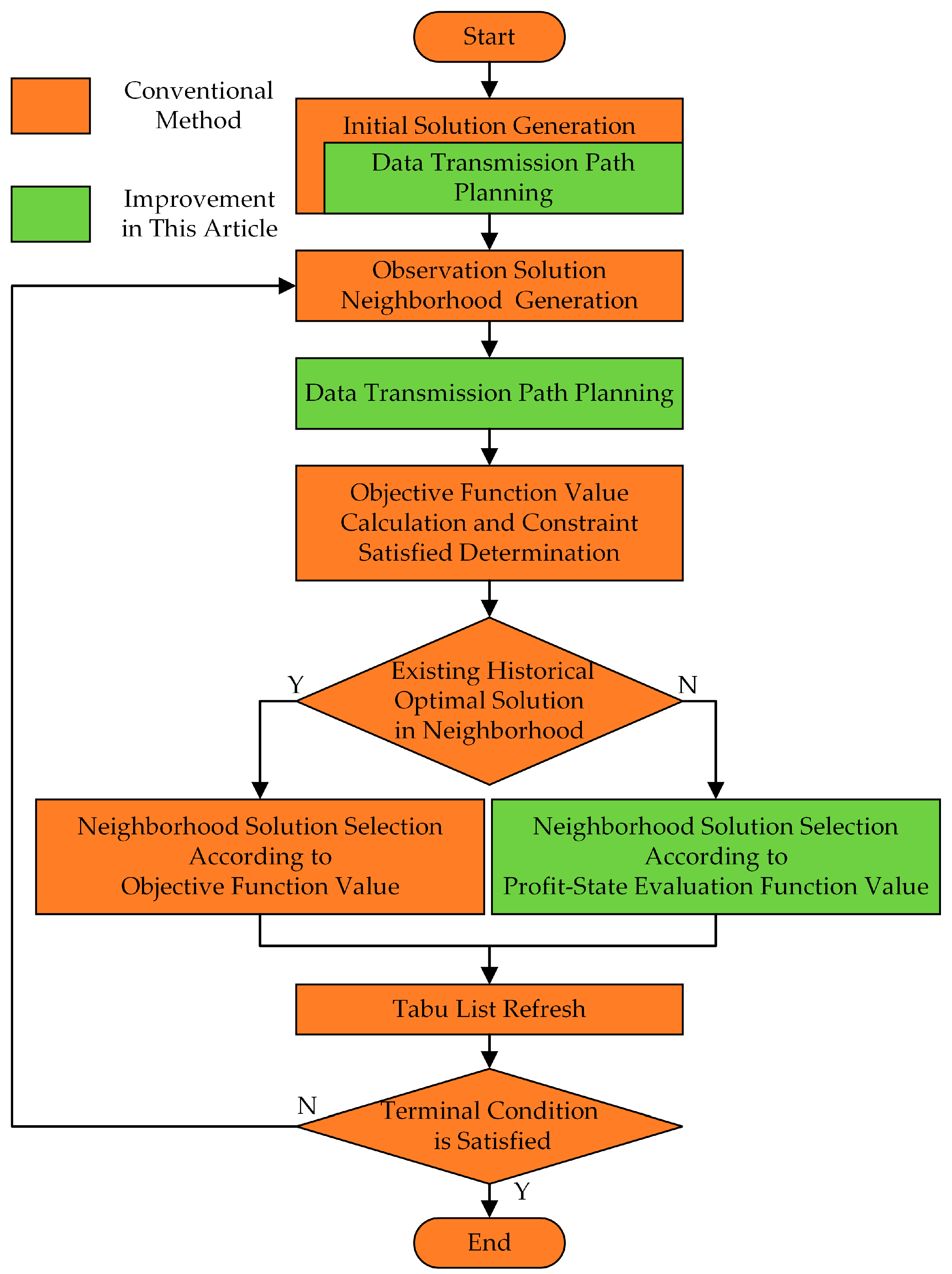
3.1. Method Framework

The main improvements introduced in this article are primarily focused on two aspects: 1. Improvement of the local search process in tabu search; 2. Improvement of the data transmission path planning method based on observation solutions. The method framework and the improvements in the method are reflected in Figure 2, and the process is as follows:

• Generate an initial solution using the initial solution generation method, and use this initial solution as the current solution. The process of the initial solution is described in Section 3.2;
• Generate observational neighborhood solutions based on the current solution and the local search rules;
• Determine the attitude maneuver constraint satisfaction of observation neighborhood solutions and generate the attitude maneuver history of neighborhood solutions. Calculate the inter-satellite data transmission time windows and satellite-ground data transmission time windows. Generate inter-satellite data transmission solutions y_ik,l and satellite-ground downloading solutions z_ikm through the data transmission plan method based on the observation neighborhood solutions. Calculate the satellite cluster’s status and keep all solutions that satisfy all constraints. The data transmission path plan method is described in Section 3.4. The data transmission path plan method is also used in the initial solution generation method to generate the data transmission solution of the initial observation solution;
• Evaluate the neighborhood solutions using the objective function value J. If there is a historically optimal solution in the neighborhood solutions, it is selected as the current solution and updated in the algorithm; otherwise, evaluate the neighborhood solutions using the satellite cluster profit-state evaluation function and use the historically optimal solution or current non-tabu best solution based on profit-state evaluation values as the current solution. Details related to the improvement of the observation local search process are described in Section 3.3;
• Update the tabu list;
• Repeat steps 2–5 until the algorithm termination condition is met. Output the historically optimal solution.

3.2. Initial Solution Generation Method

The process of generating initial solutions follows the strategy of maximum backward time slack [55], which is a heuristic rule aiming to maximize the number of observed targets. The process for generating initial solutions is as follows:

• All targets form the unselected target set;
• Select each target from the unselected set to perform mission insertion into each insertion position of each satellite’s current observation result sequence to generate a set of observation solution candidates;
• Calculate the sequence backward time slack of the inserted satellite for all observation solution candidates;
• Sort solutions in descending order of the backward time slack. Keep the observation solutions that meet the attitude maneuver constraint. If all solutions to a target do not meet the attitude maneuver constraint, remove the target from the unselected target set. If there is no solution remaining, go to step 8;
• Select an observation solution according to the sorting order and plan the data transmission path. Verify the constraint satisfaction of the observation solution. The data transmission path planning method is described in Section 3.4;
• If the selected solution satisfies the constraint, insert it into the satellite observation sequence according to the corresponding position and go to step 7. Otherwise, if all solutions to the selected target do not meet the constraints, remove the target from the unselected target set. In the unsatisfied situation, if there is an unprocessed observation solution, go to step 5; otherwise, go to step 7;
• If there is a target in the unselected target set, go to step 2; otherwise, go to step 8;
• End.

The solution can be further improved through the tabu search algorithm based on the initial solution.

3.3. Improvement of Observation Solution Local Search Based on Satellite Cluster Profit-State Evaluation

In the article, the improvement process for the local search in the traditional tabu search algorithm is as follows: When there is no solution superior to the historical optimal solution in the neighborhood, the neighborhood solution is evaluated by the satellite cluster profit-state evaluation function, and the local search direction is selected according to the evaluated value. The satellites’ subsystem states are adjusted by modifying satellite observations, inter-satellite data transmission, and satellite-ground data downloading actions. The purpose of the improvement process is to escape local optima. In this subsection, descriptions of the observation solution search neighborhood and the satellite cluster profit-state evaluation function are provided.

3.3.1. Observation Solution Search Neighborhood

The observation solution local search process is constructing the next set of solutions based on the current observation solution and the set of unallocated missions, following certain local search rules. Relevant state variables of the current solution are denoted by the subscript “Cur”, and the state variables of the next set of solutions are denoted by “Next”.

In this article, referring to [45], the insertion neighborhood, deletion neighborhood, scheduled mission exchange neighborhood, unscheduled mission exchange neighborhood, and rearrangement neighborhood have been designed. The observation search neighborhoods are described as follows:

• Insertion neighborhood. The process entails selecting a mission i from the unselected mission set and choosing a satellite k and a position in the current observation result sequence of satellite k to insert mission i into the sequence;
• Deletion neighborhood. The process involves selecting a satellite k and removing an observation result i from the observation result sequence of satellite k;
• Scheduled mission exchange neighborhood. The process entails selecting two missions from the observation result sequences of satellites k and l, then swapping the positions of the two missions. If satellite k and satellite l are the same, the selected missions must be different;
• Unscheduled mission exchange neighborhood. The process involves selecting a mission i from the unselected mission set and choosing a satellite k with a mission j in its observation result sequence. Mission i is then swapped with mission j, which means mission i takes the position of mission j and is removed from the unselected mission set, while mission j is removed from the observation result sequence and added to the unselected mission set;
• Rearrangement neighborhood. The process includes taking out mission i from the observation result sequence of satellite k, then selecting another satellite l and an insertion position in the observation result sequence, and inserting mission i into satellite l’s mission observation result sequence.

3.3.2. Satellite Cluster Profit-State Evaluation Function

In artificial potential field methods, robots are guided towards their goal and avoid obstacles by defining an attractive potential field U_att, a repulsive potential field U_rep, as well as attractive force F_att and repulsive force F_rep. Referring to the idea of the artificial potential field method, the objective function attraction term and the local optimal repulsive term are defined to guide the tabu search direction. During the tabu search process, when there is no neighborhood solution superior to the historical optimal solution, the satellite cluster profit-state evaluation function is used to evaluate the neighborhood solutions and select a neighborhood to escape from local optima.

The satellite cluster profit-state evaluation function is described as

$$V_O=V_{att}+{\displaystyle \sum _{k=1}^{n_r}{V}_{repElectrick}}+V_{repDatatrans},$$

(15)

where $V_{att}={\displaystyle \sum _{i=1}^{n_t}\left(v_i{\displaystyle \sum _{k=1}^{n_r}{\displaystyle \sum _{m=1}^{n_s}{z}_{ikm}}}\right)}$ represents the attraction term for the search direction, ${\displaystyle \sum _{k=1}^{n_r}{V}_{repElectrick}}$ is the electricity repulsion term for the search direction, and $V_{repDatatrans}$ is the data transmission repulsion term for the search direction. $V_{repElectrick}$ is calculated as

$$V_{repElectrick}=\{\begin{array}{cc}-{\xi }_W\frac{{\widehat{W}}_{DisChargekNext}-W_{DisChargekCur}}{W_{Warning}}& W_{k\min Cur}<W_{Warning}\\ 0& W_{k\min Cur}\ge W_{Warning}\end{array},$$

(16)

where W_{DisChargekCur} represents the current solution’s electric energy consumption of satellite k, ${\widehat{W}}_{DisChargekNext}$ is an estimated electric energy consumption value of satellite k for a neighborhood solution, W_Warning is the electric energy warning value, W_kminCur represents the minimum available electric energy of satellite k during the scheduling period in the current solution, and ${\xi }_W$ is the affect coefficient of the electricity repulsion term. The purpose of this term is to guide the local search direction towards solutions where a satellite has more remaining electric energy when the satellite’s minimum available electric energy is in a warning state. The calculation method for the estimated electric energy consumption value ${\widehat{W}}_{DisChargekNext}$ is expressed as

$${\widehat{W}}_{DisChargekNext}={\displaystyle \sum _{i=1}^{n_t}{x}_{kiNext}\left(P_{Camk}\Delta t_o+P_{GroundDataTransk}\frac{R_{Camk}\Delta t_o}{R_{DataTransk}}\right)}+{\displaystyle \sum P_{Attitudek}\Delta t_{Attitudek}},$$

(17)

where the first term represents the estimated electric energy required for observation and data downloading of satellite k in the neighborhood solution, and the second term represents the estimated attitude maneuver electric energy consumption for the observations. $\Delta t_{Attitudek}$ represents the total attitude maneuver time, which can be calculated from the satellite’s observation sequence. The calculation method can be referenced in reference [54].

The data transmission repulsion term for the search direction $V_{repDatatrans}$ can be expressed as

$$V_{repDatatrans}=\{\begin{array}{cc}-{\xi }_D\frac{{\displaystyle \sum _{k=1}^{n_r}{\displaystyle \sum _{m=1}^{n_s}{\displaystyle \sum _{q=1}^{n_{dwkm}}Fla{g}_{kmqCur}\Delta t_{dwkmqCur}-{\displaystyle \sum _{k=1}^{n_r}{\displaystyle \sum _{m=1}^{n_s}{\displaystyle \sum _{q=1}^{n_{dwkm}}Fla{g}_{kmqNext}\Delta t_{dwkmqNext}}}}}}}}{\Delta t_o}& \exists k,\Delta t_{dRemainkCur}<\Delta t_{DWarning}\\ 0& otherwise\end{array}$$

(18)

where $\Delta t_{DWarning}$ denotes a preset warning value for remaining data transmission time, $\Delta t_{dwkmq}=t_{dwekmq}-t_{dwskmq}$ represents the duration of the satellite-ground data transmission window, $Fla{g}_{kmq}$ stands for a flag indicating the validity of the ground station, $\Delta t_{dRemaink}$ is the available data transmission time in the last segment of satellite k’s satellite-ground data transmission time window, and ${\xi }_D$ is the affect coefficient of the data transmission repulsion term. This term implies that when there are satellites with an insufficient satellite-ground data transmission time window in the current solution, neighborhood solutions with more satellite-ground data transmission time will receive a higher evaluation value, guiding the search direction towards solutions with more available satellite-ground data transmission time. $Fla{g}_{kmq}$ is calculated as

$$Fla{g}_{kmq}=\{\begin{array}{cc}1& \min \left(t_{owskio}\right)\le t_{dwskmq},x_{ki}=0,i=1,2,\dots ,n_t,k=1,2,\dots ,n_r,o=1,2,\dots ,n_{owki}\\ 0& otherwise\end{array},$$

(19)

where $\min \left(t_{owskio}\right)$ is the minimum end time of all observation windows of satellite k for unobserved targets. When there exists an unobserved target and the observation time window end time is earlier than the satellite-ground data transmission time window start time, the satellite-ground data transmission window is considered valid. $\Delta t_{dRemaink}$ is calculated as

$$\begin{array}{cc}\Delta t_{dRemaink}=t_{dwekm{n}_{dwkm}}-t_{dwskm{n}_{dwkm}}-{\displaystyle \sum _{i=1}^{n_t}{\displaystyle \sum _{m=1}^{n_s}\left(t_{dekmi}-t_{dskmi}\right)}}& \left[t_{dskmi},t_{dekmi}\right]\subseteq \left[t_{dwskm{n}_{dwkm}},t_{dwekm{n}_{dwkm}}\right],m=m_{tk\max }\end{array},$$

(20)

where m_tkmax stands for the ground station index corresponding to the maximum end time of satellite k’s satellite-ground data transmission time window. The equation represents the available satellite-ground data transmission window time of satellite k. The last satellite-ground data transmission time window is representative, so it is used in the equation for calculation.

3.4. Rule-Based Dijkstra Data Transmission Path Scheduling Method

3.4.1. Method Process

The data transmission path planning process is the process of calculating satellite observation missions corresponding inter-satellite data transmission links, inter-satellite data transmission time, the associated satellite and ground station for satellite–ground data downloading, and satellite–ground data downloading time. The calculation is based on the current observation solutions x_ki and g_ki,j.

The multi-satellite data transmission path planning problem has the following characteristics as follows:

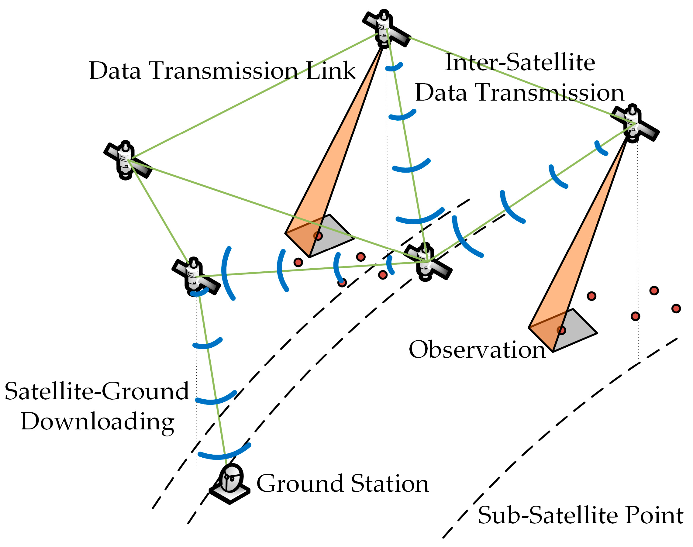
• The observation data can be temporarily saved in storage. During data transmission, there is no strict requirement to maintain continuous connectivity between all satellites. As shown in Figure 3, the generation of the data transmission path graph involves calculating inter-satellite data transmission time windows and determining if a data transmission path exists according to the data transmission time windows. In cases where satellites are not continuously connected (e.g., Satellite 1 and Satellite 3 in Figure 3), they can still be considered connectivity for data transmission if there is an inter-satellite data transmission time window between satellites;
• There can be multiple satellite nodes downloading data. It is necessary to identify the available satellites for downloading, find the optimal path for each download satellite, and pick the optimal solution among them;
• The distance between data transmission nodes will change with the data transmission mission arrangement.

Consequently, the conventional Dijkstra algorithm [28] is adapted to accommodate these specific requirements. The method of workflow is as follows:

• Based on the current observation solutions x_kiCur and g_ki,jCur, determine the observation result sequences s_k for each satellite, where $s_k=\left\{M_{k1},M_{k2},\dots ,M_{k{n}_{tk}}\right\}$, and n_tk is the number of observation targets for satellite k. Combine the observation result sequences of all satellites into one mission sequence $S=\left\{s_1,s_2,\dots ,s_{n_r}\right\}$;
• Calculate the satellite cluster’s status according to observation solutions and data transmission solutions related to missions that finished data transmission path planning;
• Select a mission M_ki in the mission sequence S by order. Take the satellite corresponding to the observation of mission M_ki as the starting satellite node l. Put the starting node into the selected node set ND_s, and put other satellite nodes into the unselected node set ND_u. Calculate the total distance d_l for the starting node. Initialize the total distance for the nodes in the unselected node and set ND_u to infinity. Set the starting node as the current node;
• Select the data transmission path planning strategy; the selection rules are described in Section 3.4.2. Calculate the inter-node distance a_l,lu between the current node l and all unselected nodes lu in the unselected node set ND_u based on the selected strategy. The calculation method for node distance is described in Section 3.4.3. Update d_lu according to the smaller value between d_l + a_{l, lu} and d_lu;
• Select the node l’ in the unselected node set N_Du with the smallest d_lu, and mark the current node l as the previous node of the node l’. Put l’ into the selected node set and delete it from the unselected node set. Set l’ as the current node l;
• Repeat steps 4–5 until there is no node left in the unselected node set;
• Record all the shortest paths corresponding to nodes that can download M_ki data. Sort recorded paths in ascending order based on the total distance d to the downloading nodes;
• Calculate the satellite cluster’s status and determine whether the constraints are satisfied for each recorded path by order. If a data transmission path satisfies the constraint, the mission can be transmitted through the path. Update solutions x_ki, y_ik,l, z_ikm, inter-satellite data transmission time, and satellite-ground data downloading time, and return to step 2. If no path satisfies the constraints, the observation solution does not satisfy the constraints and is considered infeasible, and the algorithm ends. If there are no remaining missions, the observation solution is feasible, the data transmission path planning for the corresponding observation solution is completed, and the algorithm ends.

3.4.2. State-Strategy Select Rules

In the Dijkstra algorithm, the total distance d determines how the next node is selected from the current node. In conventional routing algorithms, the inter-node distance a is calculated based on metrics such as transmission delay and remaining bandwidth. In the multi-satellite observation-relay transmission-downloading coupling scheduling problem, the objective function is the total profit of observation and downloading targets. During the data transmission path planning process, the choice of data transmission path affects the electric energy consumption, the occupancy of storage memory, and the occupancy of the satellite–ground data transmission time window, which in turn affects the number of observation and downloading targets, thus impacting the total value of observation and downloading targets. Specifically, when a mission completes the downloading to the ground earlier, more memory and a subsequent data transmission time window become available for transmitting data to other observation targets. Inter-satellite transmission consumes electrical energy, and if a mission completes data downloading by passing through more satellites for inter-satellite data transmission, it will consume more electrical energy for the entire satellite cluster. Based on the analysis, two strategies for calculating total distance d and inter-node distance a are proposed: one is the strategy of minimizing the data transmission node number, called the min-node strategy, and the other is the strategy of minimizing the data downloading start time, called the min-download time strategy. The calculation process is introduced below.

Firstly, the satellite-cluster state factors are calculated. The state factors of the satellite cluster include a data transmission state factor c_D and an electricity state factor c_E. Their formulas are described as

$$c_E={\psi }_E\min \frac{W_{k\min }}{P_{Camk}+\frac{P_{GroundDataTransk}{R}_{Camk}}{R_{GroundDataTransk}}+\Delta t_{AttitudeMissionk}{P}_{Attitudek}+c_{SolarConv}\left(\Delta t_{AttitudeMissionk}+\Delta t_o\right)P_{Ink}},$$

(21)

$$c_D=\begin{array}{cc}\min \left({\psi }_M\min \left(\frac{M_{Totalk}-M_{k\max }}{\Delta t_o{R}_{cam}}\right),{\psi }_D\min \left({\displaystyle \sum _{m=1}^{n_s}{\displaystyle \sum _{q=1}^{n_{dwkm}}\left(t_{dwekmq}-t_{dwskmq}\right)-{\displaystyle \sum _{i=1}^{n_t}{\displaystyle \sum _{m=1}^{n_s}\left(t_{dekmi}-t_{dskmi}\right)}}}}\right)\right)& z_{ikm}=1\end{array}.$$

(22)

In the equation of the electricity state factor c_E, W_kmin represents the minimum electric energy of satellite k during the scheduling period. The denominator of the fraction encompasses the total electric energy consumption for observation, data transmission, and attitude maneuvering for a single mission, where $\Delta t_{AttitudeMissionk}$ is the estimated attitude maneuver time for a single mission, and c_SolarConv represents the loss coefficient of solar array Power. ${\psi }_E$ represents the electricity influence coefficient. The electricity state factor c_E reflects the abundance of electric energy resources in the satellite cluster. For the data transmission state factor c_D, the left term indicates the abundance of memory in the satellite cluster, where M_kmax represents the maximum occupied memory of satellite k during the scheduling period, ${\psi }_M$ and ${\psi }_D$ represents the memory and data transmission time window influence coefficient. represents the electricity influence coefficient. The right term indicates the abundance of available satellite–ground transmission time in the satellite cluster. The data transmission state factor c_D reflects the abundance of both available memory and available satellite–ground transmission time in the satellite cluster.

Then the strategy is selected according to the selection rules:

IF c_E > c_D

THEN Rule = Rule_minTime

ELSE

THEN Rule = Rule_minNode

The rule signifies that when c_E is greater than c_D, it indicates that the satellite cluster’s memory resources and available satellite–ground data transmission time window are insufficient. Therefore, the selected strategy should prioritize the earliest data download time. Conversely, if the power supply is relatively limited, the strategy chosen should minimize the number of intermediary nodes, favoring the power supply subsystem.

3.4.3. Node Distance Calculation Method

In the process of calculating the inter-node distance a_k,l and the total distance d_k, several steps are involved. Firstly, the feasibility of inter-satellite data transmission between nodes and the feasibility of satellite–ground data transmission are determined. Then, the inter-satellite data transmission time and the satellite–ground data transmission time are calculated based on the data transmission feasibility. Finally, the inter-node distance a_k,l and the total distance d_k are calculated according to the chosen strategy.

Whether node k and node l are feasible for inter-satellite data transmission can be determined by calculating the data transmission available periods between the nodes. The inter-satellite data transmission time windows between node k and node l are $TR{W}_{kl}={\displaystyle \underset{p=1}{\overset{n_{rwkl}}{\cup }}\left[t_{rwsklp},t_{rweklp}\right]}$. The available period set TRA_kl between node k and node l is expressed as

$$TR{A}_{kl}=TR{W}_{kl}\cap T{M}_k\cap C_T\left(T{R}_{Ink}\cup T{R}_{Inl}\cup T{R}_{Outk}\cup T{R}_{Outl}\right),$$

(23)

where TM_k is the period after satellite k receives the data, which is expressed as

$$T{M}_k=\{\begin{array}{cc}\left[t_{oeki},t_e\right]& x_{ki}=1\\ \left[t_{rInelki},t_e\right]& y_{il,k}=1\end{array},$$

(24)

where $C_T\left(T{R}_{Ink}\cup T{R}_{Inl}\cup T{R}_{Outk}\cup T{R}_{Outl}\right)$ are the available time segments excluding current inter-satellite data transmission mission periods, where T is the total scheduling period, and $T{R}_{Ink}$, $T{R}_{Inl}$, $T{R}_{Outk}$, $T{R}_{Outl}$ represent the current data transmission mission period segments of satellites k and l. tra_kl is a single period in the period set TRA_kl. The condition for inter-satellite data transmission between nodes k and l is that there should be at least one time period tra_kl has enough time for a data transmission mission. If the data transmission condition between nodes k and l is satisfied, mark Flag_rikl = 1, otherwise Flag_rikl = 0.

Whether node k is feasible for satellite–ground data downloading to ground station m can be determined by calculating the available downloading periods. The available period set TDA_km between node k and stations is expressed as

$$TD{A}_{km}=TD{W}_{km}\cap T{M}_k\cap C_T\left(T{D}_k\right),$$

(25)

where $TD{W}_{km}={\displaystyle \underset{m=1}{\overset{n_s}{\cup }}{\displaystyle \underset{q=1}{\overset{n_{dwkm}}{\cup }}\left[T_{dwskmq},T_{dwekmq}\right]}}$ are the satellite–ground data transmission time windows between node k and ground station m. The description of TM_km is the same as the description in the inter-satellite data transmission available time calculation. TD_k represents the current data downloading mission period segments of node k. tda_km is a single period in the period set TDA_km. The condition for satellite–ground data downloading at node k is that there should be at least one time period during which tda_km has enough time for the data downloading mission. If the data downloading condition of node k is satisfied, mark Flag_gik = 1, otherwise Flag_gik = 0. The data-downloading mission. The downloading start time of satellite k to mission i is arranged at the minimum start time of all available periods, which is denoted as $t_{dsik{m}_{\min }}$, m_min is the ground station index corresponding to the minimum start time of all available periods.

In the Dijkstra algorithm for calculating total distance d_lu and inter-node distance a_l,lu from node l to node lu. The calculation of total distance d_lu while using the min-node strategy is described as

$$d_{lu}=\{\begin{array}{cc}{n}_{Passlu}& Fla{g}_{gilu}=1\\ \inf & Fla{g}_{gilu}=0\end{array},$$

(26)

where n_Passlu is the number of relay satellites. The calculation while using the min-download time strategy is described as

$$d_{lu}=\{\begin{array}{cc}{t}_{dsilu{m}_{\min }}/\left(t_e-t_s\right)& Fla{g}_{gilu}=1,Fla{g}_{rillu}=1\\ t_e-t_s+t_{rOutsl{l}_u}/\left(t_e-t_s\right)& Fla{g}_{gilu}=0,Fla{g}_{rillu}=1\\ \inf & Fla{g}_{rillu}=0\end{array}.$$

(27)

For two strategies, the calculation of inter-node distance a_l,lu is expressed as

$$a_{l,lu}=\{\begin{array}{cc}{d}_{lu}-d_l& Fla{g}_{rillu}=1\\ \inf & Fla{g}_{rillu}=0\end{array}.$$

(28)

After calculating the total distance d and the inter-node distance a, the path selection can be performed according to the Dijkstra algorithm.

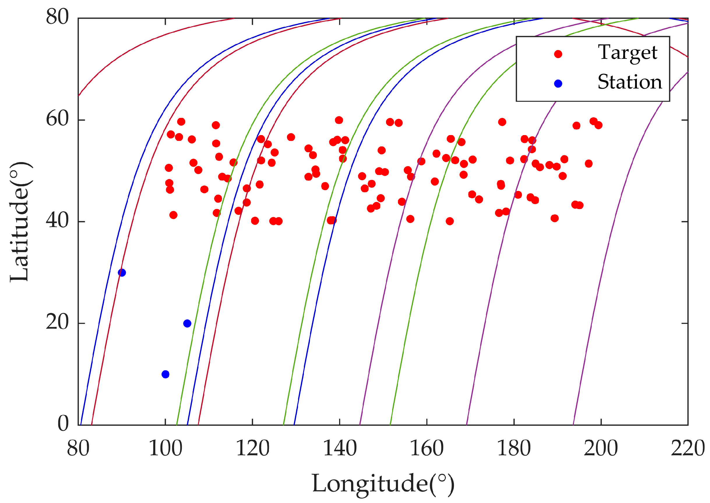
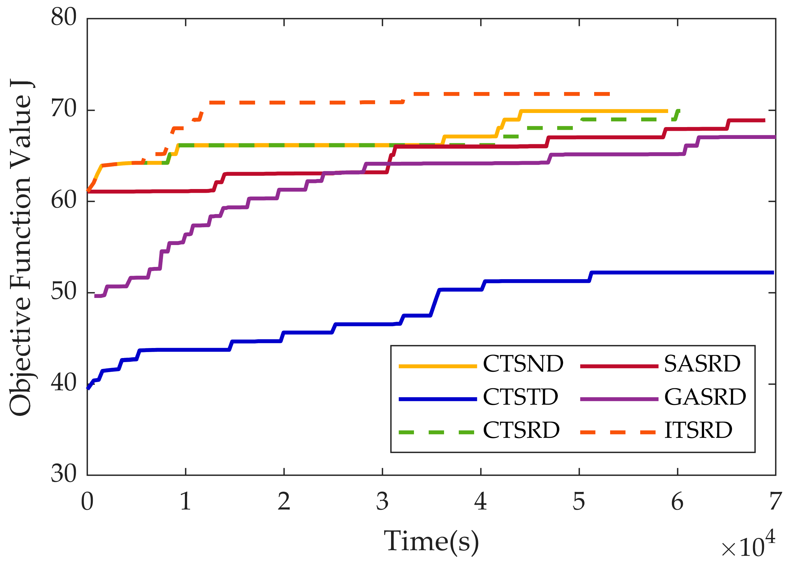
4. Simulation Results

Two scenarios were constructed to verify the improvement of the local search process in tabu search and the improvement of the data transmission path planning method. In the design of the simulation scenarios, the selected target points are time periods other than the orbital periods of the satellite–ground data transmission time window. In this kind of scenario, due to the limitation of storage capacity caused by the failure to download the observation data in time, the traditional scheduling methods of multi-satellite observation and single-satellite downloading will limit the number of targets observed by the satellite cluster. In contrast, by applying the multi-satellite observation-relay transmission-download coupling scheduling method, the observation data can be transmitted in time through inter-satellite data transmission, so that the satellite has more available storage capacity to observe other targets, which can maximize the observation ability and improve the observation profit of the whole satellite cluster.

For the improvement of data transmission path planning, the local search method of the tabu search algorithm was kept as the conventional local search method, and we compared the improved method of transmission planning with the two conventional methods. The data transmission path planning method in the improved method is the rule-based data transmission path planning method proposed in this article. The name of the complete method is the conventional tabu search-rule-based Dijkstra data transmission path planning method (CTSRD). The data transmission path planning method used in the improved method is the strategy-based Dijkstra method [28], adapted to the problem in this article. The strategies are the min-node strategy and min-download time strategy proposed in this article. The names of the complete methods are conventional tabu search-min-node Dijkstra data transmission path planning method (CTSND) and conventional tabu search-min-download time Dijkstra data transmission path planning method (CTSTD).

For the improvement of the local search process in Tabu Search, the data transmission path planning method was kept as the improved rule-based Dijkstra data transmission path planning method, and we compared the improved local search process in Tabu Search proposed in this article with the conventional Tabu Search [45]. The name of the complete method corresponding to the improved local search process is the improved tabu search-rule-based Dijkstra data transmission path planning method (ITSRD).

Meanwhile, two other meta-heuristic methods were added to the simulation, including the simulated annealing algorithm [56] and the genetic algorithm [57]. The data transmission path planning method in this article was added to the simulated annealing algorithm and the genetic algorithm to solve the multi-satellite observation-relay transmission-download coupling scheduling problem. The names of these methods after adaptive transformation are SASRD and GASRD. The neighborhood construction method of SASRD adopts the neighborhood construction method in this article. In the SASRD parameters setting, the initial temperature was set to 1, the temperature decreasing rate was set to 0.95, and the ending temperature was set to 1 × 10⁻⁶. The population size of GASRD was 100, the crossover probability was 0.6, and the mutation probability was 0.4.

The setting rules for parameters in the scheduling method are as follows: W_warning is the warning value of satellite-available electric energy, which is set based on the electric energy required for observation and downloading to accomplish a single observation mission. When the available electric energy of a satellite is less than W_warning, the satellite cannot finish the complete observation and downloading process of a single mission. At this moment, the solution can hardly be further improved, the search process can easily fall into the local optimal state, and the search direction needs to be adjusted. In this article, $W_{Warning}=20\times 1000+40\times 500=4\times {10}^4$. $\Delta t_{DWarning}$ is the warning value of the available time for data downloading. It can be determined according to the downloading time required for the target observation data. When the available data transmission time to the ground is less than this value, the satellite cannot carry out more observations, and the search process can easily fall into the local optimal state. In this article, $\Delta t_{DWarning}=20\times 1000/500=40$. The $\Delta t_{AttitudeMissionk}$ is the attitude maneuver time estimated value of a single target observation. It is set according to the average value of the attitude maneuver time of a single target observation. According to the attitude maneuver ability of the satellite in this article, it was set to 20. $c_{SolarConv}$ is the conversion coefficient of solar array charging power efficiency reduction caused by satellite orbit motion and attitude maneuver. According to the satellite orbit and attitude maneuver parameters in this paper, it was set to 0.5. ${\xi }_W$ is the electric reward weight of local search improvement. This parameter helps the electricity–benefit solution rank higher among solutions. The parameter is set based on the profit of a single target observation in the scenario. Considering the extra electric energy consumption of inter-satellite data transmission, this parameter can be appropriately increased. ${\xi }_W$ was set to 1 in this article. ${\xi }_D$ is the data transmission reward weight of local search improvement. This parameter helps the data transmission-benefit solution rank higher among solutions. The parameter is set based on the profit of a single target observation in the scenario. ${\xi }_D$ was set to 0.6 in this article. The values of ${\psi }_E$, ${\psi }_D$ and ${\psi }_M$ are determined by the influence of different parameter values on the scheduling results under typical conditions. Since the choice of data transmission path planning strategy is selected by the comparison of c_D and c_E, the parameter value of ${\psi }_E$, ${\psi }_D$ and ${\psi }_M$ can be determined by the adjustment of ${\psi }_D$ and ${\psi }_M$ while keeping ${\psi }_E$ unchanged. In this article, ${\psi }_E$ was set to 1. When the value of ${\psi }_D$ were 1, 2, 3, under the typical condition of scenario 1, the optimal objective function values were the same value as 71.78. Under the typical condition of scenario 2, the optimal objective function values are the same value as 64.56. When the values of ${\psi }_M$ were 1, 2, 3, under the typical condition of scenario 1, the optimal solution objection function values are 70.8, 71.8, and 71.8. Under the typical condition of scenario 2, the scheduling result and the iterations to reach the optimal solution have the same value of 64.56. Therefore, the value change of ${\psi }_D$ in this article has little effect on the scheduling results. ${\psi }_D$ was set to 1 and ${\psi }_M$ was set to 2.

In summary, the method parameters set in the article were ${\xi }_W=1$, ${\xi }_D=0.6$, $W_{Warning}=4\times {10}^4$, $\Delta t_{DWarning}=40$, ${\psi }_E=1$, ${\psi }_D=1$, ${\psi }_M=2$, $\Delta t_{AttitudeMissionk}=20$, $c_{SolarConv}=0.5$. The scheduling period was 15,000 s. The calculation program was executed on a computer with an Intel Core i7-8700@3.2 GHz CPU. The maximum number of iterations was set at 200. The satellite parameters used in the simulation were configured based on the reference [58], as given in Tables 3 and 6.

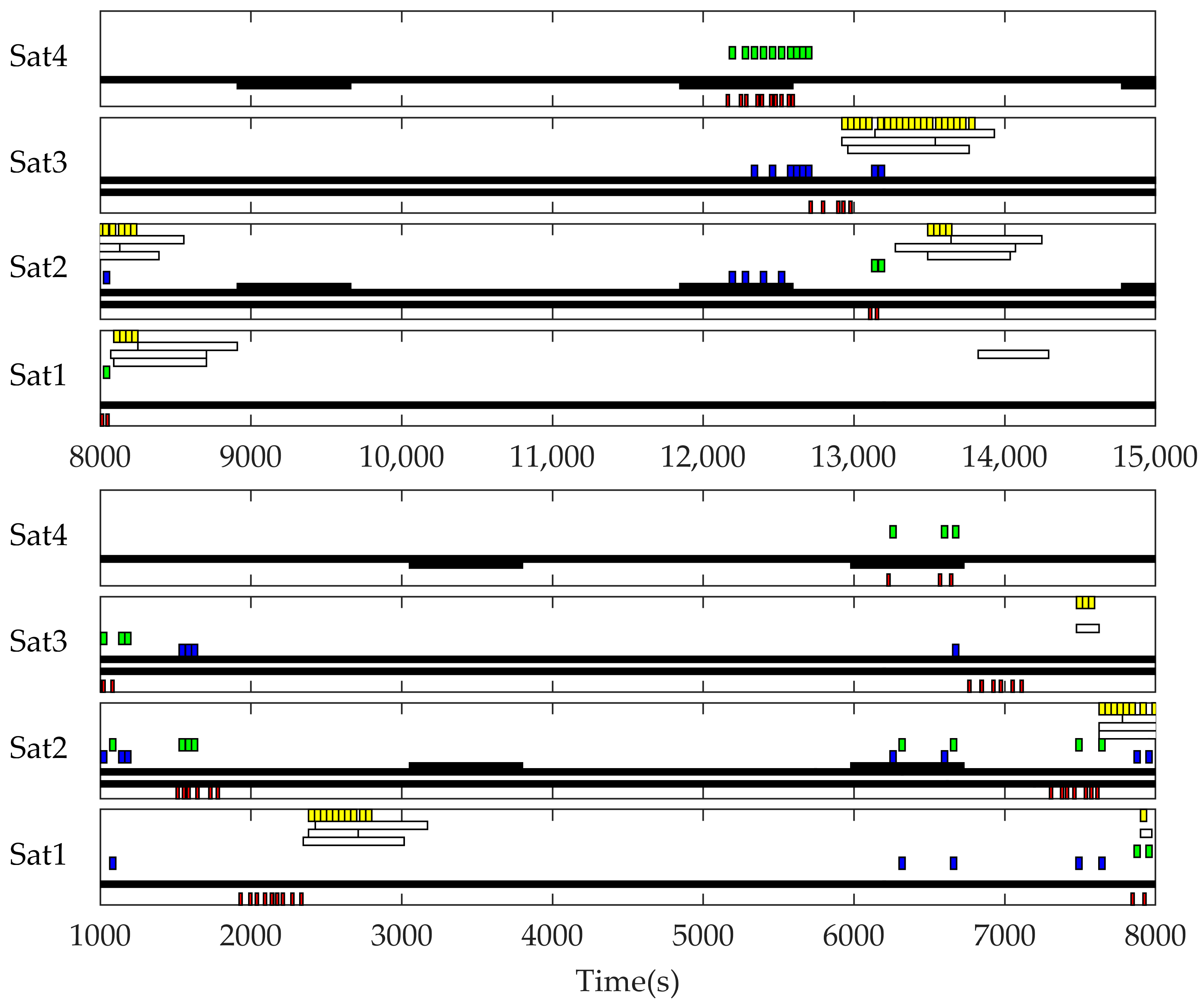
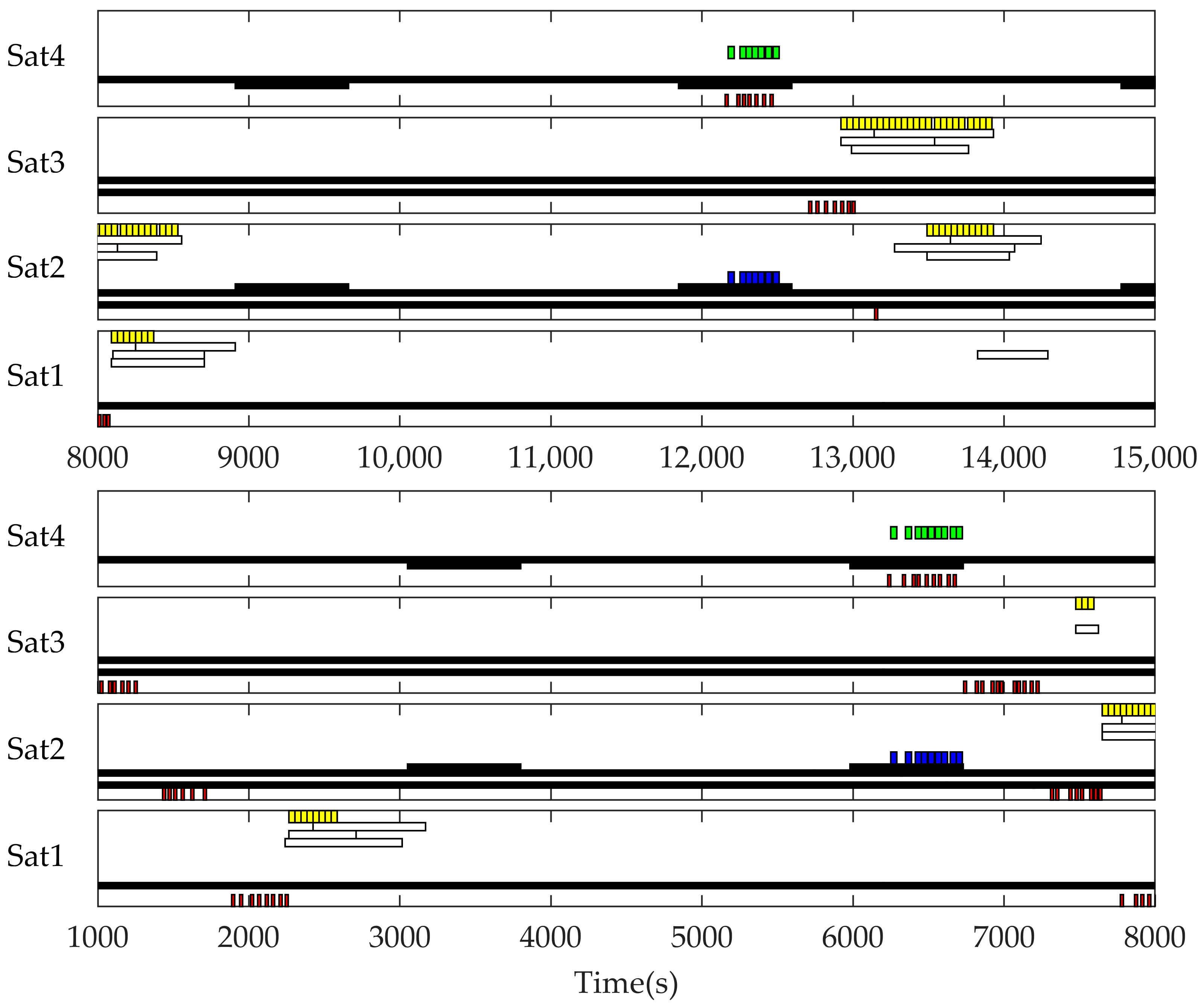
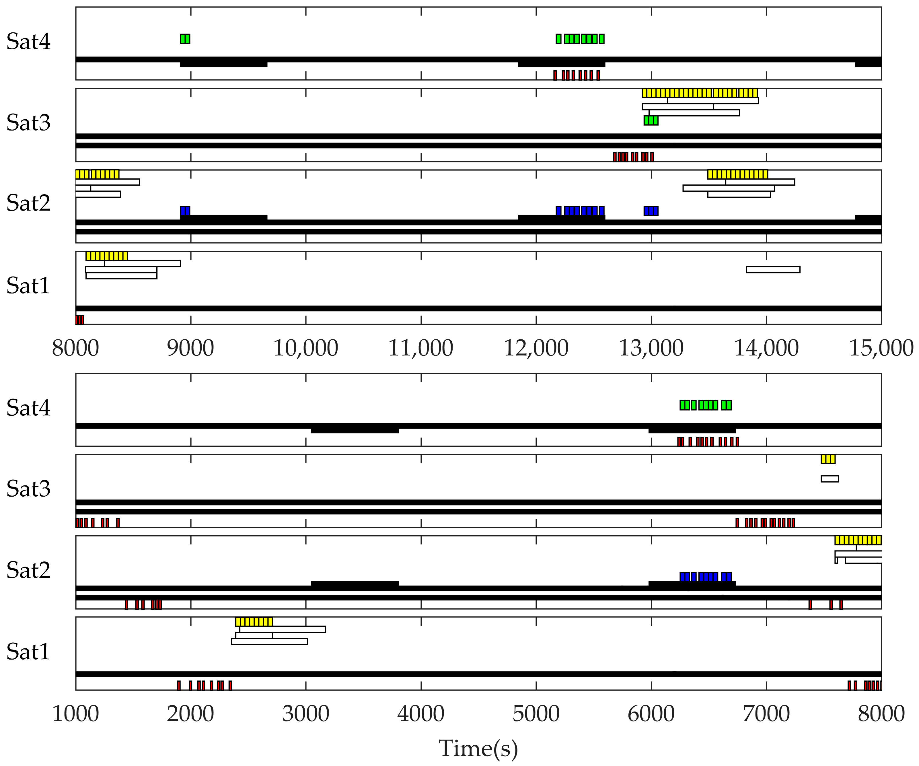
4.1. Scenario 1 Insufficient Electric Energy Scenario

Scenario 1 represented an insufficient electric energy scenario where the satellites had limited initial power. There were four satellites with sun-synchronous orbits. The orbital parameters of the satellites are shown in

Table 2. Initial satellites orbit parameters in scenario 1.

Satellite No	Semi-Major Axis (m)	Eccentricity	Inclination (°)	RAAN (°)	Argument of Perigee (°)	True Anomaly (°)
1	7,028,140	0	97.9908	40.348	0	0
2	7,028,140	0	97.9908	80.348	0	30
3	7,028,140	0	97.9908	120.348	0	60
4	7,028,140	0	97.9908	160.348	0	90

. The subsystem parameters of the four satellites were the same, as shown in

Table 3. Satellite subsystem parameters in scenario 1.

Parameter Name	Parameter Value
Attitude Maneuver Calculate Method	Trapezoidal Method
Max Attitude Maneuver Angular Velocity	1°/s
Max Attitude Maneuver Angular Acceleration	0.5°/s2
Max Maneuvering Range Half-Cone Angle	45°
Antenna Coverage Half-Cone Angle	70°
Storage Capacity	1000 Gbit
Camera’s Data Generation Rate	2 Gbps
Satellite-Satellite Data Transmission Rate	1 Gbps
Satellite-Ground Station Data Transmission Rate	1 Gbps
Battery Electrical Energy Capacity	5 × 106 J
Battery Initial Electrical Energy	1 × 106 J
Max Charging Electrical Power of Solar Arrays	1 kW
Camera Electrical Power	1 kW
Satellite-Satellite Data Transmission Devices Electrical Power	0.5 kW
Satellite-Ground Station Data Transmission Devices Electrical Power	0.5 kW
Satellite Attitude Maneuver Electrical Power	0.2 kW
Satellite Normal Electrical Power	0.55 kW
Observation time of a single target	20 s

.

In this scenario, five conditions are generated by randomly generating target points. The improvement effect of the method in this article is explained by the statistical results comparison of each method in multiple conditions and the results comparison of each method in a single condition. The target number was set to 100 in this scenario; the longitude ranges were [100°, 180°] and [−180°, −160°], and the latitude range was [40°, 60°]. The scenario included 3 ground stations with the following coordinates: (105°, 20°), (90°, 30°), and (100°, 10°). The profit from the target points was randomly assigned between 0.9 and 1. The distribution of targets and ground stations is shown in Figure 4.

The statistical results of the comparison of all six methods are shown in

Table 4. Statistical results of different methods in scenario 1.

	Optimal Solution Objective Function Value			Optimal Solution Iteration Time (s)
Method	Max	Min	Average	Max	Min	Average
CTSND	73.06	67.70	70.56	53,449.45	43,823.98	47,950.01
CTSTD	61.52	52.24	56.68	62,552.34	29,555.25	48,103.63
CTSRD 1	73.06	67.70	70.20	60,007.70	36,706.24	47,109.22
SASRD	72.87	64.82	68.59	68,923.34	51,544.14	61,194.55
GASRD	69.81	63.58	67.13	77,119.22	56,474.78	64,570.52
ITSRD 2	74.80	69.45	72.88	40,172.14	22,252.50	32,140.57

¹ Verifying the improvement of data transmission path planning. ² Verifying the improvement of the local search process and data transmission path planning.

. The average optimal solution objective function values and the average optimal solution iteration time of each method are compared as follows: The optimal solution objective function values of CTSRD and CTSND are nearly the same. The optimal solution objective function value of CTSRD is 23.9% higher than that of the initial solution of CTSTD. The optimal solution iteration times of CTSND, CTSTD, and CTSRD are nearly the same. The optimal solution objective function value of ITSRD is 3.8% higher than that of CTSRD, and the time required for ITSRD to reach the optimal solution is 31.8% less than that of CTSRD. The optimal solution objective function values of SASRD and GASRD are slightly lower than those of CTSRD, and it takes longer to reach the optimal solution. ITSRD performs better than SASRD and GASRD in terms of the optimal solution objective function value and the optimal solution iteration time.

Figure 5 presents the iterative results of different methods in a single condition of scenario 1. The comparison between the orange dashed line and the green dashed line in the figure illustrates the impact of the improvement in tabu search. The improved tabu search method escaped from the local optimum and searched toward a more optimal solution after 15 iterations. In contrast, the traditional tabu search method did not escape from the local optimum until 143 iterations. The final result of the improved tabu search method was also better than the traditional tabu search method. It can be seen from the figure that the solutions of SASRD and GASRD are continuously improved, which reflects that SASRD and GASRD have global search ability and potential. However, due to the length of time of the single-step solutions, SASRD and GASRD need more time to achieve optimal solutions.

Figure 6, Figure 7 and Figure 8 show the observation and data transmission event diagram of different methods: the red strips are the observation period, the green strips are the inter-satellite output data transmission period, the blue strips are the inter-satellite input data transmission period, the yellow strips are the satellite–ground data transmission period, the black strips are the inter-satellite data transmission time window, and the white strips are the ground data transmission time window. The timing relationship between the observation periods, the inter-satellite data transmission periods, and the satellite–ground data transmission periods in the figures shows that the multi-satellite observation-relay transmission-download coupling scheduling method can realize the whole process of scheduling multi-satellite observation, relay transmission, and downloading.

It can be seen from the number of blue and green strips in Figure 6 and Figure 7 that CTSRD performed less inter-satellite data transmission than CTSTD, so more electric energy could be used for target observation and data transmission of CTSRD and more missions could be completed, thus the objective function value was better. For the insufficient electric energy on satellites 1 and 2, ITSRD performed fewer observation missions than CTSRD, reducing the consumption of attitude maneuver electric energy to complete more inter-satellite data transmission missions and satellite-download data transmission missions, thus the objective function value was better. This shows that the improved tabu search algorithm helps the satellite cluster observe more targets by adjusting the state of the satellite electricity subsystem and indicates the improvement of using the subsystem coupling relationship to help the search method escape from the local optimum.

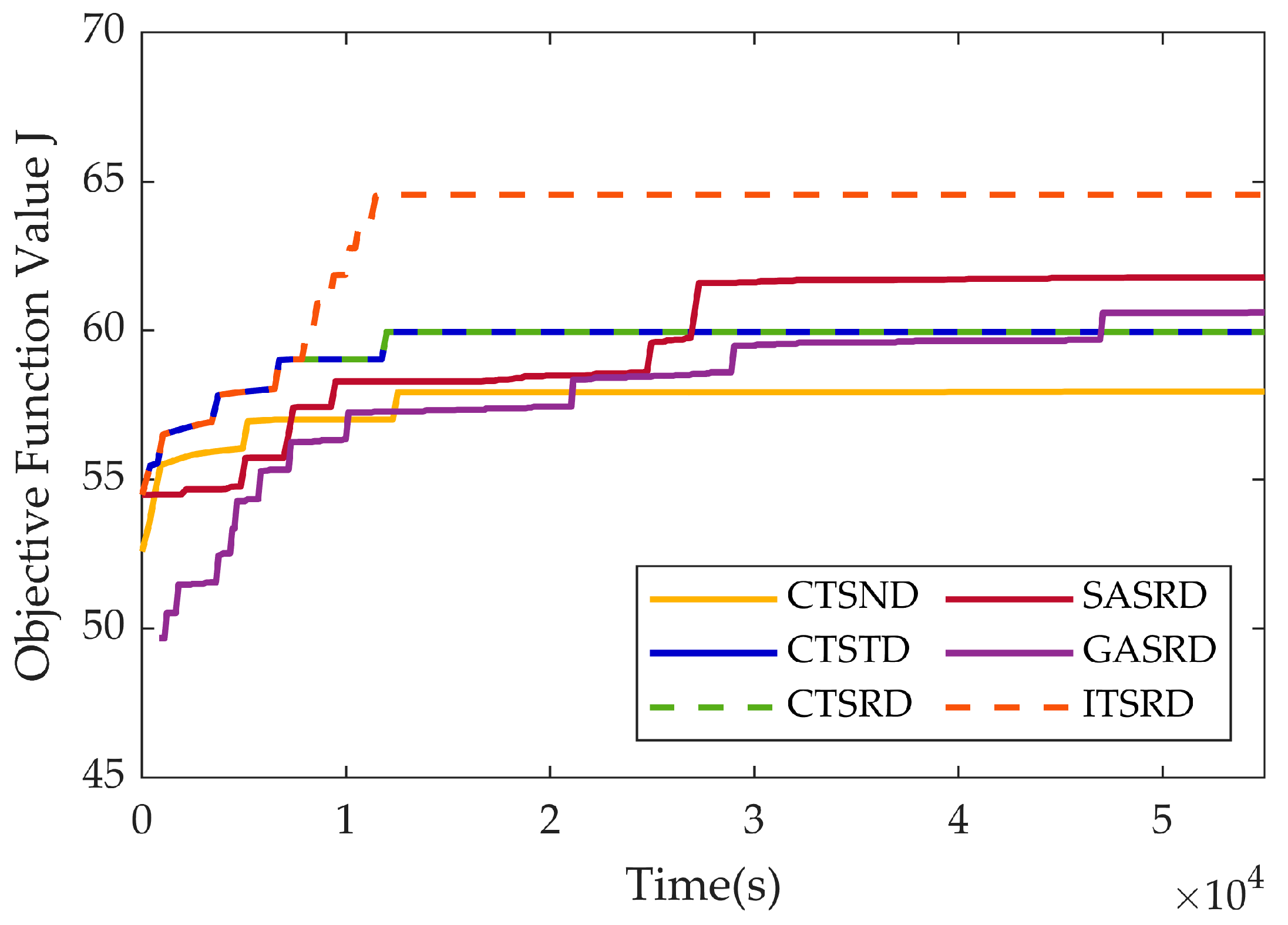
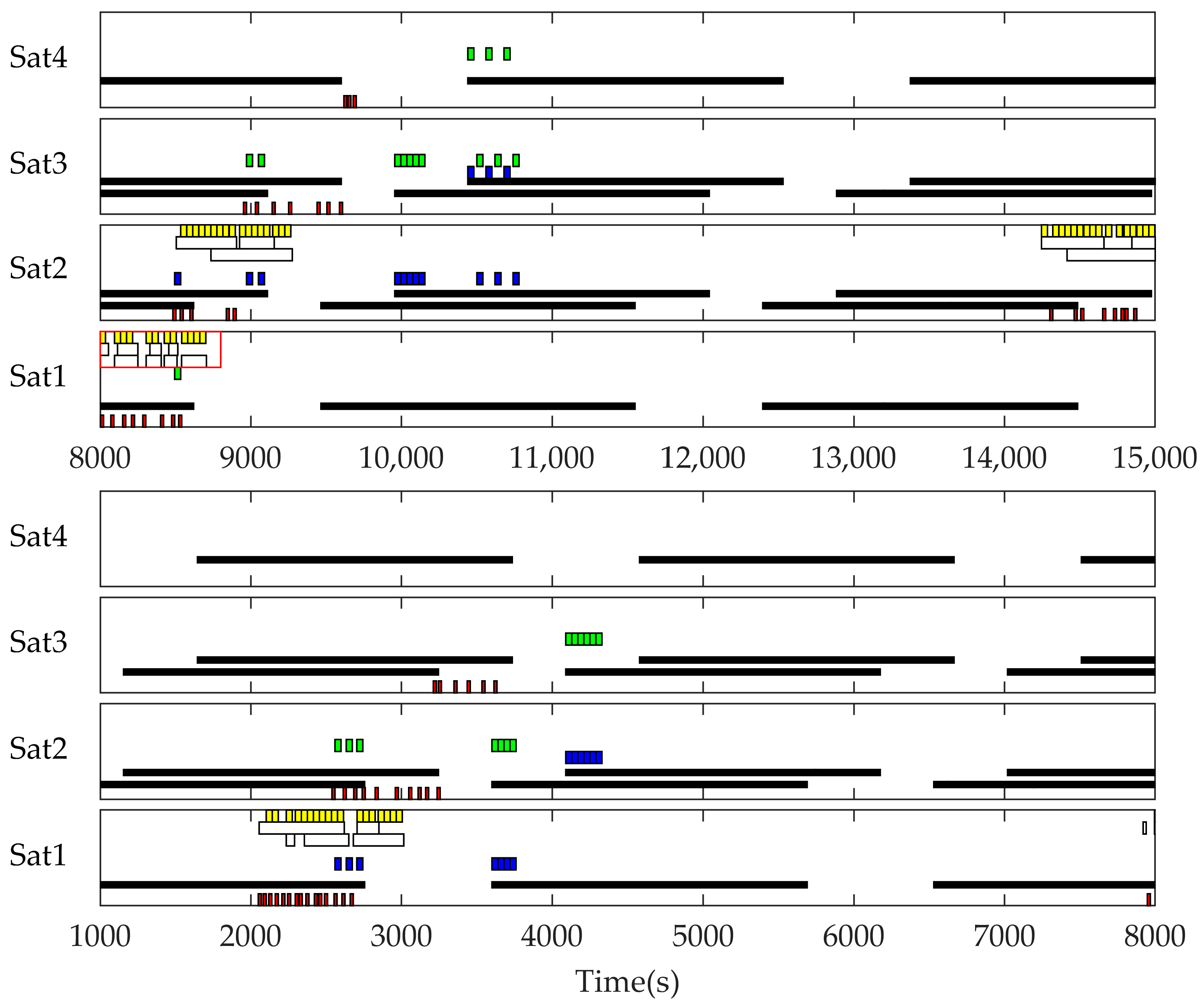
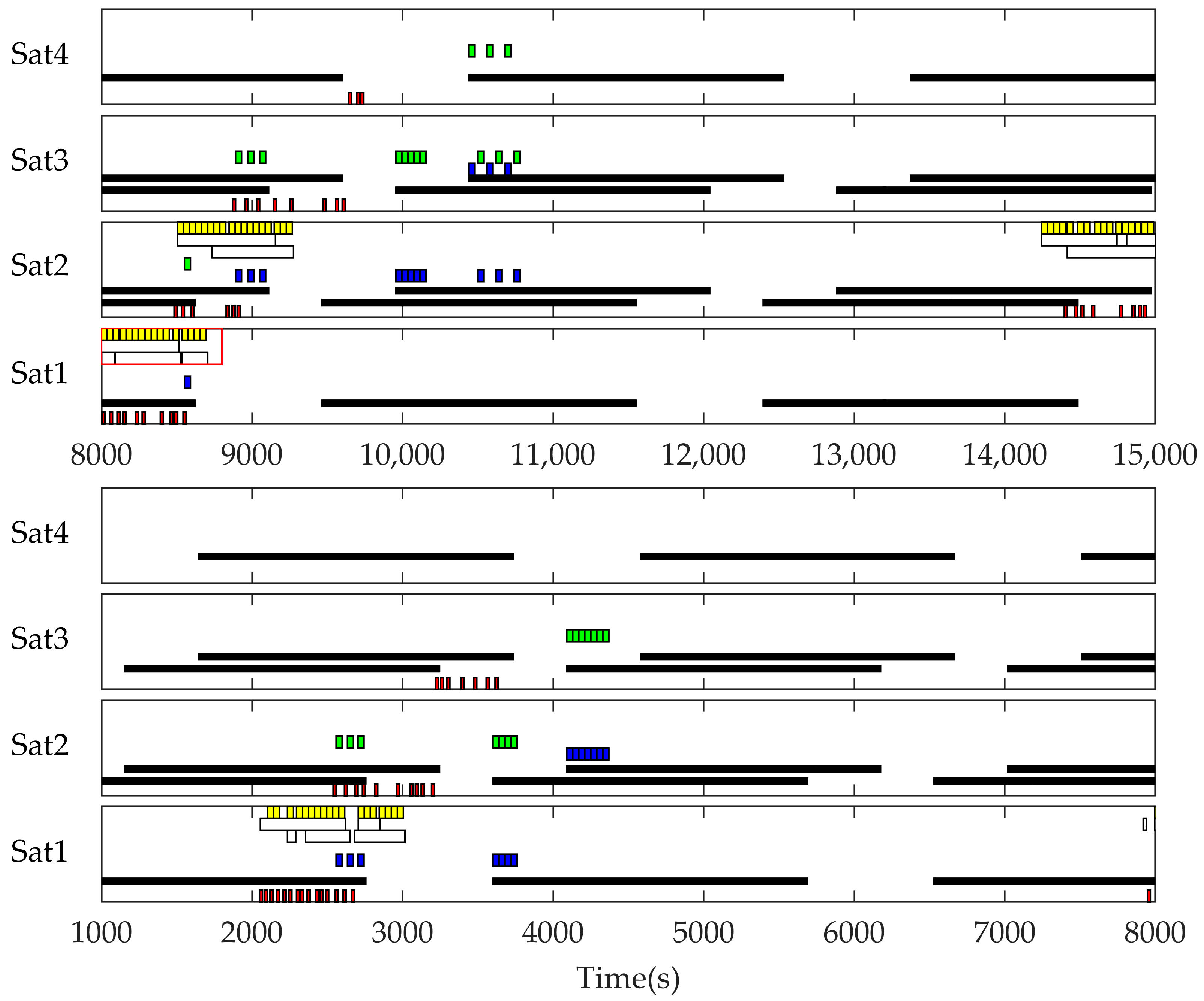
4.2. Scenario 2 Insufficient Data Transmission Resource Scenario

Scenario 2 represented an insufficient data transmission resource scenario where the satellites have limited memory capacity and limited satellite–ground data transmission time windows. There were four satellites with sun-synchronous orbits. The orbital parameters of the satellites are shown in

Table 5. Initial satellite orbit parameters in Scenario 2.

Satellite No	Semi-Major Axis (m)	Eccentricity	Inclination (°)	RAAN (°)	Argument of Perigee (°)	True Anomaly (°)
1	7,028,140	0	97.9908	40.348	0	0
2	7,028,140	0	97.9908	80.348	0	−30
3	7,028,140	0	97.9908	120.348	0	−60
4	7,028,140	0	97.9908	160.348	0	−90

. The subsystem parameters of the four satellites were the same, as shown in

Table 6. Satellite subsystem parameters in Scenario 2.

Parameter Name	Parameter Value
Attitude Maneuver Calculate Method	Trapezoidal Method
Max Attitude Maneuver Angular Velocity	1°/s
Max Attitude Maneuver Angular Acceleration	0.5°/s2
Max Maneuvering Range Half-Cone Angle	45°
Antenna Coverage Half-Cone Angle	70°
Storage Capacity	500 Gbit
Camera’s Data Generation Rate	2 Gbps
Satellite-Satellite Data Transmission Rate	1 Gbps
Satellite-Ground Station Data Transmission Rate	1 Gbps
Battery Electrical Energy Capacity	5 × 106 J
Battery Initial Electrical Energy	5 × 106 J
Max Charging Electrical Power of Solar Arrays	1 kW
Camera Electrical Power	1 kW
Satellite-Satellite Data Transmission Devices Electrical Power	0.5 kW
Satellite-Ground Station Data Transmission Devices Electrical Power	0.5 kW
Satellite Attitude Maneuver Electrical Power	0.2 kW
Satellite Normal Electrical Power	0.55 kW
Observation time of a single target	20 s

.

In this scenario, five conditions are generated by randomly generating target points. The improvement effect of the proposed method in this article is explained by the statistical results comparison of each method in multiple conditions and the results comparison of each method in a single condition. The target number was set to 150. In this scenario, the longitude ranges were [80°, 180°] and [−180°, −160°], and the latitude range was [10°, 50°]. The scenario included 2 ground stations with the following coordinates: (105°, 20°), (110°, 30°). The profit from the target points was randomly assigned between 0.9 and 1. The distribution of targets and ground stations is shown in Figure 9.

The statistical results of the comparison of all six methods are shown in

Table 7. Statistical results of different methods in scenario 2.

	Optimal Solution Objective Function Value			Optimal Solution Iteration Time(s)
Method	Max	Min	Average	Max	Min	Average
CTSND	60.19	55.31	58.03	47,471.11	32,533.38	42,458.55
CTSTD	64.87	59.21	61.52	52,480.11	11,987.33	39,925.27
CTSRD 1	64.87	59.21	61.52	52,510.30	11,987.42	39,951.82
SASRD	64.75	59.28	61.99	56,374.09	40,695.00	49,539.53
GASRD	65.64	59.46	62.37	68,194.30	49,960.36	61,536.70
ITSRD 2	67.67	63.20	64.86	51,163.97	11,726.50	30,114.90

¹ Verifying the improvement of data transmission path planning. ² Verifying the improvement of the local search process and data transmission path planning.

. The average optimal solution objective function values and the average optimal solution iteration time of each method are compared as follows: The optimal solution objective function values and the optimal solution iteration time of CTSRD and CTSTD are nearly the same. The optimal solution objective function value of CTSRD is 6% higher than that of CTSND. The optimal solution iteration time of CTSRD is 5.9% less than that of CTSND. The optimal solution objective function value of ITSRD is 5.4% higher than that of CTSRD, and the time required for ITSRD to reach the optimal solution is 24.6% less than that of CTSRD. The optimal solution objective function values of SASRD and GASRD are slightly higher than those of CTSRD, but it takes longer to reach the optimal solution. ITSRD performs better than SASRD and GASRD in terms of the optimal solution objective function value and the optimal solution iteration time.

Figure 10 presents the iterative results of different methods. The comparison between the orange dashed line and the green dashed line in the figure illustrates the impact of the improvement in tabu search. It can be seen from the figure that, before 26 iterations, the search process of the two methods was the same. After 26 iterations, the traditional tabu search method falls into the local optimum; when reaching 39 iterations, it has been improved, but the improvement is limited. In contrast, the improved tabu search method escapes from the local optimum and continues to search in the direction of a better solution, which reflects that the improved tabu search method improves the ability to escape from the local optimum. The scheduling results of SASRD and GASRD are better than those of the traditional tabu search algorithm, but it takes longer to reach the optimal solution.

It can be seen from the red boxes in Figure 11 and Figure 12 that ITSRD had more satellite–ground data transmission periods than CTSRD to complete more satellite–ground data downloading missions in the insufficient data transmission resource scenario, resulting in a better objective function value. It can be implied that the traditional tabu search method can easily fall into the local optimum due to the complexity of the subsystem coupling scheduling of the multi-satellite observation-relay transmission-download coupling scheduling problem. Additionally, by adjusting the data transmission time windows, the improved tabu search method can assist the satellite in transmitting more observation data. Hence, the objective function value is improved, which implies that the improved tabu search method is able to prevent the search method from falling into the local optimum by adjusting the states of the satellite cluster subsystem.

5. Discussion

From the event flowcharts of the simulation results, it is shown that by incorporating the data transmission path planning method into the observation scheduling method, the entire process of coupling the scheduling of observation, relay transmission, and downloading can be achieved. This process enables the observation satellite to download the data through other satellites relaying in the non-data transmission window orbit period to reduce the storage occupation, so that the satellite has more available storage capacity to complete other target observations and improves the observation ability of the satellite cluster.

The statistical simulation results reveal that, in the scenario of insufficient electric energy, the average optimal solution objective function values of CTSRD and CTSND are nearly the same. The average optimal solution objective function value of CTSRD is 23.9% higher than that of CTSTD. The average optimal solution iteration time of CTSND, CTSTD, and CTSRD is nearly the same. In the simulation scenario of insufficient data transmission resources, the average objective function values of the optimal solutions of CTSRD and CTSTD are the same, and the time to reach the optimal solution is nearly the same. The average optimal solution objective function value of CTSRD is 6% higher than that of CTSND, and the iteration time to reach the optimal solution of CTSRD is 5.9% less than that of CTSND. The comparison among different methods of data transmission path planning shows that the proposed rule-based Dijkstra data transmission planning method has better adaptability in different conditions of satellite cluster states and environments. At the same time, it also shows that the two Dijkstra planning methods based on strategies are effective only in the corresponding conditions.

In the scenario of insufficient electric energy, the average optimal solution objective function value of ITSRD is 3.8% higher than that of CTSRD, and the average time required to reach the optimal solution of ITSRD is 31.8% less than that of CTSRD. In the scenario of insufficient data transmission resources, the average optimal solution objective function value of ITSRD is 5.4% higher than that of CTSRD, and the average time required for ITSRD to reach the optimal solution is 24.6% less than that of CTSRD. The result comparisons between ITSRD and CTSRD show that the improved local search process in tabu search improves the searching efficiency. In the two scenarios, ITSRD achieves the best optimal solution and the shortest iteration time for reaching the optimal solution of all methods, which also reflects the improvement effect of the method proposed in this article.

In the multi-satellite observation-relay transmission-download coupling scheduling problem, the improved tabu search method in this article outperforms the conventional simulated annealing algorithm and the genetic algorithm in terms of calculation results and calculation time. As compared with the traditional tabu search algorithm, the simulated annealing algorithm and the genetic algorithm reflect the ability and potential of global search, but it takes a longer time to reach the optimal solution. As a consequence of the complexity of the working process and multi-subsystem constraints, it takes more time to calculate the constraint satisfaction of a single solution, which leads to more time consumption in each iteration for each iteration, resulting in an increase in the search time of the entire search method. The search results of the simulated annealing algorithm reflect the uncertainty of the solution caused by the random search process. In order to improve the stability of the results and obtain better outcomes, it is necessary to further reduce the temperature-decreasing rate and increase the number of iterations, which results in an additional rise in calculation time. In the genetic algorithm searching process, due to the multi-subsystem constraints, the generated solutions contain lots of unwanted solutions in a single-step iteration process. It is necessary to adjust the solution to meet the constraints. In this way, it will take more time in the single-step calculation, thus reducing the overall solution efficiency.

In the iterative results comparison diagram of the two simulation scenarios, it is apparent that the improved tabu search method and the traditional tabu search method maintain the same search effect at the initial stage of the search. When the traditional tabu search method falls into the local optimum, the improved tabu search method shows the ability to escape from the local optimum. Through the analysis of the observation and data transmission event diagram, it is clear that the reason why the traditional tabu search algorithm falls into the local optimum is due to the coupling constraints of the electricity subsystem and the data transmission subsystem. The improved tabu search algorithm also gives the satellite the ability to observe and transmit more target data by adjusting the state of the satellite cluster subsystems and also to escape the local optimum, which justifies the viewpoint of the improved tabu search method in this article.

This research can be further extended in the following aspects:

• The global–local combination methods are also an important development direction for search methods. Combining the advantages of global search methods and local search methods, the multi-satellite observation-relay transmission-downloading coupling scheduling method can be improved;
• Further research can be carried out under different target distributions, ground station distributions, and satellite parameters. Finding out the influence of the parameters of the method on the results under different scenarios. The relationship between the parameters of the algorithm and the adaptive working conditions is explored using system analysis and machine learning in order to enhance the adaptability of the method under different working conditions. In addition, mining the relationship between the parameters of the algorithm and the adaptive scenarios by using system analysis and machine learning methods can enhance the adaptability of the scheduling method in different scenarios.
• Study the scheduling method with a large-scale satellite cluster and a large number of targets so as to alleviate the trade-off between calculation results and calculation efficiency in large-scale problems.
• In the case of increasing data transmission, how to transmit data to the ground station stably and quickly in the conditions of large data transmission volumes and communication interference is also one of our future research directions.

6. Conclusions

In this article, an improved tabu search method for the multi-satellite observation-relay transmission-downloading coupling scheduling problem is proposed. Based on the multi-satellite earth observation tabu search algorithm, the data transmission path planning method for observation data transmission and downloading planning is introduced. The satellite observation scheduling tabu search algorithm is improved, referring to the idea of the artificial potential field method. Additionally, in the data transmission path planning method, two strategy methods, including the “min-node strategy” and the “min-download time strategy”, are proposed based on the Dijkstra data transmission path planning method. Based on the strategy Dijkstra method, the state-strategy selection rules are introduced, and the rule-based Dijkstra data transmission path planning method is proposed. The simulation results show that the proposed entire process coupling scheduling method can schedule the observation, relay transmission, and download processes of the satellite group, and the achievement of the entire process scheduling enhances the ability of the satellite cluster to obtain the observation data. The improved Dijkstra method enhances adaptability to the multi-subsystem coupled problem, and the improved local search in the tabu search method amplifies the algorithm’s search capability.

References

1. Gu, X.F.; Tong, X.D. Overview of China Earth Observation Satellite Programs. IEEE Geosci. Remote Sens. Mag. 2015, 3, 113–129. [Google Scholar] [CrossRef]
2. Gleyzes, M.A.; Perret, L.; Kubik, P. Pleiades System Architecture and Main Performances. In Proceedings of the 22nd Congress of the International-Society-for-Photogrammetry-and-Remote-Sensing, Melbourne, Australia, 25 August–1 September 2012; pp. 537–542. [Google Scholar]
3. WorldView-4. Available online: https://www.eoportal.org/satellite-missions/worldview-4#space-and-hardware-components (accessed on 24 September 2023).
4. HJ-1 (Huan Jing-1: Environmental Protection & Disaster Monitoring Constellation). Available online: https://www.eoportal.org/satellite-missions/hj-1 (accessed on 24 September 2023).
5. Lin, W.C.; Liao, D.Y.; Liu, C.Y.; Lee, Y.Y. Daily imaging scheduling of an earth observation satellite. IEEE Trans. Syst. Man Cybern. Part A Syst. Hum. 2005, 35, 213–223. [Google Scholar] [CrossRef]
6. Nag, S.; Li, A.S.; Merrick, J.H. Scheduling algorithms for rapid imaging using agile Cubesat constellations. Adv. Space Res. 2018, 61, 891–913. [Google Scholar] [CrossRef]
7. Zong, P.; Kohani, S. Design of LEO Constellations with Inter-satellite Connects Based on the Performance Evaluation of the Three Constellations SpaceX, OneWeb and Telesat. Korean J. Remote Sens. 2021, 37, 23–40. [Google Scholar] [CrossRef]
8. Bensana, E.; Verfaillie, G.; Michelon-Edery, C.; Bataille, N. Dealing with uncertainty when managing an earth observation satellite. In Proceedings of the 5th International Symposium on Artificial Intelligence, Robotics and Automation in Space (ISAIRAS 99), Noordwijk, The Netherlands, 1–3 June 1999; pp. 205–207. [Google Scholar]
9. Beaumet, G.; Verfaillie, G.; Charmeau, M.C. Feasibility of Autonomous Decision Making on Board an Agile Earth-Observing Satellite. Comput. Intell. 2011, 27, 123–139. [Google Scholar] [CrossRef]
10. Wang, X.-W.; Chen, Z.; Han, C. Scheduling for single agile satellite, redundant targets problem using complex networks theory. Chaos Solitons Fractals 2016, 83, 125–132. [Google Scholar] [CrossRef]
11. Cui, K.; Xiang, J.; Zhang, Y. Mission planning optimization of video satellite for ground multi-object staring imaging. Adv. Space Res. 2018, 61, 1476–1489. [Google Scholar] [CrossRef]
12. Tangpattanakul, P.; Jozefowiez, N.; Lopez, P. A multi-objective local search heuristic for scheduling Earth observations taken by an agile satellite. Eur. J. Oper. Res. 2015, 245, 542–554. [Google Scholar] [CrossRef]
13. Wang, S.; Zhao, L.; Cheng, J.; Zhou, J.; Wang, Y. Task scheduling and attitude planning for agile earth observation satellite with intensive tasks. Aerosp. Sci. Technol. 2019, 90, 23–33. [Google Scholar] [CrossRef]
14. Xu, R.; Chen, H.P.; Liang, X.L.; Wang, H.M. Priority-based constructive algorithms for scheduling agile earth observation satellites with total priority maximization. Expert Syst. Appl. 2016, 51, 195–206. [Google Scholar] [CrossRef]
15. Wang, P.; Reinelt, G.; Gao, P.; Tan, Y.J. A model, a heuristic and a decision support system to solve the scheduling problem of an earth observing satellite constellation. Comput. Ind. Eng. 2011, 61, 322–335. [Google Scholar] [CrossRef]
16. He, L.; Liu, X.L.; Laporte, G.; Chen, Y.W.; Chen, Y.G. An improved adaptive large neighborhood search algorithm for multiple agile satellites scheduling. Comput. Oper. Res. 2018, 100, 12–25. [Google Scholar] [CrossRef]
17. Li, Z.L.; Li, X.J. A multi-objective binary-encoding differential evolution algorithm for proactive scheduling of agile earth observation satellites. Adv. Space Res. 2019, 63, 3258–3269. [Google Scholar] [CrossRef]
18. Grasset-Bourdel, R.; Flipo, A.; Verfaillie, G. Planning and replanning for a constellation of agile Earth observation satellites. In Proceedings of the 21th International Conference on Automated Planning and Scheduling (ICAPS 2011), Freiburg, Germany, 11–16 June 2011; p. 29. [Google Scholar]
19. Cho, D.H.; Kim, J.H.; Choi, H.L.; Ahn, J. Optimization-Based Scheduling Method for Agile Earth-Observing Satellite Constellation. J. Aerosp. Inf. Syst. 2018, 15, 611–626. [Google Scholar] [CrossRef]
20. Song, Y.J.; Zhou, Z.Y.; Zhang, Z.S.; Yao, F.; Chen, Y.W. A framework involving MEC: Imaging satellites mission planning. Neural Comput. Appl. 2020, 32, 15329–15340. [Google Scholar] [CrossRef]
21. Zhang, J.W.; Xing, L.N. An improved genetic algorithm for the integrated satellite imaging and data transmission scheduling problem. Comput. Oper. Res. 2022, 139, 105626. [Google Scholar] [CrossRef]
22. Rojanasoonthon, S.; Bard, J.F.; Reddy, S.D. Algorithms for parallel machine scheduling: A case study of the tracking and data relay satellite system. J. Oper. Res. Soc. 2003, 54, 806–821. [Google Scholar] [CrossRef]
23. Karapetyan, D.; Minic, S.M.; Malladi, K.T.; Punnen, A.P. Satellite downlink scheduling problem: A case study. Omega-Int. J. Manage. Sci. 2015, 53, 115–123. [Google Scholar] [CrossRef]
24. He, L.J.; Li, J.D.; Sheng, M.; Liu, R.Z.; Guo, K.; Zhou, D. Dynamic Scheduling of Hybrid Tasks With Time Windows in Data Relay Satellite Networks. IEEE Trans. Veh. Technol. 2019, 68, 4989–5004. [Google Scholar] [CrossRef]
25. Song, Y.; Xing, L.; Wang, M.; Yi, Y.; Xiang, W.; Zhang, Z. A knowledge-based evolutionary algorithm for relay satellite system mission scheduling problem. Comput. Ind. Eng. 2020, 150, 106830. [Google Scholar] [CrossRef]
26. Qi, X. Research on Routing Algorithm and Topology Control Strategy of LEO Satellite Networks. Ph.D. Thesis, Xidian University, Xi’an, China, 2022. [Google Scholar]
27. Li, Y. Research on Satellite-Ground Station Data Transmission Scheduling Models and Algorithms. Ph.D. Thesis, National University of Defense Technology, Changsha, China, 2008. [Google Scholar]
28. LaValle, S.M. Planning Algorithms; Cambridge University Press: Cambridge, UK, 2006. [Google Scholar]
29. Zhang, G.; Li, X.; Hu, G.; Zhang, Z.; An, J.; Man, W. Mission Planning Issues of Imaging Satellites: Summary, Discussion, and Prospects. Int. J. Aerosp. Eng. 2021, 2021, 7819105. [Google Scholar] [CrossRef]
30. Wang, J.J.; Demeulemeester, E.; Qiu, D.S. A pure proactive scheduling algorithm for multiple earth observation satellites under uncertainties of clouds. Comput. Oper. Res. 2016, 74, 1–13. [Google Scholar] [CrossRef]
31. Chu, X.G.; Chen, Y.N.; Xing, L.N. A Branch and Bound Algorithm for Agile Earth Observation Satellite Scheduling. Discrete Dyn. Nat. Soc. 2017, 2017, 7345941. [Google Scholar] [CrossRef]
32. Chu, X.; Chen, Y.; Tan, Y. An anytime branch and bound algorithm for agile earth observation satellite onboard scheduling. Adv. Space Res. 2017, 60, 2077–2090. [Google Scholar] [CrossRef]
33. Peng, G.S.; Song, G.P.; Xing, L.N.; Gunawan, A.; Vansteenwegen, P. An Exact Algorithm for Agile Earth Observation Satellite Scheduling with Time-Dependent Profits. Comput. Oper. Res. 2020, 120, 104946. [Google Scholar] [CrossRef]
34. Bunkheila, F.; Ortore, E.; Circi, C. A new algorithm for agile satellite-based acquisition operations. Acta Astronaut. 2016, 123, 121–128. [Google Scholar] [CrossRef]
35. Xie, P.; Wang, H.; Chen, Y.N.; Wang, P. A Heuristic Algorithm Based on Temporal Conflict Network for Agile Earth Observing Satellite Scheduling Problem. IEEE Access 2019, 7, 61024–61033. [Google Scholar] [CrossRef]
36. Mok, S.H.; Jo, S.; Bang, H.; Leeghim, H. Heuristic-Based Mission Planning for an Agile Earth Observation Satellite. Int. J. Aeronaut. Space Sci. 2019, 20, 781–791. [Google Scholar] [CrossRef]
37. Baek, S.-W.; Han, S.-M.; Cho, K.-R.; Lee, D.-W.; Yang, J.-S.; Bainum, P.M.; Kim, H.-D. Development of a scheduling algorithm and GUI for autonomous satellite missions. Acta Astronaut. 2011, 68, 1396–1402. [Google Scholar] [CrossRef]
38. Song, B.Y.; Yao, F.; Chen, Y.N.; Chen, Y.G.; Chen, Y.W. A Hybrid Genetic Algorithm for Satellite Image Downlink Scheduling Problem. Discrete Dyn. Nat. Soc. 2018, 2018, 1531452. [Google Scholar] [CrossRef]
39. Du, B.; Li, S.; She, Y.C.; Li, W.D.; Liao, H.; Wang, H.F. Area targets observation mission planning of agile satellite considering the drift angle constraint. J. Astron. Telesc. Instrum. Syst. 2018, 4, 047002. [Google Scholar] [CrossRef]
40. He, L.; Liu, X.L.; Chen, Y.W.; Xing, L.N.; Liu, K. Hierarchical scheduling for real-time agile satellite task scheduling in a dynamic environment. Adv. Space Res. 2019, 63, 897–912. [Google Scholar] [CrossRef]
41. Geng, J.Y.; Geng, J.C. Optimization of New Energy Public Transportation Network Based on Ant Colony Algorithm and Low-Carbon Concept. Wirel. Commun. Mob. Comput. 2022, 2022, 1528211. [Google Scholar] [CrossRef]
42. Wu, G.H.; Pedrycz, W.; Li, H.F.; Ma, M.H.; Liu, J. Coordinated Planning of Heterogeneous Earth Observation Resources. IEEE Trans. Syst. Man Cybern.-Syst. 2016, 46, 109–125. [Google Scholar] [CrossRef]
43. Han, C.; Gu, Y.; Wu, G.H.; Wang, X.W. Simulated Annealing-Based Heuristic for Multiple Agile Satellites Scheduling Under Cloud Coverage Uncertainty. IEEE Trans. Syst. Man Cybern.-Syst. 2023, 53, 2863–2874. [Google Scholar] [CrossRef]
44. Karabin, M.; Stuart, S.J. Simulated annealing with adaptive cooling rates. J. Chem. Phys. 2020, 153, 114103. [Google Scholar] [CrossRef]
45. He, R. Research on Imaging Reconnaissance Satellite Scheduling Problem. Ph.D. Thesis, National University of Defense Technology, Changsha, China, 2004. [Google Scholar]
46. Vasquez, M.; Hao, J.K. A “logic-constrained” knapsack formulation and a tabu algorithm for the daily photograph scheduling of an earth observation satellite. Comput. Optim. Appl. 2001, 20, 137–157. [Google Scholar] [CrossRef]
47. Cordeau, J.F.; Laporte, G. Maximizing the value of an Earth observation satellite orbit. J. Oper. Res. Soc. 2005, 56, 962–968. [Google Scholar] [CrossRef]
48. Zufferey, N.; Amstutz, P.; Giaccari, P. Graph colouring approaches for a satellite range scheduling problem. J. Sched. 2008, 11, 263–277. [Google Scholar] [CrossRef]
49. Lin, W.M.; Cheng, F.S.; Tsay, M.T. An improved tabu search for economic dispatch with multiple minima. IEEE Trans. Power Syst. 2002, 17, 108–112. [Google Scholar] [CrossRef]
50. Yang, Y.; Wang, S.X.; Wu, Z.L.; Wang, Y.H. Motion planning for multi-HUG formation in an environment with obstacles. Ocean Eng. 2011, 38, 2262–2269. [Google Scholar] [CrossRef]
51. Montiel, O.; Sepulveda, R.; Orozco-Rosas, U. Optimal Path Planning Generation for Mobile Robots using Parallel Evolutionary Artificial Potential Field. J. Intell. Robot. Syst. 2015, 79, 237–257. [Google Scholar] [CrossRef]
52. Zhou, Z.Y.; Wang, J.J.; Zhu, Z.F.; Yang, D.H.; Wu, J. Tangent navigated robot path planning strategy using particle swarm optimized artificial potential field. Optik 2018, 158, 639–651. [Google Scholar] [CrossRef]
53. Song, J.; Hao, C.; Su, J.C. Path planning for unmanned surface vehicle based on predictive artificial potential field. Int. J. Adv. Robot. Syst. 2020, 17, 1729881420918461. [Google Scholar] [CrossRef]
54. He, C.Y.; Dong, Y.F.; Li, H.J.; Liew, Y. Reasoning-Based Scheduling Method for Agile Earth Observation Satellite with Multi-Subsystem Coupling. Remote Sens. 2023, 15, 1577. [Google Scholar] [CrossRef]
55. Rojanasoonthon, S.; Bard, J. A GRASP for parallel machine scheduling with time windows. Inf. J. Comput. 2005, 17, 32–51. [Google Scholar] [CrossRef]
56. He, R.; Li, J.; Yao, F.; Xing, L. Imaging Satellite Mission Planning Technology; Science Press: Beijing, China, 2011. [Google Scholar]
57. Liu, Y.; Ma, L.; Zhang, H.; Wei, X. Intelligent Optimization Algorithm; Shanghai People’s Publishing House: Shanghai, China, 2019. [Google Scholar]
58. Zhao, J.; Yang, F. Agile Satellite; National Defense Industry Press: Beijing, China, 2021. [Google Scholar]
Figure 1. Satellite cluster observation-inter-transmission-downloading schematic diagram.
Remotesensing 15 05639 g001
Figure 2. Flowchart of the improved tabu search method.
Remotesensing 15 05639 g002
Figure 3. Inter-satellite data transmission path graph generation diagram.
Remotesensing 15 05639 g003
Figure 4. Targets and ground stations distribution in scenario 1.
Remotesensing 15 05639 g004
Figure 5. Iteration processes of different methods in a single condition of scenario 1.
Remotesensing 15 05639 g005
Figure 6. Observation and data transmission event diagram of CTSTD in scenario 1.
Remotesensing 15 05639 g006
Figure 7. Observation and data transmission event diagram of CTSRD in scenario 1.
Remotesensing 15 05639 g007
Figure 8. Observation and data transmission event diagram of ITSRD in scenario 1.
Remotesensing 15 05639 g008
Figure 9. Targets and ground stations distribution in scenario 2.
Remotesensing 15 05639 g009
Figure 10. Iteration processes of different methods in a single condition of scenario 2.
Remotesensing 15 05639 g010
Figure 11. Observation and data transmission event diagram of CTSRD in scenario 2.
Remotesensing 15 05639 g011
Figure 12. Observation and data transmission event diagram of ITSRD in scenario 2.
Remotesensing 15 05639 g012