Article

Optical and Thermal Image Processing for Monitoring Rainfall Triggered Shallow Landslides: Insights from Analogue Laboratory Experiments

by
Antonio Cosentino
1,2,
Gian Marco Marmoni
1,*,
Matteo Fiorucci
3,
Paolo Mazzanti
1,2,4,
Gabriele Scarascia Mugnozza
1 and
Carlo Esposito
1,2
1
Department of Earth Sciences, “Sapienza” University of Rome and CERI Research Centre for Geological Risks, P.le Aldo Moro 5, 00185 Rome, Italy
2
IntelligEarth S.r.l.—Start UP, “Sapienza” University of Rome, Via V. Bachelet n. 12, 00185 Rome, Italy
3
Department of Civil and Mechanical Engineering, University of Cassino and Southern Lazio, Via G. Di Biasio 43, 03043 Cassino, Italy
4
Nhazca S.r.l.—Start UP, “Sapienza” University of Rome, Via V. Bachelet n. 12, 00185 Rome, Italy
*
Author to whom correspondence should be addressed.
Remote Sens. 2023, 15(23), 5577; https://doi.org/10.3390/rs15235577
Submission received: 2 November 2023 / Revised: 27 November 2023 / Accepted: 28 November 2023 / Published: 30 November 2023

Abstract

:
This study explores the innovative use of digital image processing (DIP) techniques, also named PhotoMonitoring, for analysing the triggering conditions of shallow landslides. The approach, based on the combination of optical and infrared thermographic imaging (IRT), was applied to a laboratory-scale slope, reproduced in a flume test apparatus. Three experiments were conducted to replicate rainfall-induced shallow landslides, applying change detection and digital image correlation analysis to both optical and thermal images. The method combines IRT’s ability to measure ground surface temperature changes with DIP’s capacity to track movement and displacement. Results showed the high reliability of the displacement time-series obtained through IRT-DIP with respect to the reference optical-DIP. The IRT-DIP technique also detects anomaly signals two minutes before landslide occurrence that can be regarded as a possible failure precursor. This study testifies to the potential of image analysis as a remote sensing technique, demonstrating the ability of DIP to capture the dynamics of shallow landslides, as well as the advantages of optical–IRT combinations to follow slope deformation processes during night-time. This approach, if properly adapted to real-scale scenarios, may contribute to a better understanding of landslide behaviour, improve landslide monitoring strategies, and promote more effective early warning systems (EWS).

1. Introduction

The ability to detect early evidence of incipient slope instabilities from contact and remote monitoring is one of the main challenges for engineering geologists and geotechnical engineers. Landslide monitoring is the most cost-effective way to minimise the direct [1] and indirect [2] consequences of landslides [3,4]. Their mitigation occurs through the understanding of their predisposing, preparatory, and triggering factors [5] as well as the ability to monitor their evolution in advance with respect to their characteristic deformative behaviour.
Given the huge number of landslides, complete landslide monitorability is an optimistic mirage, and only a subset of the broad spectrum of failure mechanisms can be adequately monitored for early warning purposes [4]. In this sense, the use of alternative and cost-effective solutions for landslide monitoring is crucial, especially for widely distributed scenarios of ground failures, like those posed by prolonged intense rainfall events or impulsive episodes. This type of landslide is mainly shallow and featured by reduced volumes; however, they are often causes of extensive damage to infrastructure and human casualties in many mountainous regions of the world [6].
In situ monitoring techniques are generally not suitable for wide area monitoring, while remote sensing techniques (RSTs) offer a systematic and synoptic view of the ground surface at various scales [7].
In this sense, RSTs fit the requirements for proper monitoring for some typical hazard scenarios, especially in terms of kinematic features and the extent of areas of interest within a small catchment (e.g., rainfall-induced landslide scenarios). The latter can currently be detected and monitored thanks to the rapid growth and development of technologies, computational resources, and algorithms [3,8]. Despite this, cost-effective, distributed ground-based monitoring solutions, integrative with aerial or satellite ones, must be taken into account to maximize the monitoring potential and the ability to collect reliable information on slope processes. For this reason, the use of less expensive tools for long-term monitoring activity is a strategy that the scientific community is pursuing in order to increase the likelihood of effectively monitoring any potential activation.
In recent years, digital image processing (DIP), also called PhotoMonitoring (PM), has gained traction in various engineering geology applications, evidenced by a growing presence in the literature [9,10,11,12]. DIP is characterised by its adaptability, particularly in contrast to resource-intensive in situ methods. Advances in camera technology and customized algorithms have made DIP techniques like digital image correlation (DIC) and change detection (CD) increasingly appealing [13,14]. DIP offers the chance to extract data from images captured at different times and from several types of platforms, allowing quantitative assessments of changes and movements within a scene [11]. These techniques produce displacement field maps (with DIC analysis) and change field maps (with CD analysis) with an accuracy that is linked to the image resolutions (spatial, temporal, and radiometric).
Another RST that has found many applications in various fields of engineering geology in recent years is infrared thermography (IRT) imaging. This method’s adaptability and capabilities enable its application, which has been tried and tested in recent years for volcanic surveillance [15,16], geothermal [17,18,19], archaeological [20], and civil engineering [21,22]. As the number of IRT applications for engineering geology increases, ranging from in situ laboratory testing [23,24], sinkhole detection [25], or large-scale rock slope instability monitoring (e.g., [24,26,27,28,29,30,31,32,33]) there are very few examples of IRT applications for quantitative monitoring of shallow rain-triggered landslides in the literature [32].
The primary aim of this research is to evaluate the utility of digital image processing (DIP) techniques, specifically when applied to infrared thermography (IRT-DIP) data, in the context of rain-triggered shallow landslides. While the use of IRT-DIP has been emerging in laboratory settings, primarily for assessing jointed rock behaviour under concentrated loads [34], its application to shallow landslides triggered by rainfall and the detection of early subsidence or precursor signals of their occurrence is a scientific area that remains relatively unexplored in the existing literature.
To investigate this novel approach, three laboratory-scale experiments were conducted using a flume test apparatus, replicating an analogue model of a rain-induced earth slope failure. Given the intricate nature of this subject and the multitude of variables involved, we sought to replicate and monitor rain-triggered shallow landslides using a combination of contact and remote sensing techniques within a controlled laboratory environment. This experimental configuration allowed us to recreate the landslide process under controlled conditions, including specific physical parameters, slope geometry, dimensions, and trigger intensity [35,36]. The application and this experimental setup allow for combining the capability of IRT imaging, which can be used to measure the relative difference in land surface temperature (LST) [37], with the ability to obtain displacement and velocity information, together with change maps offered by DIP techniques.
The specific objectives are as follows:
  • To assess the reliability, potential, and capabilities of optical- and IRT-DIP techniques as an innovative method for monitoring shallow landslides triggered by rainfall, using RGB optical images extracted from digital videos and infrared thermal images;
  • To study the deformation behaviour of shallow landslides, reproducing it in the laboratory using a flume test analogic apparatus;
  • To expand knowledge on the behaviour of earth slopes involved in shallow landslide processes, to identify potential precursors of slope failure.

2. Materials and Methods

To test the suitability of DIP techniques for detecting incipient failures for shallow landslides mechanism and analyse potential precursor signals of an incipient instability, a suite of laboratory experiments was conducted using a flume test apparatus able to reproduce triggering conditions of earth landslides under scaled conditions [38].

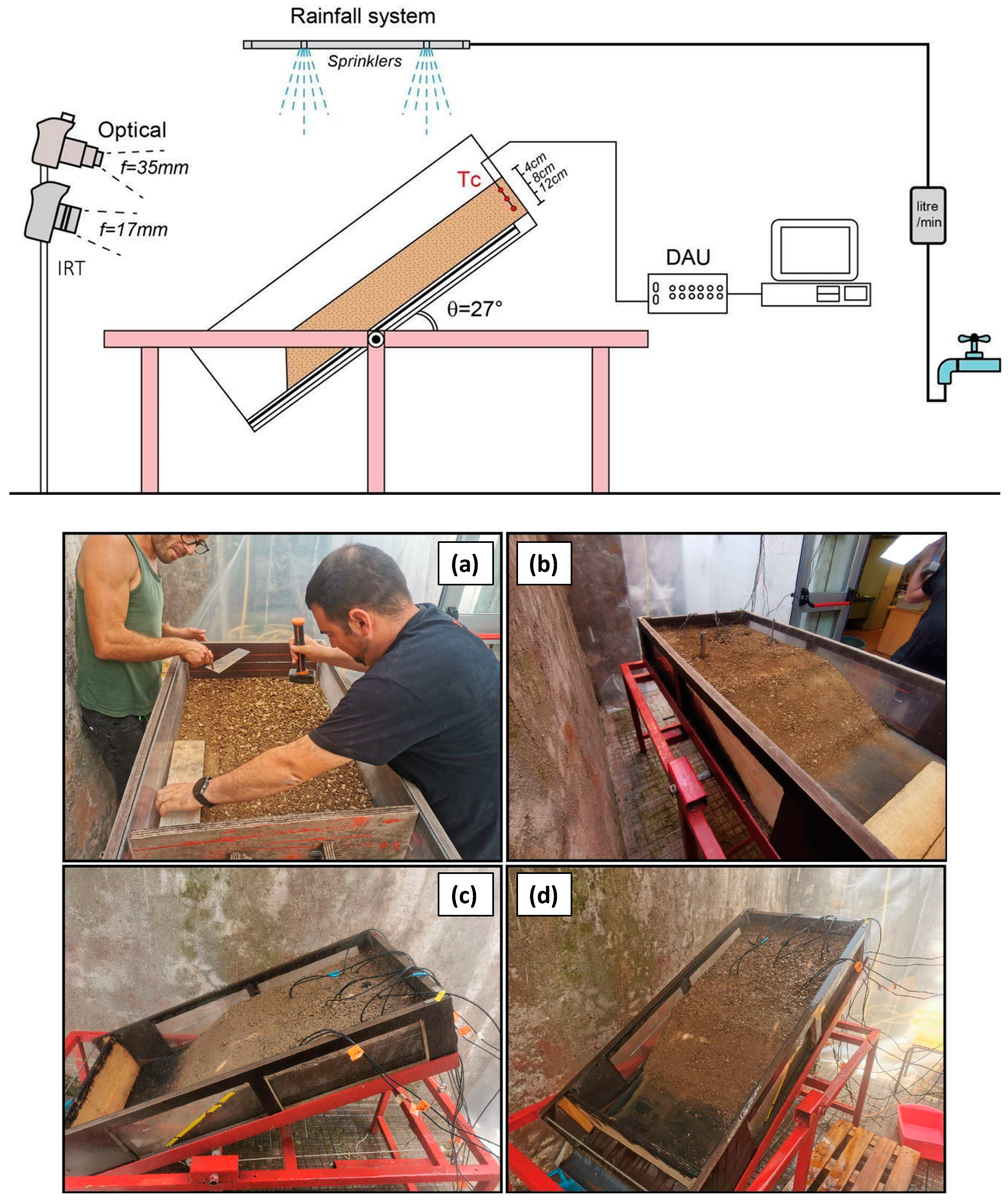
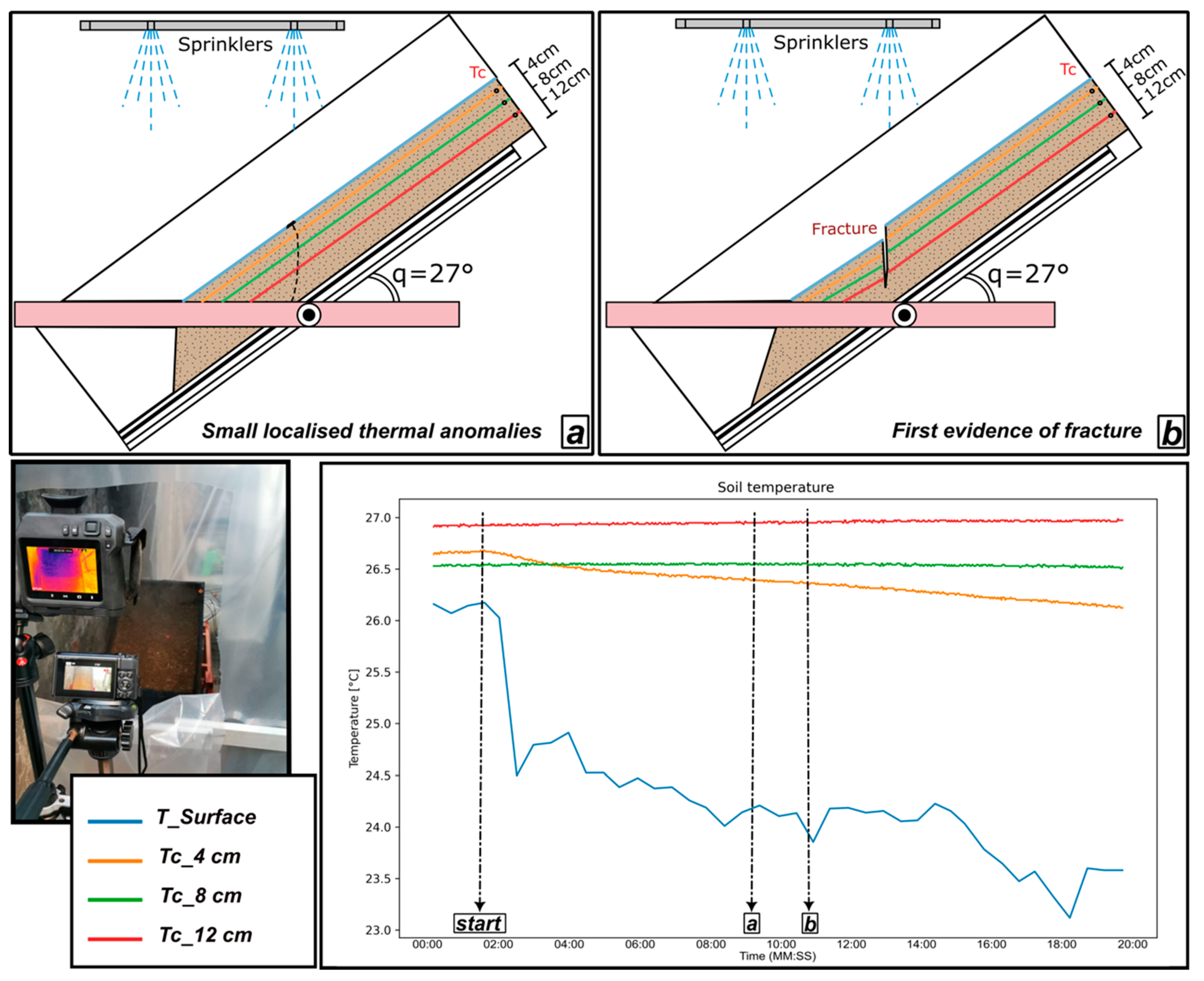
2.1. Description of the Experimental Set-Up

The experimental set-up is composed of a rectangular sloping flume apparatus 100 cm long, 60 cm wide, and 20 cm high, filled with a granular soil mixture collected from the Cinque Terre field laboratory [39]. Both sides of the metallic framework were made of thick plexiglass to allow the visual observation of the wetting and triggering processes along the lateral soil section. A rough plastic panel was applied to ensure basal friction between the soil particles and the base of the flume apparatus and avoid generalized displacement of the filling material. A stiff permeable barrier was fixed in front of the soil to contain it after the failure (Figure 1).
The soil material used for the experiments was composed of silty gravel (GM according to the Unified Soil Classification System (USCS)), i.e., composed of more than 50% of gravel with a range of 11–25% of silty fine (ML according to the Casagrande Plasticity Chart) and reconstituted at the site density according to the in situ natural bulk density, equal to 14.6 ± 1.05 kN/m3. The granular soil mixture was posed on a squared box by overlaying four compacted layers 4 cm thick parallel to the flume base. Given the fixed rectangular geometry, the soil weight required to fill that volume was calculated considering the fixed initial water content. Finally, a slope was created in the termination of the material. Three thermocouples (Tc) were inserted into the soil at depths of 4, 6, and 12 cm below the surface to control the temperature at different depths during the test, connected to a Data Acquisition Unit (DAU) system.
Three different tests were conducted with soil initial water content (w0) of 9% (T1), 14% (T2), and 16% (T3). Soil water content was imposed before placing the soil into the flume by wetting a specific quantity of oven-dried soil with the amount of water needed to reach the desired initial water content value. After, the soil was set into the flume and the water content was checked by sampling the soil at different points.
To artificially reproduce the rainfall process, two sprinklers consisting of individual nozzles were placed at a height of 3 m from the flume, at a distance such that the free surface was evenly wetted, and the raindrop size and impact energy distribution was consistent with the scale of the experiment. To ensure the correct functioning of the system, the supplied water pressure was kept constant at 3.2 bar, resulting in a steady rainfall input of approximately 1 mm/min.

2.2. Description of Sensors

During experiments, a video camera was used to monitor the time occurrence and location of failure initiation, while concurrent thermographic acquisitions were carried out every 30 s to frame surface temperature evolution during the artificial rainfall event. For this work, a Canon PowerShot SX730 HS (Canon Inc., Tokyo, Japan) and a FLIR T840 model (Teledyne FLIR, Wilsonville, OR, USA) IRT imaging camera were used, both installed on a fixed tripod at 2.40 m from the flume. To have the same viewpoint, the two cameras were installed at the front of the experimental channel. The characteristics of the cameras are shown in Table 1 below.
An infrared thermal camera typically consists of an optical system, a detector, and a signal processor. The principle of infrared thermography (IRT) relies on the acquisition of energy reflected by an object in the infrared band of the electromagnetic spectrum, and on the conversion of such energy in temperature according to the Stefan–Boltzmann “black-body” law, given a specific emissivity [40]. The phenomenon is known as “thermal radiation,” which can be detected from a distance and used to measure the radiant temperature of the analysed environment [41]. In the electromagnetic spectrum, infrared (IR) is between visible light and microwaves. The infrared band extends from approximately 430 MHz (with a wavelength of about 0.7 μm) to 300 GHz (with a wavelength of about 103 μm). This band can be divided into several sub-bands: near-infrared (with wavelengths between 0.7 and 1 μm), short-wave infrared (between 1 and 3 μm), mid-wave infrared (between 3 and 5 μm), and long-wave infrared (between 8 and 14 μm). Unlike visible light, infrared wavelengths are longer, making this radiation generally invisible to the human eye. However, it can be detected using specifically designed sensors, such as infrared thermal cameras. In a thermal image, a false-colour scale is used to represent the temperature of each pixel. The temperature of each pixel is based on the infrared radiance detected in the area under consideration. Different temperature values are then mapped to different colours, creating a visual representation of the thermal profile of the object under examination. The emissivity value of soil was evaluated a priori adopting a standard reference method using reference material with a known emissivity.
The use of video footage to acquire high sampling rate optical data and study very rapid processes with a PhotoMonitoring approach has shown encouraging results in some applications for the dynamic study of structures [42]. This application could also be used to study processes such as rainfall triggering landslides. In this work, the same principle shown by [42] was used, i.e., recording a video from a fixed position in order to acquire high-frequency optical data during experimental flume tests.
Video recording during the analogue laboratory tests was performed using a Canon PowerShot SX730 HS camera, mounted on a tripod at 2.40 metres from the flume test as shown in Figure 1. The video camera was programmed to acquire an image at a frequency of 30 Hz, at 30 frames per second (fps) and in Full HD resolution (1920 × 1080). The characteristics of the video camera are shown in Table 1.

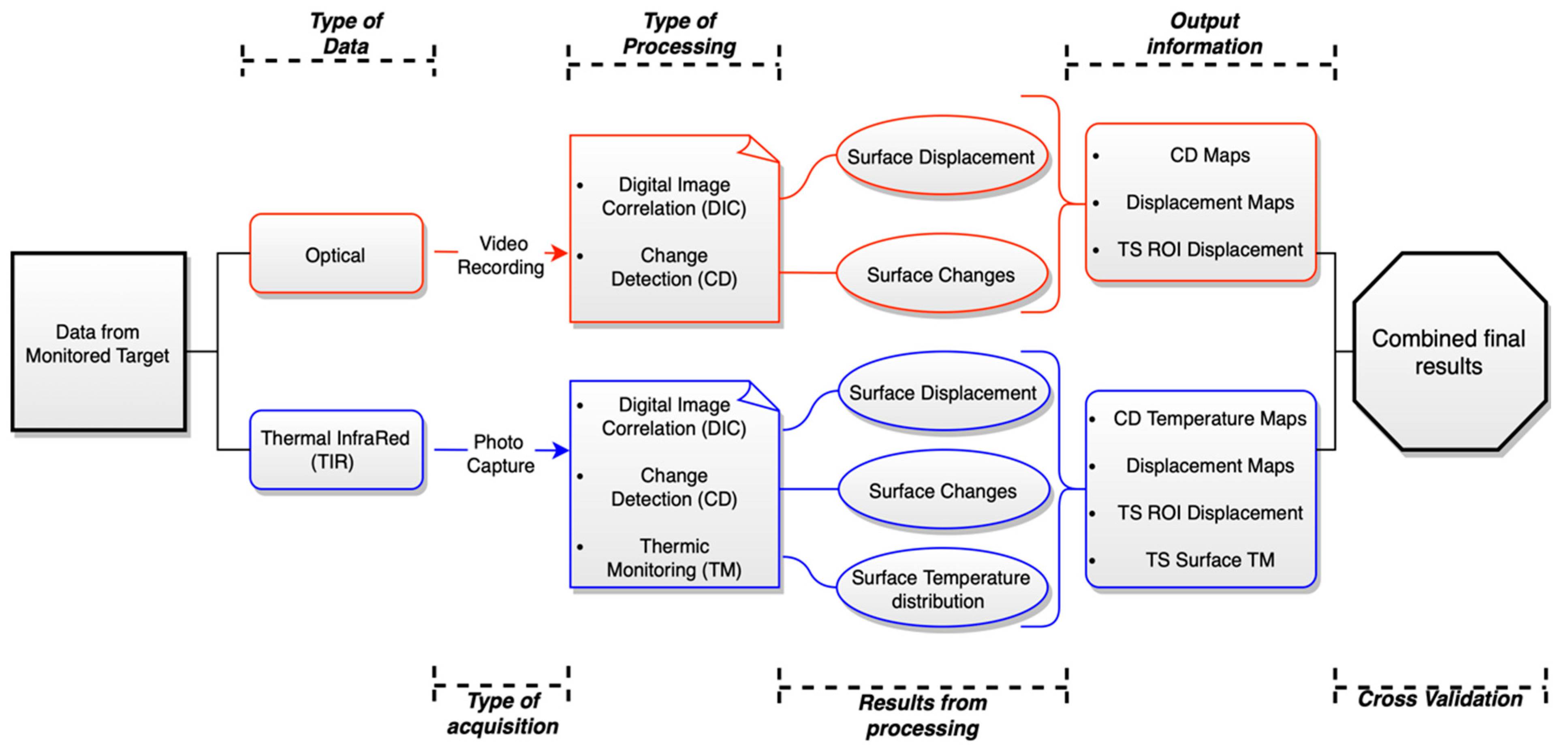
2.3. Remote Sensing Technique (RTS)

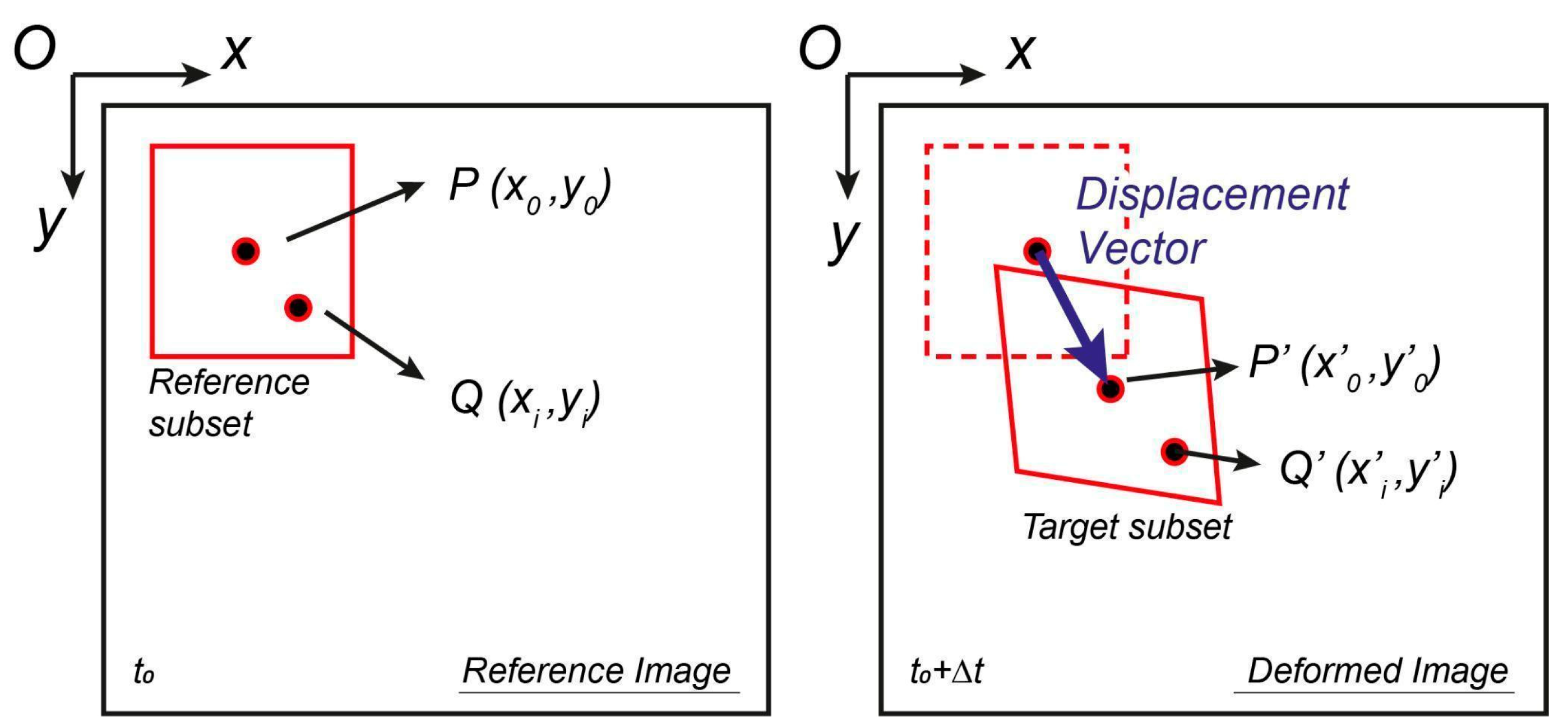
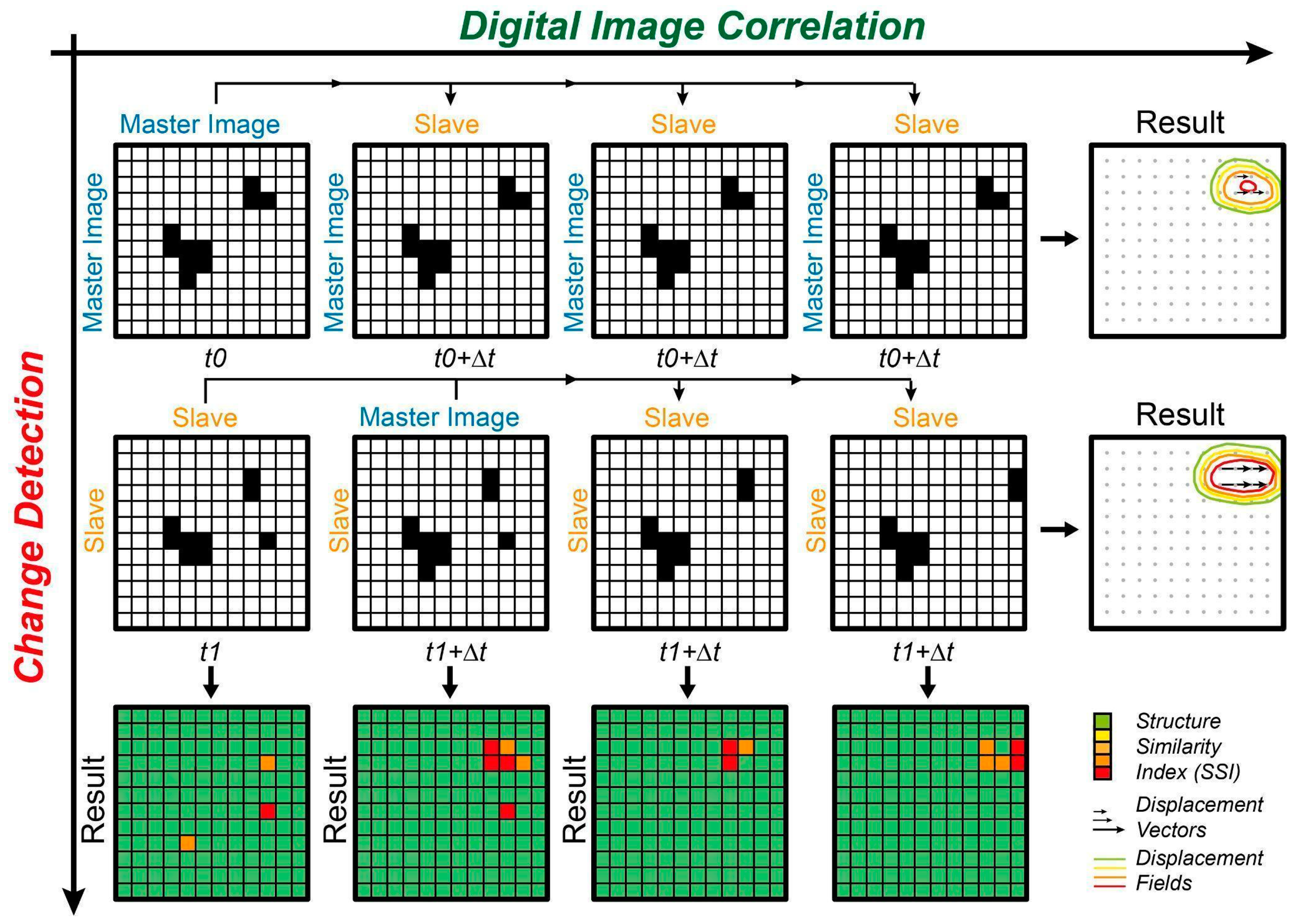
2.3.1. Principles of PhotoMonitoring

PhotoMonitoring is an innovative monitoring solution that utilizes advanced digital image processing algorithms to harness the extensive utilization of optical/multispectral, hyperspectral, and radar sensors on a global scale [12]. By employing digital image processing techniques, PhotoMonitoring enables the extraction of considerable change information (change detection) and/or analysis of displacement of a target object in two (or more) pictures (digital image correlation) (Figure 2).
The versatility and abilities of this method have proven to be particularly advantageous in identifying and monitoring landslides, especially when compared to traditional in situ techniques that can be costly and time-consuming in terms of manpower and installation. Advancements in camera technology, along with optical sensing and image processing algorithms, have made technologies like DIP highly appealing [13].
Digital image correlation (DIC) is an optical-numerical measurement technique that provides full-field 2D surface displacements or deformations in a direction normal to the line of sight. The accuracy of the displacement field maps obtained from DIC algorithms depends on the spatial and temporal resolution of the dataset. DIC involves registering two or more images of the same scene and extracting displacement fields to determine the best match. Deformations are calculated by comparing and processing co-registered digital images of the object’s surface before and after the deformation event [43]. Theoretically, DIC displacement measurements can achieve sub-pixel accuracy of approximately 1/50th of a pixel [44] under optimal conditions. However, challenges related to image orientation, co-registration, topographical distortion, instrumental and atmospheric noise, temporal and spatial decorrelations, and co-registration errors may limit the attainment of these accuracy values [11,45]. In many cases, DIC enables displacement and deformation measurements without the need for installing sensors or reflectors on the object, making it a fully remote measurement system [46]. However, a random speckle pattern on the object’s surface is a fundamental requirement for obtaining a unique solution in the correlation process [11].
The analysis presented here was performed using IRIS software (version 23.1), developed by NHAZCA S.r.l., a start-up of the ‘Sapienza’ University of Rome, which enables change detection (CD) and DIC, using various algorithms from the relevant literature [47,48] and customised specifically for this purpose.
The change detection method employed in the software utilizes the Structural Similarity Index Method (SSIM), a perception-based model. SSIM considers image degradation as a change in the perception of structural information, incorporating factors such as luminance and contrast masking.
The equation found in the SSIM literature is shown below.
  S S I M   x , y = [ l x , y ] α · [ c x , y ] β · [ s x , y ] γ
Here, l is the luminance (used to compare the brightness between two images), c is the contrast (used to differ the ranges between the brightest and darkest region of two images), s is the structure (used to compare the local luminance pattern between two images to find the similarity and dissimilarity of the images), and α, β, and γ are the positive constants [47]. The algorithm will return an index that expresses the images similarity, i.e., in which a value of ‘0’ will indicate a total change between the master and slave image, while a value of ‘1’ will be associated with areas where no change between the two analysed images was identified.
The term “structural information” highlights the strong interdependence and spatial proximity of pixels, providing important visual object information within the image domain. In image quality assessment, SSIM is one of the widely used techniques, but there are other methods such as Mean Squared Error (MSE), Universal Image Quality Index (UIQI), Peak Signal Noise Ratio (PSNR), Human Vision System (HVS), and Feature Similarity Index Method (FSIM); these methods estimate perceived quality by measuring the similarity between the original image and the secondary image [47]. As noted by [49], SSIM shows great potential for use in change monitoring due to the good quality and accuracy of the results.
The CD method implemented in the IRIS software uses the Structural Similarity Index Method (SSIM) algorithm to assess image quality based on a reference image. It operates on a local scale, iteratively assessing image similarity within small subsets of pixels (window size), allowing automatic identification of regions where changes have occurred. In this research, the analysis was conducted using a moving window size of 32 pixels. The IRIS software used for this work returns a raster map with an SSIM value for each pixel. The map is associated with a colour bar that varies from ‘green’, which is associated with the SSIM value ‘1’ (no change identified between the two images), to ‘blue’, which is associated with the SSIM value ‘0’ (total change between the two images).
The displacement analysis method implemented in the IRIS software, on the other hand, involves different types of algorithms that exploit different analysis techniques (feature tracking, phase correlation, and an Optical Flow algorithm). Displacement maps can be created through a single pair of images (single analysis approach) or through a stack of images depicting the same area (multi-master approach) [12]. In this second case, the use of a stack of images instead of a single pair allows an advanced application of the DIC technique (multiple-pairwise image matching correlation (MPIC) or multi-master analysis). This approach involves the use of a sliding master that is compared with a user-selected redundancy with the rest of the images in the stack. This processing makes it possible to obtain for each pixel the time series of the displacement along the N–S and E–W directions and the correlation coefficient (i.e., an estimate of the “quality of the cross-correlation”), with an increase in the signal-to-noise ratio (Figure 3) [9,50,51].
The analysis in this case was conducted using the GEFolkie algorithm, which is a specific implementation of the Optical Flow algorithm [48]. The latter reconstructs the distribution of the apparent velocity of brightness patterns in an image, allowing the derivation of the relative motion of objects with respect to the observer’s plane. Consequently, Optical Flow can provide valuable information about the spatial arrangement of observed objects and the speed at which such arrangements change [52]. In detail, the GEFolkie algorithm is based on moving-window methods, of the Lucas–Kanade type, which employs an iterative, multi-resolution approach, following a pyramid strategy that allows the estimation and identification of large and small displacements [53].
The equation of the GEFolkie algorithm used is shown below:
J ( u ;   x ) = x     S ω   ( x x ) ( f 1   ( I 1   ( x ) )     f 2   ( I 2   ( x + u ( x ) ) ) 2
where ω defines a local window of radius r and size (2r + 1) × (2r + 1), thus ω(x) = 1 iff |x| ≤ r and 0 else; f1 is a function applied to the master image I1, and f2 is a function applied to the slave image I2. These functions, f1 and f2, are designed to project the images in a space where f1 (I1) and f2 (I2) are similar enough to validate the brightness constancy model [53].

2.3.2. Data Processing

Figure 4 illustrates the flow chart showing the steps performed from data acquisition to data processing carried out for the monitoring of rainfall-triggered landslide failures here reproduced in the laboratory and studied with the integrated monitoring system previously described.
The video recording of the experiment began shortly before the start of the rainfall simulation with a sampling rate of 30 fps. IRT images were taken at regular intervals of 30 s from when the test began. The contact sensors (soil temperature) instead recorded at a frequency of one data point every second throughout the test.
The optical data were pre-processed, extrapolating from each video the frames over the first 20 min, encompassing the occurrence of slope failure in the flume, then sub-sampling one frame every 10 s, i.e., 1 frame out of every 300, as described in Table 2.
IRT images were pre-processed directly using the proprietary Research-IR Max FLIR® Software. Colour palettes were standardised and extrapolated in JPEG-Rad format, in order to retain the radiance information. The number of IRT images used was different for each experiment, as can be seen in Table 3, in relation to the time and mode of break-up of the three experiments.
For both datasets, DIC and CD analyses were performed using the IRIS® software. IRT images were also processed directly on the proprietary FLIR® software to extrapolate the surface temperature changes during the test. From these analyses performed on both datasets, displacement and change maps were extrapolated for the entire duration of the experiments.
The final combination and cross-validation steps were conducted by comparing the results obtained from CD and DIC, using both the optical and IRT datasets. Specifically, for the DIC, a time series was extracted from both datasets on a specific region of interest (ROI 1), then a time series was also extracted for a smaller ROI 2 located at the fracture enucleation area. The time series of ROI 1, one from the optical data and another one from the IRT data, were quantitatively compared by calculating the Pearson Correlation Coefficient. This was performed iteratively on all three laboratory tests in order to ensure adequate statistical representativeness.
The Pearson correlation coefficient is a statistical measure that indicates the strength and direction of the linear relationship between two variables. Its value ranges from −1 to 1, with 1 showing complete positive correlation, that is, the two-time series are perfectly correlated in a linear and positive manner, and −1 indicating negative correlation. A value of 0 indicates no linear correlation between the two-time series.
Through this approach, it was possible to assess the similarity between the two measurement techniques and the confidence of the displacement analyses conducted on the IRT images compared to those performed on the optical images. Contact deformation monitoring devices were not available to retrieve ground truth. In addition, the displacement measurements were subjected to advanced validation by direct comparison with measurements performed directly in the laboratory. All displacement maps were returned in millimetres by calculating the Ground Sampling Distance (GSD), i.e., the distance between two consecutive pixel centres measured on the ground. The higher the GSD value of the image, the lower the spatial resolution of the image, and the less detail is visible. In this case, the IRT images had a GSD of 2.3 mm (calculated through FLIR’s Online FOV Calculator) and the optical images had a GSD value of 1.8 mm.

3. Results

The laboratory experiments were performed with three different initial water contents (w0) and showed different behaviour and times to failure. The characteristics of the three experiments are shown in Table 4.
In general, all the tests exhibited a similar behaviour. In each case, an initial stable phase was followed by an incipient slope movement, which was subsequently accompanied by the appearance of fractures on the surface of the earthen slope shortly before generalized failure.
This paper only presents and discusses the results of experiment 2 from 19 July 2022, which was used as a reference for the occurrence of failures. The discussion section includes an evaluation of all three experiments.

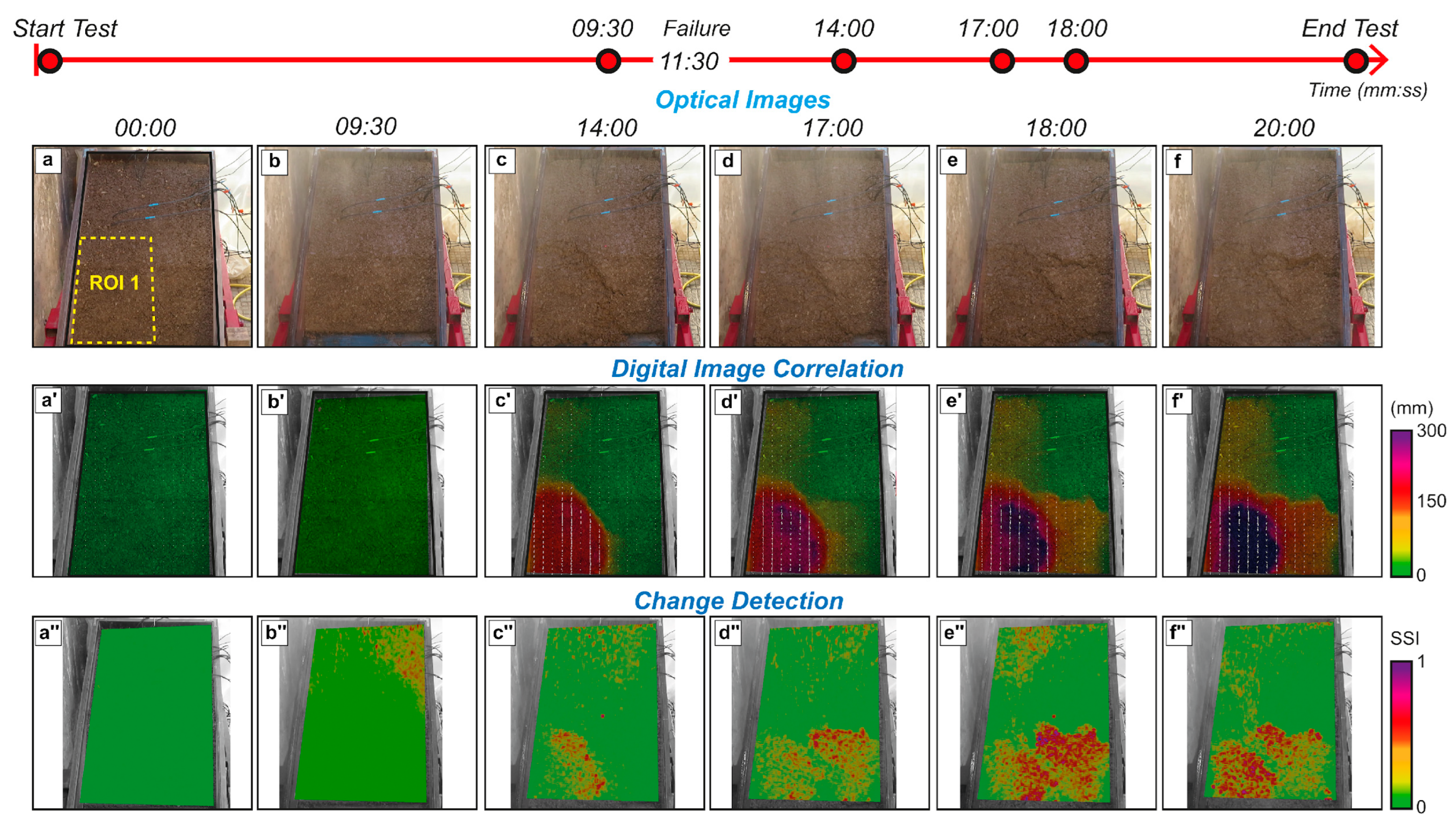
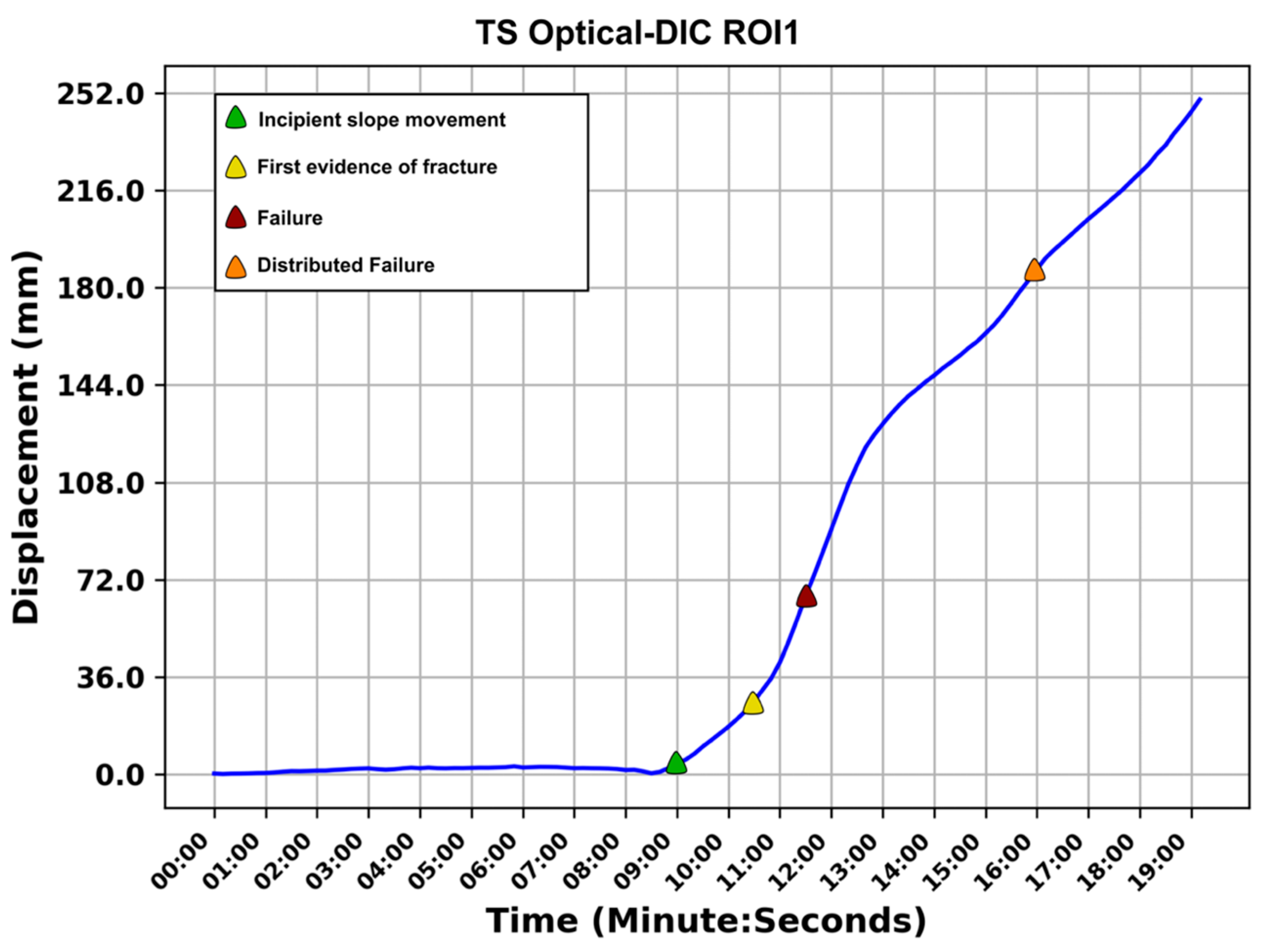
3.1. Results from Optical Camera

As previously described, 3600 frames were extracted from the video. To make the analysis process quicker, a sub-sampling was employed capturing one frame every 10 s (equivalent to one frame out of every 300). The result was a set of 120 frames to be analysed that made it possible to reconstruct the time evolution of the laboratory test (Figure 5). It was observed that the first surface fractures occurred approximately 10:30 min after the start of the experiment. Based on the observed evidence, a specific ROI 1 was selected to extract a displacement time series (TS), highlighted in Figure 5. These selected images from ROI 1 were imported into the IRIS software and analysed following the previously described methods.
Optical-CD analyses performed on the optical images’ frames allowed us to observe how the surface of the slope changed during the experiments by comparing the previous frame with the subsequent frame (sequential frame-by-frame analysis every 10 s). This enabled us to study when and where changes in the slope surface occurred due to the initiation of landslide phenomena. The results revealed that the surface showed consistent evidence of activity, then the formation of first surface fractures from minute 10:30 onwards, and after the beginning of the slope failure. As depicted in Figure 5, the slope surface reproduced in the laboratory experiment displayed evidence of changes in the lower left portion of the image, the active and moving portion. The failure occurred at minute 11:30, and the CD analysis (at minute 16:00) showed the distributed failure phase, with the formation of the fracture in the upper portion of the slope previously unaffected by the failure, as well as the development of a longitudinal fracture from left to right in the test flume. Such a linear fracture represents a translational deformation (and failure) mechanism, well-reproducing infinite slope conditions. Despite the general translational mechanism, a single and coherent rotational surface occurred in the slope toe.
Optical-DIC analysis gave us a quantitative representation of the process evolution, as depicted in Figure 5. In the lower left part was observed a displacement of about 35 mm and a formation of first surface fractures after 10:30 min from the start of the experiment. In the same area, the failure was observed after 11:30 min from the beginning and with a cumulated displacement of about 70 mm. The optical-DIC results, presented in Figure 5, demonstrate a gradual backward movement of the landslide process after 14 min, accompanied by a displacement of approximately another 145 mm in the lower portion. This backward movement was also evident in the optical-CD analyses, which revealed the formation of perimeter fractures in the upper part of the ground slope. Gradual movement in the upper section of the test flume was observable, reaching 40 mm after 18 min from the start of the experiment. In addition to the retrogressive style, it is worth noting that the fracture also affected the right side, exhibiting a significant displacement of approximately 150 mm towards the end of the experiment. After 20 min from the start of the experiment, optical-DIC analysis observed a maximum displacement of approximately 320 mm in the lower section of the test flume (Maximum displacement highlighted in purple in Figure 5). As observed from Figure 5, there is a significant spatial overlap between the results of optical-CD and optical-DIC. In fact, both analyses highlighted the bottom-left area as the region undergoing incipient deformation and then fractures.
Thanks to the optical-DIC analysis performed on the dataset comprising 120 images, it was possible to obtain a temporal displacement series for each pixel within the analysed area (Figure 5a). Within the ROI 1, a temporally averaged series was extracted, enabling the reconstruction of the temporal evolution of the process for that specific area and facilitating the observation of the displacement value in millimetres throughout the entire duration of the test. As depicted in Figure 6, the time series exhibits an initial phase of apparent stability lasting until 9:00 min. From that point onwards, a rapid velocity change is observed, indicating a phase of incipient slope movement followed by the formation of first surface fractures (10:30 min) and the failure of the experimentally simulated slope (11:30 min). From the beginning of the incipient slope movement until the distributed failure (from 9:00 min to the end of the test), two distinct behaviours occur: an initial phase with a velocity of 0.82 mm/s, followed by a phase with a velocity of 0.35 mm/s. This observation indicates that the process tends to decelerate slightly, possibly due to a decrease in the slope angle (probably because the earth mass also becomes partly supported by the sides of the box).

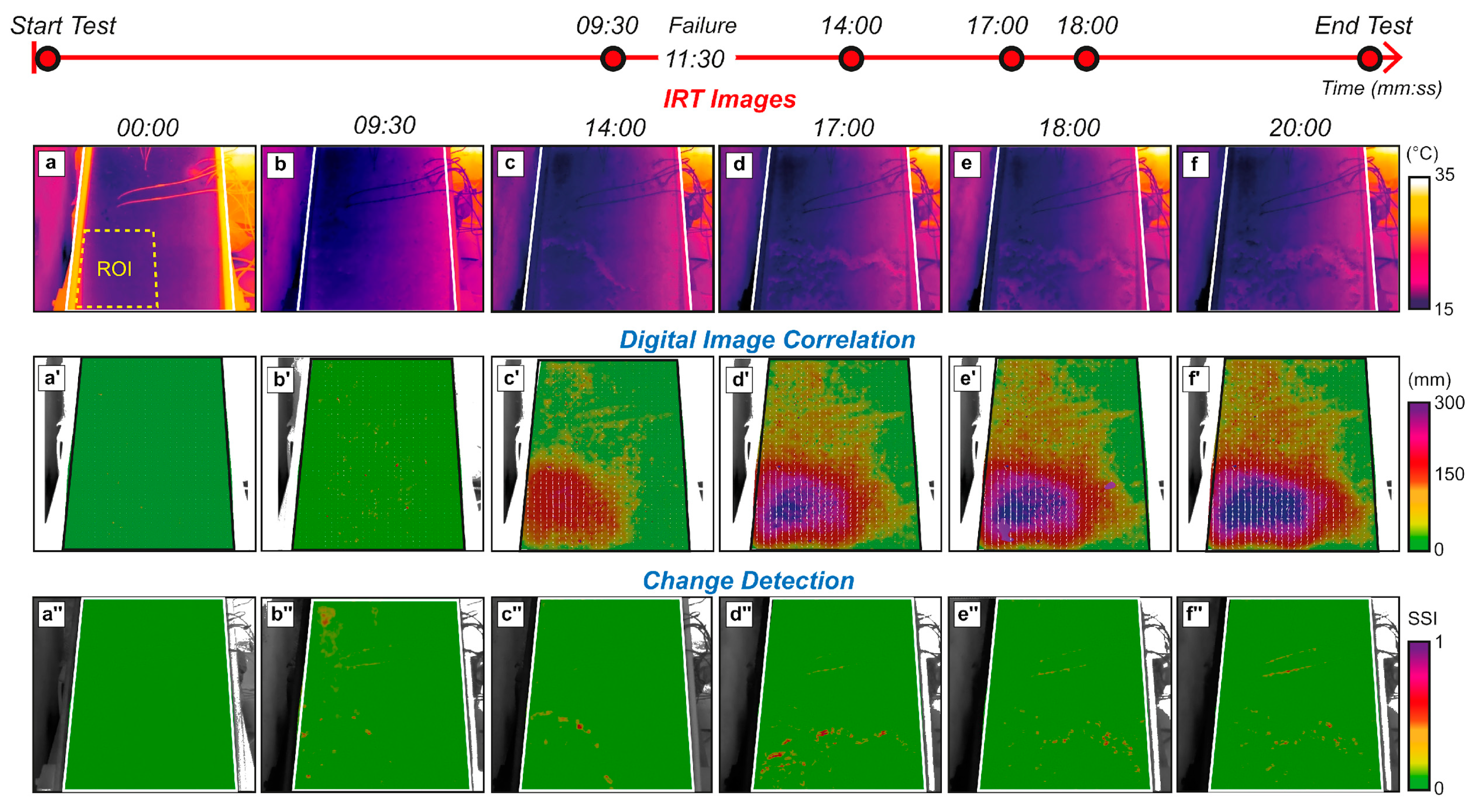
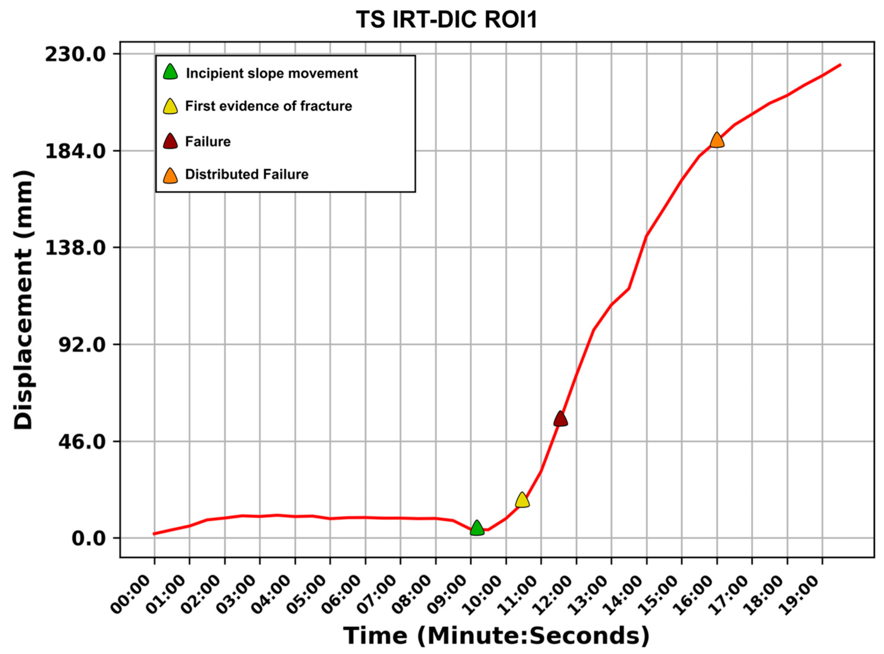
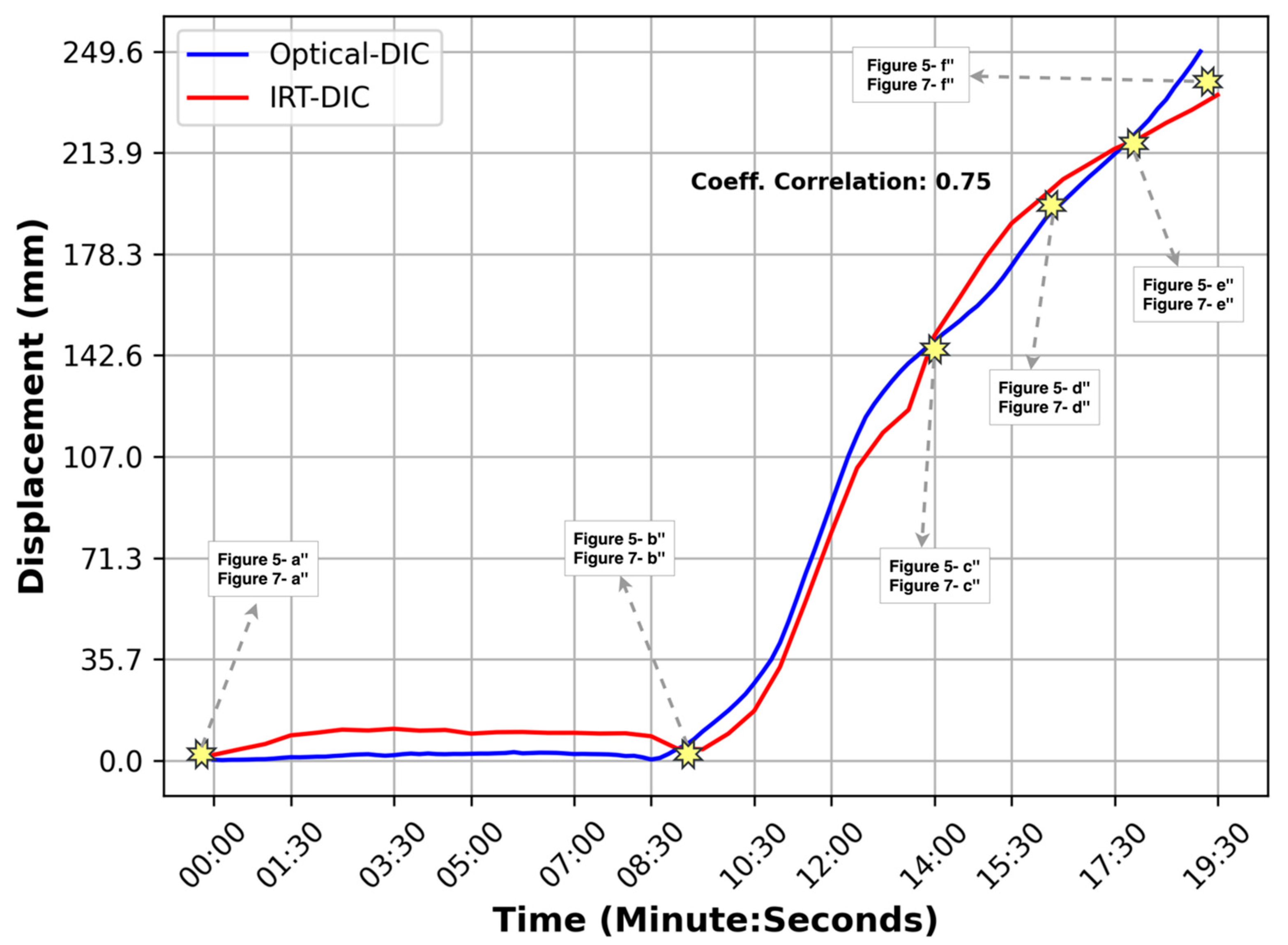
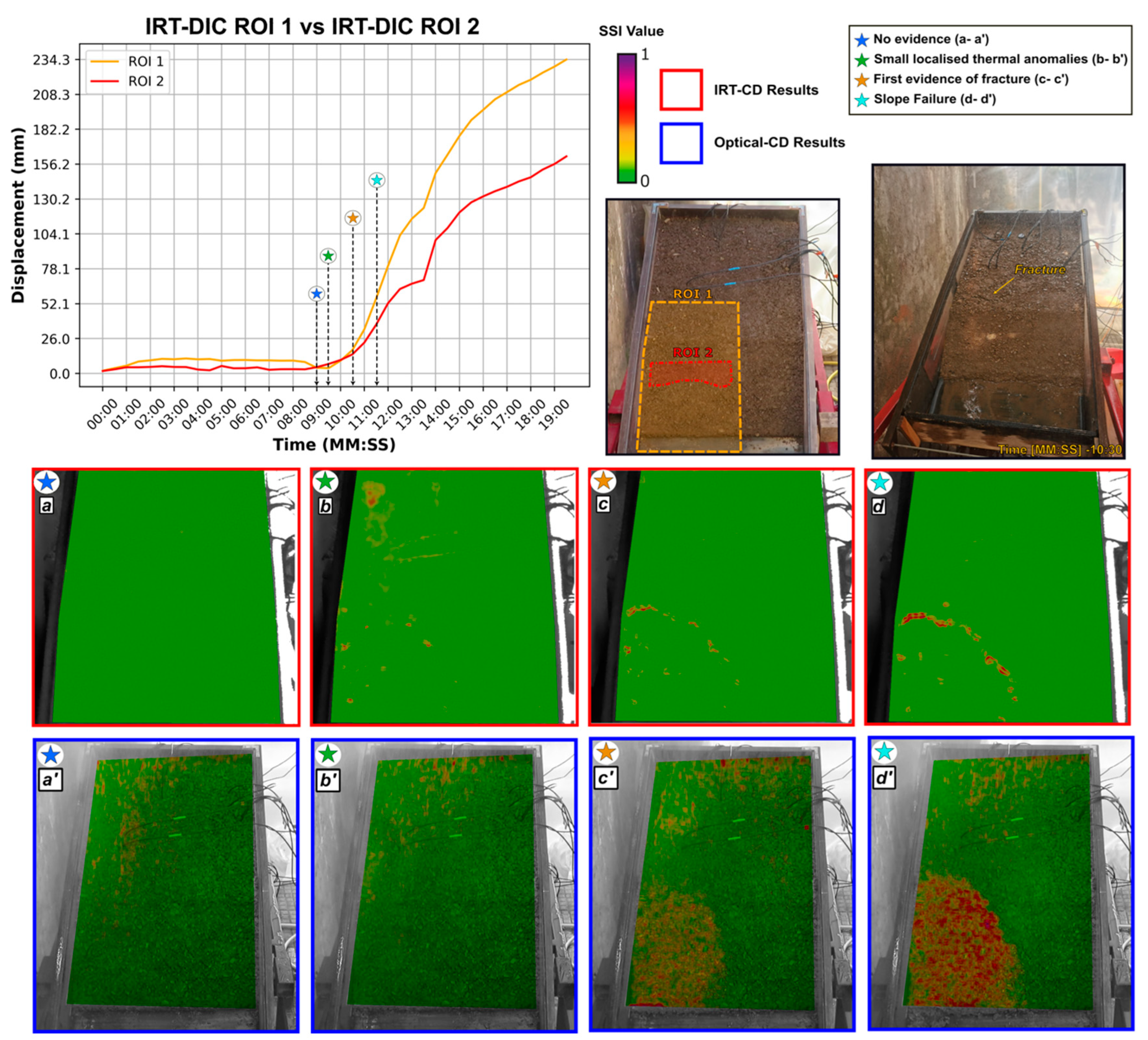
3.2. Results from IRT Sensor

Using IRT images acquired at regular intervals of 30 s, the same DIC and CD analyses performed on the optical images were conducted as described in the Materials and Methods section. The temporal evolution of the laboratory test was thus observed through a sequence of 40 IRT images, as highlighted in Figure 7. The results of the IRT-CD analyses allowed for the observation of changes in the slope related to variations in surface temperature caused by the pluviation, surficial wetting, and initiation of the landslide phenomenon. Analyses were performed, as mentioned above, by comparing the previous IRT image with the next one (sequential image-by-image analysis every 30 s).
The results of the IRT-CD analysis, as shown in Figure 7, identified changes occurring in specific portions of the slope surface, consistent with the area where slope failure occurred. The changes detected by the IRT-CD analysis, represented by the red areas with an SSIM value below 0.5, can be associated with zones that exhibit alterations on the surface of the slope, linked to the presence of positive thermal anomalies caused by the opening of longitudinal fractures (a phenomenon also observed in the corresponding optical images). As reported in Figure 7, after 10:30 from the beginning of the test, during the formation of first surface fractures, positive thermal anomalies (higher temperature than the surrounding area) start to appear in the lower left portion of the flume test. The failure occurred at 11:30 min after the beginning of experiment, and by 14:00 min, the scattered anomalies observed tend to coalesce, clearly indicating the fracture delimiting the portion of the slope where maximum displacement occurs, and a section of the slope detaches. As the laboratory test progressed, after 17 min from the start, the IRT-CD analyses reveal the presence of longitudinal anomalies from left to right, associated with fractures affecting the entire lower part of the slope.
The IRT-DIC analysis was conducted to obtain a quantitative representation of the process evolution using IRT images. The analysis clearly reveals the formation of a fracture zone with a progressive displacement in the lower left portion of the flume (Figure 7). As indicated by the IRT-DIC results, after 14 min from the beginning of the test, the formation of an active area in the lower left part becomes evident, with a measured displacement of approximately 140 mm. Starting from minute 17, a progressive widening of the deformation front is observed, exhibiting a retrogressive trend. In fact, it can be observed that the upper left part of the slope suffers a displacement of approximately 35 mm.
Eventually, after 18 min from the start of the test, the fracture also involved the right side of the slope, displaying a significant widening of the deformation zone. After 20 min from the start of the experiment, through IRT-DIC analysis, a maximum displacement of approximately 320 mm was observed in the lower part of the flume test (maximum displacement highlighted in purple in Figure 7).
The IRT-DIC analyses performed on the dataset of 40 IRT images allowed for obtaining a displacement time series for each pixel within the analysis area. For ROI 1, a temporally averaged displacement series was extracted to reconstruct the temporal evolution of the process for that specific area, thereby observing the displacement values in mm throughout the entire duration of the test. Figure 8 displays the temporal series of the ROI 1 obtained from the IRT images. It is clearly visible that the time series exhibits, although not perfectly centred around zero, an apparent stability phase of the area for up to 9 min from the start of the test. From that point onwards, a rapid change in the gradient is observed, indicating a phase of incipient slope movement followed by the formation of first surface fractures (10:30 min) and the failure of the material under progressive saturation (11:30 min). From the beginning of the slope movement until the distributed failure (from 9.00 min to the end of the test), two different trends are displayed: a first part with a velocity of 0.50 mm/s and a subsequent part with a velocity of 0.28 mm/s. This indicates that the process tends to slightly slow down due to the probable decrease in the slope angle, and the achievement of a new dynamic equilibrium (the earth mass probably also becomes partly supported by the sides of the box), as similarly observed by optical-DIC (Figure 6).

4. Discussion

The performed DIC analyses allowed us to study the shallow landslide replicated in the laboratory and quantitatively reconstruct the evolutionary process leading to failure, with a precision that can reach a resolution lower than the 1/50 of the pixel size [54] and relevant accuracy [55].
Furthermore, the laboratory experiment facilitated the acquisition of measurable and comparable data, ensuring the repeatability and adaptability of the proposed workflow. Indeed, as demonstrated by [35,40], the utilization of the laboratory analogue model has emerged as an extremely effective means to comprehensively explore and understand the behaviour of slopes involved in landslide dynamics. This approach has proven essential for evaluating new monitoring methods, allowing for controlling variables influencing such phenomena, including precipitation, temperature, and soil mechanics.
The obtained results from DIC and CD analyses conducted on the optical and IRT images acquired during the execution of flume test experiments were compared. As reported in Figure 5 and Figure 7, the results qualitatively show the same deformation trend and magnitude of cumulative displacement, which reflected a similar failure mechanism: a fracture nucleating in the bottom-left portion of the flume after 10:30 min from the beginning of the test, which then evolved with a retrogressive and roto-translational failure.
For a quantitative comparison, as shown in Figure 6 and Figure 8, the two time series were extracted from the DIC displacement analyses for the same ROI 1, one obtained from optical data and the other from IRT data. Subsequently, these two time series were quantitatively compared using a Pearson correlation coefficient.
As reported in Figure 9, the IRT- and optical-DIC time series exhibit a high correlation with a coefficient of 0.75, indicating a good correspondence among the series and the suitability of the two techniques. Approximately 9 min after the start of the test, a significant incipient slope movement phase can be observed, followed by the appearance of the first fracture and the subsequent failure of the slope. Both time series are characterised, from 9:00 min onwards, by two different slope angles, the first one constant up to 14:00 min (speed of approx. 0.82 mm/s), which subsequently changes, indicating a tendency to decelerate due to the reduction of the slope (speed of approx. 0.35 mm/s).
To study the quantitative difference between the two time-series, the Mean Absolute Percentage Error (MAPE) was calculated, which expresses the average percentage error. This value was calculated without considering the initial part (0–9:00 min). In this stage, the IRT-DIC analysis has an overestimated error of displacement. In fact, the displacement in this stability phase is not perfectly zero. Consequently, throughout this initial part, the IRT time series (in red) consistently appears above the optical time series (blue line in Figure 9). This is due to the surface temperature change that occurred following the opening of the rain irrigators in the initial phase of the test, which are sensitive to IRT images but not to optical ones. From the analysis of the second part of the time series, it is evident that the DIC analyses conducted with IRT images tend to underestimate the displacement by approximately 3.6% compared to the DIC analyses performed with optical images (considered as a benchmark and validated by the displacement measured in the laboratory). In this case, it is possible to see how the optical-DIC is slightly more precise and accurate than the IRT-DIC; in fact, it is able to better discern the beginning of the phase of incipient slope movement. It must be considered, however, that the techniques of optical-DIC are more used in the literature, and therefore more evolved from a computational point of view [56].
The correlation analyses conducted on DIC results reported for experiment 2 were also carried out for the other laboratory experiments. Specifically, the time series obtained from DIC analyses conducted with optical data were compared with those obtained from DIC analyses conducted with thermal data for the same region of interest (ROI). The correlation index values for all three experiments are presented in Table 5 below.
The correlation coefficient values highlight a good correspondence between the time series obtained with optical images and those obtained with thermal images over the three experiments (the average is about 0.72). This result confirms that, through the IRT-DIC analyses, it is possible to quantitatively reconstruct the deformation process induced in the flume, introducing a small underestimate but enabling the monitoring of the soil surface temperature evolution during and after rainfalls and following the deformation process up to failure. In addition, IRT-DIC analyses could allow 24-h monitoring in contrast to those of optical-DIC, which are not applicable, for example, during the night, making the technique suitable for continuous monitoring and can also be used in an early warning system after more in-depth studies.
Conversely, the CD analyses were used to compare step-by-step changes occurring on the surface of the earth slope, investigating any signs of incipient failure. As the results show (Figure 5 and Figure 7), the surface of the slope did not undergo any noticeable changes until after the first fracture had appeared (10:30 min). The results obtained from the optical-CD clearly show an area with low SSIM values (red area in Figure 5), representative of the large portion where significant surface changes occur due to the deformation affecting the lower left portion (Figure 5b″–f″).
In contrast to optical-CD, the results obtained from IRT-CD allow the observation of numerous small changes (with low SSIM values) that result from the appearance of positive thermal anomalies on the surface. These thermal anomalies, clearly visible, are attributable to the enucleation of the fractures. For this difference, IRT-CD analysis was better suited and more effective than optical-CD for a more detailed examination of the fracture geometry and their growth over time (Figure 7b″–f″).
The presence of these specific positive thermal anomalies on the surface is primarily due to the thermal difference produced between the surface, cooled by the presence of infiltrating water, and the deeper soil, which is affected with a temporal delay by the cooling effect of water. These thermal contrasts begin to be seen from the formation of the first surface fractures (10:30 min), when the fracturing slowly exposes the deepest soil. This is further confirmed by comparing the surface temperature to the temperature measured using the thermocouples located at depths of 4, 6, and 12 cm below the surface (Figure 10). From the analysis of Figure 10, an important drop of approximately 2 °C in surface temperature is clearly observed around 2 min after the start of the test.
Through the results of IRT-CD, it was possible to accurately reconstruct the fracture geometry due to the emergence of thermal anomalies. To achieve this, a detailed study of the occurrence of these positive thermal anomalies was conducted, correlating the IRT-CD results with the time series obtained through IRT-DIC. This allowed for an understanding of the deformation state of the test in the moment when surface thermal anomalies related to the fracture phase appeared. As shown in Figure 9, the appearance of surface thermal anomalies occurs after the incipient slope movement phase, approximately 10:30 min after the start of the test.
However, thanks to the detailed analysis and the correlation between IRT-CD and IRT-DIC results, small and localized positive thermal anomalies were observed at 9:30 min from the start of the test, as depicted in Figure 7b″. These small anomalies, identified exclusively through IRT-CD results and not visible to the naked eye or through optical-CD, appear in the lower left portion of the slope before the appearance of surface fractures. In fact, as the test progressed, these anomalies evolved to form the first fracture and the subsequent collapse of the slope into the soil (Figure 7b,b′,b″ and Figure 10).
To understand the origin of the thermal anomalies observed before the fracture, which were not caused by the thermal difference produced between the surface and the deeper soil, a more detailed time series was extracted. This time series was obtained from the IRT-DIC analysis within ROI 2, located within ROI 1, in the portion where these thermal anomalies were registered. The primary aim was to determine if these thermal anomalies were caused by a small displacement that opened the fracture, or if they were caused by drainage-induced settling effect before the first fracture appeared. To better understand the origin of these pre-failure thermal anomalies, the results of IRT-CD and IRT-DIC were compared (Figure 11).
As reported in Figure 11, the surface thermal anomalies occur 2 min before the slope failure, which is preceded by the formation of a surface fracture. It is evident that the area in which the thermal anomalies are observed at 9:30 min corresponds to the sector in which a continuous fracture has developed (Figure 11c), as these thermal anomalies progressively coalesce into a main fracture that allows roto-translational sliding at the foot of the slope.
Considering what has been observed, it is therefore assumed that the appearance of these thermal anomalies is linked to a slight pre-fracture settlement and internal slope drainage, which is not visible to the naked eye and in the visible bands.
This occurs in response to the infiltration effect of water from the rainfall system and the consequent development of a saturated waterfront migrating downward (e.g., [35,39]). In fact, recent reports [57,58,59] have concluded that, for rainfall-induced translational slides in terrains of homogeneous soil, the sliding failure can be categorized as occurring in two major phases: the infiltration phase and the saturation phase. In the infiltration phase, rainwater infiltrates cause the advance of the wetting zone. If the failure takes place in this phase, the failure plane can occur at specific depth depending on slope angle, rainfall intensity, soil mechanical parameters, and matrix suction conditions. The saturation phase occurs during the rising of the water table, which initially occurs after rainwater reaches the impermeable interface [60]. If failure occurs in the infiltration phase, precursor signs may occur relatively close to the final stages of landslide triggering, and therefore conventional instruments are not suitable to identify it [61]. On the other hand, if failure occurs during the saturation phase the failure plane occurs only at the impermeable interface and with instruments like soil deformation sensors at high frequency, installed in the subsurface, it is possible to investigate the precursors signals [62].
The approach tested in this work, i.e., the combined use of IRT-CD and IRT-DIC, turns out to be able to reconstruct the landslide process by extrapolating time series, and also to identify thermal anomalies (Figure 11b) directly relatable to the specific failure mechanism that can be registered in advance (before the fracture nucleation and slope failure).
However, further studies and tests are needed to extend this application to real-world scenarios where geometric and triggering conditions are not controlled and cause–effect relationships unclear. The major potential of this methodology resides in the versatility of the sensors used for the analysis, which allows for a wide range of flexibility in real-world applications. This includes the possibility of using IRT sensors with different focal length and spatial and temporal resolutions and/or in combination with optical cameras with higher geometric resolution, offering higher measurement sensitivity. The reported findings, if scaled up for real-life monitoring applications, could create a low-cost photomonitoring technique capable of operating in both day and night conditions that could also be integrated into a more complete monitoring system able to provide near real-time information in a broader spectral band.

5. Conclusions

In this study, we present an integrated approach to monitor shallow landslides triggered by rainfall, employing DIP techniques utilizing optical and IRT data. Two different methods of image analysis have been adopted: DIC and CD. While these techniques are more frequently used with optical data, the use of IRT data for monitoring shallow landslides is a relatively new and promising research application. The adopted approach, applied at the scale of a laboratory experiment, enabled us to accurately reconstruct the entire landslide process throughout its stages of stability, incipient slope movement, and slope failure.
DIC and CD analysis were adopted, integrating potential of infrared thermography and optical data by deriving data on displacement, velocity, surface morphological changes and temperature variations.
IRT-DIC analyses showed a high reliability and accuracy in defining the pattern and magnitude of slope displacement, highlighting the same deformation phases observed in the optical-DIC analyses. Cross-correlation among IRT-DIC and optical-DIC derived time series resulted in a good correlation coefficient for all the tests conducted. Notably, both IRT-DIC and optical-DIC analyses results showed the presence of an incipient slope movement phase about two minutes before the slope failure and without any type of surface evidence. In addition, the combination of the IRT-CD and IRT-DIC results showed the presence of anomalies in the SSI value, given by slight thermal anomalies about one minute before the slope failure and without the presence of surface evidence of fracture.
Our results, in particular the identification of the incipient slope movement phase and the small thermal anomalies, can be considered potential precursor signs of slope failure, providing convincing evidence of the reliability of DIP with the combination of optical and thermal data.
More generally, this methodology has proven its reliability on a laboratory scale, promising for potential real-scale applications. The obtained results testified the value of IRT and Optical combination in landslides monitoring, especially if scaled for early warning purposes and transferred to real scenarios, where the delay between precursor signal and failure can be large. Unlike optical images, the application of DIP on thermal data improves the ability to collect data even during the night-time, boosting image analysis potential for early warning systems.
The optical and IRT-DIP techniques introduced in this study represent a tool for monitoring the deformation processes associated with shallow landslides. Although the full scalability of this approach to natural processes requires further investigation, the obtained results represent a promising example of integrated monitoring functional for defining appropriate and cost-effective strategies for shallow landslide risk mitigation and safety improvement in vulnerable areas.

Author Contributions

Conceptualization, G.M.M., M.F., A.C. and P.M.; methodology, A.C. and G.M.M.; software, A.C.; validation, A.C., G.M.M. and M.F.; formal analysis, A.C.; investigation, A.C., G.M.M. and M.F.; data curation, G.M.M. and M.F.; writing—original draft preparation, A.C.; writing—review and editing, A.C., G.M.M., M.F., P.M. and G.S.M.; visualization, C.E.; supervision, P.M., G.S.M. and C.E.; project administration, C.E.; funding acquisition, G.M.M., P.M. and C.E. All authors have read and agreed to the published version of the manuscript.

Funding

This study has been supported by the Sapienza University of Rome project, “Analysis of 2D and 3D thermal response of rocks and soils in landslide triggering conditions through site and laboratory experiments” (Sapienza University of Rome—Year 2019, P.I. Gian Marco Marmoni) and by the European Union—NextGenerationEU—Mission 4 “Education and Research”—Component 2 “From Research to Business”—Investment 3.1 “Fund for the realization of an integrated system of research and innovation infrastructures”—Project IR0000037—GeoSciences IR—WP3 Landslides and Sinkholes. Operative Unit 26. Flume tests and field sampling were also funded in the frame of the project “Grandi frane in roccia e frane superficiali a cinematica rapida in aree montane: metodi per la previsione temporale e spaziale (prediction and susceptibility)” by DARA—Dipartimento per gli Affari Regionali e le Autonomie within the agreement between DARA and the Earth Sciences Department of Sapienza University of Rome.

Data Availability Statement

The data presented in this study are available on request from the corresponding author.

Acknowledgments

The authors wish to acknowledge Javad Rouhi and Davi Silvestri Benjamin for their valuable support in flume tests, and Marco Fiorio for his support in thermal image analysis and software customisation.

Conflicts of Interest

The authors declare no conflict of interest.

References

  1. Haque, U.; Blum, P.; Da Silva, P.F.; Andersen, P.; Pilz, J.; Chalov, S.R.; Malet, J.-P.; Auflič, M.J.; Andres, N.; Poyiadji, E.; et al. Fatal Landslides in Europe. Landslides 2016, 13, 1545–1554. [Google Scholar] [CrossRef]
  2. Klose, M.; Maurischat, P.; Damm, B. Landslide Impacts in Germany: A Historical and Socioeconomic Perspective. Landslides 2016, 13, 183–199. [Google Scholar] [CrossRef]
  3. Casagli, N.; Intrieri, E.; Tofani, V.; Gigli, G.; Raspini, F. Landslide Detection, Monitoring and Prediction with Remote-Sensing Techniques. Nat. Rev. Earth Environ. 2023, 4, 51–64. [Google Scholar] [CrossRef]
  4. Canuti, P.; Casagli, N.; Ermini, L.; Fanti, R.; Farina, P. Landslide Activity as a Geoindicator in Italy: Significance and New Perspectives from Remote Sensing. Environ. Geol. 2004, 45, 907–919. [Google Scholar] [CrossRef]
  5. Gunzburger, Y.; Merrien-Soukatchoff, V.; Guglielmi, Y. Influence of Daily Surface Temperature Fluctuations on Rock Slope Stability: Case Study of the Rochers de Valabres Slope (France). Int. J. Rock Mech. Min. Sci. 2005, 42, 331–349. [Google Scholar] [CrossRef]
  6. Dai, F.C.; Lee, C.F.; Ngai, Y.Y. Landslide Risk Assessment and Management: An Overview. Eng. Geol. 2002, 64, 65–87. [Google Scholar] [CrossRef]
  7. Mantovani, F.; Soeters, R.; Van Westen, C.J. Remote Sensing Techniques for Landslide Studies and Hazard Zonation in Europe. Geomorphology 1996, 15, 213–225. [Google Scholar] [CrossRef]
  8. Chae, B.-G.; Park, H.-J.; Catani, F.; Simoni, A.; Berti, M. Landslide Prediction, Monitoring and Early Warning: A Concise Review of State-of-the-Art. Geosci. J. 2017, 21, 1033–1070. [Google Scholar] [CrossRef]
  9. Mazzanti, P.; Caporossi, P.; Muzi, R. Sliding Time Master Digital Image Correlation Analyses of CubeSat Images for Landslide Monitoring: The Rattlesnake Hills Landslide (USA). Remote Sens. 2020, 12, 592. [Google Scholar] [CrossRef]
  10. Guerriero, L.; Di Martire, D.; Calcaterra, D.; Francioni, M. Digital Image Correlation of Google Earth Images for Earth’s Surface Displacement Estimation. Remote Sens. 2020, 12, 3518. [Google Scholar] [CrossRef]
  11. Caporossi, P.; Mazzanti, P.; Bozzano, F. Digital Image Correlation (DIC) Analysis of the 3 December 2013 Montescaglioso Landslide (Basilicata, Southern Italy): Results from a Multi-Dataset Investigation. IJGI 2018, 7, 372. [Google Scholar] [CrossRef]
  12. Mazza, D.; Cosentino, A.; Romeo, S.; Mazzanti, P.; Guadagno, F.M.; Revellino, P. Remote Sensing Monitoring of the Pietrafitta Earth Flows in Southern Italy: An Integrated Approach Based on Multi-Sensor Data. Remote Sens. 2023, 15, 1138. [Google Scholar] [CrossRef]
  13. Oats, R.C.; Dai, Q.; Head, M. Digital Image Correlation Advances in Structural Evaluation Applications: A Review. Pract. Period. Struct. Des. Constr. 2022, 27, 03122007. [Google Scholar] [CrossRef]
  14. Mugnai, F.; Caporossi, P.; Mazzanti, P. Exploiting Image Assisted Total Station in Digital Image Correlation (DIC) Displacement Measurements: Insights from Laboratory Experiments. Eur. J. Remote Sens. 2022, 55, 115–128. [Google Scholar] [CrossRef]
  15. Spampinato, L.; Calvari, S.; Oppenheimer, C.; Boschi, E. Volcano Surveillance Using Infrared Cameras. Earth-Sci. Rev. 2011, 106, 63–91. [Google Scholar] [CrossRef]
  16. Calvari, S.; Spampinato, L.; Lodato, L.; Harris, A.J.L.; Patrick, M.R.; Dehn, J.; Burton, M.R.; Andronico, D. Chronology and Complex Volcanic Processes during the 2002–2003 Flank Eruption at Stromboli Volcano (Italy) Reconstructed from Direct Observations and Surveys with a Handheld Thermal Camera. J. Geophys. Res. 2005, 110, B02201. [Google Scholar] [CrossRef]
  17. Schöpa, A.; Pantaleo, M.; Walter, T.R. Scale-Dependent Location of Hydrothermal Vents: Stress Field Models and Infrared Field Observations on the Fossa Cone, Vulcano Island, Italy. J. Volcanol. Geotherm. Res. 2011, 203, 133–145. [Google Scholar] [CrossRef]
  18. Furukawa, Y. Infrared Thermography of the Fumarole Area in the Active Crater of the Aso Volcano, Japan, Using a Consumer Digital Camera. J. Asian Earth Sci. 2010, 38, 283–288. [Google Scholar] [CrossRef]
  19. Stevenson, J.A.; Varley, N. Fumarole Monitoring with a Handheld Infrared Camera: Volcán de Colima, Mexico, 2006–2007. J. Volcanol. Geotherm. Res. 2008, 177, 911–924. [Google Scholar] [CrossRef]
  20. Pappalardo, G.; Mineo, S.; Caliò, D.; Bognandi, A. Evaluation of Natural Stone Weathering in Heritage Building by Infrared Thermography. Heritage 2022, 5, 2594–2614. [Google Scholar] [CrossRef]
  21. Grinzato, E.; Bison, P.G.; Marinetti, S. Monitoring of Ancient Buildings by the Thermal Method. J. Cult. Herit. 2002, 3, 21–29. [Google Scholar] [CrossRef]
  22. Lucchi, E. Applications of the Infrared Thermography in the Energy Audit of Buildings: A Review. Renew. Sustain. Energy Rev. 2018, 82, 3077–3090. [Google Scholar] [CrossRef]
  23. Mineo, S.; Pappalardo, G. The Use of Infrared Thermography for Porosity Assessment of Intact Rock. Rock Mech. Rock Eng. 2016, 49, 3027–3039. [Google Scholar] [CrossRef]
  24. Mineo, S.; Pappalardo, G.; Rapisarda, F.; Cubito, A.; Di Maria, G. Integrated Geostructural, Seismic and Infrared Thermography Surveys for the Study of an Unstable Rock Slope in the Peloritani Chain (NE Sicily). Eng. Geol. 2015, 195, 225–235. [Google Scholar] [CrossRef]
  25. Lee, E.J.; Shin, S.Y.; Ko, B.C.; Chang, C. Early Sinkhole Detection Using a Drone-Based Thermal Camera and Image Processing. Infrared Phys. Technol. 2016, 78, 223–232. [Google Scholar] [CrossRef]
  26. Baroň, I.; Bečkovský, D.; Míča, L. Application of Infrared Thermography for Mapping Open Fractures in Deep-Seated Rockslides and Unstable Cliffs. Landslides 2014, 11, 15–27. [Google Scholar] [CrossRef]
  27. Teza, G.; Marcato, G.; Castelli, E.; Galgaro, A. IRTROCK: A MATLAB Toolbox for Contactless Recognition of Surface and Shallow Weakness of a Rock Cliff by Infrared Thermography. Comput. Geosci. 2012, 45, 109–118. [Google Scholar] [CrossRef]
  28. Martino, S.; Mazzanti, P. Integrating Geomechanical Surveys and Remote Sensing for Sea Cliff Slope Stability Analysis: The Mt. Pucci Case Study (Italy). Nat. Hazards Earth Syst. Sci. 2014, 14, 831–848. [Google Scholar] [CrossRef]
  29. Grechi, G.; Fiorucci, M.; Marmoni, G.M.; Martino, S. 3D Thermal Monitoring of Jointed Rock Masses through Infrared Thermography and Photogrammetry. Remote Sens. 2021, 13, 957. [Google Scholar] [CrossRef]
  30. Guerin, A.; Jaboyedoff, M.; Collins, B.D.; Stock, G.M.; Derron, M.-H.; Abellán, A.; Matasci, B. Remote Thermal Detection of Exfoliation Sheet Deformation. Landslides 2021, 18, 865–879. [Google Scholar] [CrossRef]
  31. Loiotine, L.; Andriani, G.F.; Derron, M.-H.; Parise, M.; Jaboyedoff, M. Evaluation of InfraRed Thermography Supported by UAV and Field Surveys for Rock Mass Characterization in Complex Settings. Geosciences 2022, 12, 116. [Google Scholar] [CrossRef]
  32. Vivaldi, V.; Bordoni, M.; Mineo, S.; Crozi, M.; Pappalardo, G.; Meisina, C. Airborne Combined Photogrammetry—Infrared Thermography Applied to Landslide Remote Monitoring. Landslides 2023, 20, 297–313. [Google Scholar] [CrossRef]
  33. Massi, A.; Ortolani, M.; Vitulano, D.; Bruni, V.; Mazzanti, P. Enhancing the Thermal Images of the Upper Scarp of the Poggio Baldi Landslide (Italy) by Physical Modeling and Image Analysis. Remote Sens. 2023, 15, 907. [Google Scholar] [CrossRef]
  34. Yang, H.; Liu, B.; Karekal, S. Experimental Investigation on Infrared Radiation Features of Fracturing Process in Jointed Rock under Concentrated Load. Int. J. Rock Mech. Min. Sci. 2021, 139, 104619. [Google Scholar] [CrossRef]
  35. Schilirò, L.; Poueme Djueyep, G.; Esposito, C.; Scarascia Mugnozza, G. The Role of Initial Soil Conditions in Shallow Landslide Triggering: Insights from Physically Based Approaches. Geofluids 2019, 2019, 2453786. [Google Scholar] [CrossRef]
  36. Lourenço, S.D.N.; Sassa, K.; Fukuoka, H. Failure Process and Hydrologic Response of a Two Layer Physical Model: Implications for Rainfall-Induced Landslides. Geomorphology 2006, 73, 115–130. [Google Scholar] [CrossRef]
  37. Scaioni, M.; Longoni, L.; Melillo, V.; Papini, M. Remote Sensing for Landslide Investigations: An Overview of Recent Achievements and Perspectives. Remote Sens. 2014, 6, 9600–9652. [Google Scholar] [CrossRef]
  38. Montrasio, L.; Schilirò, L.; Terrone, A. Physical and Numerical Modelling of Shallow Landslides. Landslides 2016, 13, 873–883. [Google Scholar] [CrossRef]
  39. Schilirò, L.; Marmoni, G.M.; Fiorucci, M.; Pecci, M.; Mugnozza, G.S. Preliminary Insights from Hydrological Field Monitoring for the Evaluation of Landslide Triggering Conditions over Large Areas. Nat Hazards 2023, 118, 1401–1426. [Google Scholar] [CrossRef]
  40. Ma, J.; Niu, X.; Liu, X.; Wang, Y.; Wen, T.; Zhang, J. Thermal Infrared Imagery Integrated with Terrestrial Laser Scanning and Particle Tracking Velocimetry for Characterization of Landslide Model Failure. Sensors 2019, 20, 219. [Google Scholar] [CrossRef]
  41. Frodella, W.; Gigli, G.; Morelli, S.; Lombardi, L.; Casagli, N. Landslide Mapping and Characterization through Infrared Thermography (IRT): Suggestions for a Methodological Approach from Some Case Studies. Remote Sens. 2017, 9, 1281. [Google Scholar] [CrossRef]
  42. Mugnai, F.; Cosentino, A.; Mazzanti, P.; Tucci, G. Vibration Analyses of a Gantry Structure by Mobile Phone Digital Image Correlation and Interferometric Radar. Geomatics 2021, 2, 17–35. [Google Scholar] [CrossRef]
  43. Pan, B.; Xie, H.; Wang, Z.; Qian, K.; Wang, Z. Study on Subset Size Selection in Digital Image Correlation for Speckle Patterns. Opt. Express 2008, 16, 7037. [Google Scholar] [CrossRef] [PubMed]
  44. Stumpf, A. Landslide Recognition and Monitoring with Remotely Sensed Data from Passive Optical Sensors. Ph.D. Thesis, Université de Strasbourg, Strasbourg, France, 2013. [Google Scholar]
  45. Leprince, S.; Berthier, E.; Ayoub, F.; Delacourt, C.; Avouac, J.-P. Monitoring Earth Surface Dynamics with Optical Imagery. Eos Trans. AGU 2008, 89, 1–2. [Google Scholar] [CrossRef]
  46. Mazzanti, P. Toward Transportation Asset Management: What Is the Role of Geotechnical Monitoring? J. Civ. Struct. Health Monit. 2017, 7, 645–656. [Google Scholar] [CrossRef]
  47. Sara, U.; Akter, M.; Uddin, M.S. Image Quality Assessment through FSIM, SSIM, MSE and PSNR—A Comparative Study. JCC 2019, 7, 8–18. [Google Scholar] [CrossRef]
  48. Plyer, A.; Le Besnerais, G.; Champagnat, F. Massively Parallel Lucas Kanade Optical Flow for Real-Time Video Processing Applications. J. Real-Time Image Proc. 2016, 11, 713–730. [Google Scholar] [CrossRef]
  49. Kim, D.; Balasubramaniam, A.S.; Gratchev, I.; Kim, S.-R.; Chang, S.-H. Application of Image Quality Assessment for Rockfall Investigation. In Proceedings of the 16th Asian Regional Conference on Soil Mechanics and Geotechnical Engineering: Geotechnique for Sustainable Development and Emerging Market Regions, ARC 2019, Taipei, Taiwan, 14–18 October 2019. [Google Scholar]
  50. Stumpf, A.; Malet, J.-P.; Delacourt, C. Correlation of Satellite Image Time-Series for the Detection and Monitoring of Slow-Moving Landslides. Remote Sens. Environ. 2017, 189, 40–55. [Google Scholar] [CrossRef]
  51. Lacroix, P.; Araujo, G.; Hollingsworth, J.; Taipe, E. Self-Entrainment Motion of a Slow-Moving Landslide Inferred From Landsat-8 Time Series. J. Geophys. Res. Earth Surf. 2019, 124, 1201–1216. [Google Scholar] [CrossRef]
  52. Optical Flow Estimation: An Error Analysis of Gradient-Based Methods with Local Optimization. Available online: https://www.academia.edu/19375575/Optical_Flow_Estimation_An_Error_Analysis_of_Gradient-Based_Methods_with_Local_Optimization (accessed on 1 November 1987).
  53. Brigot, G.; Colin-Koeniguer, E.; Plyer, A.; Janez, F. Adaptation and Evaluation of an Optical Flow Method Applied to Coregistration of Forest Remote Sensing Images. IEEE J. Sel. Top. Appl. Earth Obs. Remote Sens. 2016, 9, 2923–2939. [Google Scholar] [CrossRef]
  54. Debella-Gilo, M.; Kääb, A. Sub-Pixel Precision Image Matching for Measuring Surface Displacements on Mass Movements Using Normalized Cross-Correlation. Remote Sens. Environ. 2011, 115, 130–142. [Google Scholar] [CrossRef]
  55. Bickel, V.; Manconi, A.; Amann, F. Quantitative Assessment of Digital Image Correlation Methods to Detect and Monitor Surface Displacements of Large Slope Instabilities. Remote Sens. 2018, 10, 865. [Google Scholar] [CrossRef]
  56. Singleton, A.; Li, Z.; Hoey, T.; Muller, J.-P. Evaluating Sub-Pixel Offset Techniques as an Alternative to D-InSAR for Monitoring Episodic Landslide Movements in Vegetated Terrain. Remote Sens. Environ. 2014, 147, 133–144. [Google Scholar] [CrossRef]
  57. Li, W.C.; Lee, L.M.; Cai, H.; Li, H.J.; Dai, F.C.; Wang, M.L. Combined Roles of Saturated Permeability and Rainfall Characteristics on Surficial Failure of Homogeneous Soil Slope. Eng. Geol. 2013, 153, 105–113. [Google Scholar] [CrossRef]
  58. Yubonchit, S.; Chinkulkijniwat, A.; Horpibulsuk, S.; Jothityangkoon, C.; Arulrajah, A.; Suddeepong, A. Influence Factors Involving Rainfall-Induced Shallow Slope Failure: Numerical Study. Int. J. Geomech. 2017, 17, 04016158. [Google Scholar] [CrossRef]
  59. Naidu, S.; Sajinkumar, K.S.; Oommen, T.; Anuja, V.J.; Samuel, R.A.; Muraleedharan, C. Early Warning System for Shallow Landslides Using Rainfall Threshold and Slope Stability Analysis. Geosci. Front. 2018, 9, 1871–1882. [Google Scholar] [CrossRef]
  60. Chinkulkijniwat, A.; Tirametatiparat, T.; Supotayan, C.; Yubonchit, S.; Horpibulsuk, S.; Salee, R.; Voottipruex, P. Stability Characteristics of Shallow Landslide Triggered by Rainfall. J. Mt. Sci. 2019, 16, 2171–2183. [Google Scholar] [CrossRef]
  61. Askarinejad, A.; Akca, D.; Springman, S.M. Precursors of Instability in a Natural Slope Due to Rainfall: A Full-Scale Experiment. Landslides 2018, 15, 1745–1759. [Google Scholar] [CrossRef]
  62. Askarinejad, A.; Springman, S.M. A Novel Technique to Monitor Subsurface Movements of Landslides. Can. Geotech. J. 2018, 55, 620–630. [Google Scholar] [CrossRef]
Figure 1. (Above) Flume test sketch with the position of the optical and IRT cameras, the rainfall system with sprinklers, and the three distinct thermocouples (Tc) installed at three different depths and linked to the Data Acquisition Unit (DAU). (Below) Different stages of preparation of the flume test equipment: (a) Introduction and compaction of soil within the flume test; (b) installation of thermocouples and connection with the DAU; (c) setting of the flume with the necessary inclination of 27°; (d) beginning of the test and opening of the rainfall system.
Remotesensing 15 05577 g001
Figure 2. Conceptual scheme illustrating the process of digital image correlation (DIC) analysis. This analysis compare two images of the same scenario, one as a reference image and the other one as a deformed image, captured at two distinct time stage, denoted as t0 and t0 + Δt, respectively. The result is a displacement vector map within a predefined region of interest.
Remotesensing 15 05577 g002
Figure 3. Conceptual flow of digital image correlation (DIC) and change detection (CD) analysis applied to a series of images acquired at different time stages. The change detection analysis approach is portrayed vertically, enabling the observation of variations between the image at time t0 (master) and the one at time t1 (slave) step by step. This analysis, executed redundantly and sequentially, traces the evolution of changes over time. The examples provided in the column demonstrate changes in positions of black pixels between the master image and the slave image. The digital image correlation approach is represented horizontally and, when iteratively applied to each image in the stack (where each image progressively becomes the master), calculates a cumulative displacement of the objects present. As result of the multiple slave images the displacement of the black pixels can be derived. The outcomes are provided as Structural Similarity Index (SSI) maps or displacement vector fields.
Remotesensing 15 05577 g003
Figure 4. Flow chart of the experimental procedure with summary of the data analysed and processing performed.
Remotesensing 15 05577 g004
Figure 5. Chronological progression of the experiment as derived from the analyses carried out on the optical dataset. Each column corresponds to a specific moment, depicting the condition of the slope, alongside the corresponding CD and DIC results, at various time intervals following the experiment’s start (0 min (a,a′,a″), 9 min and 30 s (b,b′,b″), 14 min (c,c′,c″), 17 min (d,d′,d″), 18 min (e,e′,e″), 20 min (f,f′,f″)).
Remotesensing 15 05577 g005
Figure 6. Time series acquired from the optical dataset and extracted from the ROI 1 (Figure 5), illustrating the temporal evolution of the experiment. An initial phase of stability is followed by a phase of incipient slope movement (green point)—9:00 min, fracturing (yellow point)—10:30 min, failure (red point)—11:30 min, and distributed failure phase (orange point) at 16:00 min.
Remotesensing 15 05577 g006
Figure 7. Chronological progression of the experiment as derived from the analyses carried out on the IRT dataset. Each column corresponds to a specific moment, depicting the condition of the slope, alongside the corresponding CD and DIC results, at various time intervals after the start (0 min (a,a′,a″), 9 min and 30 s (b,b′,b″), 14 min (c,c′,c″), 17 min (d,d′,d″), 18 min (e,e′,e″), 20 min (f,f′,f″)).
Remotesensing 15 05577 g007
Figure 8. Time series acquired from the IRT Images and extracted from the ROI 1 (Figure 7), illustrating the temporal evolution of the experiment. An initial phase of stability is followed by a phase of incipient slope movement (green point)—9:00 min, fracturing (yellow point)—10:30 min, failure (red point)—11:30 min, and distributed failure phase (orange point)—16:00 min.
Remotesensing 15 05577 g008
Figure 9. Quantitative comparison between the time series obtained from optical-DIC analyses (in blue colour) and the time series obtained from IRT-DIC analyses (in red colour) for the ROI area. The label indicates the corresponding figures present in the results chapter.
Remotesensing 15 05577 g009
Figure 10. Descriptive sketch of the surface fracturing occurred during the experiment: (a) Evidence of small localised thermal anomalies before the fracture; (b) First evidence of fracture with temperature exposure below the surface. The analysis of the thermal images reveals positive anomalies due to the exposure of the deeper soil, which is warmer than the more surficial one, that is cooled by the infiltrated water. Temperature time series at Tc shown at 10:30 min (when the first fracture appears), a temperature differential of approximately 2 °C between the surface and the deeper soil.
Remotesensing 15 05577 g010
Figure 11. Result of IRT-DIC with a time series extracted from ROI 2 and ROI 1 combined with IRT-CD (ad) results and optical-CD (a′d′). This combination allowed us to observe how thermal anomalies appeared at 9:30 min from the start of the test (green star), preceding the appearance of the first fracture occurring at minute 10:30 (orange star). It is worth noting the thermal anomalies evolution until the failure (blue star).
Remotesensing 15 05577 g011
Table 1. (a) Technical specifications of the FLIR Thermal Camera. (b) Technical specifications of the optical camera.
(a)
Monitoring ToolSpecifications
Remotesensing 15 05577 i001
FLIR T840
IR Resolution:464 × 348 (161,472 pixels)
Accuracy: ±2 °C (±3.6 °F) or ±2%
of reading
Thermal Sensitivity/NETD: <30 mK at 30 °C (42° lens)
Object Temperature Range: −20 °C to 1500 °C
(−4 °F to 2732 °F)
Spectral Range: 7.5–14.0 µm
Lens:24°; f = 17 mm
(b)
Monitoring ToolSpecifications
Remotesensing 15 05577 i002
Canon PowerShot SX730 HS
Sensor Type: 1/2.3 CMOS
Sensor Resolution: 20 Mpx
Focal Length: 4.3–172.0 mm (used 35 mm)
Video Resolution:(Full HD) 1920 × 1080, 29.97 fps
Table 2. Frames exporting from each video of the 3 experimental flume tests performed.
ExperimentExecution DateVideo DurationFrame *Sub-Sampling (1/300) **
11 June 202229:5936,000120
219 July 202223:4536,000120
32 September 202223:4436,000120
* Number of frames extrapolated for the first 20 min of video. ** Sub-sampled at a rate of 1 frame every 10 s.
Table 3. Number of IRT images were used and analysed for each experiment.
ExperimentExecution DateNumber IRT Images
11 June 2022150
219 July 2022120
32 September 202276
Table 4. Summary of the three laboratory experiences performed with the corresponding initial water content and time to failure. The time to failure is expressed as hh:mm:ss from the beginning of the test.
ExperimentExecution DateInitial Water Content (w0)Time to Failure (hh:mm:ss)
11 June 20229.86%00:29:30
219 July 202214.65%00:11:30
32 September 202215.51%00:12:90
Table 5. Summary of the correlation coefficient obtained from the other laboratory tests comparing the time series obtained from optical-DIC and IRT-DIC for the same ROI.
ExperimentDateCoeff. Correlation TS
11 June 20220.71
219 July 20220.75
32 September 20220.69
Disclaimer/Publisher’s Note: The statements, opinions and data contained in all publications are solely those of the individual author(s) and contributor(s) and not of MDPI and/or the editor(s). MDPI and/or the editor(s) disclaim responsibility for any injury to people or property resulting from any ideas, methods, instructions or products referred to in the content.

