
Slope-Scale Remote Mapping of Rock Mass Fracturing by Modeling Cooling Trends Derived from Infrared Thermography

 ,
,  and
and 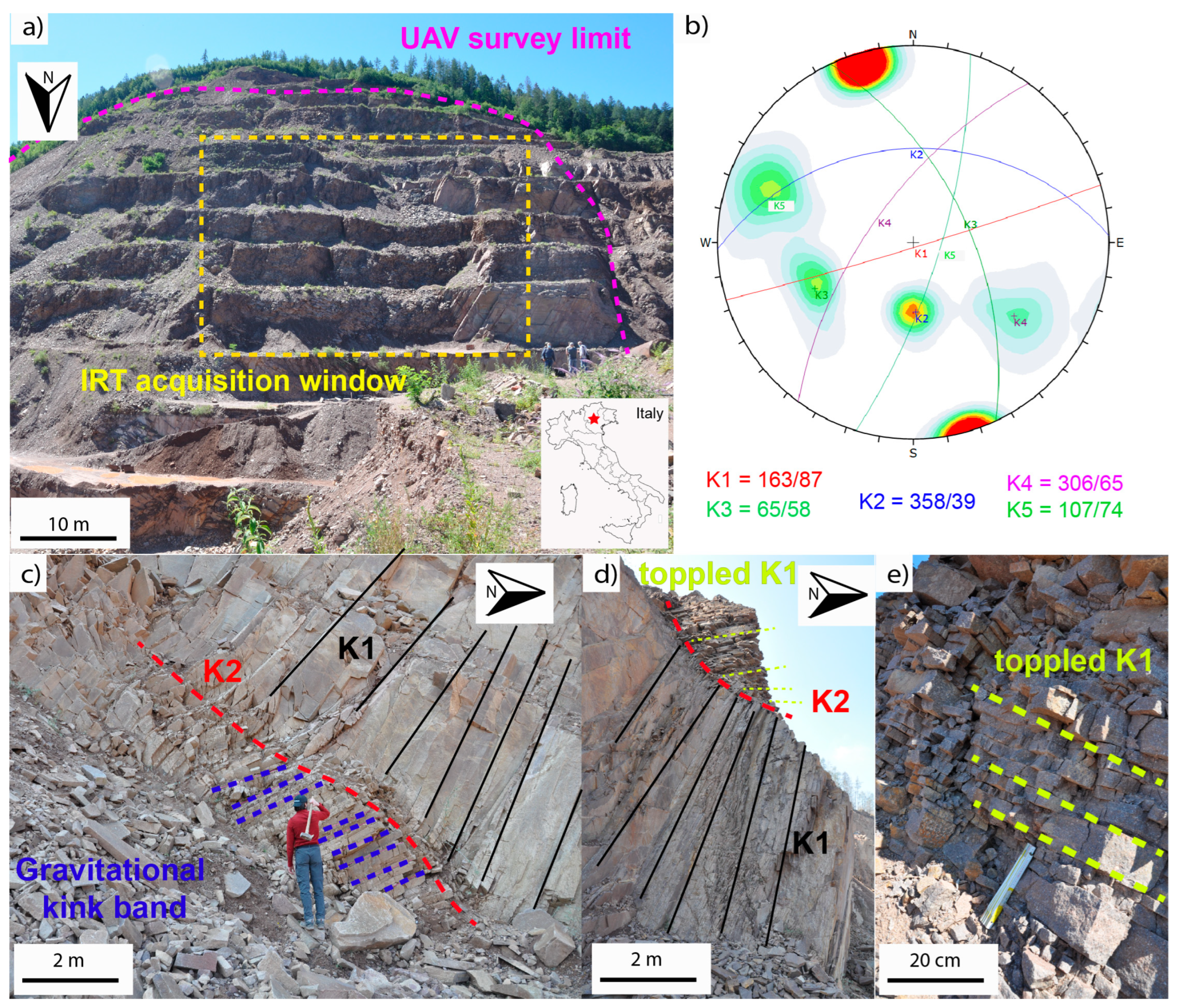
Abstract
:1. Introduction
2. Field Laboratory: Mt. Gorsa Quarry
3. Materials and Methods
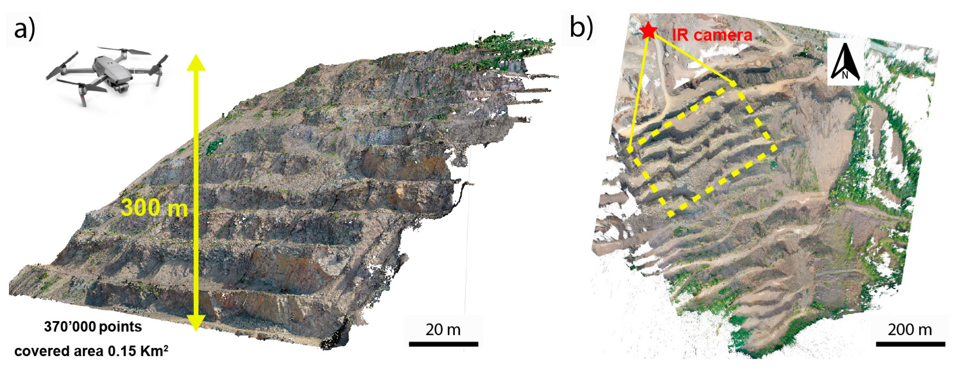
3.1. Three-Dimensional Slope Geometry: UAV Photogrammetry
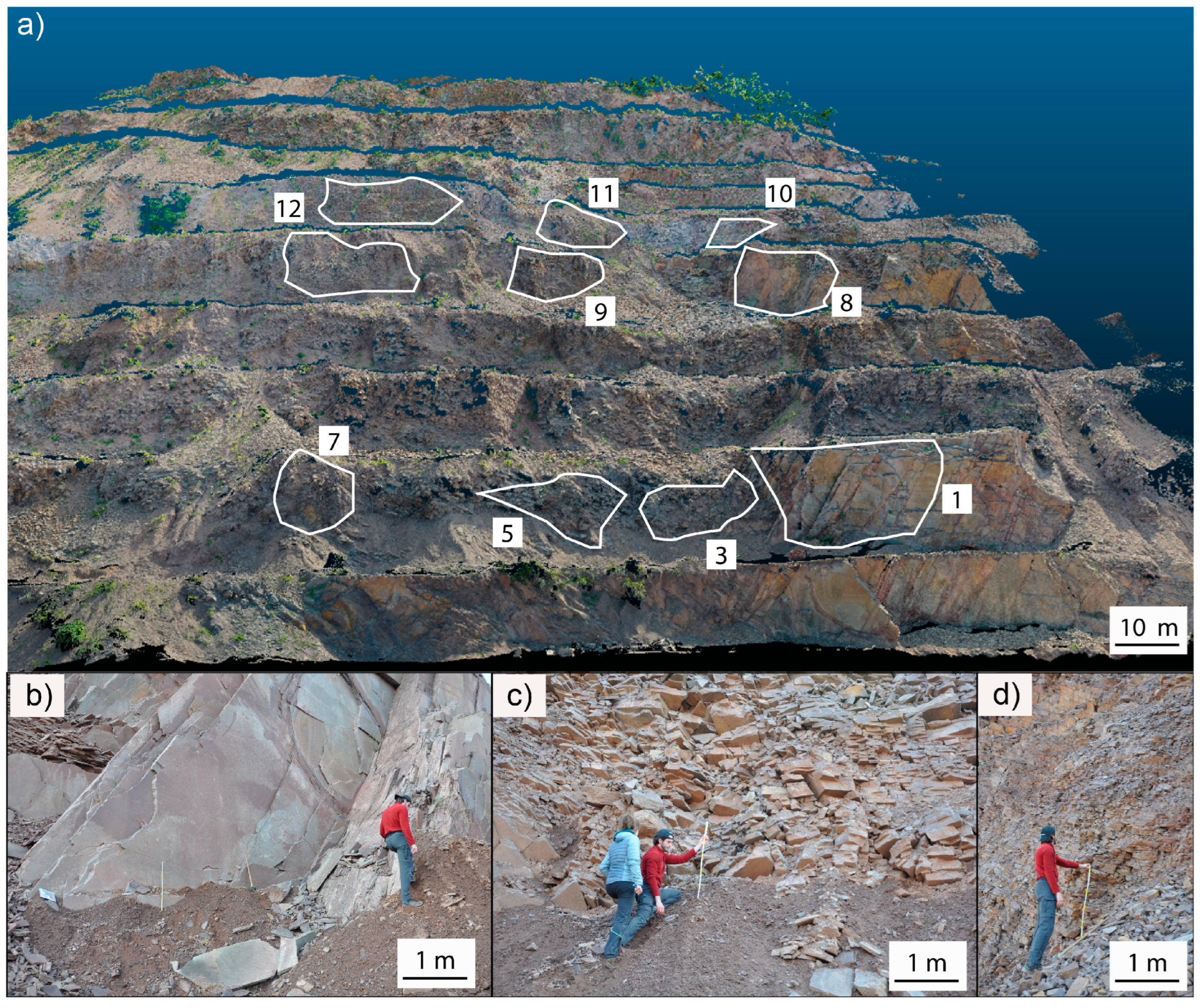
3.2. Rock Mass Quality: Field Characterization
3.3. Rock Mass Thermal Behavior: Infrared Thermography
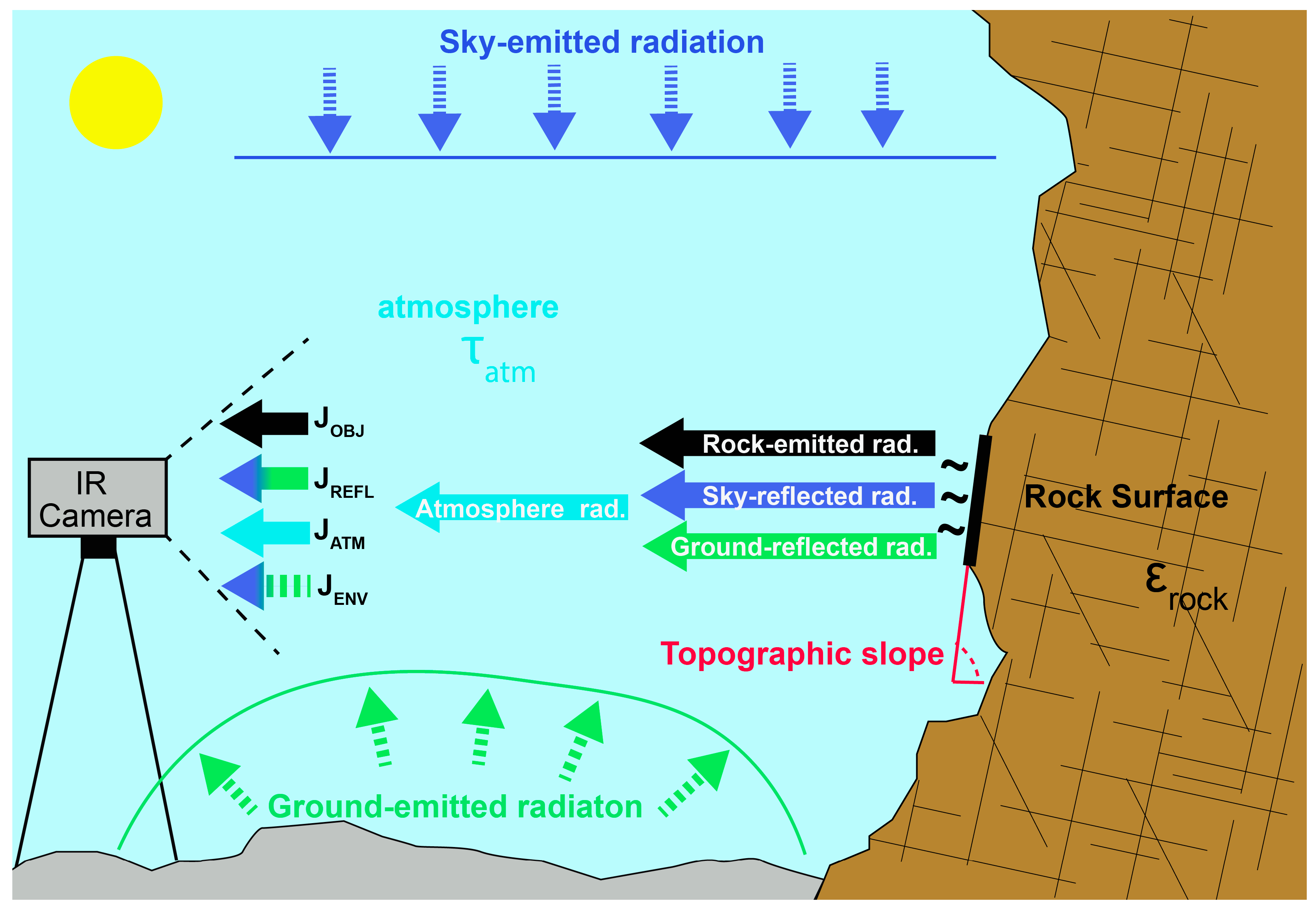
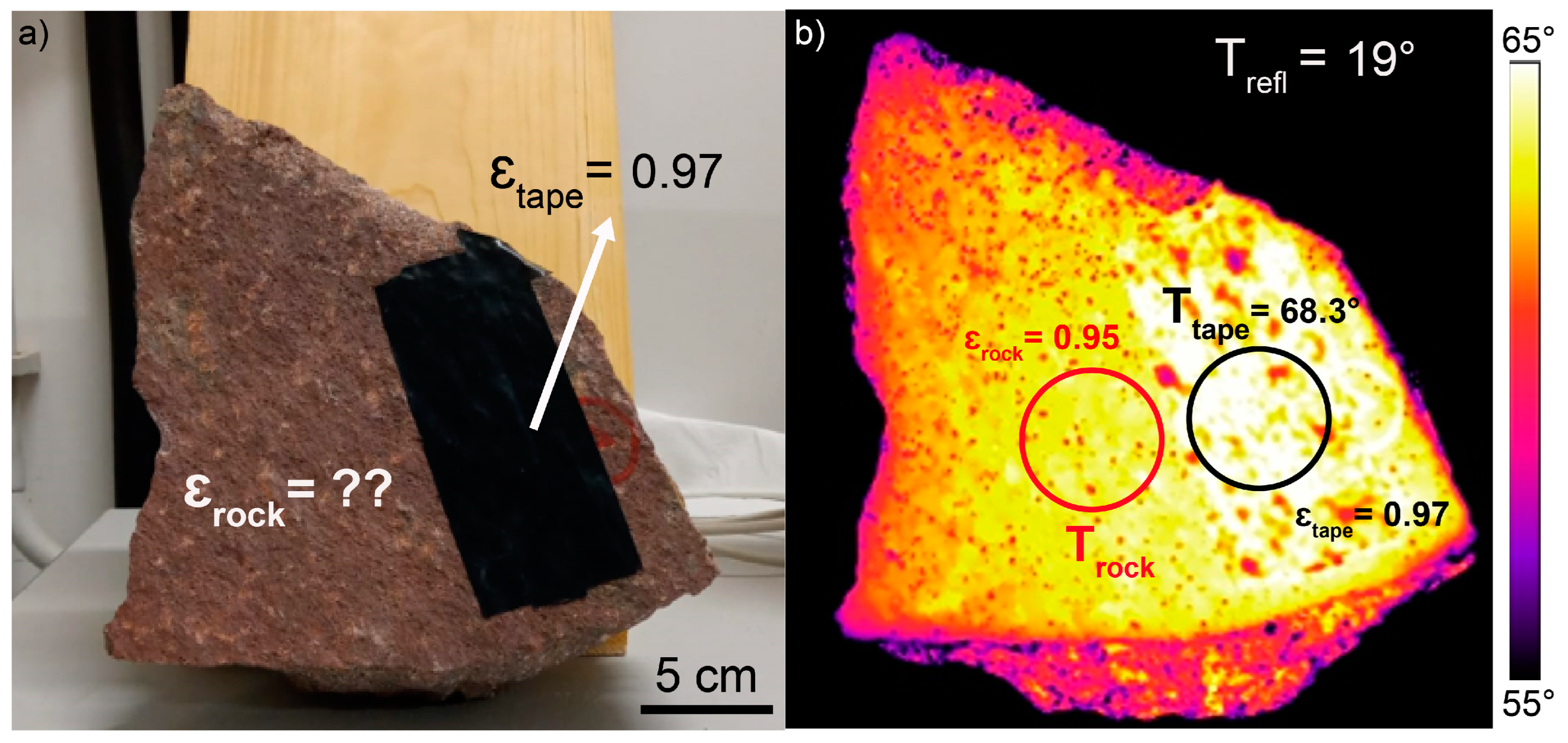
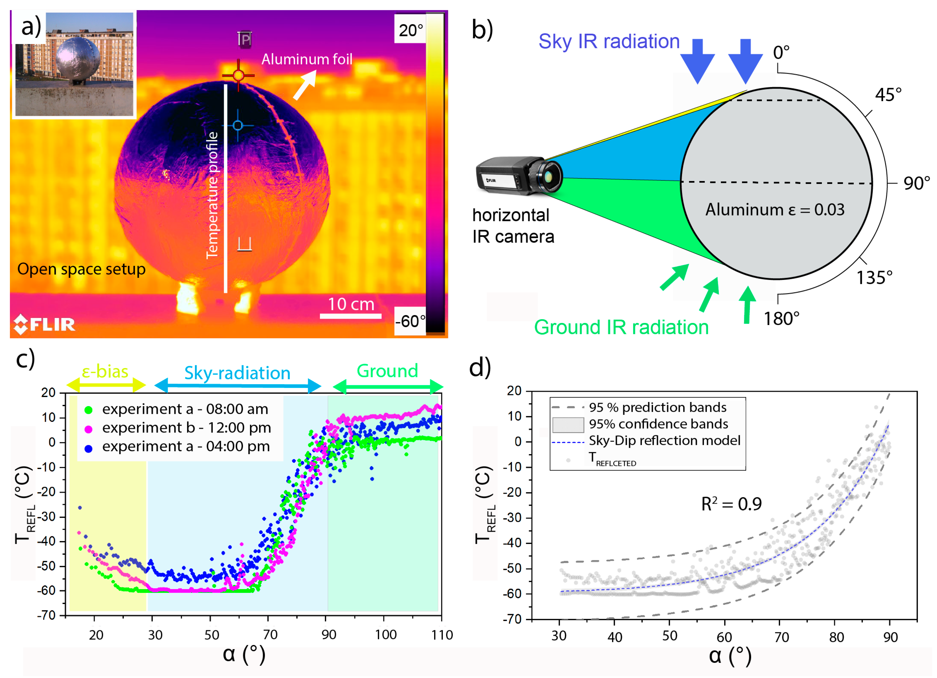
3.3.1. IRT Basics and Environmental Controls

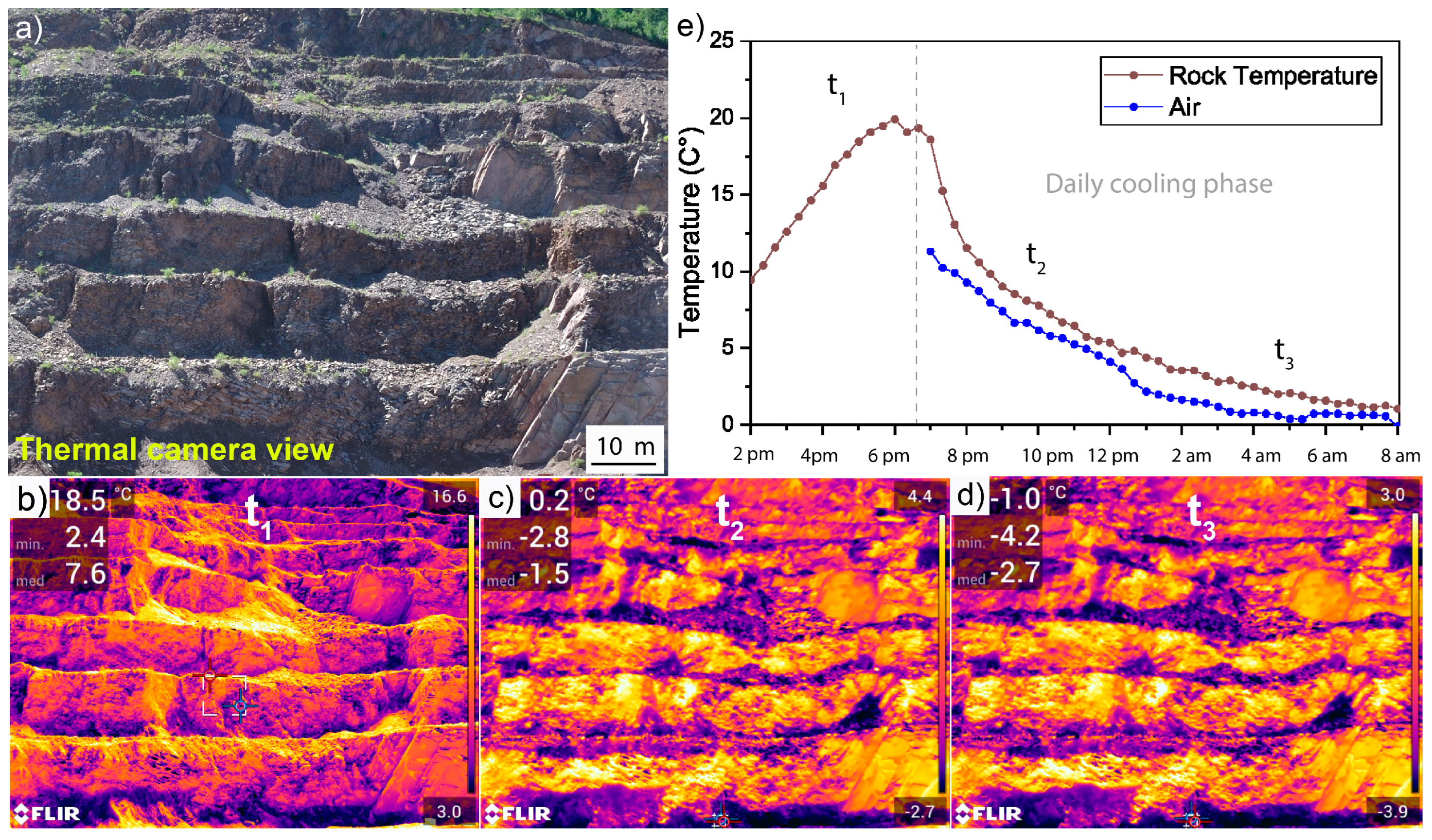
3.3.2. IRT Time-Lapse Survey
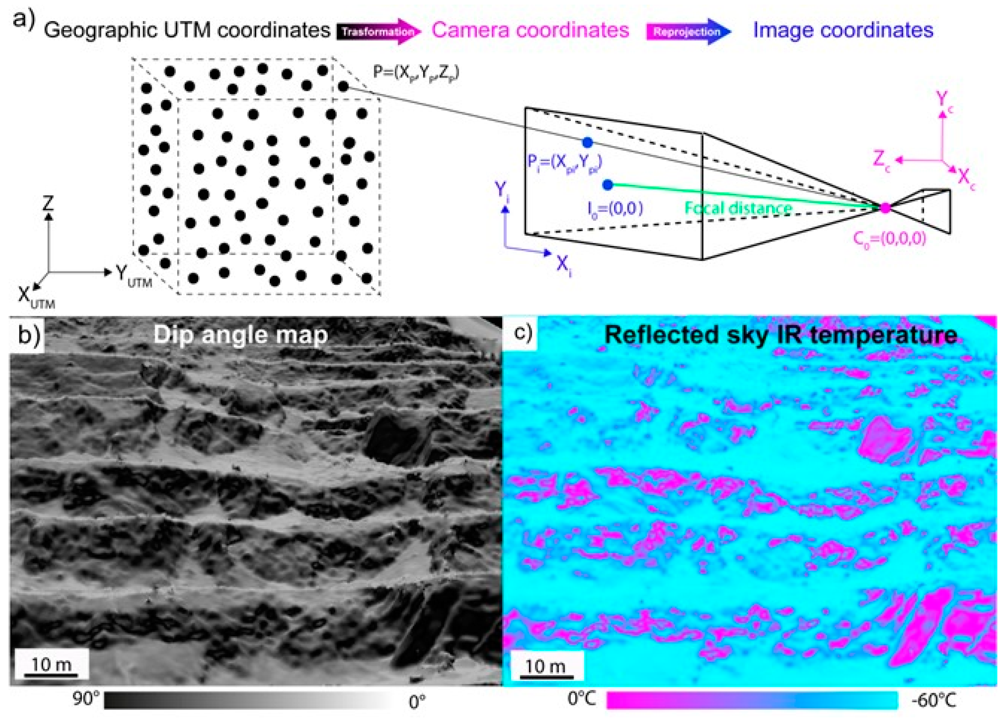
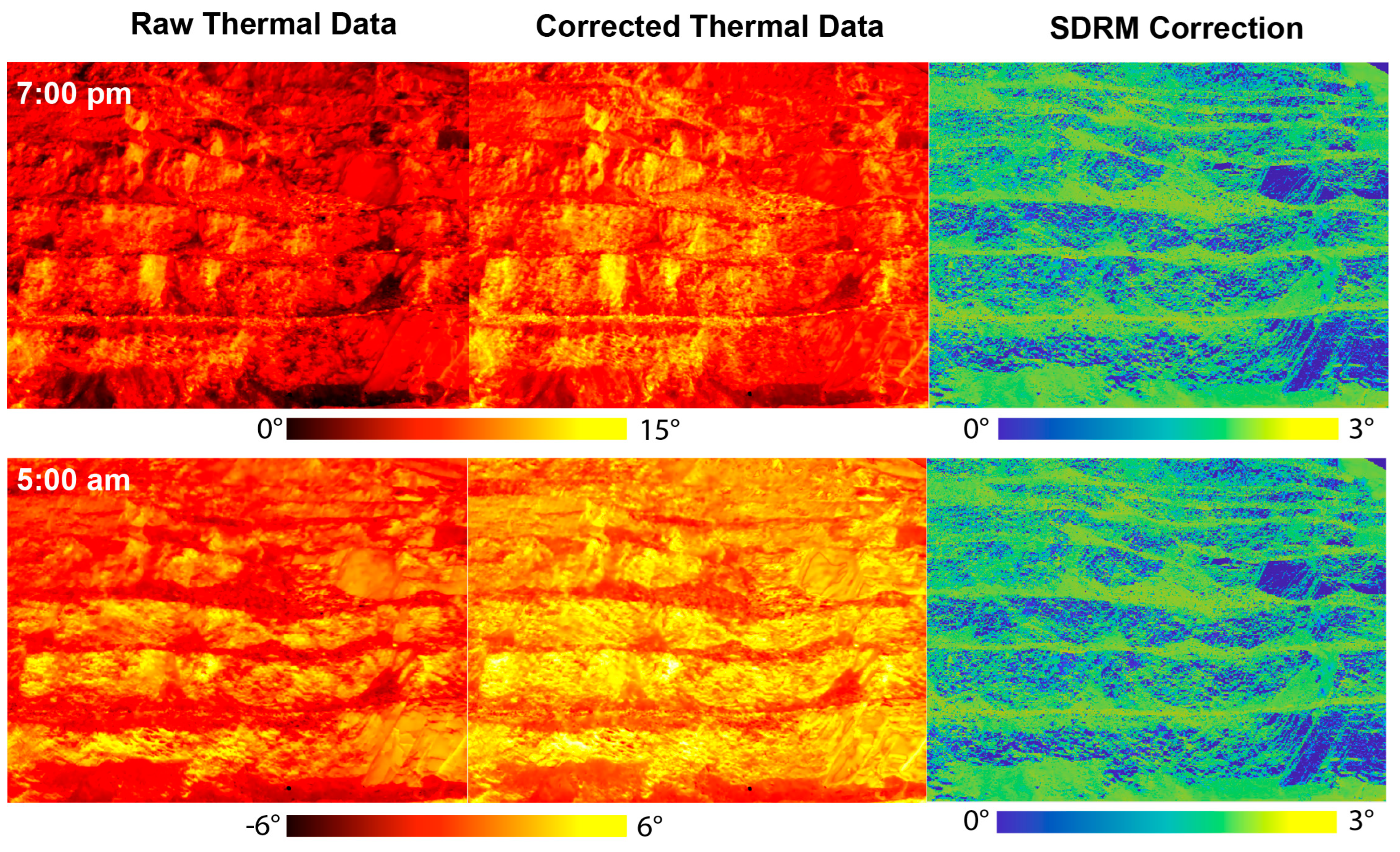
3.3.3. IRT Correction Workflow
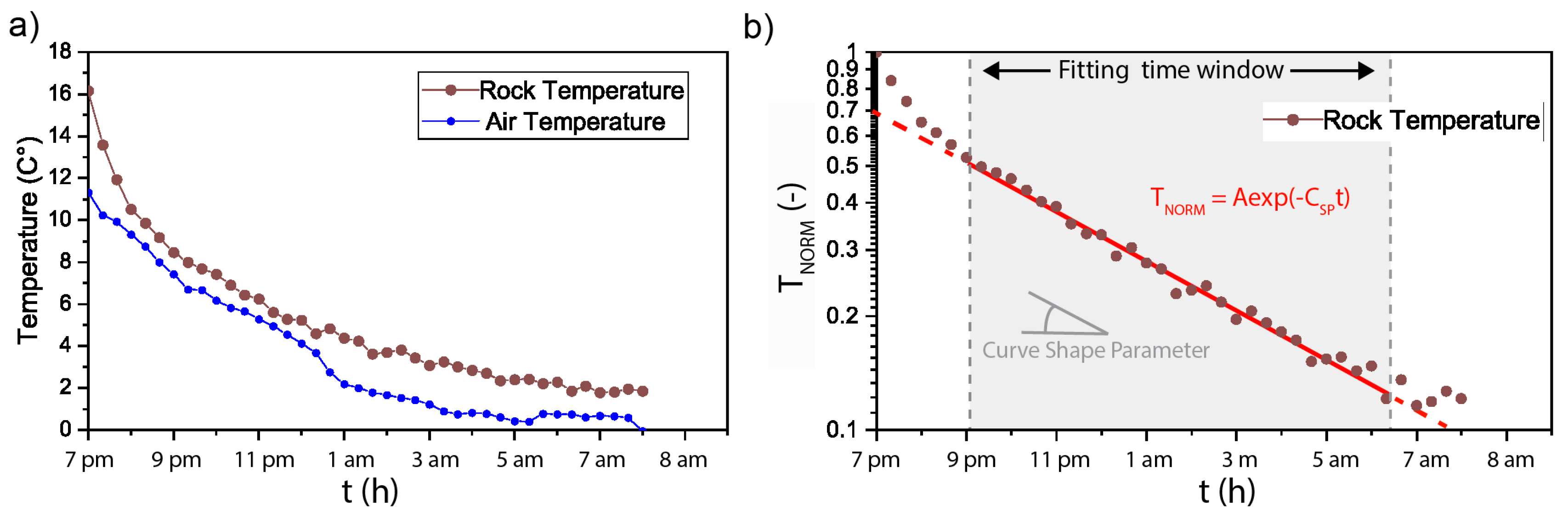
3.4. Rock Mass Cooling Dynamics: Curve Shape Parameter
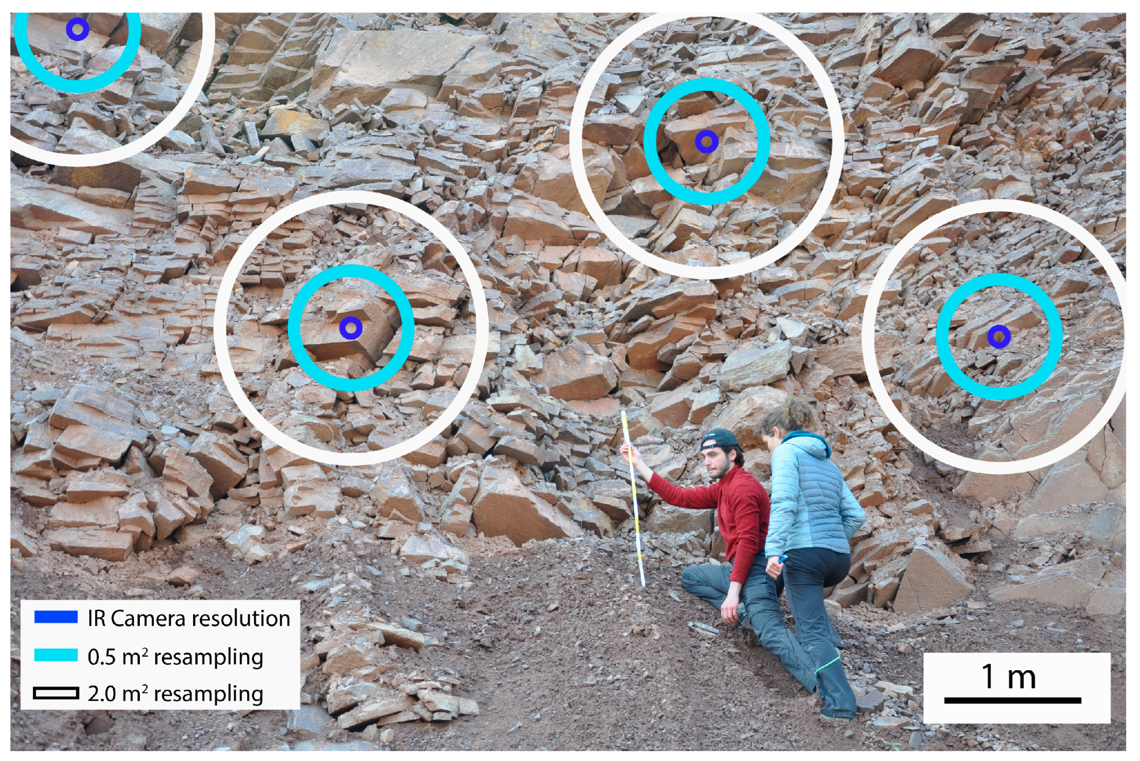
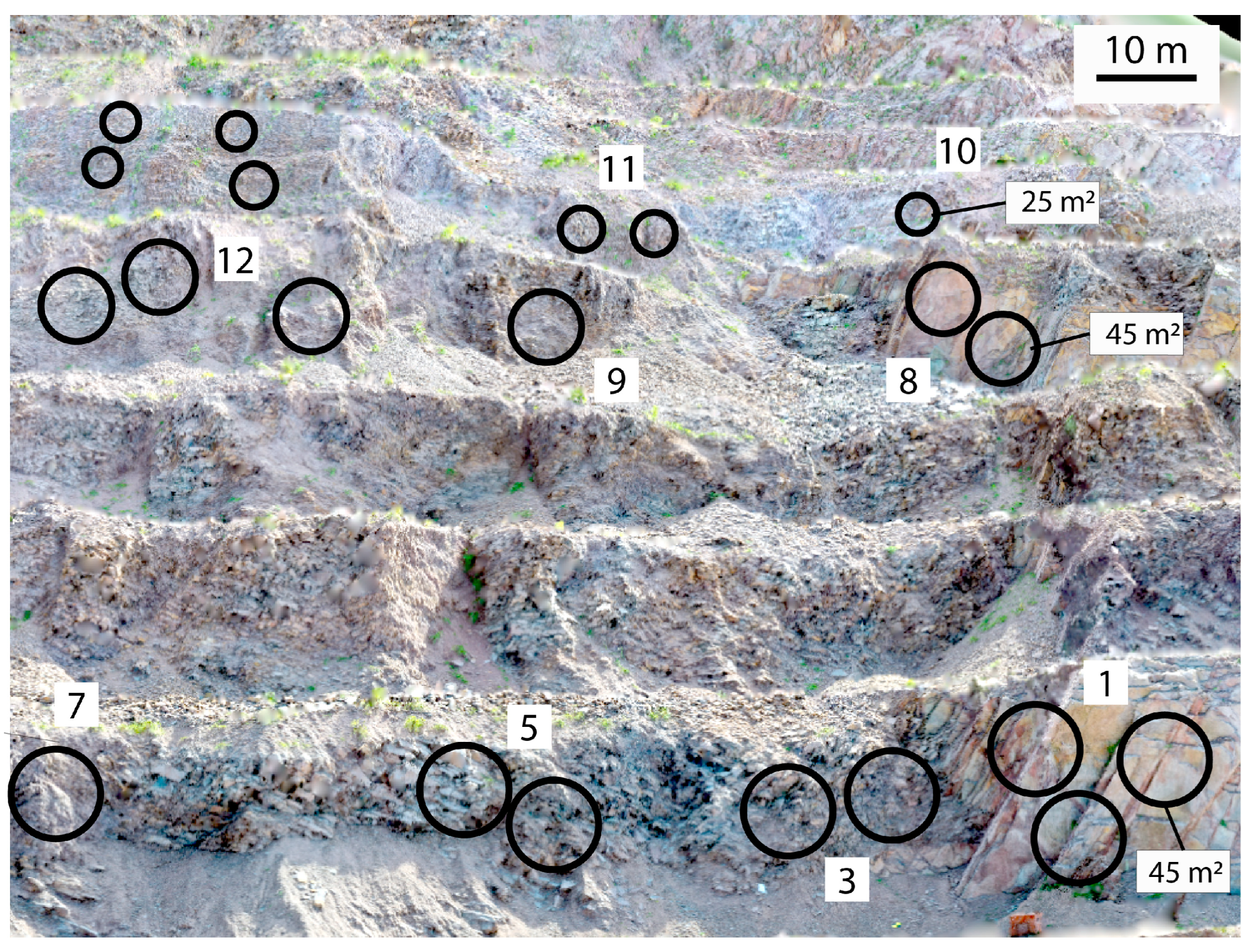
3.5. Distributed Mapping of Rock Mass Quality: CSP-GSI Relationship
4. Results
4.1. Rock Mass Quality: Characteristics and Distribution
4.2. Rock Mass Cooling Dynamics
4.3. GSI-CSP Relationship

4.4. Automated Slope Scale GSI Mapping
5. Discussion and Conclusions
Author Contributions
Funding
Data Availability Statement
Acknowledgments
Conflicts of Interest
References
- Oda, M.; Nemat-Nasser, S.; Konishi, J. Stress-Induced Anisotropy in Granular Masses. Soils Found. 1985, 25, 85–97. [Google Scholar] [CrossRef] [PubMed]
- Hoek, E.; Brown, E.T. Practical Estimates of Rock Mass Strength. Int. J. Rock Mech. Min. Sci. 1997, 34, 1165–1186. [Google Scholar] [CrossRef]
- Hoek, E.; Diederichs, M.S. Empirical Estimation of Rock Mass Modulus. Int. J. Rock Mech. Min. Sci. 2006, 43, 203–215. [Google Scholar] [CrossRef]
- Rutqvist, J.; Rinaldi, A.P.; Cappa, F.; Moridis, G.J. Modeling of Fault Activation and Seismicity by Injection Directly into a Fault Zone Associated with Hydraulic Fracturing of Shale-Gas Reservoirs. J. Pet. Sci. Eng. 2015, 127, 377–386. [Google Scholar] [CrossRef]
- Mandl, G. Rock Joints; Springer: Berlin/Heidelberg, Germany, 2005; ISBN 3540264574. [Google Scholar]
- Watkins, H.; Bond, C.E.; Healy, D.; Butler, R.W.H. Appraisal of Fracture Sampling Methods and a New Workflow to Characterise Heterogeneous Fracture Networks at Outcrop. J. Struct. Geol. 2015, 72, 67–82. [Google Scholar] [CrossRef]
- Bistacchi, A.; Mittempergher, S.; Martinelli, M. Digital Outcrop Model Reconstruction and Interpretation. In 3D Digital Geological Models: From Terrestrial Outcrops to Planetary Surfaces; John Wiley & Sons: Hoboken, NJ, USA, 2022; pp. 11–32. [Google Scholar]
- Savage, H.M.; Brodsky, E.E. Collateral Damage: Evolution with Displacement of Fracture Distribution and Secondary Fault Strands in Fault Damage Zones. J. Geophys. Res. Solid Earth 2011, 116. [Google Scholar] [CrossRef]
- Peacock, D.C.P.; Dimmen, V.; Rotevatn, A.; Sanderson, D.J. A Broader Classification of Damage Zones. J. Struct. Geol. 2017, 102, 179–192. [Google Scholar] [CrossRef]
- Ziegler, M.; Loew, S.; Moore, J.R. Distribution and Inferred Age of Exfoliation Joints in the Aar Granite of the Central Swiss Alps and Relationship to Quaternary Landscape Evolution. Geomorphology 2013, 201, 344–362. [Google Scholar] [CrossRef]
- Eberhardt, E.; Stead, D.; Coggan, J.S. Numerical Analysis of Initiation and Progressive Failure in Natural Rock Slopes—The 1991 Randa Rockslide. Int. J. Rock Mech. Min. Sci. 2004, 41, 69–87. [Google Scholar] [CrossRef]
- Crosta, G.B.; Frattini, P.; Agliardi, F. Deep Seated Gravitational Slope Deformations in the European Alps. Tectonophysics 2013, 605, 13–33. [Google Scholar] [CrossRef]
- Riva, F.; Agliardi, F.; Amitrano, D.; Crosta, G.B. Damage-Based Time-Dependent Modeling of Paraglacial to Postglacial Progressive Failure of Large Rock Slopes. J. Geophys. Res. Earth Surf. 2018, 123, 124–141. [Google Scholar] [CrossRef]
- Spreafico, M.C.; Sternai, P.; Agliardi, F. Paraglacial Rock-Slope Deformations: Sudden or Delayed Response? Insights from an Integrated Numerical Modelling Approach. Landslides 2021, 18, 1311–1326. [Google Scholar] [CrossRef]
- Cai, M.; Kaiser, P.K.; Uno, H.; Tasaka, Y.; Minami, M. Estimation of Rock Mass Deformation Modulus and Strength of Jointed Hard Rock Masses Using the GSI System. Int. J. Rock Mech. Min. Sci. 2004, 41, 3–19. [Google Scholar] [CrossRef]
- Martino, J.B.; Chandler, N.A. Excavation-Induced Damage Studies at the Underground Research Laboratory. Int. J. Rock Mech. Min. Sci. 2004, 41, 1413–1426. [Google Scholar] [CrossRef]
- Pine, R.J.; Harrison, J.P. Rock Mass Properties for Engineering Design. Q. J. Eng. Geol. Hydrogeol. 2003, 36, 5–16. [Google Scholar] [CrossRef]
- Wyllie, D.C.; Mah, C. Rock Slope Engineering; CRC Press: Boca Raton, FL, USA, 2004; ISBN 0415280001. [Google Scholar]
- Brideau, M.-A.; Yan, M.; Stead, D. The Role of Tectonic Damage and Brittle Rock Fracture in the Development of Large Rock Slope Failures. Geomorphology 2009, 103, 30–49. [Google Scholar] [CrossRef]
- Dershowitz, W.; Miller, I. Dual Porosity Fracture Flow and Transport. Geophys. Res. Lett. 1995, 22, 1441–1444. [Google Scholar] [CrossRef]
- Gischig, V.S.; Giardini, D.; Amann, F.; Hertrich, M.; Krietsch, H.; Loew, S.; Maurer, H.; Villiger, L.; Wiemer, S.; Bethmann, F. Hydraulic Stimulation and Fluid Circulation Experiments in Underground Laboratories: Stepping up the Scale towards Engineered Geothermal Systems. Geomech. Energy Environ. 2020, 24, 100175. [Google Scholar] [CrossRef]
- Martinelli, M.; Bistacchi, A.; Mittempergher, S.; Bonneau, F.; Balsamo, F.; Caumon, G.; Meda, M. Damage Zone Characterization Combining Scan-Line and Scan-Area Analysis on a Km-Scale Digital Outcrop Model: The Qala Fault (Gozo). J. Struct. Geol. 2020, 140, 104144. [Google Scholar] [CrossRef]
- Edelbro, C. Evaluation of Rock Mass Strength Criteria. Ph.D. Thesis, Luleå Tekniska Universitet, Luleå, Sweden, 2004. [Google Scholar]
- Dershowitz, W.S.; Herda, H.H. Interpretation of Fracture Spacing and Intensity. In Proceedings of the 33rd US Symposium on Rock Mechanics (USRMS), Santa Fe, NM, USA, 3–5 June 1992. [Google Scholar]
- Jing, L.; Stephansson, O. Fundamentals of Discrete Element Methods for Rock Engineering: Theory and Applications; Elsevier: Amsterdam, The Netherlands, 2007; ISBN 0080551858. [Google Scholar]
- Zhang, L.; Einstein, H.H. Estimating the Mean Trace Length of Rock Discontinuities. Rock Mech. Rock Eng. 1998, 31, 217–235. [Google Scholar] [CrossRef]
- Mauldon, M.; Dunne, W.M.; Rohrbaugh, M.B., Jr. Circular Scanlines and Circular Windows: New Tools for Characterizing the Geometry of Fracture Traces. J. Struct. Geol. 2001, 23, 247–258. [Google Scholar] [CrossRef]
- Barton, N.; Lien, R.; Lunde, J. Engineering Classification of Rock Masses for the Design of Tunnel Support. Rock Mech. 1974, 6, 189–236. [Google Scholar] [CrossRef]
- Palmstrom, A.; Broch, E. Use and Misuse of Rock Mass Classification Systems with Particular Reference to the Q-System. Tunn. Undergr. Space Technol. 2006, 21, 575–593. [Google Scholar] [CrossRef]
- Bieniawski, Z.T. Classification of Rock Masses for Engineering: The RMR System and Future Trends. In Rock Testing and Site Characterization; Elsevier: Amsterdam, The Netherlands, 1993; pp. 553–573. [Google Scholar]
- Marinos, P.; Hoek, E. GSI: A Geologically Friendly Tool for Rock Mass Strength Estimation. In Proceedings of the ISRM International Symposium, Melbourne, Australia, 19–24 November 2000. [Google Scholar]
- Cai, X.; Zhou, Z.; Tan, L.; Zang, H.; Song, Z. Water Saturation Effects on Thermal Infrared Radiation Features of Rock Materials During Deformation and Fracturing. Rock Mech. Rock Eng. 2020, 53, 4839–4856. [Google Scholar] [CrossRef]
- Agliardi, F.; Sapigni, M.; Crosta, G.B. Rock Mass Characterization by High-Resolution Sonic and GSI Borehole Logging. Rock Mech. Rock Eng. 2016, 49, 4303–4318. [Google Scholar] [CrossRef]
- Agliardi, F.; Crosta, G.B.; Meloni, F.; Valle, C.; Rivolta, C. Structurally-Controlled Instability, Damage and Slope Failure in a Porphyry Rock Mass. Tectonophysics 2013, 605, 34–47. [Google Scholar] [CrossRef]
- Li, X.; Chen, Z.; Chen, J.; Zhu, H. Automatic Characterization of Rock Mass Discontinuities Using 3D Point Clouds. Eng. Geol. 2019, 259, 105131. [Google Scholar] [CrossRef]
- Bistacchi, A.; Mittempergher, S.; Martinelli, M.; Storti, F. On a New Robust Workflow for the Statistical and Spatial Analysis of Fracture Data Collected with Scanlines (or the Importance of Stationarity). Solid Earth 2020, 11, 2535–2547. [Google Scholar] [CrossRef]
- Barton, N. Fracture-Induced Seismic Anisotropy When Shearing Is Involved in Production from Fractured Reservoirs. J. Seism. Explor. 2007, 16, 115. [Google Scholar]
- Teza, G.; Marcato, G.; Castelli, E.; Galgaro, A. IRTROCK: A MATLAB Toolbox for Contactless Recognition of Surface and Shallow Weakness of a Rock Cliff by Infrared Thermography. Comput. Geosci. 2012, 45, 109–118. [Google Scholar] [CrossRef]
- Mineo, S.; Pappalardo, G.; Rapisarda, F.; Cubito, A.; Di Maria, G. Integrated Geostructural, Seismic and Infrared Thermography Surveys for the Study of an Unstable Rock Slope in the Peloritani Chain (NE Sicily). Eng. Geol. 2015, 195, 225–235. [Google Scholar] [CrossRef]
- Pappalardo, G.; Mineo, S.; Zampelli, S.P.; Cubito, A.; Calcaterra, D. InfraRed Thermography Proposed for the Estimation of the Cooling Rate Index in the Remote Survey of Rock Masses. Int. J. Rock Mech. Min. Sci. 2016, 83, 182–196. [Google Scholar] [CrossRef]
- Maldague, X. Theory and Practice of Infrared Technology for Nondestructive Testing; John Wiley & Sons: Hoboken, NJ, USA, 2001. [Google Scholar]
- Vollmer, M.; Mollmann, K.P. Advanced Methods in IR Imaging. In Infrared Thermal Imaging: Fundamentals, Research and Applications; John Wiley & Sons: Hoboken, NJ, USA, 2010. [Google Scholar]
- Clark, M.R.; McCann, D.M.; Forde, M.C. Application of Infrared Thermography to the Non-Destructive Testing of Concrete and Masonry Bridges. NDT E Int. 2003, 36, 265–275. [Google Scholar] [CrossRef]
- Ibarra-Castanedo, C.; Sfarra, S.; Klein, M.; Maldague, X. Solar Loading Thermography: Time-Lapsed Thermographic Survey and Advanced Thermographic Signal Processing for the Inspection of Civil Engineering and Cultural Heritage Structures. Infrared Phys. Technol. 2017, 82, 56–74. [Google Scholar] [CrossRef]
- Spampinato, L.; Calvari, S.; Oppenheimer, C.; Boschi, E. Volcano Surveillance Using Infrared Cameras. Earth-Science Rev. 2011, 106, 63–91. [Google Scholar] [CrossRef]
- Moran, M.S. Thermal Infrared Measurement as an Indicator of Plant Ecosystem Health. In Thermal Remote Sensing in Land Surface Processes; CRC Press: Boca Raton, FL, USA, 2004; pp. 256–282. ISBN 0429210515. [Google Scholar]
- Teza, G.; Marcato, G.; Pasuto, A.; Galgaro, A. Integration of Laser Scanning and Thermal Imaging in Monitoring Optimization and Assessment of Rockfall Hazard: A Case History in the Carnic Alps (Northeastern Italy). Nat. Hazards 2015, 76, 1535–1549. [Google Scholar] [CrossRef]
- Frodella, W.; Gigli, G.; Morelli, S.; Lombardi, L.; Casagli, N. Landslide Mapping and Characterization through Infrared Thermography (IRT): Suggestions for a Methodological Approach from Some Case Studies. Remote Sens. 2017, 9, 1281. [Google Scholar] [CrossRef]
- Guerin, A.; Jaboyedoff, M.; Collins, B.D.; Derron, M.H.; Stock, G.M.; Matasci, B.; Boesiger, M.; Lefeuvre, C.; Podladchikov, Y.Y. Detection of Rock Bridges by Infrared Thermal Imaging and Modeling. Sci. Rep. 2019, 9, 13138. [Google Scholar] [CrossRef]
- Song, Z.; Zhang, Q.; Zhang, Y.; Wang, J.; Fan, S.; Zhou, G. Abnormal Precursory Information Analysis of the Infrared Radiation Temperature (IRT) before Sandstone Failure. KSCE J. Civ. Eng. 2021, 25, 4173–4183. [Google Scholar] [CrossRef]
- Mineo, S.; Pappalardo, G. The Use of Infrared Thermography for Porosity Assessment of Intact Rock. Rock Mech. Rock Eng. 2016, 49, 3027–3039. [Google Scholar] [CrossRef]
- Mineo, S.; Pappalardo, G. InfraRed Thermography Presented as an Innovative and Non-Destructive Solution to Quantify Rock Porosity in Laboratory. Int. J. Rock Mech. Min. Sci. 2019, 115, 99–110. [Google Scholar] [CrossRef]
- Mineo, S.; Caliò, D.; Pappalardo, G. UAV-Based Photogrammetry and Infrared Thermography Applied to Rock Mass Survey for Geomechanical Purposes. Remote Sens. 2022, 14, 473. [Google Scholar] [CrossRef]
- Franzosi, F.; Casiraghi, S.; Colombo, R.; Crippa, C.; Agliardi, F. Quantitative Evaluation of the Fracturing State of Crystalline Rocks Using Infrared Thermography. Rock Mech. Rock Eng. 2023, 56, 6337–6355. [Google Scholar] [CrossRef]
- Grechi, G.; Fiorucci, M.; Marmoni, G.M.; Martino, S. 3D Thermal Monitoring of Jointed Rock Masses through Infrared Thermography and Photogrammetry. Remote Sens. 2021, 13, 957. [Google Scholar] [CrossRef]
- Baroň, I.; Bečkovský, D.; Míča, L. Application of Infrared Thermography for Mapping Open Fractures in Deep-Seated Rockslides and Unstable Cliffs. Landslides 2014, 11, 15–27. [Google Scholar] [CrossRef]
- Frodella, W.; Fidolini, F.; Morelli, S.; Pazzi, V. Application of Infrared Thermography for Landslide Mapping: The Rotolon DSGDS Case Study. Rend. Online Soc. Geol. Ital. 2015, 35, 144–147. [Google Scholar] [CrossRef]
- Flir Corporation. User’s Manual FLIR T10xx Series. Available online: https://www.red-current.com/images/User_Manuals/FLIR_T10xx_User_Manual.pdf (accessed on 31 July 2023).
- Minkina, W.; Klecha, D. Atmospheric Transmission Coefficient Modelling in the Infrared for Thermovision Measurements. J. Sensors Sens. Syst. 2016, 5, 17–23. [Google Scholar] [CrossRef]
- Kelsey, V.; Riley, S.; Minschwaner, K. Atmospheric Precipitable Water Vapor and Its Correlation with Clear-Sky Infrared Temperature Observations. Atmos. Meas. Tech. 2022, 15, 1563–1576. [Google Scholar] [CrossRef]
- Rottura, A.; Bargossi, G.M.; Caggianelli, A.; Del Moro, A.; Visona, D.; Tranne, C.A. Origin and Significance of the Permian High-K Calc-Alkaline Magmatism in the Central-Eastern Southern Alps, Italy. Lithos 1998, 45, 329–348. [Google Scholar] [CrossRef]
- ISPRA. Carta Geologica d’Italia—1:50.000 Progetto CARG: Modifiche Ed Integrazioni Al Quaderno n. 1/1992. Serv. Geol. d’Italia Quad. Ser. III 2009, 12. Available online: https://www.isprambiente.gov.it/contentfiles/00002800/2880-q12-fasc-iii.pdf (accessed on 31 July 2023).
- Hoek, E.; Marinos, P.; Benissi, M. Applicability of the Geological Strength Index (GSI) Classification for Very Weak and Sheared Rock Masses. The Case of the Athens Schist Formation. Bull. Eng. Geol. Environ. 1998, 57, 151–160. [Google Scholar] [CrossRef]
- Hoek, E.; Brown, E.T. The Hoek–Brown Failure Criterion and GSI–2018 Edition. J. Rock Mech. Geotech. Eng. 2019, 11, 445–463. [Google Scholar] [CrossRef]
- Westoby, M.J.; Brasington, J.; Glasser, N.F.; Hambrey, M.J.; Reynolds, J.M. ‘Structure-from-Motion’Photogrammetry: A Low-Cost, Effective Tool for Geoscience Applications. Geomorphology 2012, 179, 300–314. [Google Scholar] [CrossRef]
- Wilkinson, M.W.; Jones, R.R.; Woods, C.E.; Gilment, S.R.; McCaffrey, K.J.W.; Kokkalas, S.; Long, J.J. A Comparison of Terrestrial Laser Scanning and Structure-from-Motion Photogrammetry as Methods for Digital Outcrop Acquisition. Geosphere 2016, 12, 1865–1880. [Google Scholar] [CrossRef]
- Francioni, M.; Simone, M.; Stead, D.; Sciarra, N.; Mataloni, G.; Calamita, F. A New Fast and Low-Cost Photogrammetry Method for the Engineering Characterization of Rock Slopes. Remote Sens. 2019, 11, 1267. [Google Scholar] [CrossRef]
- International Society for Rock Mechanics Commission on Standardization of Laboratory and Field Tests: Suggested Methods for the Quantitative Description of Discontinuities in Rock Masses. Int. J. Rock Mech. Min. Sci. Geomech. Abstr. 1978, 15, 319–368. [CrossRef]
- Vollmer, M.; Möllmann, K.-P. Fundamental of Infrared Thermal Imaging. In An Automated Irrigation System Using Arduino Microcontroller; John Wiley & Sons: Hoboken, NJ, USA, 2018; pp. 2–6. ISBN 9781493990047. [Google Scholar]
- Hillel, D. Environmental Soil Physics: Fundamentals, Applications, and Environmental Considerations; Elsevier Science: Amsterdam, The Netherlands, 2014; ISBN 0080544150. [Google Scholar]
- Fiorucci, M.; Marmoni, G.M.; Martino, S.; Mazzanti, P. Thermal Response of Jointed Rock Masses Inferred from Infrared Thermographic Surveying (Acuto Test-Site, Italy). Sensors 2018, 18, 2221. [Google Scholar] [CrossRef]
- Mineo, S.; Pappalardo, G. Rock Emissivity Measurement for Infrared Thermography Engineering Geological Applications. Appl. Sci. 2021, 11, 3773. [Google Scholar] [CrossRef]
- Shannon, H.R.; Sigda, J.M.; Van Dam, R.L.; Hendrickx, J.M.H.; McLemore, V.T. Thermal Camera Imaging of Rock Piles at the Questa Molybdenum Mine, Questa, New Mexico. In Proceedings of the 2005 National Meeting of the American Society of Mining and Reclamation, Breckenridge, CO, USA, 19–23 June 2005. [Google Scholar]
- Sass, O.; Bauer, C.; Fruhmann, S.; Harald, S.; Kropf, F.; Gaisberger, C. Infrared Thermography Monitoring of Rock Faces Potential and Pitfalls. Geomorphology 2023, 439, 108837. [Google Scholar] [CrossRef]
- Martin, M.; Berdahl, P. Characteristics of Infrared Sky Radiation in the United States. Sol. Energy 1984, 33, 321–336. [Google Scholar] [CrossRef]
- Howell, I. Fabrication of High Refractive Index, Periodic, Composite Nanostructures for Photonic and Sensing Applications. Ph.D. Thesis, University of Massachusetts Amherst, Amherst, MA, USA, 2018. [Google Scholar]
- Ferreira, R.A.M.; Pottie, D.L.; Dias, L.H.C.; Filho, B.J.C.; Porto, M.P. A Directional-Spectral Approach to Estimate Temperature of Outdoor PV Panels. Sol. Energy 2019, 183, 782–790. [Google Scholar] [CrossRef]
- Agisoft LLC. Photoscan Professional Edition; Agisoft: St. Petersbg, FL, USA, 2018. [Google Scholar]
- Vollmer, M. Newton’s Law of Cooling Revisited. Eur. J. Phys. 2009, 30, 1063. [Google Scholar] [CrossRef]
- Bergman, T.L.; Bergman, T.L.; Incropera, F.P.; Dewitt, D.P.; Lavine, A.S. Fundamentals of Heat and Mass Transfer; John Wiley & Sons: Hoboken, NJ, USA, 2011; ISBN 0470501979. [Google Scholar]
- Turkey, J.W. Exploratory Data Analysis; Pearson: London, UK, 1977; Volume 2. [Google Scholar]
- Whaley, D.L., III. The Interquartile Range: Theory and Estimation. Master’s Thesis, East Tennessee State University, Johnson City, TN, USA, 2005. [Google Scholar]


Disclaimer/Publisher’s Note: The statements, opinions and data contained in all publications are solely those of the individual author(s) and contributor(s) and not of MDPI and/or the editor(s). MDPI and/or the editor(s) disclaim responsibility for any injury to people or property resulting from any ideas, methods, instructions or products referred to in the content. |
© 2023 by the authors. Licensee MDPI, Basel, Switzerland. This article is an open access article distributed under the terms and conditions of the Creative Commons Attribution (CC BY) license (https://creativecommons.org/licenses/by/4.0/).
Share and Cite
Franzosi, F.; Crippa, C.; Derron, M.-H.; Jaboyedoff, M.; Agliardi, F. Slope-Scale Remote Mapping of Rock Mass Fracturing by Modeling Cooling Trends Derived from Infrared Thermography. Remote Sens. 2023, 15, 4525. https://doi.org/10.3390/rs15184525
Franzosi F, Crippa C, Derron M-H, Jaboyedoff M, Agliardi F. Slope-Scale Remote Mapping of Rock Mass Fracturing by Modeling Cooling Trends Derived from Infrared Thermography. Remote Sensing. 2023; 15(18):4525. https://doi.org/10.3390/rs15184525
Chicago/Turabian StyleFranzosi, Federico, Chiara Crippa, Marc-Henri Derron, Michel Jaboyedoff, and Federico Agliardi. 2023. "Slope-Scale Remote Mapping of Rock Mass Fracturing by Modeling Cooling Trends Derived from Infrared Thermography" Remote Sensing 15, no. 18: 4525. https://doi.org/10.3390/rs15184525