
Assessing the Hazard of Deep-Seated Rock Slope Instability through the Description of Potential Failure Scenarios, Cross-Validated Using Several Remote Sensing and Monitoring Techniques


 ,
,
Abstract
: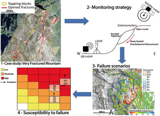
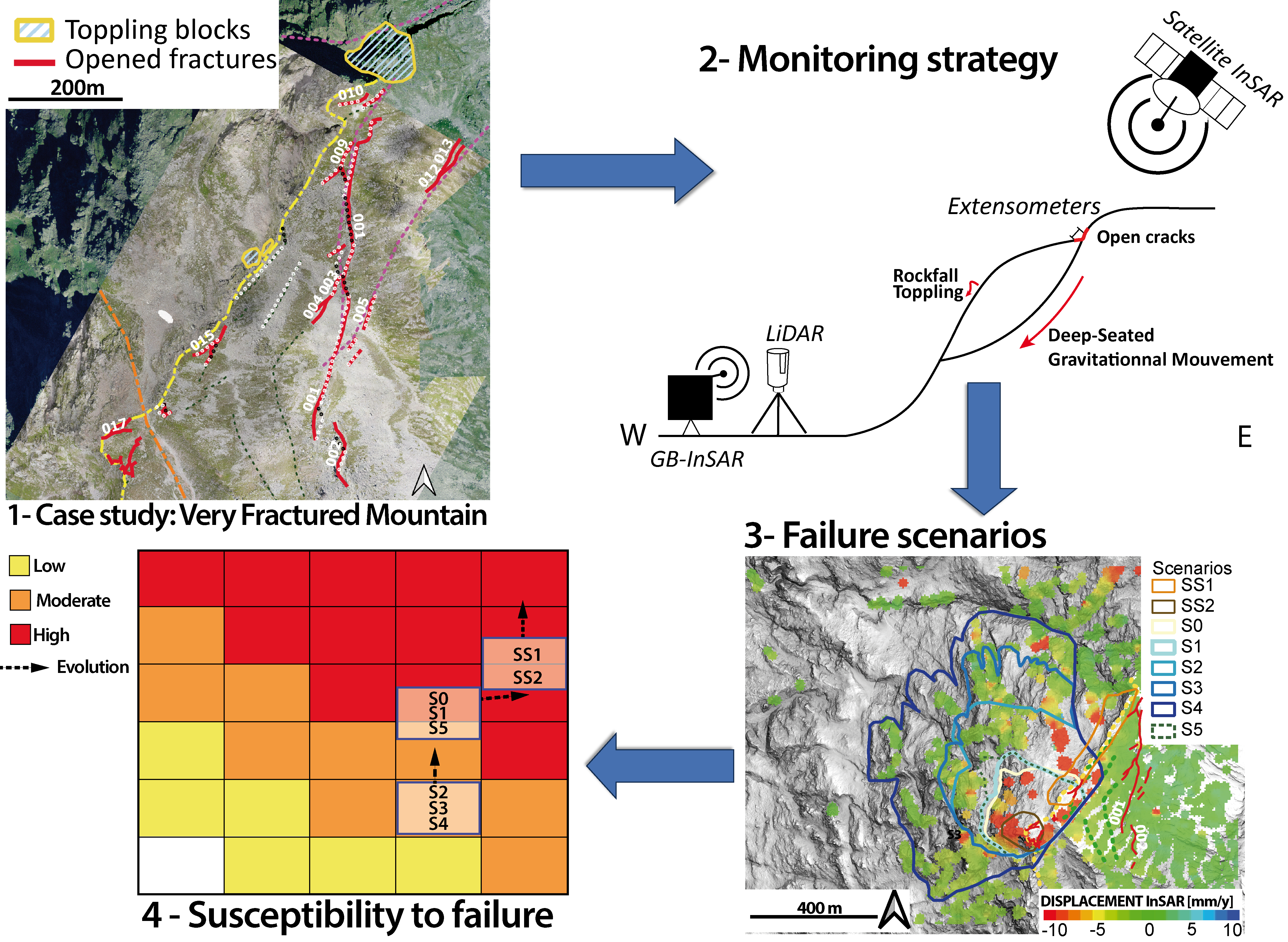
1. Introduction
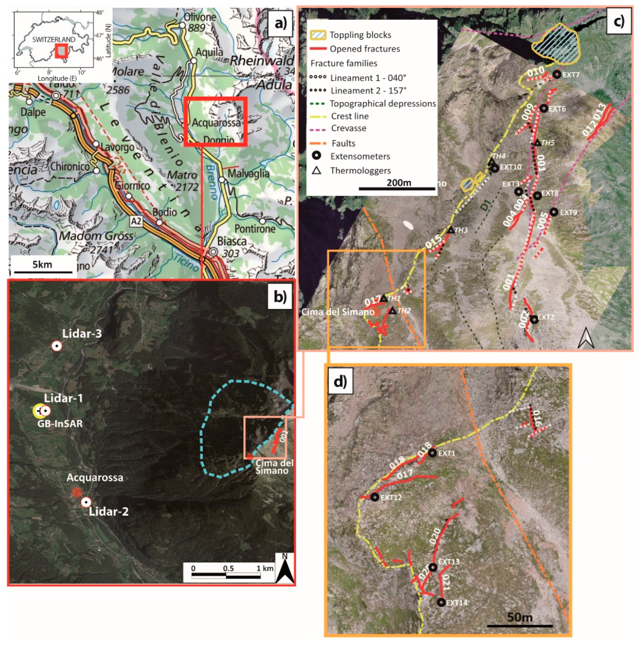
2. Description of Case Study
3. Materials and Methods
3.1. Material and Monitoring
3.1.1. Drone Photogrammetry
3.1.2. Terrestrial LiDAR and High-Precision Panorama
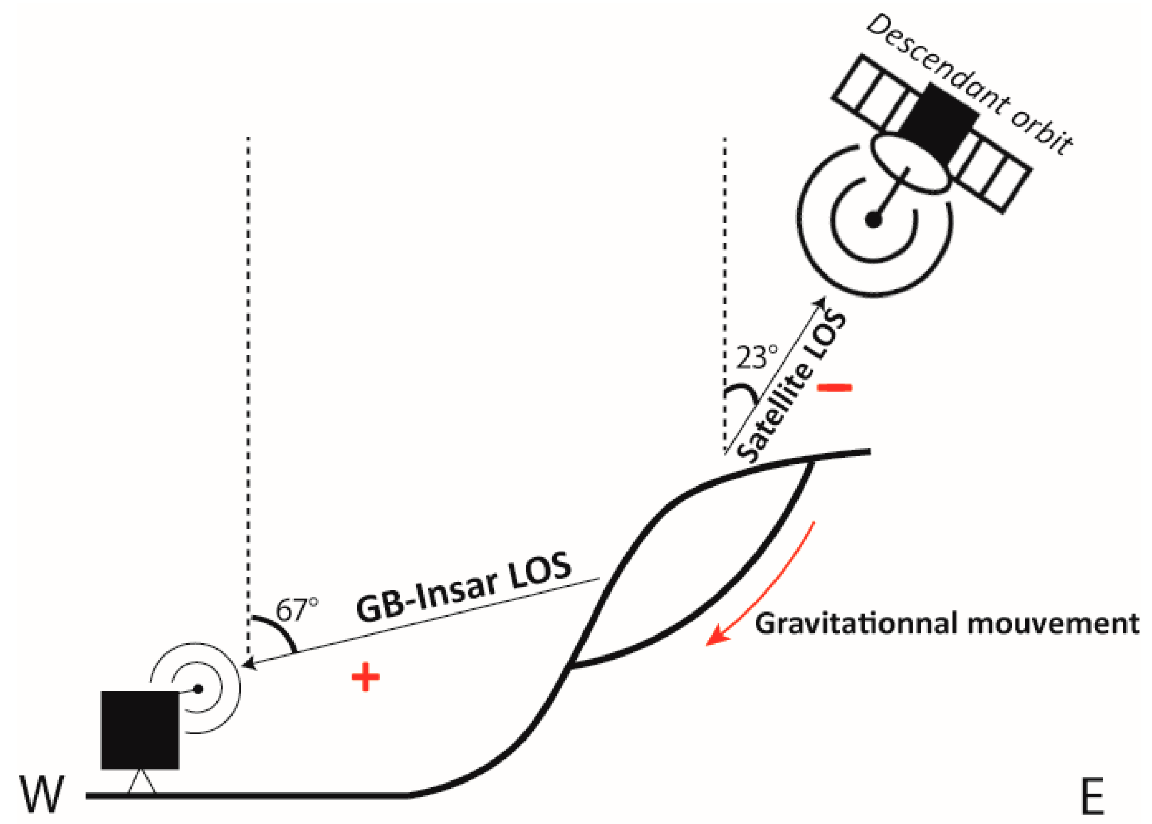
3.1.3. InSAR
Satellite InSAR
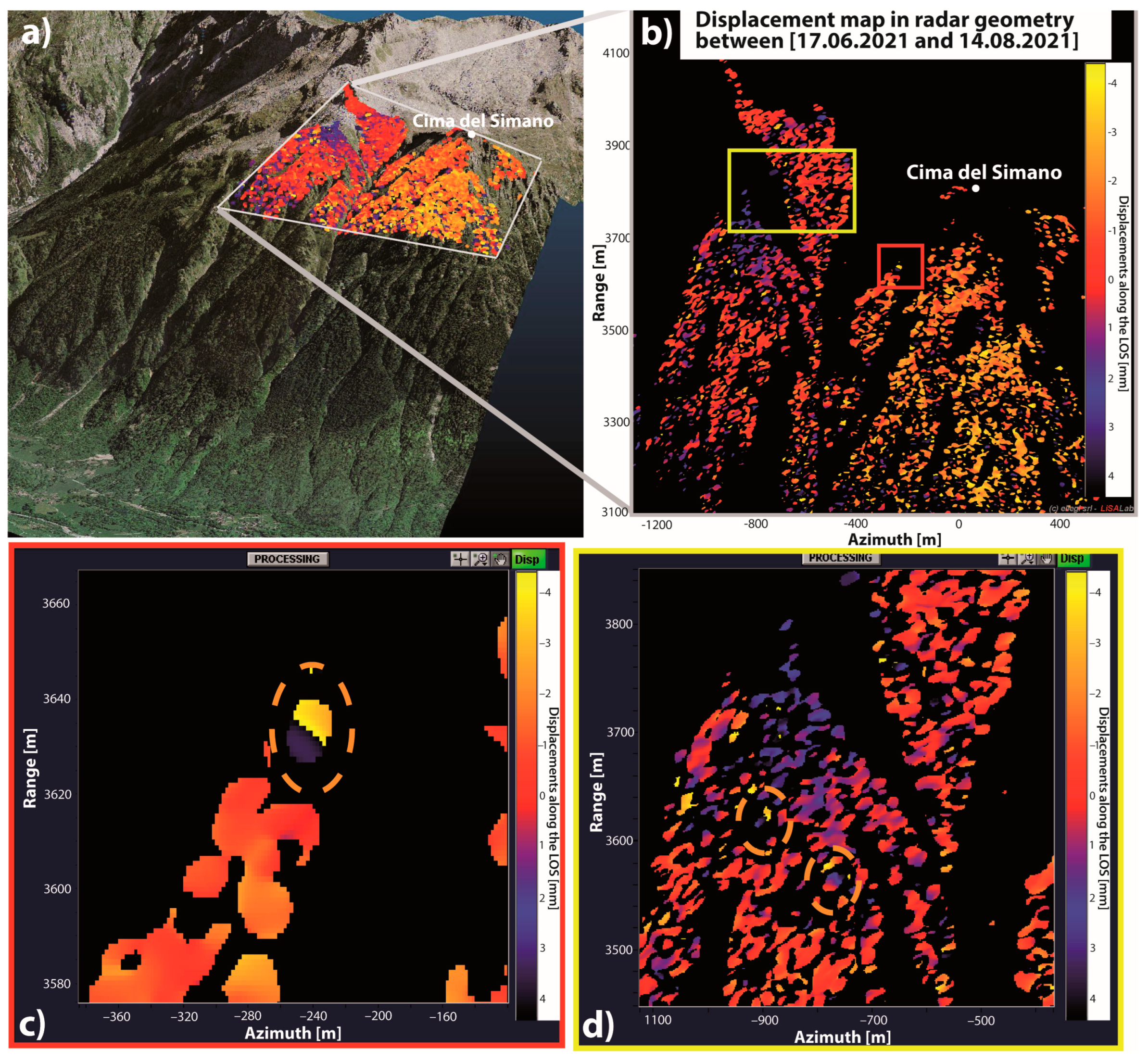
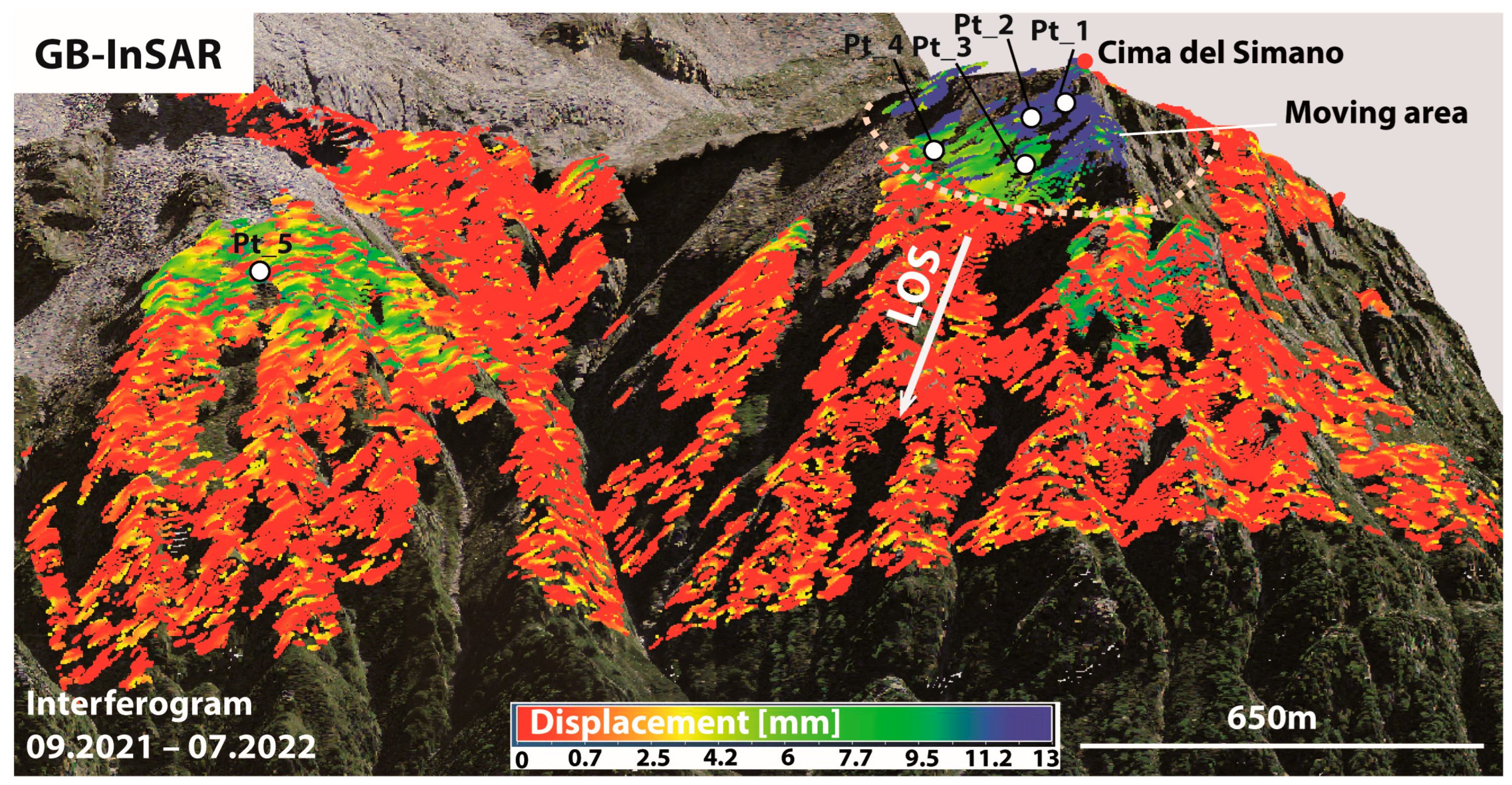
GB-InSAR
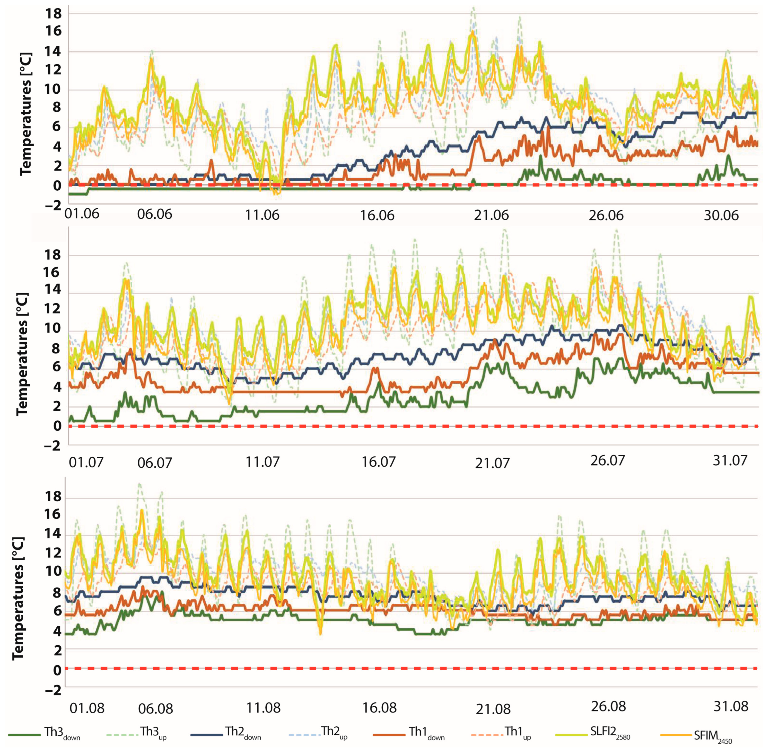
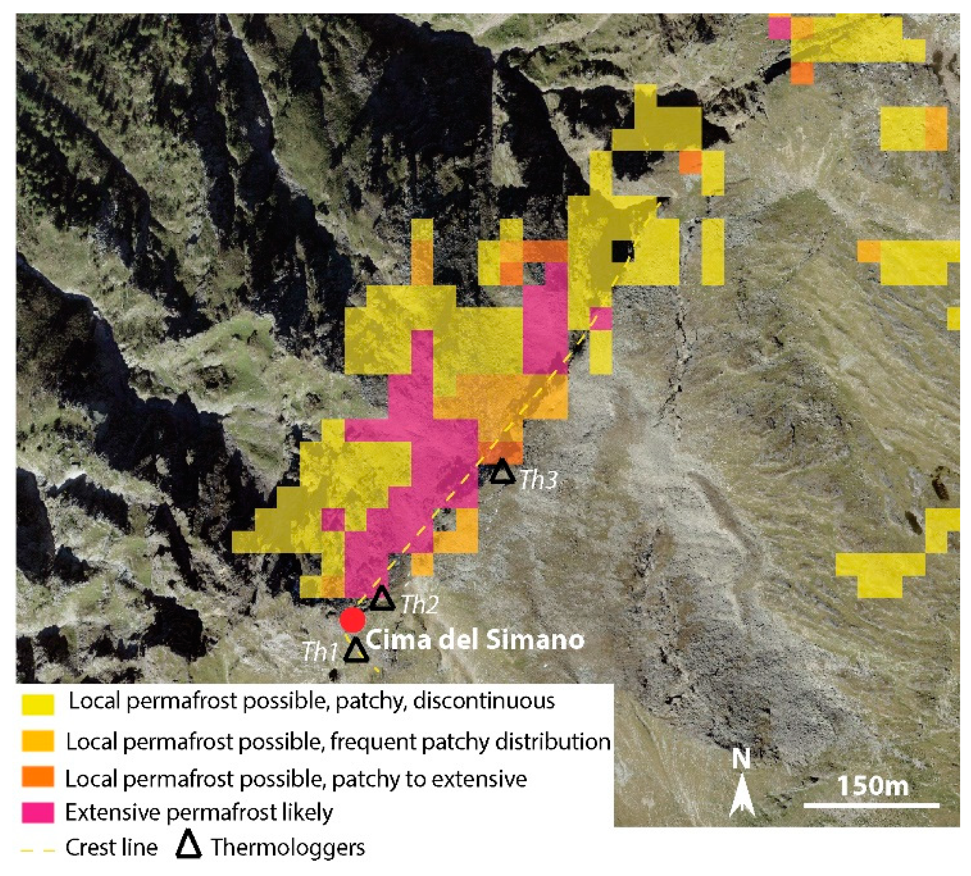
3.1.4. Temperature Monitoring
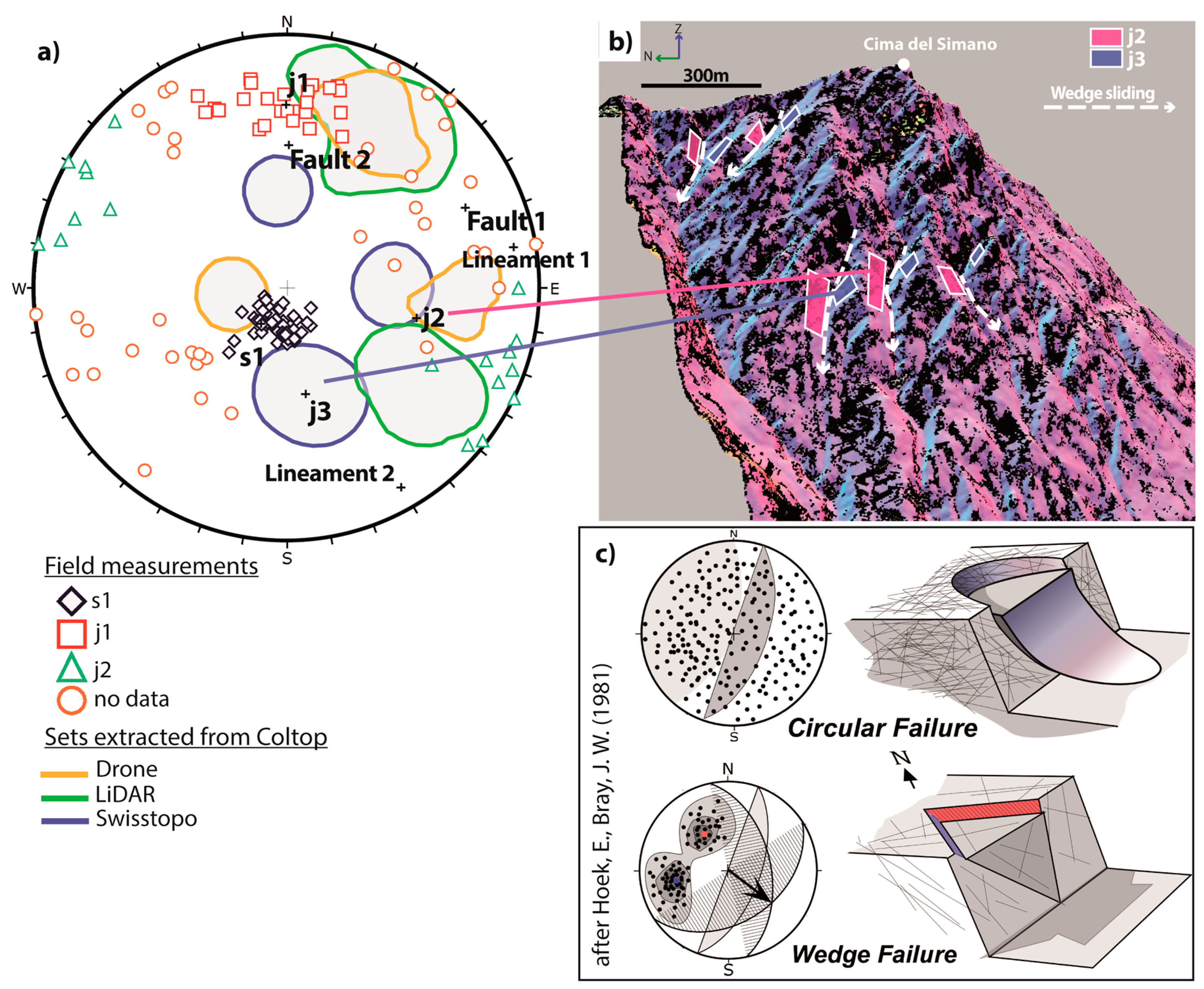
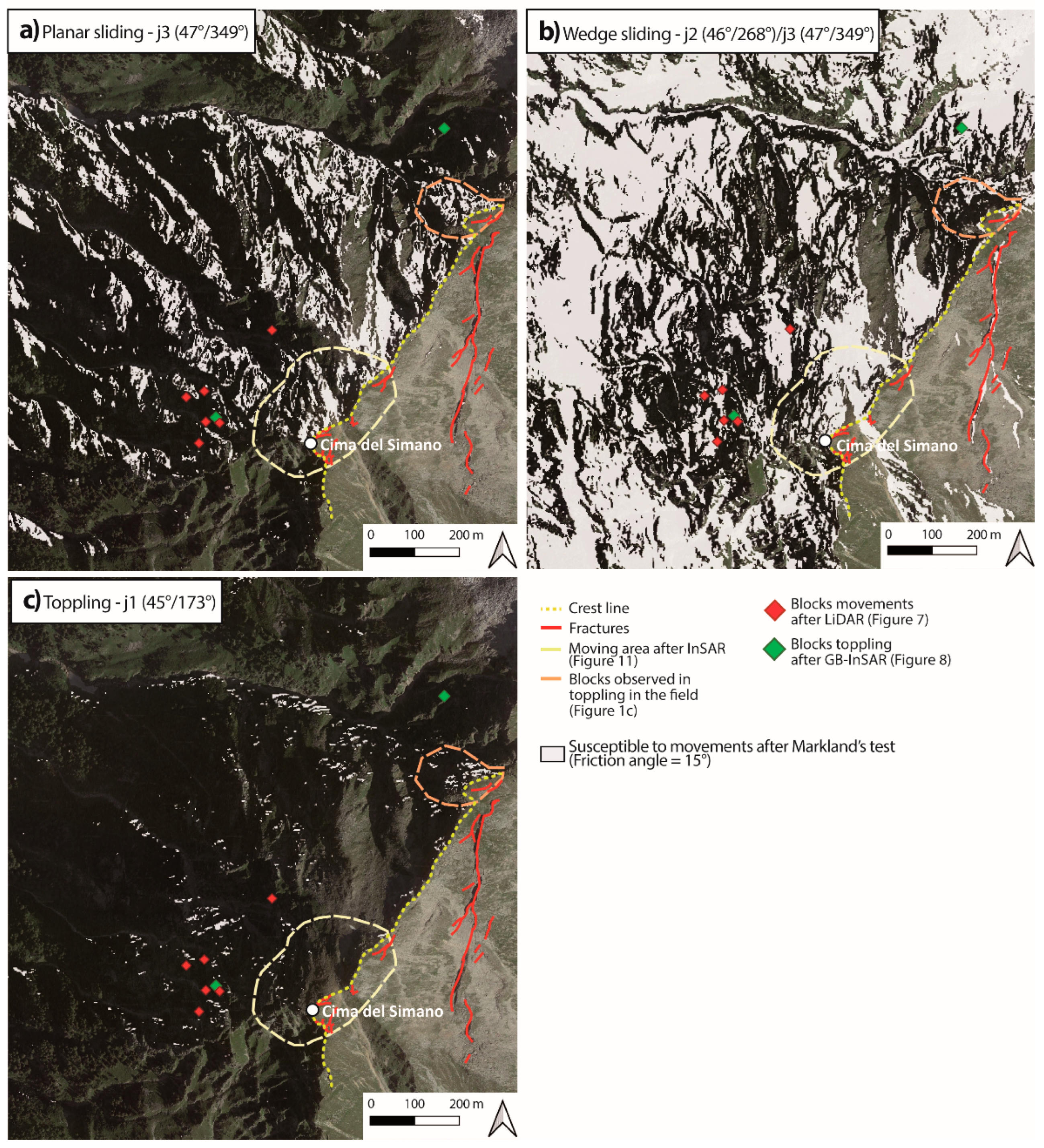
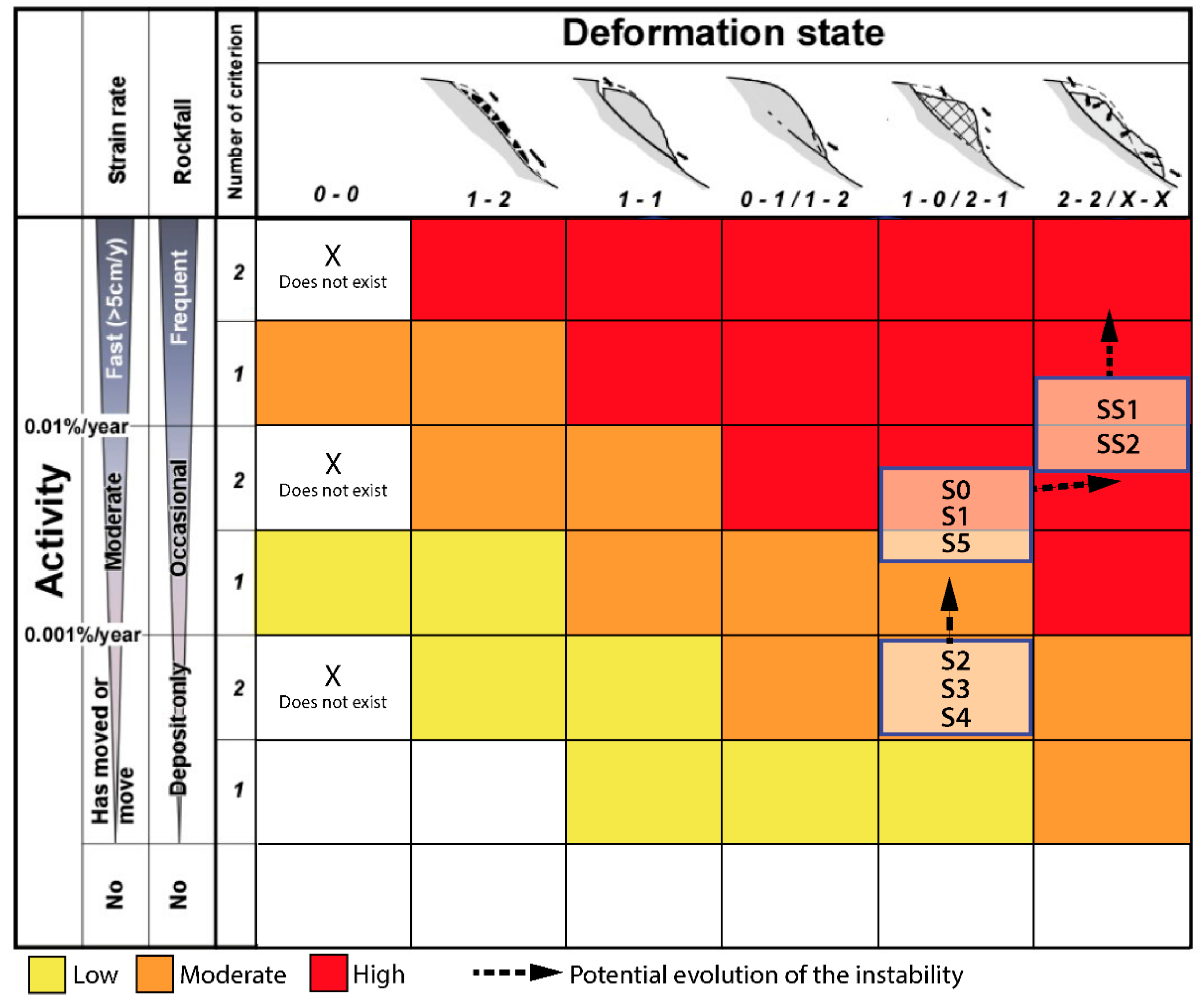
3.2. Structural Analysis and Rupture Scenarios
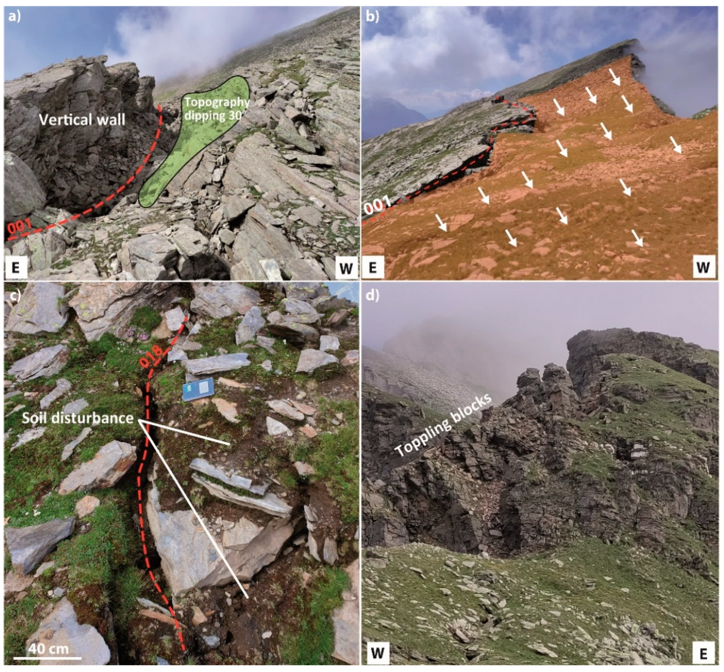
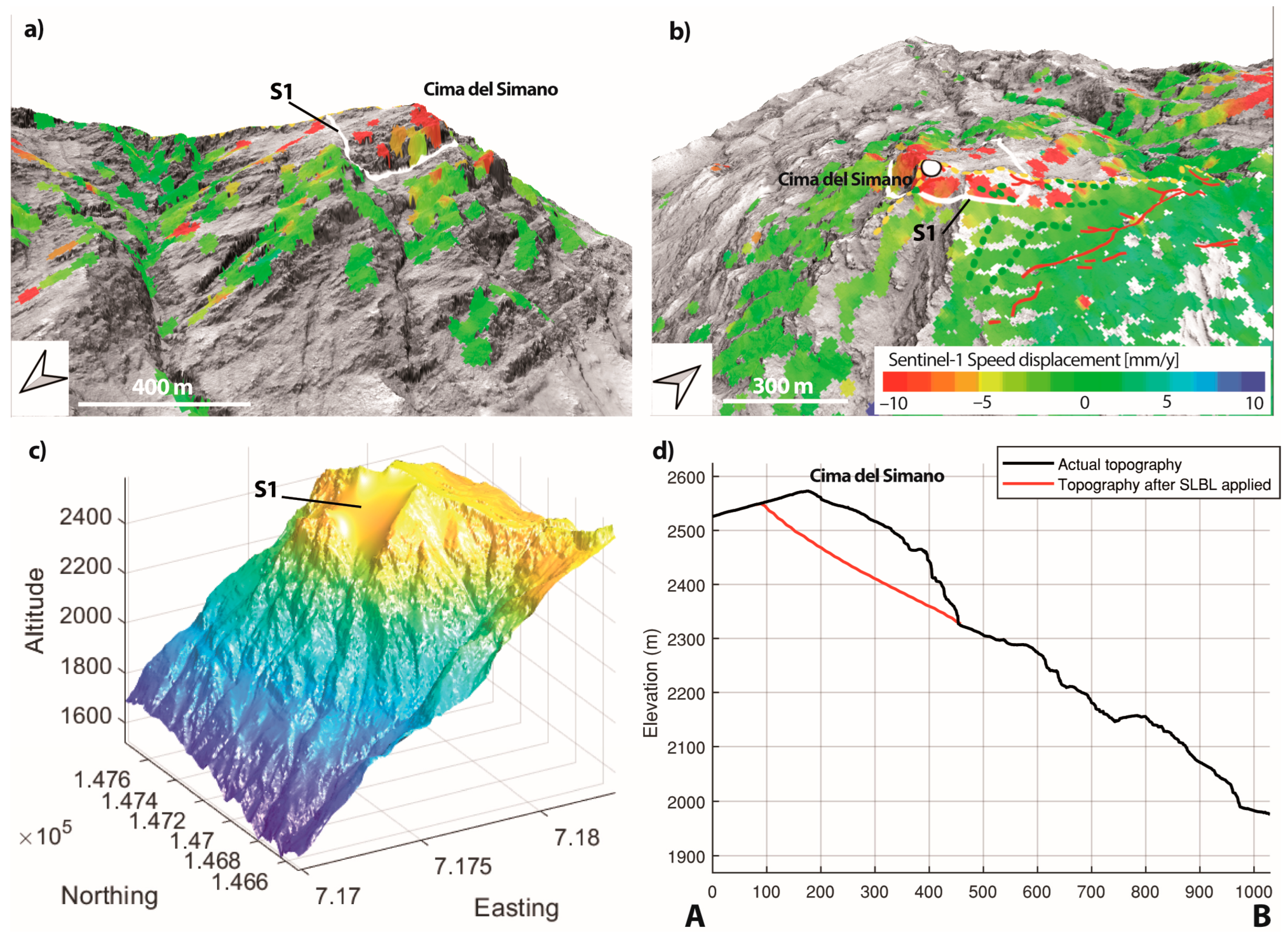
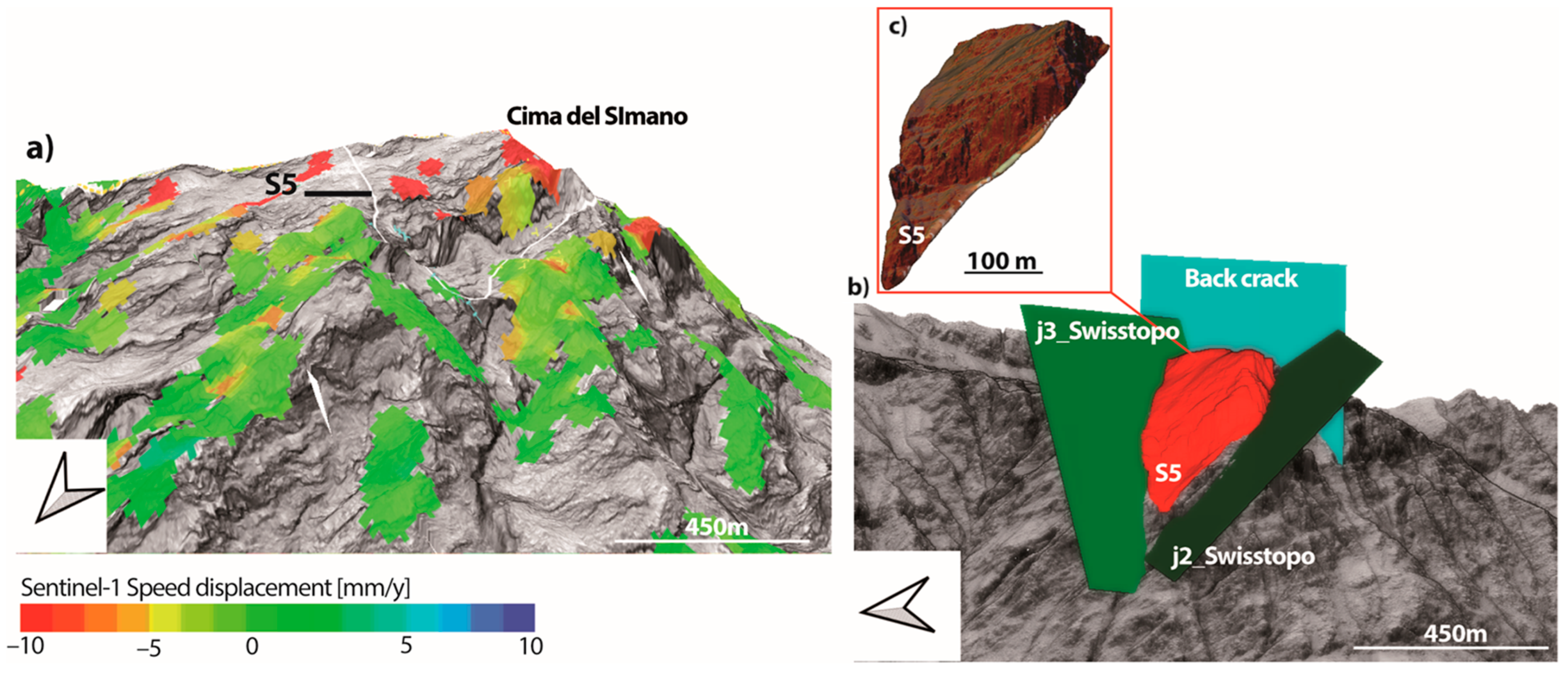
4. Results
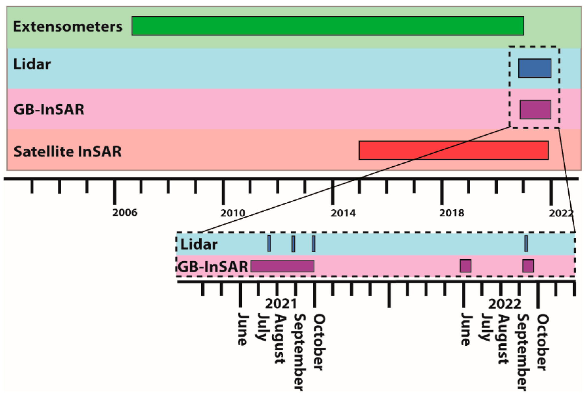
4.1. Monitoring Results
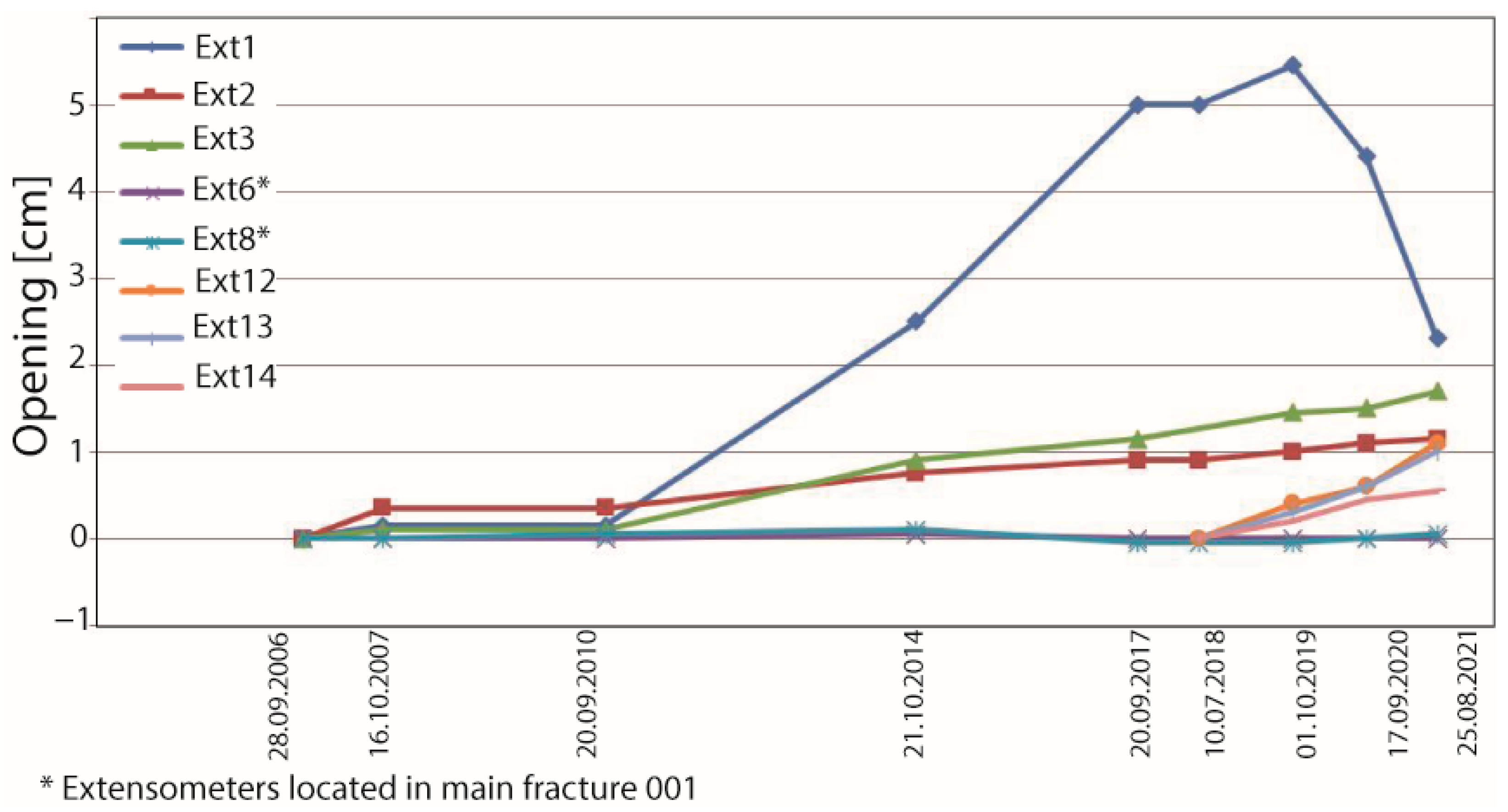
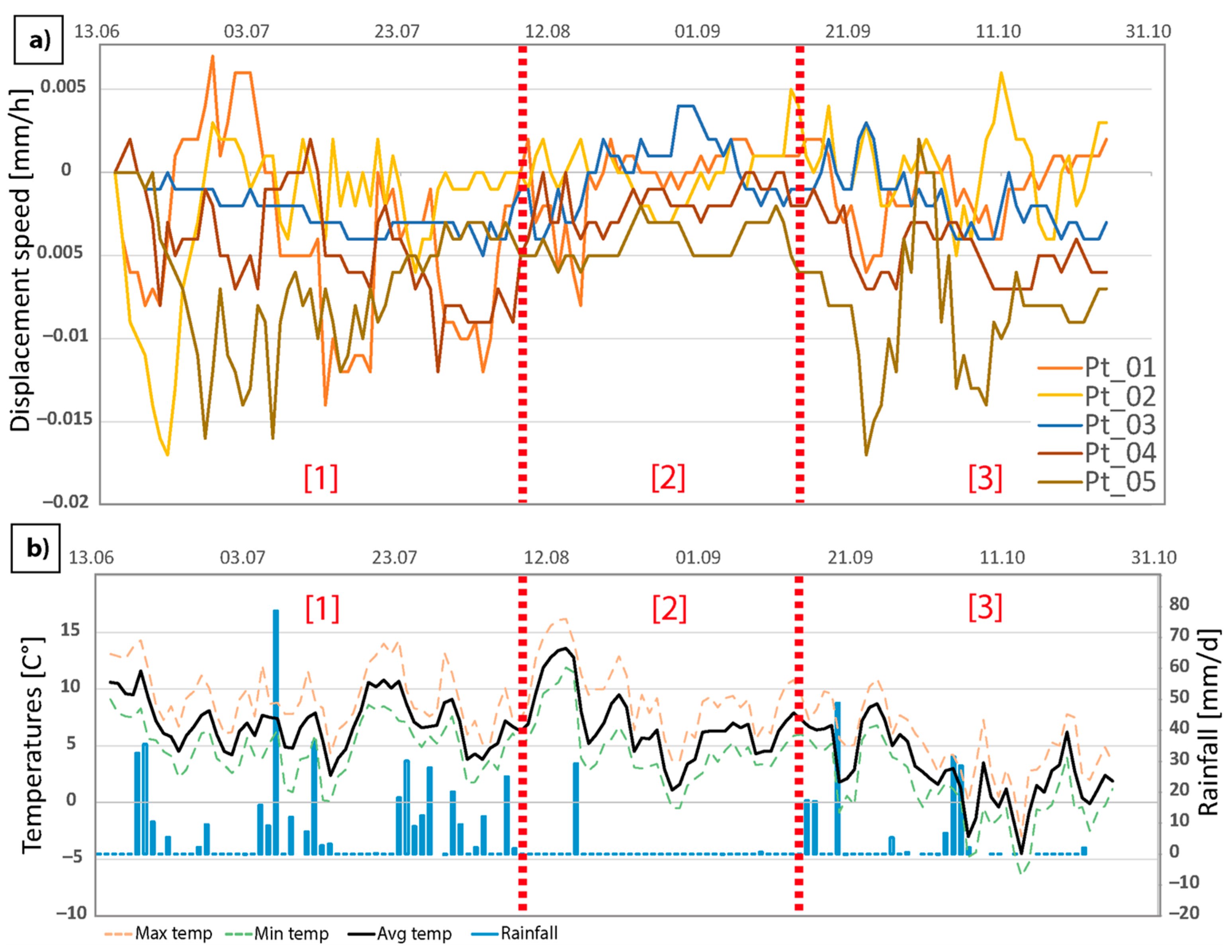
4.1.1. Extensometers Results
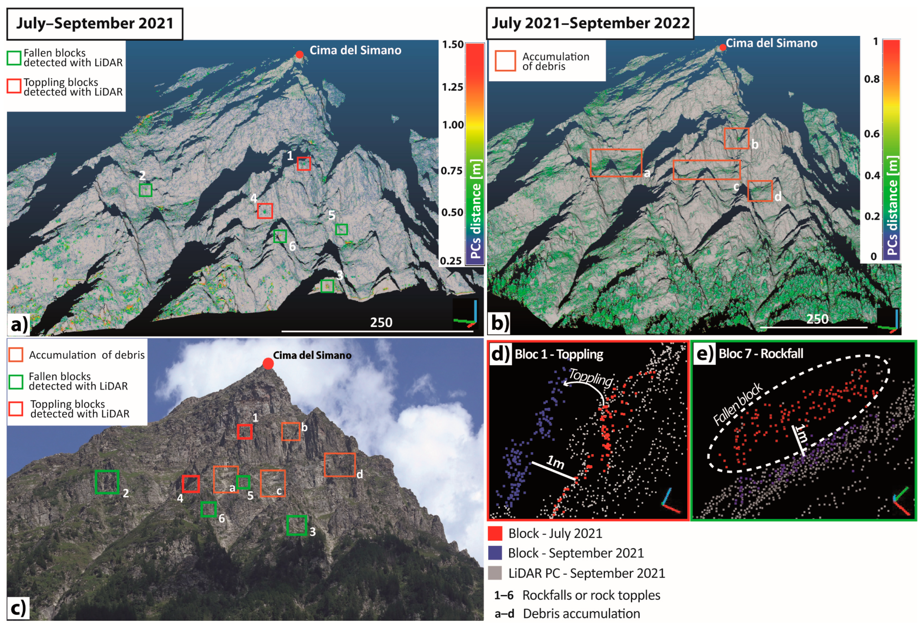
4.1.2. LiDAR Results
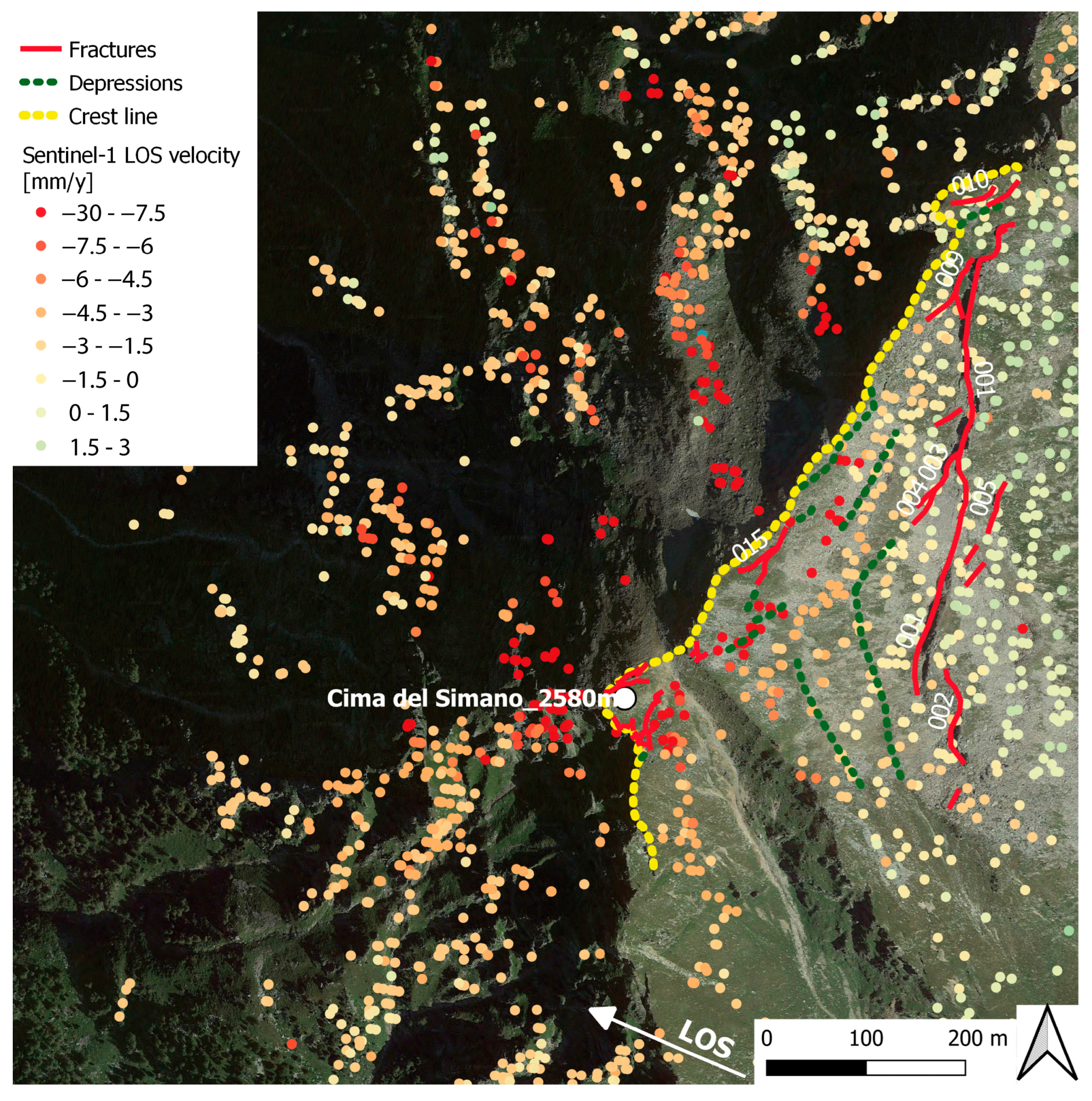
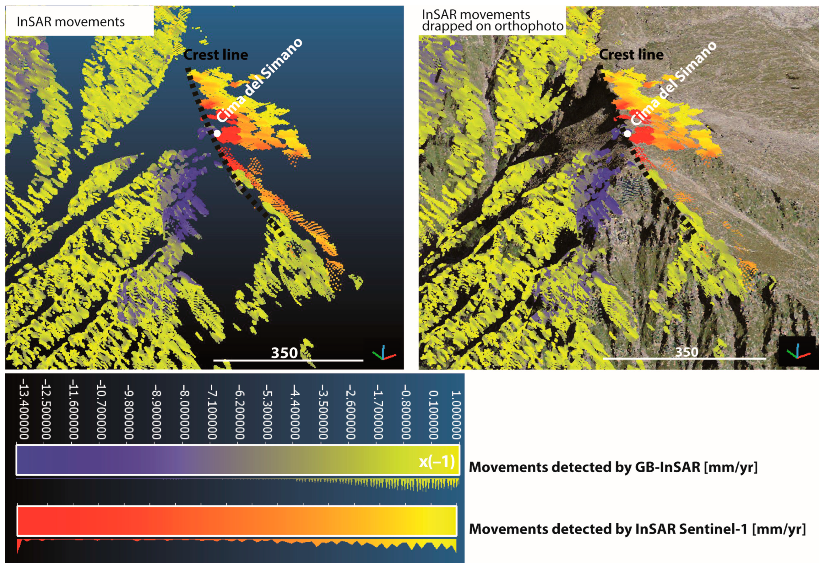
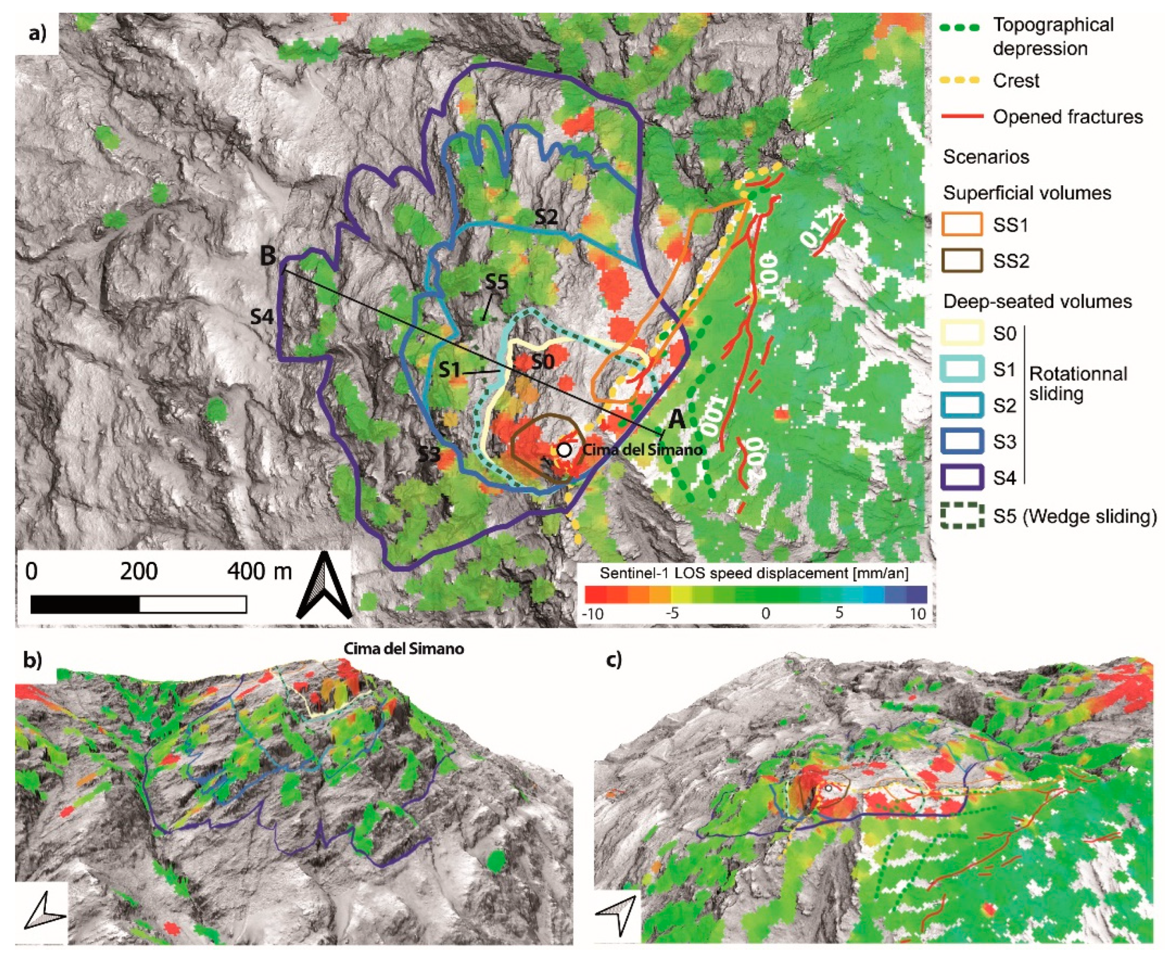
4.1.3. GB-InSAR Results and InSAR Interpretations
4.1.4. Weather Results
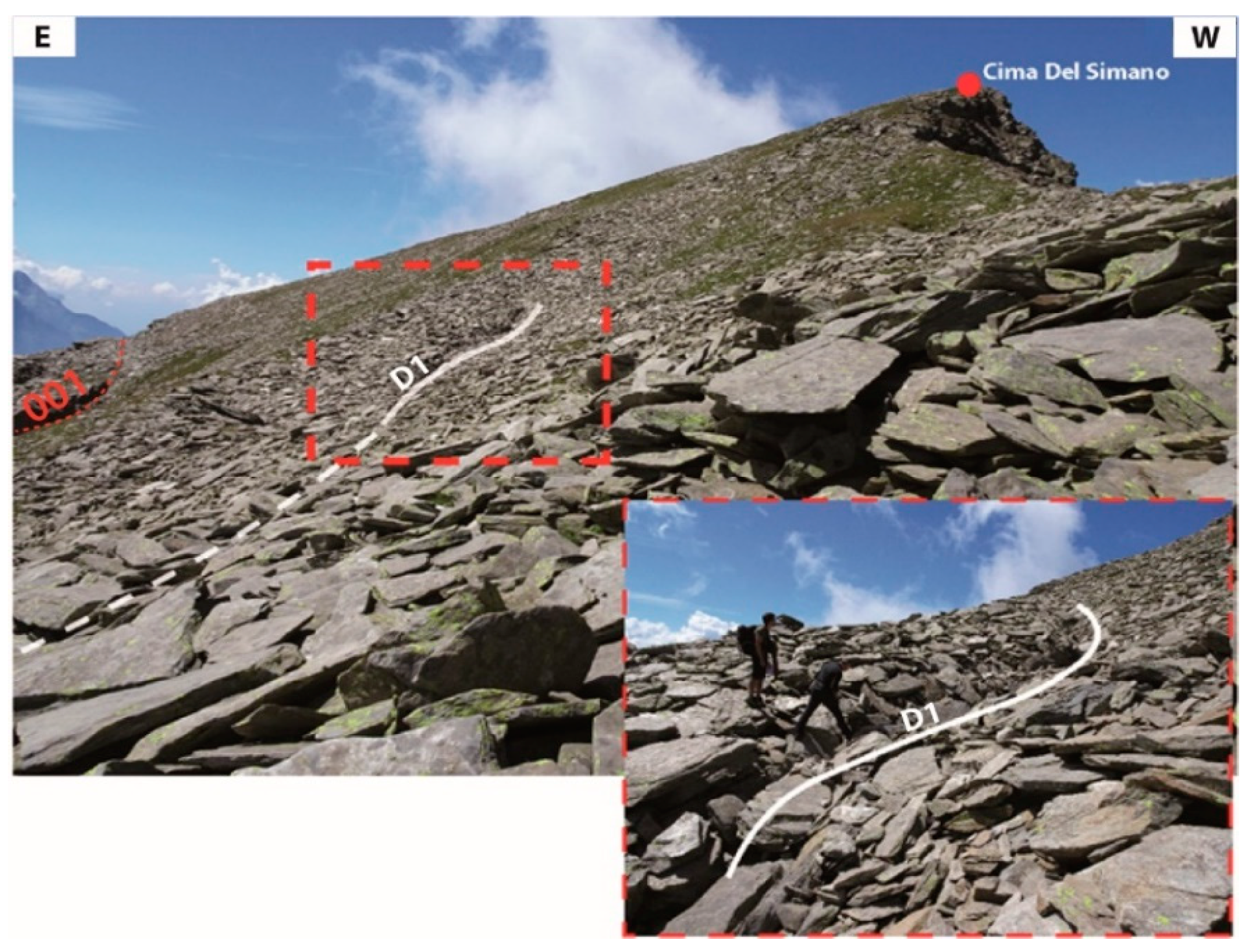
4.2. Structure Analysis
5. Discussion
5.1. Weather Impact
5.1.1. Temperatures Analysis Results
5.1.2. Rainfalls Analysis Results
5.2. Limitations of the Manual Extensometers
5.3. Scenarios for Rockfall and Rockslide Hazards

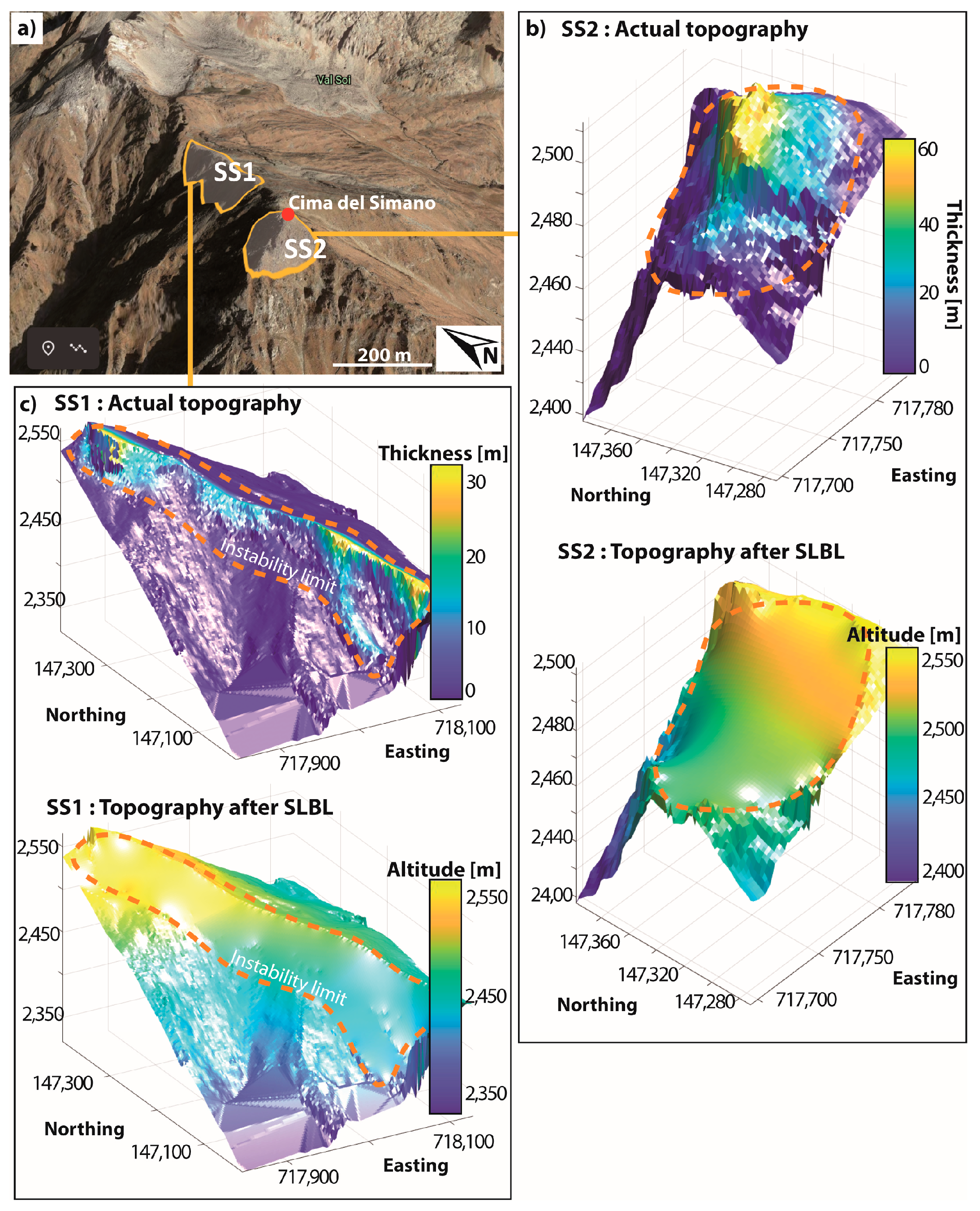
| Instability Failure Mode | Scenario | Length [m] | Surface [m2] | Volume [m3] | Mean Thickness [m] | Curvature Tolerance C | Arguments in Favor of the Scenario |
|---|---|---|---|---|---|---|---|
| Superficial movement, Sliding or toppling | SS1 1 | 50 | - | 230k | - | 0 | Fresh soil in some fractures Blocks toppling visible in the field Toppling blocks detected by LiDAR and InSAR |
| Superficial movement Sliding or toppling | SS2 1 | 70 | - | 251k | - | 0 | |
| Deep-seated rotational movement | S0 | 200 | 63,000 | 3.8M | 20 | 0.33 | Delimitated by the displacements detected by GB-InSAR only |
| Deep-seated rotational movement | S1 1 | 300 | 87,500 | 4.3M | 30 | 0.043 | Delimitated by the displacements detected by GB- and satellite InSAR |
| Deep-seated rotational movement | S2 | 400 | 178,000 | 16M | 70 | 0.039 | Encompasses the moving area detected by InSAR Follow the topography along the isoline at the altitude of 2200 m |
| Deep-seated rotational movement | S3 | 450 | 241,000 | 22M | 80 | 0.033 | Encompasses the moving area detected by InSAR Follow the topography along the isoline at the altitude of 2000 m |
| Deep-seated rotational movement | S4 | 600 | 451,000 | 51M | 110 | 0.024 | Encompasses the moving area detected by InSAR Follow the topography along the isoline at the altitude of 1900 m |
| Deep-seated sliding constrained by two plans | S5 1 | 320 | 76,200 | 7.7M | - | - | Delimitated by the displacements detected by GB- and satellite InSAR Constrained by two plans from j2 and j3 |


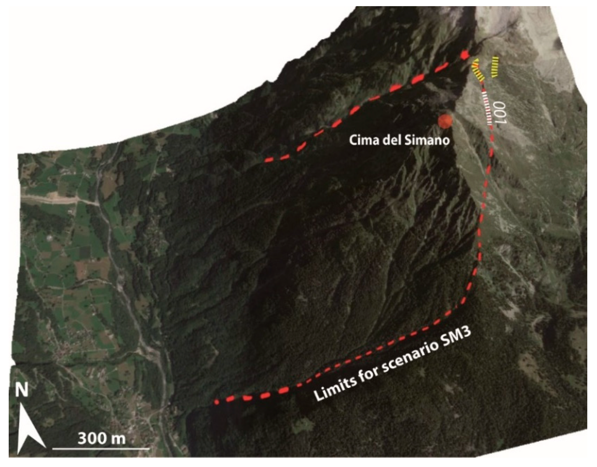
5.4. Scenario SM3: Case of the Main Open Fracture ‘001’
5.5. Susceptibility Assessment
6. Conclusions
Supplementary Materials
Author Contributions
Funding
Data Availability Statement
Acknowledgments
Conflicts of Interest
References
- Marcato, G.; Mantovani, M.; Pasuto, A.; Zabuski, L.; Borgatti, L. Monitoring, Numerical Modelling and Hazard Mitigation of the Moscardo Landslide (Eastern Italian Alps). Eng. Geol. 2012, 128, 95–107. [Google Scholar] [CrossRef]
- Crosta, G.B.; di Prisco, C.; Frattini, P.; Frigerio, G.; Castellanza, R.; Agliardi, F. Chasing a Complete Understanding of the Triggering Mechanisms of a Large Rapidly Evolving Rockslide. Landslides 2014, 11, 747–764. [Google Scholar] [CrossRef]
- Carlà, T.; Tofani, V.; Lombardi, L.; Raspini, F.; Bianchini, S.; Bertolo, D.; Thuegaz, P.; Casagli, N. Combination of GNSS, Satellite InSAR, and GBInSAR Remote Sensing Monitoring to Improve the Understanding of a Large Landslide in High Alpine Environment. Geomorphology 2019, 335, 62–75. [Google Scholar] [CrossRef]
- Pollet, N. Large High-Speed Gravity Rock Slope Movements: Contributions of Field Observations in Order to Understand Propagation and Deposition Processes. Application to Three Alpine Cases: La Madeleine (Savoie, France), Flims (Graubunden, Switzerland) and Köfels (Tyrol, Austria); Ecole des Ponts ParisTech: Paris, France, 2004. [Google Scholar]
- Stead, D.; Wolter, A. A Critical Review of Rock Slope Failure Mechanisms: The Importance of Structural Geology. J. Struct. Geol. 2015, 74, 1–23. [Google Scholar] [CrossRef]
- Sartori, M.; Baillifard, F.; Jaboyedoff, M.; Rouiller, J.-D. Kinematics of the 1991 Randa Rockslides (Valais, Switzerland). Nat. Hazards Earth Syst. Sci. 2003, 3, 423–433. [Google Scholar] [CrossRef]
- Oppikofer, T.; Jaboyedoff, M.; Pedrazzini, A.; Derron, M.; Blikra, L.H. Detailed DEM Analysis of a Rockslide Scar to Characterize the Basal Sliding Surface of Active Rockslides. J. Geophys. Res. 2011, 116, F2. [Google Scholar] [CrossRef]
- Pedrazzini, A.; Jaboyedoff, M.; Froese, C.R.; Langenberg, C.W.; Moreno, F. Structural Analysis of Turtle Mountain: Origin and Influence of Fractures in the Development of Rock Slope Failures. Geol. Soc. 2011, 351, 163–183. [Google Scholar] [CrossRef]
- Jomard, H. Analyse Multi-Échelles des Déformations Gravitaires du Massif de L’Argentera Mercantour; Université Nice Sophia Antipolis: Nice, France, 2006. [Google Scholar]
- El Bedoui, S.; Guglielmi, Y.; Lebourg, T.; Pérez, J.-L. Deep-Seated Failure Propagation in a Fractured Rock Slope over 10,000 Years: The La Clapière Slope, the South-Eastern French Alps. Geomorphology 2009, 105, 232–238. [Google Scholar] [CrossRef]
- Agliardi, F.; Crosta, G.B.; Zanchi, A.; Ravazzi, C. Onset and Timing of Deep-Seated Gravitational Slope Deformations in the Eastern Alps, Italy. Geomorphology 2009, 103, 113–129. [Google Scholar] [CrossRef]
- Pedrazzini, A.; Jaboyedoff, M.; Loye, A.; Derron, M.-H. From Deep Seated Slope Deformation to Rock Avalanche: Destabilization and Transportation Models of the Sierre Landslide (Switzerland). Tectonophysics 2013, 605, 149–168. [Google Scholar] [CrossRef]
- Pedrozzi, G. Triggering of Landslides in Canton Ticino (Switzerland) and Prediction by the Rainfall Intensity and Duration Method. Bull. Eng. Geol. Environ. 2004, 63, 281–291. [Google Scholar] [CrossRef]
- Seno, S.; Thüring, M. Large Landslides in Ticino, Southern Switzerland: Geometry and Kinematics. Eng. Geol. 2006, 83, 109–119. [Google Scholar] [CrossRef]
- Claude, A.; Ivy-Ochs, S.; Kober, F.; Antognini, M.; Salcher, B.; Kubik, P.W. The Chironico Landslide (Valle Leventina, Southern Swiss Alps): Age and Evolution. Swiss J. Geosci. 2014, 107, 273–291. [Google Scholar] [CrossRef]
- Liechti, K.; Matter, D.; Lustenberger, F.; Badoux, A. Wasser, Energie, Luft. 2022. Available online: https://www.researchgate.net/profile/Sandra-Melzner/publication/365651341_Impact_of_quality_of_input_data_on_3D_rockfall_modelling/links/637cfe6737878b3e87d155e3/Impact-of-quality-of-input-data-on-3D-rockfall-modelling.pdf#page=590 (accessed on 12 January 2023).
- Bonnard, C. Buzza di Biasca. Available online: https://hls-dhs-dss.ch/fr/articles/028662/2004-11-04/ (accessed on 12 January 2023).
- De Pedrini, A.; Ambrosi, C.; Scapozza, C. The 1513 Monte Crenone Rock Avalanche: Numerical Model and Geomorphological Analysis. Geogr. Helv. 2022, 77, 21–37. [Google Scholar] [CrossRef]
- Rabatel, A.; Deline, P.; Jaillet, S.; Ravanel, L. Rock Falls in High-Alpine Rock Walls Quantified by Terrestrial Lidar Measurements: A Case Study in the Mont Blanc Area. Geophys. Res. Lett. 2008, 35, 10. [Google Scholar] [CrossRef]
- Carrea, D.; Abellan, A.; Derron, M.-H.; Jaboyedoff, M. Automatic Rockfalls Volume Estimation Based on Terrestrial Laser Scanning Data. In Engineering Geology for Society and Territory; Lollino, G., Giordan, D., Crosta, G.B., Corominas, J., Azzam, R., Wasowski, J., Sciarra, N., Eds.; Springer International Publishing: Cham, Switzerland, 2015; Volume 2, pp. 425–428. ISBN 978-3-319-09056-6. [Google Scholar]
- Abellan, A.; Derron, M.-H.; Jaboyedoff, M. “Use of 3D Point Clouds in Geohazards” Special Issue: Current Challenges and Future Trends. Remote Sens. 2016, 8, 130. [Google Scholar] [CrossRef]
- Slob, S.; Hack, R.; Turner, A.K. An Approach to Automate Discontinuity Measurements of Rock Faces Using Laser Scanning Techniques. In Proceedings of the ISRM International Symposium, EUROCK 2002, Madere, Portugal, 25–27 November 2002; pp. 87–94. [Google Scholar]
- Slob, S.; Hack, R. 3D Terrestrial Laser Scanning as a New Field Measurement and Monitoring Technique. In Engineering Geology for Infrastructure Planning in Europe; Hack, R., Azzam, R., Charlier, R., Eds.; Lecture Notes in Earth Sciences; Springer: Berlin/Heidelberg, Germany, 2004; Volume 104, pp. 179–189. ISBN 978-3-540-21075-7. [Google Scholar]
- Malet, J.-P.; Maquaire, O.; Calais, E. The Use of Global Positioning System Techniques for the Continuous Monitoring of Landslides: Application to the Super-Sauze Earthflow (Alpes-de-Haute-Provence, France). Geomorphology 2002, 43, 33–54. [Google Scholar] [CrossRef]
- Eyo, E.E.; Musa, T.A.; Omar, K.M.; Idris, K.M.; Bayrak, T.; Onuigbo, I.C.; Opaluwa, Y.D. Application of Low-Cost GPS Tools and Techniques for Landslide Monitoring: A Review. J. Teknol. 2014, 71, 71–78. [Google Scholar] [CrossRef]
- Tarchi, D.; Casagli, N.; Fanti, R.; Leva, D.D.; Luzi, G.; Pasuto, A.; Pieraccini, M.; Silvano, S. Landslide Monitoring by Using Ground-Based SAR Interferometry: An Example of Application to the Tessina Landslide in Italy. Eng. Geol. 2003, 68, 15–30. [Google Scholar] [CrossRef]
- Bardi, F.; Frodella, W.; Ciampalini, A.; Bianchini, S.; Del Ventisette, C.; Gigli, G.; Fanti, R.; Moretti, S.; Basile, G.; Casagli, N. Integration between Ground Based and Satellite SAR Data in Landslide Mapping: The San Fratello Case Study. Geomorphology 2014, 223, 45–60. [Google Scholar] [CrossRef]
- Lazecký, M.; Çomut, F.C.; Hlaváčová, I.; Gürboğa, Ş. Practical Application of Satellite-Based SAR Interferometry for the Detection of Landslide Activity. Procedia Earth Planet. Sci. 2015, 15, 613–618. [Google Scholar] [CrossRef]
- Wood, H.M. Toward an Integrated Space Strategy for Disaster Management. In Early Warning Systems for Natural Disaster Reduction; Zschau, J., Küppers, A., Eds.; Springer: Berlin/Heidelberg, Germany, 2003; pp. 737–739. ISBN 978-3-642-63234-1. [Google Scholar]
- Huggel, C.; Frey, H.; Klimes, J.; Strozzi, T.; Caduff, R.; Cochachin, A. Contribution of Earth Observation to Landslide Early Warning; ESA Alcantara No. 5: InSAR and Landslides in Peru. 2017. Available online: http://www.geo.uzh.ch/~chuggel/files_download/alcantara/eo_ews_white_paper_esa_alcantara_2017.pdf (accessed on 15 November 2023).
- Michelini, A.; Viviani, F.; Bianchetti, M.; Coli, N.; Leoni, L.; Stopka, C. A New Radar-Based System for Detecting and Tracking Rockfall in Open Pit Mines. In Proceedings of the 2020 International Symposium on Slope Stability in Open Pit Mining and Civil Engineering, Perth, WA, Australia, 12–14 May 2020; pp. 1183–1192. [Google Scholar]
- Carlà, T.; Gigli, G.; Lombardi, L.; Nocentini, M.; Meier, L.; Schmid, L.; Wahlen, S.; Casagli, N. Real-Time Detection and Management of Rockfall Hazards by Ground-Based Doppler Radar. Landslides 2023, 19, 1–9. [Google Scholar] [CrossRef]
- Schneider, M.; Oestreicher, N.; Loew, S. Rockfall Monitoring with a Doppler Radar on an Active Rock Slide Complex in Brienz/Brinzauls (Switzerland). Nat. Hazards Earth Syst. Sci. 2023, 23, 3337–3354. [Google Scholar] [CrossRef]
- Teza, G.; Pesci, A.; Genevois, R.; Galgaro, A. Characterization of Landslide Ground Surface Kinematics from Terrestrial Laser Scanning and Strain Field Computation. Geomorphology 2008, 97, 424–437. [Google Scholar] [CrossRef]
- Yin, Y.; Zheng, W.; Liu, Y.; Zhang, J.; Li, X. Integration of GPS with InSAR to Monitoring of the Jiaju Landslide in Sichuan, China. Landslides 2010, 7, 359–365. [Google Scholar] [CrossRef]
- Jaboyedoff, M.; Oppikofer, T.; Abellán, A.; Derron, M.-H.; Loye, A.; Metzger, R.; Pedrazzini, A. Use of LIDAR in Landslide Investigations: A Review. Nat. Hazards 2012, 61, 5–28. [Google Scholar] [CrossRef]
- Scapozza, C.; Tognacca, C.; Ambrosi, C. 20 maggio 1515: La “Buzza” che impressionò l’Europa. Boll. Soc. Ticin. Sci. Nat. 2015, 103, 79–88. [Google Scholar]
- Mey, J.; Scherler, D.; Wickert, A.D.; Egholm, D.L.; Tesauro, M.; Schildgen, T.F.; Strecker, M.R. Glacial Isostatic Uplift of the European Alps. Nat. Commun. 2016, 7, 13382. [Google Scholar] [CrossRef] [PubMed]
- Ambrosi, C.; Castelletti, C.; Czerski, D.; Scapozza, C.; Schenker, F.L. The New Landslide and Rock Glacier Inventory Map of Canton Ticino. In Proceedings of the 20th EGU General Assembly Conference, Vienna, Austria, 4–13 April 2018; Volume 20, p. EGU2018–2358. [Google Scholar]
- Rütti, R.; Maxelon, M.; Mancktelow, N.S. Structure and Kinematics of the Northern Simano Nappe, Central Alps, Switzerland. Eclogae Geol. Helv. 2005, 98, 63–81. [Google Scholar] [CrossRef]
- Cavargna-Sani, M. (in Prep.): Foglio 1253 Olivone. Atlante Geologico Della Svizzera 1: 25,000; Swisstopo: Wabern, Switzerland, 2023. [Google Scholar]
- Leachtenauer, J.C.; Driggers, R.G. Surveillance and Reconnaissance Imaging Systems. In Surveillance and Reconnaissance Imaging Systems: Modeling and Performance Prediction; Artech House: Norwood, MA, USA, 2001; Chapter 2; pp. 30–31. ISBN 978-1-58053-132-0. [Google Scholar]
- Sturzenegger, M.; Yan, M.; Stead, D.; Elmo, D. Application and Limitations of Ground-Based Laser Scanning in Rock Slope Characterization. In Rock Mechanics: Meeting Society’s Challenges and Demands; Eberhardt, E., Stead, D., Morrison, T., Eds.; Taylor & Francis: Abingdon, UK, 2007; pp. 29–36. ISBN 978-0-415-44401-9. [Google Scholar]
- Rodeon-Pixplorer-2. Available online: https://dr-clauss.de/rodeon-pixplorer-2/ (accessed on 22 May 2023).
- Ferretti, A.; Monti-Guarnieri, A.; Prati, C.; Rocca, F.; Massonnet, D. SAR Images of the Earth’s Surface. In InSAR Principles: Guidelines for SAR Interferometry Processing and Interpretation; ESA Publications: The Hague, The Netherlands, 2007; pp. 11–38. ISBN 92-9092-233-8. [Google Scholar]
- Massonnet, D.; Briole, P.; Arnaud, A. Deflation of Mount Etna Monitored by Spaceborne Radar Interferometry. Nature 1995, 375, 567–570. [Google Scholar] [CrossRef]
- Fruneau, B.; Adache, J.; Delacourt, C. Observation and Modelling of the Saint-Ktienne-de-Tin&e Landslide Using SAR Interferometry. Techtonophysics 1996, 265, 181–190. [Google Scholar]
- Colesanti, C.; Ferretti, A.; Prati, C.; Rocca, F. Monitoring Landslides and Tectonic Motions with the Permanent Scatterers Technique. Eng. Geol. 2003, 68, 3–14. [Google Scholar] [CrossRef]
- Squarzoni, C.; Delacourt, C.; Allemand, P. Nine Years of Spatial and Temporal Evolution of the La Valette Landslide Observed by SAR Interferometry. Eng. Geol. 2003, 68, 53–66. [Google Scholar] [CrossRef]
- Rouyet, L.; Kristensen, L.; Derron, M.-H.; Michoud, C.; Blikra, L.H.; Jaboyedoff, M.; Lauknes, T.R. Evidence of Rock Slope Breathing Using Ground-Based InSAR. Geomorphology 2017, 289, 152–169. [Google Scholar] [CrossRef]
- Strozzi, T.; Antonova, S.; Günther, F.; Mätzler, E.; Vieira, G.; Wegmüller, U.; Westermann, S.; Bartsch, A. Sentinel-1 SAR Interferometry for Surface Deformation Monitoring in Low-Land Permafrost Areas. Remote Sens. 2018, 10, 1360. [Google Scholar] [CrossRef]
- Wegnüller, U.; Werner, C.; Strozzi, T.; Wiesmann, A.; Frey, O.; Santoro, M. Sentinel-1 Support in the GAMMA Software. Procedia Comput. Sci. 2016, 100, 1305–1312. [Google Scholar] [CrossRef]
- Mahafza, B.R. Radar Systems Analysis and Design Using Matlab; Chapman & Hall/CRC: Boca Raton, FL, USA, 2000; ISBN 978-1-58488-182-7. [Google Scholar]
- Noferini, L.; Pieraccini, M.; Mecatti, D.; Luzi, G.; Atzeni, C.; Tamburini, A.; Broccolato, M. Permanent Scatterers Analysis for Atmospheric Correction in Ground-Based SAR Interferometry. IEEE Trans. Geosci. Remote Sens. 2005, 43, 1459–1471. [Google Scholar] [CrossRef]
- Pipia, L.; Fabregas, X.; Aguasca, A.; Lopez-Martinez, C. Atmospheric Artifact Compensation in Ground-Based DInSAR Applications. IEEE Geosci. Remote Sens. Lett. 2008, 5, 88–92. [Google Scholar] [CrossRef]
- Hoek, E.; Bray, J.W. Rock Slope Engineering, 3rd ed.; The Institution of Mining and Metallurgy: London, UK, 1981; pp. 341–351. [Google Scholar]
- Wyllie, D.-C. Foundations on Rock, 2nd ed.; Taylor & Francis: London, UK, 1999; ISBN 978-0-367-86575-7. [Google Scholar]
- Neuendorf, K.K.E.; Mehl, J.P.; Jackson, J.A. Glossary of Geology, 5th ed.; Springer Science & Business Media: New York, NY, USA, 2005. [Google Scholar]
- Fossen, H. Structural Geology; Cambridge University Press: New York, NY, USA, 2010. [Google Scholar]
- Humair, F.; Pedrazzini, A.; Epard, J.-L.; Froese, C.R.; Jaboyedoff, M. Structural Characterization of Turtle Mountain Anticline (Alberta, Canada) and Impact on Rock Slope Failure. Tectonophysics 2013, 605, 133–148. [Google Scholar] [CrossRef]
- Markland, J.T. A Useful Technique for Estimating the Stability of Rock Slopes When the Rigid Wedge Sliding Type of Failure Is Expected; Imperial College of Science and Technology: London, UK, 1972. [Google Scholar]
- Taboni, B.; Tagliaferri, I.D.; Umili, G. A Tool for Performing Automatic Kinematic Analysis on Rock Outcrops. Geosciences 2022, 12, 435. [Google Scholar] [CrossRef]
- Carrell, J. Tools and Techniques for 3D Geologic Mapping in ArcScene: Boreholes, Cross Sections, and Block Diagrams. US Geol. Surv. Open-File Rep. 2014, 2014, 1167. [Google Scholar]
- Jaboyedoff, M.; Baillifard, F.; Couture, R.; Locat, J.; Locat, P. Toward Preliminary Hazard Assessment Using DEM Topographic Analysis and Simple Mechanical Modeling by Means of Sloping Local Base Level; CRC Press: Boca Raton, FL, USA, 2004; ISBN 978-0-415-35665-7. [Google Scholar]
- Jaboyedoff, M.; Carrea, D.; Derron, M.-H.; Oppikofer, T.; Penna, I.M.; Rudaz, B. A Review of Methods Used to Estimate Initial Landslide Failure Surface Depths and Volumes. Eng. Geol. 2020, 267, 105478. [Google Scholar] [CrossRef]
- Agliardi, F.; Crosta, G.; Zanchi, A. Structural Constraints on Deep-Seated Slope Deformation Kinematics. Eng. Geol. 2001, 59, 83–102. [Google Scholar] [CrossRef]
- Delgado, J.; Vicente, F.; García-Tortosa, F.; Alfaro, P.; Estévez, A.; Lopez-Sanchez, J.M.; Tomás, R.; Mallorquí, J.J. A Deep Seated Compound Rotational Rock Slide and Rock Spread in SE Spain: Structural Control and DInSAR Monitoring. Geomorphology 2011, 129, 252–262. [Google Scholar] [CrossRef]
- Bracewell, R. Pentagram Notation for Cross Correlation. In The Fourier Transform and Its Applications; McGraw-Hill: New York, USA, 1965; pp. 46–243. [Google Scholar]
- Carrión-García, A.; Jabaloyes, J.; Grisales, A. The Growth of COVID-19 in Spain. A View Based on Time-Series Forecasting Methods. In Data Science for COVID-19 Computational Perspectives; Academic Press: Cambridge, MA, USA, 2021; Volume 1, pp. 643–660. ISBN 978-0-12-824536-1. [Google Scholar]
- OFEN Map of Potential Permafrost Distribution. 2005. Available online: https://map.geo.admin.ch/ (accessed on 11 September 2023).
- Guerin, A.; Jaboyedoff, M.; Collins, B.D.; Stock, G.M.; Derron, M.-H.; Abellán, A.; Matasci, B. Remote Thermal Detection of Exfoliation Sheet Deformation. Landslides 2021, 18, 865–879. [Google Scholar] [CrossRef] [PubMed]
- Girardeau-Montaut, D. CloudCompare 2015. Available online: https://www.cloudcompare.org/doc/wiki/index.php/Main_Page (accessed on 16 January 2023).
- Jaboyedoff, M.; Blikra, L.; Crosta, G.B.; Froese, C.; Hermanns, R.; Oppikofer, T.; Böhme, M.; Stead, D. Fast Assessment of Susceptibility of Massive Rock Instabilities. In Landslides and Engineered Slopes. Protecting Society through Improved Understanding; CRC Press: Banff, AL, Canada, 2012; pp. 459–465. [Google Scholar]
- Huisman, M.; Nieuwenhuis, J.D.; Hack, H.R.G.K. Numerical Modelling of Combined Erosion and Weathering of Slopes in Weak Rock: Combined erosion and weathering of slopes in weak rock. Earth Surf. Process. Landf. 2011, 36, 1705–1714. [Google Scholar] [CrossRef]
- Sengani, F.; Mulenga, F. Application of Limit Equilibrium Analysis and Numerical Modeling in a Case of Slope Instability. Sustainability 2020, 12, 8870. [Google Scholar] [CrossRef]
- Fu, Y.; Liu, Z.; Zeng, L.; Gao, Q.; Luo, J.; Xiao, X. Numerical Analysis Method that Considers Weathering and Water-Softening Effects for the Slope Stability of Carbonaceous Mudstone. IJERPH 2022, 19, 14308. [Google Scholar] [CrossRef]


| Remote Sensing Technique | Acquisition Frequency | Spatial Resolution | Minimum Measurable Displacement | Range Acquisition Distance | Device Used | Movement Types Recorded |
|---|---|---|---|---|---|---|
| Extensometers | 1/year | One-off measure | 1 mm | In fracture Daily monitoring from office | Measuring tape | Slow movements of big volume and extent |
| LiDAR | 1/month during 3 months in 2021 | 30 cm 1 | 30 cm | From valley 3.5 km | Riegl VZ6000 | Rockfall and toppling activity |
| GB-InSAR | 2/year in 2022, 3 consecutive months in 2021 | 3 m | ~1 mm | From valley 3.5 km Daily monitoring from office | Ellegis LisaLab with a 3 m synthetic antenna aperture | Slow movements of big volume and extent Superficial topplings |
| Satellite InSAR | 2 weeks | 5 m | ~1–2 mm | From orbit 693 km altitude | Satellite Sentinel-1 | Slow movements of big volume and extent |
| (a) Measurements in the field | |||
| Dip/Dip Direction | Quantity | ||
| j1 | 73°/178° | 25 | |
| j2 | 89°/294° | 18 | |
| s1 | 19°/018° | 50 | |
| not classified | - | 38 | |
| (b) From PCs analysis with Coltop | |||
| Dip/Dip Direction | |||
| LiDAR | Drone | Swisstopo DEM | |
| j1 | 72°/180° | 70°/190° | 45°/173° 2 |
| j2 | 65°/285° | 56°/283° | 46°/268° 2 |
| j3 | - | - | 47°/349° 2 |
| s1 | - | 26°/080° | - |
| Intersection j2/j3 1 | 42°/197° | 46°/211° | 39°/234° |
| (c) From the geological map and orthophoto | |||
| Dip/Dip Direction | Orientation | ||
| s1 | 20°/035° | - | |
| fault 1 | 76°/246° | - | |
| fault 2 | 59°/181° | - | |
| Lineament 1 | - | 85° | |
| Lineament 2 | - | 330° | |
| Scenario | Length [m] | Displacement Speed [mm/y] | Deformation Rate [%/y] | Deformation State (After [73]) | Susceptibility |
|---|---|---|---|---|---|
| SS1 | 50 | 9 | 0.018 | 2-2 | High |
| SS2 | 70 | 11 | 0.016 | 2-2 | High |
| S0 | 200 | 7 | 0.0035 | 2-1 | Moderate to high |
| S1 | 300 | 7 | 0.0023 | 2-1 | Moderate to high |
| S2 | 400 | 7 | 0.0018 | 2-1 | Low to moderate |
| S3 | 450 | 7 | 0.0016 | 2-1 | Low to moderate |
| S4 | 600 | 7 | 0.0012 | 2-1 | Low to moderate |
| S5 | 200 | 7 | 0.0028 | 2-1 | Moderate to high |
Disclaimer/Publisher’s Note: The statements, opinions and data contained in all publications are solely those of the individual author(s) and contributor(s) and not of MDPI and/or the editor(s). MDPI and/or the editor(s) disclaim responsibility for any injury to people or property resulting from any ideas, methods, instructions or products referred to in the content. |
© 2023 by the authors. Licensee MDPI, Basel, Switzerland. This article is an open access article distributed under the terms and conditions of the Creative Commons Attribution (CC BY) license (https://creativecommons.org/licenses/by/4.0/).
Share and Cite
Wolff, C.; Jaboyedoff, M.; Fei, L.; Pedrazzini, A.; Derron, M.-H.; Rivolta, C.; Merrien-Soukatchoff, V. Assessing the Hazard of Deep-Seated Rock Slope Instability through the Description of Potential Failure Scenarios, Cross-Validated Using Several Remote Sensing and Monitoring Techniques. Remote Sens. 2023, 15, 5396. https://doi.org/10.3390/rs15225396
Wolff C, Jaboyedoff M, Fei L, Pedrazzini A, Derron M-H, Rivolta C, Merrien-Soukatchoff V. Assessing the Hazard of Deep-Seated Rock Slope Instability through the Description of Potential Failure Scenarios, Cross-Validated Using Several Remote Sensing and Monitoring Techniques. Remote Sensing. 2023; 15(22):5396. https://doi.org/10.3390/rs15225396
Chicago/Turabian StyleWolff, Charlotte, Michel Jaboyedoff, Li Fei, Andrea Pedrazzini, Marc-Henri Derron, Carlo Rivolta, and Véronique Merrien-Soukatchoff. 2023. "Assessing the Hazard of Deep-Seated Rock Slope Instability through the Description of Potential Failure Scenarios, Cross-Validated Using Several Remote Sensing and Monitoring Techniques" Remote Sensing 15, no. 22: 5396. https://doi.org/10.3390/rs15225396