Article

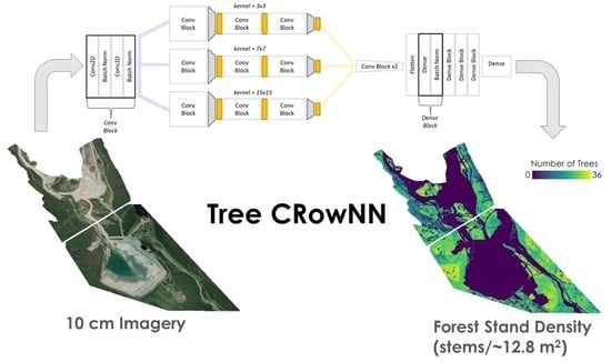
Tree-CRowNN: A Network for Estimating Forest Stand Density from VHR Aerial Imagery

1
Natural Resources Canada, Canada Centre for Mapping and Earth Observation, Ottawa, ON K1A 0E8, Canada
2
Department of Geography and Environmental Studies, Carleton University, Ottawa, ON K1S 5B6, Canada
*
Author to whom correspondence should be addressed.
Remote Sens. 2023, 15(22), 5307; https://doi.org/10.3390/rs15225307
Submission received: 29 September 2023 / Revised: 3 November 2023 / Accepted: 8 November 2023 / Published: 9 November 2023

Abstract

:
Estimating the number of trees within a forest stand, i.e., the forest stand density (FSD), is challenging at large scales. Recently, researchers have turned to a combination of remote sensing and machine learning techniques to derive these estimates. However, in most cases, the developed models rely heavily upon additional data such as LiDAR-based elevations or multispectral information and are mostly applied to managed environments rather than natural/mixed forests. Furthermore, they often require the time-consuming manual digitization or masking of target features, or an annotation using a bounding box rather than a simple point annotation. Here, we introduce the Tree Convolutional Row Neural Network (Tree-CRowNN), an alternative model for tree counting inspired by Multiple-Column Neural Network architecture to estimate the FSD over 12.8 m × 12.8 m plots from high-resolution RGB aerial imagery. Our model predicts the FSD with very high accuracy (MAE: ±2.1 stems/12.8 m2, RMSE: 3.0) over a range of forest conditions and shows promise in linking to Sentinel-2 imagery for broad-scale mapping (R2: 0.43, RMSE: 3.9 stems/12.8 m2). We believe that the satellite imagery linkage will be strengthened with future efforts, and transfer learning will enable the Tree-CRowNN model to predict the FSD accurately in other ecozones.

Graphical Abstract

1. Introduction

The count of trees within a forest stand, also known as the forest stand density (FSD), is an important metric for ecologists and natural resource managers [1]. This information can be used to interpret and rank the severity of disturbances such as pest infestations, forest fires, and flood events, by describing the damage in absolute terms (e.g., the number of trees lost) [2]. In healthy forests, the FSD can be used to estimate the stand age, yield projections, above-ground biomass, growth sustainability/growing stock, water balance, and arboreal carbon stocks [1,3,4,5]. The presence and density of woody stems in flood plains and other areas where flooding may occur has an important yet poorly understood influence on water flow and flood risk [6]. There is also a strong linkage between forest density and fire occurrence and severity [7]. Stephens et al. related tree densities and basal area to the relativized delta normalized burn ratio (RdNBR) for the 2020 Creek Fire in Southern Sierra Nevada, USA [7]. The authors of this study noted that dead and live tree densities were the strongest predictors of fire severity, with high densities being strongly and positively related to high-severity burns [7]. Under a changing climate, Canada is expected to see an increase in the occurrence and severity of catastrophic floods and fire events [8]. Therefore, high-quality FSD maps are crucial for supporting activities such as natural hazard risk modelling and monitoring.
In Canada, tree counts are mainly collected with ground surveys over 50 m2–400 m2 forest plots [9]. However, conducting field surveys is expensive, time-consuming, and spatially limited. Researchers have turned to remote sensing and machine learning techniques to extract this valuable information over large areas. Satellites provide the best opportunity for large-scale mapping, but deriving accurate tree counts from moderate-resolution satellite imagery proves to be challenging [10]. At this level, forest conditions are often described using spectral indices such as Forest Density Index (FDI), Scale Shadow Index (SSI), and Normalized Difference Vegetation Index (NDVI) [11]. While these indices provide general information about vegetation health status and forest composition, they do not directly relate to the number of trees that exist within forest stands. This issue may be addressed by adopting integrated multi-scale workflows using convolutional neural networks (CNNs) [12,13]. Advancements in deep learning for object detection and increased availability of high-quality high-resolution imagery have caused an expansion in studies focused on detect and localize (D&L) methods. Models for D&L using CNNs have been developed for a variety of tasks, such as detecting lake debris, automatic modulation classification, people, lake boundaries, and chimneys [14,15,16,17,18]. These models can be used to track the position of objects in imagery for locational change detection over time.
Estimating tree counts from high-resolution aerial imagery is an expanding area of D&L research. In most examples of tree counting applications, researchers rely heavily upon information beyond RGB spectral bands, such as photogrammetric or LiDAR-derived elevation datasets and/or multi-spectral datasets, and often test their methods on managed environments such as plantations where vegetation grows in regular patterns [1,6,13,19,20,21,22,23,24]. There are a few examples of tree counts being estimated over a range of forest conditions, including natural conditions, from high-resolution RGB aerial imagery alone. Two primary approaches for the task of automated tree counting have emerged in the literature: D&L methods where some form of image segmentation or masking is required, and density mapping methods (DM) [1,2,25,26].
Detect and localize workflows developed for forestry applications usually require the manual delineation of individual tree crowns or at least the estimation of the location of individual trees with minimum bounding boxes, to generate accurate training datasets [1,2]. Various deep learning models can then use these data to predict tree location and counts (e.g., Mask R-CNN, U-Net, and YOLO) [1,26]. It has been noted that D&L workflows perform well when target features are sparsely distributed but can encounter challenges when applied to densely clustered conditions [1,27]. Furthermore, preparing training data is somewhat time-consuming as the manual delineation or annotation of bounding boxes requires considerable effort [28].
Lempitsky and Zisserman first proposed DM for automated counting tasks to overcome these issues while also avoiding the need for segmentation to preserve target location information [29]. In DM workflows, the goal is first to predict the target density map and then use this information to estimate counts [2,25]. True density maps are usually generated through the application of a Gaussian kernel to manual point annotations and then fed this information into a deep learning model (e.g., MCNN, SwitchCNN, CSRNet, CANNet, and DMG) to perform the task of prediction [2,30,31,32]. Previous studies have shown that this approach tends to produce superior results than D&L for applications such as counting people or bacteria [27]. Furthermore, annotating points is a more efficient data labelling approach compared to drawing masks or bounding boxes [19].
Yao et al., performed DM for tree counting with Gaofen-II satellite imagery (0.8 m spatial resolution) across a range of tree density conditions in China using an Encoder-Decoder Network (EDN) [32]. The authors reported a high accuracy with this model; however, they noted that using a fixed kernel size in developing density maps over areas with varying tree sizes may have caused model overfitting [32]. Building on this research, Liu et al., also performed tree counting with Gaofen-II satellite imagery using a nested U-net-based network structure titled “TreeCountNet” [25]. This new model was reported to outperform other popular counting architectures when predicting forest density over various regions in China [25]. Guang and Shang developed a new transformer model, “DENT”, for counting trees in a mountainous region of Yosemite National Park and other regions of the United States of America using very high spatial resolution (~12 cm) RGB satellite imagery [2]. The authors compared their method with other popular architectures and reported either a comparable or improved performance [2].
In all three of the examples described above, the developed models are trained to generate tree density maps, and from this counts are derived. In each case, a standard Gaussian blur kernel size is used to create the required density maps for model development, though both Liu et al. and Yao et al., note the non-negligible impact of this kernel size on subsequent model behaviour [25,32]. We suggest that reasonable predictions of the forest stand density can be generated from very high spatial resolution RGB aerial imagery by relating the imagery to integer counts directly rather than through density maps. By doing so, we avoid issues associated with using fixed Gaussian blur kernels for density maps, as well as the need for a decoding step.
This paper will detail the development of the Tree Convolutional Row Neural Network (Tree-CRowNN), a model that predicts the number of trees over 12.8 m × 12.8 m forest stands from plane-based 10 cm RGB imagery. Lempitsky and Zisserman noted the difficulty in establishing a relationship between gridded images and point annotations [29]. To overcome this, we first employ a tiling method with substantial overlap using every tree point as a center in tile clipping, rather than a step/overlap tiling approach. Secondly, as many previous studies have noted, detecting trees is a multi-scale problem, and therefore relying on a single kernel size for creating density maps may not be appropriate when counting trees under all forest conditions [29]. To address this issue, we avoid the use of density maps entirely and employ a regression Multiple-Column Model Architecture, where multiple branches with differing kernel sizes are designed to extract multi-scale features from input images, allowing for a regression relationship to be established between RGB input and integer tree counts [27]. In this way, the input imagery undergoes encoding, but no decoding step is required because the encoded image is used to predict the number of trees. As such, our model is designed to leverage the efficiency boosts associated with point annotations by avoiding D&L methods and establishing a direct relationship between input imagery and the number of trees. Our work is similar to that of Mills and Tamblyn in that regard; however, our model formulates the relationship as a regression rather than a multi-classification problem [33]. Furthermore, TreeCRowNN was developed using imagery from the interior of British Columbia, Canada, which contains a complex array of managed and natural forest conditions. We test and describe the performance of Tree-CRowNN over these various forest conditions (FCs), representing a mix of species composition ranging from recently harvested to mature forest stands and make an initial linkage with Sentinel-2 imagery through common spectral indices and a simple Random Forest model.
The motivation for this study is two-fold; firstly, we showcase how a neural network can rapidly estimate the FSD across a range of forest conditions with 10 cm resolution RGB imagery, and secondly, we demonstrate how the subsequent FSD prediction map could be used in a scaling-up approach to expand the FSD mapping across broader regions with Sentinel-2 imagery. In this way, the output from Tree-CRowNN (Supplementary Materials) could be used to support a range of environmental and ecological applications such as natural hazard risk assessments and sustainable forest management practices.

2. Materials and Methods

2.1. Study Sites

The Mount Polley copper and gold mine is located in the Cariboo region of British Columbia, approximately eight kilometers southwest of the town Likely. Our study focuses on two adjacent sites (Site 1: 12 km2, and Site 2: 6 km2) covering the Mount Polley Mine, tailings pond, and surrounding forests (Figure 1). The sites fall within the Montane Cordillera Ecozone and the Interior Cedar Hemlock Biogeoclimactic zone, containing forests with a very high species diversity [34,35]. At our sites, forests are dominated by coniferous tree species including western red cedar (Thuja plicata), Douglas fir (Pseudotsuga menziesii), hybrid spruce (Picea lutzii), and sub-alpine fir (Abies lasiocarpa), with a lower occurrence of deciduous trees including trembling aspen (Populus tremuloides), black cottonwood (Populus trichocarpa), and paper birch (Betula papyrifera) [35].
The imagery used in this study includes two RGB very-high-resolution (10 cm) aerial orthomosaics from the Mount Polley Mining Corporation (MPMC); the coverages (Sites 1 and 2) of these mosaics are shown in Figure 1. The orthomosaic data were derived from flights contracted by MPMC in the fall of 2019. Across these sites, numerous historical cut blocks exist in varying stages of tree regrowth and with a complex variety of species composition [34].
Due to the heterogeneous nature of FCs across the sites, we identified ten areas of interest (AOIs) for assessment, and each representing one of five distinct forest conditions:
1.
Recently harvested with disbursed saplings.
2.
Immature, dense regrowth of trees.
3a.
Mature regrowth of trees with homogenous growth patterns.
3b.
Mature regrowth of trees with heterogeneous growth patterns.
4.
Mature, undisturbed forest.

2.2. Data Preparation

The imagery of Site 2 was found to be of a lower quality due to the variable lighting conditions during flight, which caused inconsistent shadowing, blurring, and over-exposure throughout, and was retained as an independent validation dataset. Within Site 1 of the RGB images, we selected two zones that contained examples of each identified forest condition (Figure 2). Zone 1 included examples of forest conditions 2–4, while the smaller Zone 2 included examples of forest conditions 1 and 4. We manually annotated 41,225 treetops contained within each zone by applying point labels. The resulting annotation layer was converted to a 10 cm resolution raster file for each zone and reclassified to a binary format where treetop points = 1 and everything else = 0. Each zone’s binary layer and corresponding clipped RGB images were inputted into a Python 3.8 environment. Here, we split the data into training, validation, and testing datasets with percentages of 60%, 20%, and 20%, respectively, by chopping portions of the images horizontally from the top down (Figure 2).
We then extracted 128 × 128 pixel image tiles and corresponding tree counts, calculated as the count of treetops within the tile. This process excluded tiles that might overlap with other datasets and those that contained NoData values. The tiles were then grouped into folders that had been labelled with integers (0–35), representing the number of trees captured. We set the upper bound of the counts at 35 and discarded any tiles that contained counts higher than 35 since these rare conditions occurred sporadically throughout the datasets. Using this approach, we generated a total of 39,209 forest stand tiles to be used in three sample sets for model development (i.e., 23,905 training, 7847 validation, and 7457 testing). The pre-processing workflow is executed at roughly 5 ms/tile.
The tile size of 128 × 128 pixels is common for CNNs [36,37]. However, this dimension was also selected because it produces an output that falls between the Canadian Forestry Service (CFS) ground plot design definitions of a “Small Tree Plot” and a “Large Tree Plot” [9]. These CFS plots are used to assess forest stand conditions and obtain measurements of 50 m2 and 400 m2, respectively [9]. Our model generates the predictions of the FSD over 12.8 m2 and will therefore have a straightforward utility for forestry applications. Furthermore, Sentinel-2 imagery bands can be easily rescaled to match this resolution, which may be useful in linking with satellite observations for large-area mapping.

2.3. Model Development

Inspired by Multiple-Column Architecture models [27,38], we developed the Tree Convolutional Row Neural Network (Tree-CRowNN) to include three convolutional rows with different kernels to effectively capture a range of tree shapes and sizes (Figure 3). The model development process involved evaluating a variety of different architectures consisting of CNN layers and slowly building up to the three-branch architecture reported here. After testing models with different numbers of branches, we found the highest accuracy in the three-branch architecture. As part of the development process, we tested multiple kernel sizes for all CNN layers and for each branch. This included 3 × 3, 5 × 5, 7 × 7, 11 × 11, 15 × 15, 24 × 24, 32 × 32, and 64 × 64. From this work, we identified that the best performance with the three-branch architecture consisted of 3 × 3, 7 × 7, and 15 × 15 kernels. We also tested the various configurations of the convolutional block preceding branch splitting, the different amounts of dense layers (ranging from 1 to 5) following branch concatenation, as well as the method used to join branches (concatenate, maximum, and global average pooling). Furthermore, we evaluated the model’s performance with various applications of Batch Normalization throughout. Finally, we conducted a grid search of hyperparameters (learning rates, optimizers, activation functions, dropout, and loss functions) to optimize our model. We also explored the influence of different data augmentations including but not limited to histogram/contrast enhancements, various normalizations, Gaussian blur, and random band brightness scaling. While we did not exhaustively explore all potential model architectures, we deemed this process to be sufficient for understanding which kind of model performed well for this application.
Based on the results of this development work, we determined the final model architecture, as shown in Figure 3, produced the best results. Tree-CRowNN accepts an input with dimensions of 128 × 128 × 3, corresponding to an RGB image of a single forest stand, and generates single integer predictions representing the number of trees contained within the stand.
The prepared datasets were loaded into a TensorFlow 2.8.0 environment [39]. We leveraged the built-in Keras modules such as flow_from_directory() and ImageDataGenerator() to prepare batches from the labelled folders and apply rescaling and random rotation, flipping, and brightness augmentations.
Batches of tiles were fed into the model through an initial pairing of 3 × 3 convolutional layers before passing through three similar processing rows with convolutional kernel sizes of 3 × 3, 7 × 7, and 15 × 15. Data first pass through two more convolutional layers within each row before entering a MaxPooling layer. The data are then passed through two sets of convolutional blocks each ending with a dropout (0.2), before entering another MaxPooling layer with a dropout (0.2). The output from each row (dimensions 32 × 32 × 24) was concatenated using a 1 × 1 convolutional layer. These feature maps then entered two Conv Blocks that utilized a “valid” padding on a series of four 5 × 5 convolutional layers to reduce data to a dimension of 20 × 20 × 24. The data were then flattened and fed into five dense layers. The final layer generated output predictions using a linear activation function.
Tree-CRowNN includes Batch Normalization after every convolutional layer. This was found to have an overall stabilizing effect on model predictions and improved the model results. We used the ReLu activation function throughout Tree-CRowNN except for the final dense layer, which used a linear activation function to return a single continuous value. The final model configuration had 563,153 total parameters, with 562,225 trainable parameters.

2.4. Model Training

After 100 iterations of model training, we achieved results with the highest reported accuracy with Adam optimizer and the following hyperparameter settings: learning rate (lr) = 0.001, loss function = mean absolute error (MAE), steps per epoch (spe) = 160, and Conv2D filters = 16 (Figure 4A). The model was trained for 46 epochs, taking 03:58:17 (HH:MM:SS) to complete using an NVIDIA Quadro P4000. This version of the model achieved an MAE of 2.1 and a Mean Squared Error (MSE) of 7.3 when applied to the test dataset (n = 7547). The linear relationship between the model output and the test dataset was strong with an R2 value of 0.74, a slope of 0.99, and an intercept of 0.7 (Figure 4B). To test model performance on forest stands with more than 35 trees, we read the tiles that had been previously excluded from the test set by our upper bounds (73 tiles with counts ranging from 36 to 49 trees) and reran the process. The addition of these tiles did not significantly alter the results (n = 7620, MAE: 2.1, MSE: 8.2, R2: 0.76, slope: 1.02, and intercept: 0.66).

3. Results

3.1. Accuracy Assessment and Performance across Forest Conditions

We applied Tree-CRowNN to the fullest extent for Sites 1 and 2 (Figure 5). The input images were processed in batches of 100 tiles at a time to improve inference processing time. The inference script was executed in approximately 0.024 s per input image when using an Intel® Xeon® Silver 4114 CPU. The total processing time was 54 min for Site 1 (132,912 tiles) and 37 min for Site 2 (91,887 tiles). Output FSD maps for Site 1 and Site 2 were 550 KB and 360 KB, respectively.
To assess how the accuracy of Tree-CRowNN predictions varied across the five identified FCs, we performed an additional validation step by comparing predictions with manual tree counts of 100 randomly selected forest stands (20 per FC). Within Site 1 and Site 2, we identified areas corresponding to our defined FCs and generated 10 random points to select which stands would be assessed. The areas assessed in this comparison were widely distributed throughout the full image extent and excluded from regions used in model development. As imagery from Site 2 had been withheld from model development, this allowed an independent validation of the Tree-CRowNN model accuracy. Therefore, the selected stands provided a robust examination of model accuracy under a range of conditions. Figure 4 visually represents where these plots were located within the two sites and provides close-up examples of each forest condition from the 10 cm orthomosaics.
Qualitatively, we can see the results match well with observations from the RGB imagery. Recovered timber cut blocks with high-density regrowth appear as stands with very high counts, while recently harvested blocks show consistently low counts. Mature, undisturbed forests appeared as mottled areas, corresponding well with larger tree sizes and more frequent canopy gaps due to thinning.
Overall, the Tree-CRowNN model predictions are well aligned with true counts and a strong linear relationship exists between the two (R2: 0.87; Figure 6). Like the comparison with the test dataset, Tree-CRowNN had an MAE of 2.1 for all points, though the MSE was slightly higher at 9.1 vs. the reported 7.4 during model development (Table 1).
Assessing performance by FC, we can see that Tree-CRowNN was most accurate in counting trees when forests had mature regrowth and homogenous growth patterns (FC3a, MAE: 1.1, RMSE: 1.8), followed closely by forests with immature, dense regrowth (FC2, MAE: 1.8, RMSE: 2.4) (Figure 5; Table 1). In both cases, assessed forest stands comprise trees with slight shape and colour variability. When assessing the predicted min, max, mean, and median tree counts (Table 2), we observed that the distributions of predictions under FC3a and FC2 were well matched with true counts. The model’s highest MAE error (2.7) coincided with sparse forest conditions (FC1), in this case regenerating timber cuts, where the model appears to miss saplings and tends to consistently underestimate tree counts. Indeed, we can see that Tree-CRowNN predicts a maximum of 26 trees and a median of 3.5 trees under these conditions, whereas true counts are much higher (max: 30, median: 8, Table 2). Therefore, we suggest this bias is conservative in nature as counts are likely underestimated rather than overestimated. The highest MSE error (14.7) belongs to forest stands with dense regrowth, where trees had higher crown shape and colour variability (FC3b, Table 1). The error in this class does not appear to be systematic. Most of the predictions (80%) are well aligned with true counts (MAE: 2.4), and this may be attributed to two higher-error points influencing the small sample size. Repeating the assessment with a larger sample size could help to determine the frequency of high-error points within an FC. Tree-CRowNN tends to overestimate tree counts in mature forest conditions (FC4), with most predictions being slightly above true counts (median difference: +2, Table 2). Mature forests frequently had large trees with canopies that extended beyond stand boundaries, which may have contributed to overcounting.

3.2. Comparison with Sentinel-2

In general, the Tree-CRowNN model performed well in estimating the number of trees that exist within a forest stand regardless of the forest condition. As a result, we explored further the feasibility of the next phase in a scaling-up workflow: linking to satellite imagery with lower resolution but larger coverage than the aerial-bone imagery. We selected Sentinel-2 imagery (with 10 m resolution) for this comparison due to its ease of availability from platforms such as Google Earth Engine, its past use in mapping FSD and, as previously mentioned, its similar spatial resolution (10 m2) to the Tree-CRowNN prediction map (12.8 m2, see Section 2.2) [5].
To prepare the Sentinel-2 imagery for this study, we first masked all non-forest pixels from the Tree-CRowNN output to remove commission errors. We obtained a Sentinel-2 harmonized surface reflectance image with the full coverage of both sites. The Sentinel-2 image was captured on 9 August 2019 and was the closest cloudless image to the capture date of the aerial orthoimagery. The Sentinel-2 image used in this study is shown in Figure 1B. We excluded all 60 m bands and Band 8A from the Sentinel-2 image due to their poor resolution or spectral similarities with other Sentinel-2 bands. We reprojected the image to NAD 1983 UTM10, resampled to 12.8 m, and co-registered with the Tree-CRowNN prediction maps. We generated 5000 training points and 1000 testing points over the masked Tree-CRowNN output with a minimum distance between points of 13 m. This buffer prevented overlap and reduced spatial autocorrelation between datasets. We then used the Extract Multi Values to Points tool in ArcGIS Pro (v3.1) to extract Tree-CRowNN predictions and Sentinel-2 band values from forest stands underlying each point location. The training and test sets were exported as comma-separated value files.
We evaluated whether relationships could be established between Tree-CRowNN output and spectral indices commonly used in forestry [11,40]. Additionally, we tested whether a simple Random Forest model was sufficient to establish these linkages. Drawing from past research, we identified multiple spectral indices that have been used to describe forest density or condition [5,11]. We calculated these for each of the 5000 forest stands used in training and compared them with Tree-CRowNN predictions using linear regression. We refined our selection of spectral indices to only those that showed an R2 greater than 0.2 for the training stands, leaving three spectral indices for comparison: MSAVI (1), NDVI (2), and NDRE (3).
M S A V I = 2 x B 8 + 1 ( 2 x B 8 + 1 ) 2 8 ( B 8 B 4 ) 2
N D V I = B 8 B 4 B 8 + B 4
N D R E = B 8 B 7 B 8 + B 7
We then used the linear regression equation to estimate tree counts for each of the 1000 test forest stands from the indices and compared them with corresponding Tree-CRowNN predictions (Table 3, Figure 7). To prepare a simple Random Forest model, we used the Random Forest Regressor model from the Sci-kit Learn Python library, with 100 trees [41].
Results of these comparisons show that linear relationships between Tree-CRowNN and spectral indices are weak (all R2 < 0.23), while the Random Forest model performs better in this regard (MAE: 3.0, R2: 0.43) (Figure 7, Table 3). In all cases, the satellite-level models match the Tree-CRowNN median tree count of 14. However, they tend to overestimate counts in sparse forest stands while underestimating counts in dense forest stands. None of the satellite models predicted less than 3 trees or more than 24 trees, while the Tree-CRowNN generated predictions ranging from 1 to 29. The Random Forest model shows a similar, though truncated, distribution as Tree-CRowNN (Figure 7).
The FSD is often described in terms of the number of trees per hectare as this unit matches the language commonly used in forestry science [1,40]. However, utilizing this larger area also allows for errors of under-estimation and over-estimation to average out, resulting in an improved prediction accuracy. Unfortunately, due to our prediction output dimensions of 12.8 m × 12.8 m (163.84 m2), we cannot easily convert them to hectares (10,000 m2); however, we can approach these units by summing 61 forest stand predictions to estimate tree counts per 9994.24 m2. Using this approach, we generated sixteen amalgamated predictions at a near-hectare scale for Tree-CRowNN and the Sentinel-2 Random Forest model for comparison. At this resolution, the two models are highly aligned with an R2 of 0.9, an MAE of 73.9 trees, and an RMSE of 81.8 trees (Figure 8). Considering the entire 1000 test forest stands, representing 163,840 m2 of processed forest area, the Sentinel-2 Random Forest model (total count: 13,913) predicted six additional trees compared to Tree-CRowNN (total count: 13,907).

4. Discussion

In this study, we presented Tree-CRowNN, a model for estimating the forest stand density (FSD) from high-resolution RGB imagery (10 cm spatial resolution) by predicting the number of trees present within forest plots of size 12.8 m × 12.8 m. We assessed the model performance qualitatively and quantitatively across five different forest conditions that existed at our two study sites in British Columbia. We described an initial link with medium-resolution Sentinel-2 satellite imagery (10 m spatial resolution) for forests at this location and tested model transferability to an RPAS image from North-Central Ontario, which contained a different forest landscape from those in our main test sites.
The Tree-CRowNN model generally performs well at estimating the FSD under all tested FCs at our two study sites in BC. Our work shows that the manual masking/target delineation or bounding box annotations are unnecessary for accurate object counting when a Multiple-Column style model architecture is used in combination with a significant tile overlap. We believe that the three branches of Tree-CRowNN architecture do well in compensating for these issues. In cases where an area has large forest blocks of mature forest, one might consider modifying the model to accept an increased tile size to resolve the overcounting issue.
Notably, the model does not predict trees in most unforested areas. The model predicts low to no tree counts along trails used in resource extraction and fine cutlines bisecting the forests, highlighting these features well. The exception is a strip of low tree counts that were predicted along Hazeltine Creek just east of the tailings pond breach point. A possible reason for these increased commission errors along the creek is the combination of greenish waters mixed with mounded land reclamation treatments being captured within the 128 x 128 tile area, causing similar spectral and pattern responses to trees. Tree-CRowNN was designed to estimate counts of trees within forest stands rather than to differentiate forest from non-forest areas. Therefore, Tree-CRowNN should only be used to interpret conditions in areas with trees, similar to other tree-counting models [26].
The assessment of satellite imagery shows that a positive relationship can be established between Tree-CRowNN predictions and Sentinel-2 imagery at the resolution of Tree-CRowNN output (12.8 m2). This is an important step for scaling up tree-counting methodologies since it will allow for the creation of FSD maps at a substantially larger scale. Additionally, this linkage is important because it allows for a comparison with other Sentinel-2 models such as vegetation classification, lichen coverage (%), and the border of water bodies [42,43,44]. Relationships between Tree-CRowNN outputs and commonly used vegetation spectral indices were poor (all R2 < 0.23). However, an R2 value of 0.43 (RMSE = 3.9 trees/12.8 m2) was reported for the simple Random Forest (RF) model. To put this result in context, Pearse et al. estimated the FSD over a heavily managed Pinus radiata plantation forest located in a mountainous region of New Zealand [45]. The researchers used 30 cm imagery and 1 m elevation data from Airborne Laser Scanning (ALS) and point cloud data (PCD) derived from 50 cm stereo Pléiades imagery and reported comparable accuracies at the hectare scale (ALS, R2 = 0.48, RMSE = 112.1 stems/ha; PCD, R2 = 0.42, RMSE = 118.4 stems/ha) [45]. Since over- and under-estimation errors tend to cancel out when scaled to a coarser resolution, we could reasonably expect a higher accuracy from our FSD estimates at the hectare scale. Our assessment at the near-hectare scale supports this assertion (R2: 0.9, RMSE: 81.8 trees/~ha). Future research should include comparisons at the 10 m2 scale to allow for easy conversion to the hectare scale. To reach this scale, we could perform resampling of the output, However, this may introduce a new source of uncertainty and bias into predictions. Alternatively, developing a new version of the model that leverages zero padding as described by [46] to introduce flexibility in inference output size may address this issue.
Amalgamating our model predictions to describe the FSD at the near-hectare scale suggests that the Sentinel-2 RF model described above may already be appropriate for mapping FSD at this level over the region of interest. However, our in-depth accuracy assessment shows that the RF model does not predict tree counts lower than 3 or higher than 24 within forest stands. Therefore, using this model to map areas with a significant proportion of extremely sparse or highly dense forest stands would not be recommended. We believe that testing other AI models, such as multilayer perceptron, could improve satellite-level predictions and lead to more realistic estimations for broad-scale mapping. We recommend a further investigation into this topic with expanded datasets.

5. Conclusions

In this paper, we present the Tree Convolutional Row Neural Network (Tree-CRowNN). This study represents an application of a regression multi-column model architecture to estimate the forest stand density (FSD) from RGB very high spatial resolution aerial imagery. While density mapping approaches for the FSD generally use a single kernel size in generating density maps via Gaussian blur, the multi-column model architecture used in Tree-CRowNN allows for relationships to be defined between integer tree counts and features extracted via multiple kernel sizes. Outputs from Tree-CRowNN could be used for forestry management, natural hazard risk assessments, and scaling up to other sensors. The model was found to perform well under a range of disturbed, managed, and natural forest conditions, with a mix of homogenous and heterogenous species at the two sites in the mountainous interiors of British Columbia, Canada.
The resulting output FSD maps were found to relate well with Sentinel-2 imagery via Random Forest, and therefore, they show promise for generating ground-truth datasets to support large-scale mapping applications. We believe that testing other AI models, such as multilayer perceptron, could improve satellite-level predictions and lead to more realistic estimations for broad-scale mapping. The sites used in this study represent forest conditions of the Interior Cedar Hemlock Biogeoclimactic zone; however, the model may be useful for other zones as well. To this end, we recommend a further investigation with expanded training and testing datasets that represent novel forest ecological conditions. We also recommend exploring the utility of transfer learning and model fine-tuning.

Supplementary Materials

The Python code and Tree-CRowNN model described in this article are available on GitHub: https://github.com/CCRS-EO4CE-WP10/TreeCRowNN (accessed on 27 September 2023).

Author Contributions

Conceptualization, J.L.; methodology, J.L. and G.R.; software, J.L. and G.R.; validation, J.L. and E.R.; formal analysis, J.L.; investigation, J.L.; resources, Y.Z.; data curation, J.L. and Y.Z.; writing—original draft preparation, J.L.; writing—review and editing, J.L., G.R., Y.Z. and E.R.; visualization, J.L. and G.R.; supervision, Y.Z.; project administration, Y.Z.; funding acquisition, Y.Z. All authors have read and agreed to the published version of the manuscript.

Funding

This research was funded by the Earth Observation for Cumulative Effects Program at Natural Resources Canada, Canada Centre for Mapping and Earth Observation.

Data Availability Statement

The high-resolution aerial RGB imagery used in this research cannot be shared by the authors as ownership resides with the Mount Polley Mining Corporation. The RPAS imagery used in the assessment of model transferability is planned to be published by NRCan and will eventually be publicly available online. In the meantime, access to these data may be requested by email to the corresponding author.

Acknowledgments

We would like to acknowledge and thank the Mount Polley Mining Corporation for sharing their high-resolution aerial RGB imagery dataset with us. We would also like to express our appreciation for Mozhdeh Shahbazi who provided a thorough internal peer review.

Conflicts of Interest

The authors declare no conflict of interest.

References

  1. Zhang, C.; Zhou, J.; Wang, H.; Tan, T.; Cui, M.; Huang, Z.; Wang, P.; Zhang, L. Multi-Species Individual Tree Segmentation and Identification Based on Improved Mask R-CNN and UAV Imagery in Mixed Forests. Remote Sens. 2022, 14, 874. [Google Scholar] [CrossRef]
  2. Guang, C.; Shang, Y. Transformer for Tree Counting in Aerial Images. Remote Sens. 2022, 14, 476. [Google Scholar] [CrossRef]
  3. Marchi, M. Nonlinear versus linearised model on stand density model fitting and stand density index calculation: Analysis of coefficients estimation via simulation. J. For. Res. 2019, 30, 1595–1602. [Google Scholar] [CrossRef]
  4. Wylie, R.; Woods, M.; Dech, J.P. Estimating Stand Age from Airborne Laser Scanning Data to Improve Models of Black Spruce Wood Density in the Boreal Forest of Ontario. Remote Sens. 2019, 11, 2022. [Google Scholar] [CrossRef]
  5. Zhou, R.; Wu, D.; Zhou, R.; Fang, L.; Zheng, X.; Lou, X. Estimation of DBH at Forest Stand Level Based on Multi-Parameters and Generalized Regression Neural Network. Forests 2019, 10, 778. [Google Scholar] [CrossRef]
  6. Fehérváry, I.; Kiss, T. Riparian vegetation density mapping of an extremely densely vegetated confined floodplain. Hydrology 2021, 8, 176. [Google Scholar] [CrossRef]
  7. Stephens, S.L.; Bernal, A.A.; Collins, B.M.; Finney, M.A.; Lautenberger, C.; Saah, D. Mass fire behavior created by extensive tree mortality and high tree density not predicted by operational fire behavior models in the southern Sierra Nevada. For. Ecol. Manag. 2022, 518, 120258. [Google Scholar] [CrossRef]
  8. Environment and Climate Change Canada. Government of Canada Adaptation Action Plan (No. 978-0-660-46354–4) 2022, Government of Canada. Available online: https://www.canada.ca/content/dam/eccc/documents/pdf/climate-change/climate-plan/national-adaptation-strategy/GCAAP-Report-EN.pdf (accessed on 27 September 2023).
  9. Canadian Forestry Service (CFS). Canada’s National Forest Inventory Ground Sampling Guidelines: Specifications for Ongoing Measurement; Version 5; Canadian Forestry Service (CFS): Edmonton, AB, Canada, 2008; ISBN 978-1-100-11329-6. [Google Scholar]
  10. Bolat, F.; Bulut, S.; Günlü, A.; Ercanli, İ.; Şenyurt, M. Regression kriging to improve basal area and growing stock volume estimation based on remotely sensed data, terrain indices and forest inventory of black pine forests. N. Z. J. For. Sci. 2020, 50, 1–11. [Google Scholar] [CrossRef]
  11. Abdollahnejad, A.; Panagiotidis, D.; Surový, P. Forest canopy density assessment using different approaches—Review. J. For. Sci. 2017, 63, 107–116. [Google Scholar] [CrossRef]
  12. Richardson, G.; Leblanc, S.G.; Lovitt, J.; Rajaratnam, K.; Chen, W. Leveraging AI to Estimate Caribou Lichen in UAV Orthomosaics from Ground Photo Datasets. Drones 2021, 5, 99. [Google Scholar] [CrossRef]
  13. Dersch, S.; Schöttl, A.; Krzystek, P.; Heurich, M. Towards complete tree crown delineation by instance segmentation with mask R–CNN and DETR using UAV-based multispectral imagery and lidar data. ISPRS Open J. Photogramm. Remote Sens. 2023, 8, 100037. [Google Scholar] [CrossRef]
  14. Tao, S.; Xiuming, S.; Jing, C. Three-Dimensional Imaging of Spinning Space Debris Based on the Narrow-Band Radar. IEEE Geosci. Remote Sens. Lett. 2014, 11, 1041–1045. [Google Scholar] [CrossRef]
  15. Zheng, Q.; Zhao, P.; Li, Y.; Wang, H.; Yang, Y. Spectrum Interference-Based Two-Level Data Augmentation Method in Deep Learning for Automatic Modulation Classification. Neural Comput. Appl. 2021, 33, 7723–7745. [Google Scholar] [CrossRef]
  16. Babu Sam, D.; Peri, S.V.; Narayanan Sundararaman, M.; Kamath, A.; Radhakrishnan, V.B. Locate, Size and Count: Accurately Resolving People in Dense Crowds via Detection. IEEE Trans. Pattern Anal. Mach. Intell. 2020, 43, 2739–2751. [Google Scholar] [CrossRef] [PubMed]
  17. Yin, L.; Wang, L.; Li, T.; Lu, S.; Yin, Z.; Liu, X.; Li, X.; Zheng, W. U-Net-STN: A Novel End-to-End Lake Boundary Prediction Model. Land 2023, 12, 1602. [Google Scholar] [CrossRef]
  18. Yao, Y.; Jiang, Z.; Zhang, H.; Cai, B.; Meng, G.; Zuo, D. Chimney and Condensing Tower Detection Based on Faster R-CNN in High Resolution Remote Sensing Images. In Proceedings of the 2017 IEEE International Geoscience and Remote Sensing Symposium (IGARSS) 2017, Fort Worth, TX, USA, 23–28 July 2017; pp. 3329–3332. [Google Scholar]
  19. Han, P.; Ma, C.; Chen, J.; Chen, L.; Bu, S.; Xu, S.; Zhao, Y.; Zhang, C.; Hagino, T. Fast Tree Detection and Counting on UAVs for Sequential Aerial Images with Generating Orthophoto Mosaicing. Remote Sens. 2022, 14, 4113. [Google Scholar] [CrossRef]
  20. Picos, J.; Bastos, G.; Miguez, D.P.; Alonso, L.C.; Armesto, J. Individual Tree Detection in a Eucalyptus Plantation Using Unmanned Aerial Vehicle (UAV)-LiDAR. Remote Sens. 2020, 12, 885. [Google Scholar] [CrossRef]
  21. Pleșoianu, A.; Stupariu, M.; Sandric, I.; Pătru-Stupariu, I.; Drăguț, L. Individual Tree-Crown Detection and Species Classification in Very High-Resolution Remote Sensing Imagery Using a Deep Learning Ensemble Model. Remote Sens. 2020, 12, 2426. [Google Scholar] [CrossRef]
  22. Osco, L.P.; De Arruda, M.D.S.; Junior, J.M.; Da Silva, N.L.; Ramos, A.M.; Moryia, É.A.S.; Imai, N.N.; Pereira, D.R.; Creste, J.E.; Matsubara, E.T.; et al. A convolutional neural network approach for counting and geolocating citrus-trees in UAV multispectral imagery. ISPRS J. Photogramm. Remote Sens. 2020, 160, 97–106. [Google Scholar] [CrossRef]
  23. Weinstein, B.G.; Marconi, S.; Bohlman, S.A.; Zare, A.; White, E.P. Geographic Generalization in Airborne RGB Deep Learning Tree Detection. bioRxiv 2019. [Google Scholar] [CrossRef]
  24. Santoso, H.B.; Tani, H.; Wang, X. A simple method for detection and counting of oil palm trees using high-resolution multispectral satellite imagery. Int. J. Remote Sens. 2016, 37, 5122–5134. [Google Scholar] [CrossRef]
  25. Liu, T.; Yao, L.; Qin, J.; Lu, J.; Liu, N.; Zhou, C. A deep neural network for the estimation of tree density based on High-Spatial Resolution image. IEEE Trans. Geosci. Remote Sens. 2022, 60, 4403811. [Google Scholar] [CrossRef]
  26. Ocer, N.E.; Kaplan, G.; Erdem, F.; Matci, D.K.; Avdan, U. Tree extraction from multi-scale UAV images using Mask R-CNN with FPN. Remote Sens. Lett. 2020, 11, 847–856. [Google Scholar] [CrossRef]
  27. Gouiaa, R.; Akhloufi, M.A.; Shahbazi, M. Advances in Convolution Neural Networks Based Crowd Counting and Density Estimation. Big Data Cogn. Comput. 2021, 5, 50. [Google Scholar] [CrossRef]
  28. Hong, S.; Nam, I.H.; Kim, S.; Kim, E.; Lee, C.; Ahn, S.; Park, I.; Kim, G. Automatic Pest Counting from Pheromone Trap Images Using Deep Learning Object Detectors for Matsucoccus thunbergianae Monitoring. Insects 2021, 12, 342. [Google Scholar] [CrossRef] [PubMed]
  29. Lempitsky, V.; Zisserman, A. Learning to count objects in images. In Proceedings of the Advances in Neural Information Processing Systems 23 (NIPS 2010), Vancouver, BC, Canada, 6–9 December 2010; p. 23. [Google Scholar]
  30. Graczyk, K.M.; Pawłowski, J.; Majchrowska, S.; Golan, T. Self-normalized density map (SNDM) for counting microbiological objects. Sci. Rep. 2022, 12, 10583. [Google Scholar] [CrossRef] [PubMed]
  31. Gao, G. CNN-based Density Estimation and Crowd Counting: A survey. arXiv 2020, arXiv:2003.12783. [Google Scholar] [CrossRef]
  32. Yao, L.; Liu, T.; Qin, J.; Lu, N.; Zhou, C. Tree counting with high spatial-resolution satellite imagery based on deep neural networks. Ecol. Indic. 2021, 125, 107591. [Google Scholar] [CrossRef]
  33. Mills, K.; Tamblyn, I. Weakly-supervised multi-class object localization using only object counts as labels. arXiv 2021, arXiv:2102.11743. [Google Scholar]
  34. Mount Polley Mining Corporation Environmental Department [MPMC]. 2021 Annual Environmental Report for the Mount Polley Mine 2022. Available online: https://www2.gov.bc.ca/gov/content/environment/air-land-water/spills-environmental-emergencies/spill-incidents/past-spill-incidents/mt-polley/mount-polley-key-information (accessed on 31 March 2022).
  35. Meidinger, D.; Pojar, J. Ecosystems of British Columbia; Ministry of Forests: Vancouver, BC, Canada, 1991; 330p. Available online: https://www.env.gov.bc.ca/thompson/esd/hab/interior_cedar_hemlock.html (accessed on 26 September 2023).
  36. Huynh, H.X.; Truong, B.C.Q.; Thanh, K.T.N.; Truong, D.Q. Plant Identification Using New Architecture Convolutional Neural Networks Combine with Replacing the Red of Color Channel Image by Vein Morphology Leaf. Vietnam J. Comput. Sci. 2020, 7, 197–208. [Google Scholar] [CrossRef]
  37. Kattenborn, T.; Eichel, J.; Fassnacht, F.E. Convolutional Neural Networks enable efficient, accurate and fine-grained segmentation of plant species and communities from high-resolution UAV imagery. Sci. Rep. 2019, 9, 17656. [Google Scholar] [CrossRef]
  38. Rahnemoonfar, M.; Sheppard, C. Deep Count: Fruit Counting Based on Deep Simulated Learning. Sensors 2017, 17, 905. [Google Scholar] [CrossRef] [PubMed]
  39. Abadi, M.; Agarwal, A.; Barham, P.; Brevdo, E.; Chen, Z.; Citro, C.; Corrado, G.S.; Davis, A.; Dean, J.; Zheng, X.; et al. TensorFlow: Large-Scale Machine Learning on Heterogeneous Distributed Systems. Available online: https://research.google/pubs/pub45166/ (accessed on 18 February 2020).
  40. Azizi, Z. Forest canopy density estimating using satellite images. Int. Arch. Photogramm. Remote Sens. Spat. Inf. Sci. 2008, 8, 1127–1130. [Google Scholar]
  41. Pedregosa, F.; Varoquaux, G.; Gramfort, A.; Michel, V.; Thirion, B.; Grisel, O.; Duchesnay, E. Scikit-learn: Machine learning in Python. J. Mach. Learn. Res. 2011, 12, 2825–2830. [Google Scholar]
  42. Macintyre, P.; Van Niekerk, A.; Mucina, L. Efficacy of Multi-Season Sentinel-2 Imagery for Compositional Vegetation Classification. Int. J. Appl. Earth Obs. Geoinf. 2020, 85, 101980. [Google Scholar] [CrossRef]
  43. Richardson, G.; Knudby, A.; Chen, W. Utilizing Transfer Learning with Artificial Intelligence for Scaling-Up Lichen Coverage Maps. In Proceedings of the IGARSS 2023—2023 IEEE International Geoscience and Remote Sensing Symposium, Pasadena, CA, USA, 16 July 2023; pp. 3050–3053. [Google Scholar]
  44. Watkins, B.; Van Niekerk, A. A Comparison of Object-Based Image Analysis Approaches for Field Boundary Delineation Using Multi-Temporal Sentinel-2 Imagery. Comput. Electron. Agric. 2019, 158, 294–302. [Google Scholar] [CrossRef]
  45. Pearse, G.D.; Dash, J.P.; Persson, H.J.; Watt, M.S. Comparison of high-density LiDAR and satellite photogrammetry for forest inventory. ISPRS J. Photogramm. Remote Sens. 2018, 142, 257–267. [Google Scholar] [CrossRef]
  46. Hashemi, M. Enlarging smaller images before inputting into convolutional neural network: Zero-padding vs. interpolation. J. Big Data 2019, 6, 98. [Google Scholar] [CrossRef]
Figure 1. Location of our study sites in relation to other major centres of British Columbia (A), and the aerial image extents for each shown as red and yellow polygons (B). The basemap created with Sentinel-2 imagery used for comparison with Tree-CRowNN output (Section 3.2).
Remotesensing 15 05307 g001
Figure 2. Two zones that were used for model development with horizontal clipping of test/validation/train data split.
Remotesensing 15 05307 g002
Figure 3. Graphical representation of Tree-CRowNN model architecture showing input, splitting into three convolutional rows of different kernel sizes, concatenation and pooling, and final dense layers to output. Input data enter the first Conv Block before splitting into three rows with different kernel sizes. The output of each row is concatenated and fed through two more Conv Blocks with valid padding to reduce data dimensions. The data are then flattened and enter a row of Dense Blocks (Dense Block = Dense Layer + Batch Normalization) with a linear activation on the final dense layer to generate model output.
Remotesensing 15 05307 g003
Figure 4. Plot showing model losses during training (A). Comparison of model predictions with test set displayed as a kernel density estimation and dataset histograms along the axes (B).
Remotesensing 15 05307 g004
Figure 5. Resulting inference from Tree-CRowNN (A). Satellite image of sites showing the distribution of forest condition assessment plots with examples of the high-resolution RGB orthomosaics and Tree-CRowNN predictions for each (B). Forest conditions are as follows: 1. recently harvested with disbursed saplings, 2. immature, dense regrowth, 3A. mature regrowth with homogenous growth patterns, 3B. mature regrowth with heterogeneous growth patterns, and 4. mature, undisturbed forest.
Remotesensing 15 05307 g005
Figure 6. Scatterplot comparing Tree-CRowNN predictions with true counts across five different forest conditions.
Remotesensing 15 05307 g006
Figure 7. Comparison of Tree-CRowNN predictions with those derived from Sentinel-2 imagery using a Random Forest model (A) and linear regressions with MSAVI (B), NDVI (C), and NDRE (D). These plots are kernel density estimations (KDEs), showing high-frequency observations in dark red, with dataset histograms along the axes.
Remotesensing 15 05307 g007
Figure 8. Near hectare scale comparison (n = 16) of Tree-CRowNN predictions with those derived from Sentinel-2 imagery using a Random Forest model. This plot is a kernel density estimation (KDE) showing high-frequency observations in dark red, with dataset histograms along the axes.
Remotesensing 15 05307 g008
Table 1. Summary of Tree-CRowNN model performance across a range of forest conditions as assessed by comparison with manual counts over 100 randomly selected forest stands.
Forest
Condition
nMAEMSERMSE
1202.712.03.5
2201.86.02.4
3a201.13.31.8
3b202.414.73.8
4202.59.83.1
ALL1002.19.13.0
Table 2. Tree-CRowNN prediction metrics compared to true metrics across different forest conditions (n = 100).
Forest
Condition
MinMaxMeanMedian
True Counts10309.28
282618.719
3a02616.817
3b53316.917
40187.56
Tree-CRowNN Counts10267.33.5
252619.120
3a02717.218.5
3b23616.618
40199.88
Table 3. Tree-CRowNN prediction metrics compared to satellite-level models (n = 1000).
ModelPredicted RangeVs. Tree-CRowNN
MinMaxR2RMSE
Tree-CRowNN129--
Random Forest3240.4333.9
Linear MSAVI5200.2244.6
Linear NDVI5200.2214.6
Linear NDRE6190.2214.6
Disclaimer/Publisher’s Note: The statements, opinions and data contained in all publications are solely those of the individual author(s) and contributor(s) and not of MDPI and/or the editor(s). MDPI and/or the editor(s) disclaim responsibility for any injury to people or property resulting from any ideas, methods, instructions or products referred to in the content.

