Article

Multi-Hypothesis Marginal Multi-Target Bayes Filter for a Heavy-Tailed Observation Noise

1
College of Electronic and Information Engineering, Shenzhen University, Shenzhen 518060, China
2
Guangdong Key Laboratory of Intelligent Information Processing, Shenzhen University, Shenzhen 518060, China
*
Author to whom correspondence should be addressed.
Remote Sens. 2023, 15(21), 5258; https://doi.org/10.3390/rs15215258
Submission received: 28 September 2023 / Revised: 29 October 2023 / Accepted: 31 October 2023 / Published: 6 November 2023
(This article belongs to the Special Issue Radar and Microwave Sensor Systems: Technology and Applications)

Abstract

:
A multi-hypothesis marginal multi-target Bayes filter for heavy-tailed observation noise is proposed to track multiple targets in the presence of clutter, missed detection, and target appearing and disappearing. The proposed filter propagates the existence probabilities and probability density functions (PDFs) of targets in the filter recursion. It uses the Student’s t distribution to model the heavy-tailed non-Gaussian observation noise, and employs the variational Bayes technique to acquire the approximate distributions of individual targets. K-best hypotheses, obtained by minimizing the negative log-generalized-likelihood ratio, are used to establish the existence probabilities and PDFs of targets in the filter recursion. Experimental results indicate that the proposed filter achieves better tracking performance than other filters.

Graphical Abstract

1. Introduction

Multi-target tracking (MTT) is the process of estimating the states of multiple moving targets at different time steps according to a set of sensor observations. It has received extensive attention from scholars [1,2,3,4,5,6,7,8] due to its wide application in many real systems, such as intelligent transportation systems, video surveillance systems, radar tracking systems, etc. Two major groups of MTT algorithms have been reported in a lot of articles [9,10,11,12,13,14,15,16,17,18]. The first group includes conventional approaches, including the multiple hypothesis tracking (MHT) [9] and joint probabilistic data association (JPDA) filters [10]. The second group includes tracking approaches based on the random finite set (RFS) [1,2], including the probability hypothesis density (PHD) filter [11,12], the cardinality-balanced multi-Bernoulli (CBMeMber) filter [13], and their variants for tracking the extended targets [4,5,8,14,15,16,17] and multiple maneuvering targets [18].
Recently, labeled RFS [19,20] was proposed by Vo et al. to overcome the shortcomings of the RFS. Besides providing the object trajectory, the labeled RFS avoids the requirement of high signal-to-noise ratio. In terms of the labeled RFS, the generalized labeled multi-Bernoulli (GLMB) filter [21] and its variants [22,23,24,25] were reported to track various kinds of targets such as multiple weak targets [22], spawning targets [23], multiple maneuvering targets [24], and extended targets or group targets [25]. Unfortunately, the computational complexity of the GLMB filter is very high because it delivers hypotheses growing exponentially in the filter recursion. Aiming at this problem, Liu et al. developed a marginal multi-target Bayes filter with multiple hypotheses (MHMTB filter) [26]. Instead of delivering hypotheses growing exponentially, the MHMTB filter delivers the probability density function (PDF) of each target and its existence probability. It employs the K-best hypotheses, obtained by minimizing the negative log-generalized-likelihood ratio, to generate the existence probabilities and PDFs of potential targets. With a lower computational load, the MHMTB filter can achieve better tracking performance than the GLMB filter [26].
The MHMTB filter is efficient for tracking multiple objects in the presence of clutter, missed detection, and the appearance and disappearance of objects. However, the existing implementation of the MHMTB filter [26] supposes that both the process noise and observation noise follow a Gaussian distribution. Due to suffering from frequent outliers such as temporary sensor failure, irregular electromagnetic wave reflection, and random disturbance of the observation environment, the observation noise of a sensor is usually a heavy-tailed noise or glint noise in many real application systems [27,28,29]. In this case, assuming the Gaussian distribution of observation noise results in a poor tracking performance by the MHMTB filter. The motivation of this article is to extend the application of the MHMTB filter in a heavy-tailed observation noise.
Student’s t distribution is commonly employed to model heavy-tailed noise or glint noise [30,31,32]. Many articles have discussed its application in real systems where the heavy-tailed observation noise is represented by a Student’s t distribution [28,29,30,31,32]. Due to the significant difficulty of tractability in the use of Student’s t distribution, the variational Bayes (VB) technique is employed to acquire the approximate distribution to improve the computational efficiency of the filter [30,31,32].
Tracking the multiple targets under the circumstance with a low signal-to-noise ratio and a heavy-tailed observation noise is a challenging problem. The conventional approaches in [29,31,32] generally require the degree of freedom (DoF) of the Student’s t distribution observation noise to be larger than 2. These approaches are prone to divergence if the DoF of observation noise is less than or equal to 2. Therefore, in the simulations, the DoF of observation noise was set to 10 in [31] and it was set to 3 in [32]. The objective of this article is to deal with a heavy-tailed observation noise whose DoF is less than or equal to 2. In the Student’s t distribution, a smaller DoF means more heavy trailing [31].
The major contribution of the article is that we propose an MHMTB filter for heavy-tailed observation noise by applying the VB technique to the MHMTB filter in order to address the MTT problem under a heavy-tailed observation noise. In the proposed tracking filter, we use a Student’s t distribution to model the heavy-tailed observation noise, employ the VB technique to acquire the approximate distributions of individual targets, and use the K-best hypotheses to establish the existence probabilities and PDFs of individual targets in the filter recursion. The tracking performance of the proposed filter is illustrated by comparing it with the other filters, such as the original GLMB filter, original MHMTB filter, as well as the GLMB filter for a heavy-tailed observation noise. The advantage of the proposed filter is that it can deal with observation noise with a small DoF. The DoF of observation noise was set to 1 in the simulation.
The article is organized as follows. We provide some background on the MHMTB filter and models for target tracking in Section 2. Then, Section 3 gives the MHMTB filter for a heavy-tailed observation noise. A comparison of the proposed MHMTB filter with other filters is provided in Section 4 to evaluate the performance of the proposed filter. Conclusions are given in Section 5.

2. Background

2.1. MHMTB Filter

The MHMTB filter propagates the PDF of each target and its probability of existence [26]. Assume that the set of potential targets at time step k 1 is
{ T k 1 , i = [ p k 1 , i ( x k 1 , i | y 1 : k 1 ) , r k 1 , i , l k 1 , i ] } i = 1 N k 1
where N k 1 denotes the number of potential targets, y 1 : k 1 = { y 1 , y 2 , y k 1 } is a set of observations up to time step k 1 ; x k 1 , i , l k 1 , i , p k 1 , i ( x k 1 , i | y 1 : k 1 ) and r k 1 , i denote the state vector, track label, PDF and existence probability of target i , respectively; and p k 1 , i ( x k 1 , i | y 1 : k 1 ) is a weighted sum of individual sub-PDFs and is given by
p k 1 , i ( x k 1 , i | y 1 : k 1 ) = e = 1 n k 1 , i w k 1 , i e f k 1 , i e ( x k 1 , i | y 1 : k 1 )
where n k 1 , i denotes the sub-item number of target i ; w k 1 , i e and f k 1 , i e ( x k 1 , i | y 1 : k 1 ) denote the weight and PDF of sub-item e of target i , respectively; and the weights of individual sub-items of potential target i satisfy e = 1 n k 1 , i w k 1 , i e = 1 .
In terms of the prediction equation of the MHMTB filter, the predicted PDF of potential target i is
p k | k 1 , i ( x k , i | y 1 : k 1 ) = f ( x k , i | x k 1 , i ) p k 1 , i ( x k 1 , i | y 1 : k 1 ) d x k 1 , i = e = 1 n k | k 1 , i w k | k 1 , i e f k | k 1 , i e ( x k , i | y 1 : k 1 ) ;   i = 1 , , N k | k 1
where N k | k 1 = N k 1 ; w k | k 1 , i e = w k 1 , i e ; e = 1 , , n k | k 1 , i ; n k | k 1 , i = n k 1 , i ; f ( x k , i | x k 1 , i ) denotes the state transition probability; and f k | k 1 , i e ( x k , i | y 1 : k 1 ) is given by
f k | k 1 , i e ( x k , i | y 1 : k 1 ) = f ( x k , i | x k 1 , i ) f k 1 , i e ( x k 1 , i | y 1 : k 1 ) d x k 1 , i
The predicted track label and existence probability of target i are as follows:
l k | k 1 , i = l k 1 , i ,   r k | k 1 , i = p S r k 1 , i
where p S denotes the surviving probability.
In terms of the update equation of the MHMTB filter, the updated PDFs of potential target i are given by
f k , ( i j ) ( x k , i | z k j ) = f ( z k j | x k , i ) p k | k 1 , i ( x k , i | y 1 : k 1 ) f ( z k j | x k , i ) p k | k 1 , i ( x k , i | y 1 : k 1 ) d x k , i = e = 1 n k | k 1 , i w k , ( i j ) e f k , ( i j ) e ( x k , i | z k j ) ;     j = 1 , , M k
where M k and z k j y k denote the number of observations and an observation at time step k , respectively; f ( z k j | x k , i ) is the likelihood between observation z k j and state vector x k , i ; w k , ( i j ) e and f k , ( i j ) e ( x k , i | z k j ) denote the updated weight and PDF of sub-item e of target i , respectively; and they are as follows:
w k , ( i j ) e = w k | k 1 , i e f ( z k j | x k , i ) f k | k 1 , i e ( x k , i | y 1 : k 1 ) d x k , i e = 1 n k | k 1 , i w k | k 1 , i e f ( z k j | x k , i ) f k | k 1 , i e ( x k , i | y 1 : k 1 ) d x k , i d x k , i
f k , ( i j ) e ( x k , i | z k j ) = f ( z k j | x k , i ) f k | k 1 , i e ( x k , i | y 1 : k 1 ) f ( z k j | x k , i ) f k | k 1 , i e ( x k , i | y 1 : k 1 ) d x k , i
The probability that z k j belongs to potential target i is
p i j = e = 1 n k | k 1 , i w k | k 1 , i e f ( z k j | x k , i ) f k | k 1 , i e ( x k , i | y 1 : k 1 ) d x k , i
K-best hypotheses are required in the MHMTB filter to determine whether a potential target is detected, undetected or disappearing. The generalized joint likelihood ratio for a hypothesis h is given by
G ( h ) = i = 1 N k | k 1 ( ρ i θ i ) δ i θ i h ( ρ i , u ) δ i , u h ( ρ i , 0 ) δ i , 0 h
where δ i θ i h , δ i , u h and δ i , 0 h are the binary variables and θ i { 1 , , M k } . The values of δ i θ i h , δ i , u h and δ i , 0 h are either 0 or 1, and δ i θ i h + δ i , u h + δ i , 0 h = 1 . Parameters ρ i j , ρ i , u and ρ i , 0 are defined as
ρ i j = p D r k | k 1 , i p i j λ c ;   ρ i , u = ( 1 p D ) r k | k 1 , i ;   ρ i , 0 = 1 r k | k 1 , i
The K-best hypotheses are acquired by minimizing the negative log-generalized-likelihood ratio as
h * = arg min h ( ln G ( h ) ) = arg min h ( i = 1 N k | k 1 δ i θ i h ln ρ i θ i + δ i , u h ln ρ i , u + δ i , 0 h ln ρ i , 0 )
where p D denotes the detection probability and λ c = N c Φ s denotes the clutter density; where N c is the average clutter number and Φ s is the area (or volume) of the surveillance region.
In terms of the K-best hypotheses, the MHMTB filter acquires a set of potential targets at time step k as
{ T k , i = [ p k , i ( x k , i | y 1 : k ) , r k , i , l k , i ] } i = 1 N k
where N k denotes the number of potential targets; l k , i , p k , i ( x k , i | y 1 : k ) and r k , i denote the track label, PDF and existence probability of potential target i at time step k , respectively; and p k , i ( x k , i | y 1 : k ) is given by
p k , i ( x k , i | y 1 : k ) = e = 1 n k , i w k , i e f k , i e ( x k , i | y 1 : k )
where n k , i denotes the sub-item number of target i ; w k , i e and f k , i e ( x k , i | y 1 : k ) denote the weight and PDF of sub-item e of target i , respectively; and e = 1 n k , i w k , i e = 1 We refer readers to [26] for more detail.

2.2. Models for Target Tracking

In the considered models for target tracking, the target dynamic model is nonlinear as x k , i = φ ( x k 1 , i ) + w k 1 where process noise w k 1 is assumed to be a zero-mean Gaussian noise with covariance Q k 1 ; and the observation model is also nonlinear as z k j = h ( x k , i ) + v k , where observation noise v k is a heavy-tailed non-Gaussian noise. The state transition probability f ( x k , i | x k 1 , i ) in (3) and (4) is given by
f ( x k , i | x k 1 , i ) = N ( x k , i ; φ ( x k 1 , i ) , Q k 1 )
where N ( ) denotes a Gaussian distribution. We use a Student’s t distribution to model the heavy-tailed observation noise. According to [30,31,32], the observation likelihood function f ( z k j | x k , i ) in (7) and (8) can be given by
f ( z k j | x k , i ) = S t ( z k j ; h ( x k , i ) , R k , r k ) = Γ ( r k + m z 2 ) ( r k π ) m z 2 Γ ( r k 2 ) | R k | { 1 + ( r k ) 1 [ z k j h ( x k , i ) ] T ( R k ) 1 [ z k j h ( x k , i ) ] } r k + m z 2 = 0 N ( z k j ; h ( x k , i ) , s 1 R k ) G a m m a ( s ; r k 2 , r k 2 ) d s
where S t ( ) denotes a Student’s t distribution; Γ ( w ) = 0 q w 1 e q d q denotes a Gamma function; G a m m a ( w ; θ , q ) = q θ Γ ( θ ) s θ 1 e q w denotes a Gamma distribution; r k and R k are the degree of freedom and scale matrix of observation noise, respectively; and m z is the dimension of observation vector.

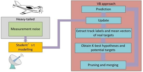
3. MHMTB Filter for a Heavy-Tailed Observation Noise

The MHMTB filter for a heavy-tailed observation noise consists of the following steps.

3.1. Prediction

Given that the potential targets at time step k 1 are
{ T k 1 , i = [ { w k 1 , i e , f k 1 , i e ( x k 1 , i | y 1 : k 1 ) } e = 1 n k 1 , i , r k 1 , i , l k 1 , i ] } i = 1 N k 1
where l k 1 , i , r k 1 , i and n k 1 , i denote the track label, existence probability and sub-item number of target i , respectively; w k 1 , i e and f k 1 , i e ( x k 1 , i | y 1 : k 1 ) denote the weight and PDF of sub-item e of target i , respectively. According to [31,32], f k 1 , i e ( x k 1 , i | y 1 : k 1 ) can be given by
f k 1 , i e ( x k 1 , i | y 1 : k 1 )   = N ( x k 1 , i ; m k 1 , i e , P k 1 , i e ) l = 1 m z { G a m m a ( r k 1 , i l ; α k 1 , i e , l , β k 1 , i e , l ) G a m m a ( g k 1 , i l ; γ k 1 , i e , l , η k 1 , i e , l ) }
where α k 1 , i e , l and γ k 1 , i e , l are the shape parameters; β k 1 , i e , l and η k 1 , i e , l are the inverse scale parameters; and m k 1 , i e and P k 1 , i e denote the mean and covariance of sub-item e of target i .
The predicted potential targets at time step k are
{ T k | k 1 , i = [ { w k | k 1 , i e , f k | k 1 , i e ( x k , i | y 1 : k 1 ) } e = 1 n k 1 , i , r k | k 1 , i , l k | k 1 , i ] } i = 1 N k 1
According to [31,32], the predicted PDF of sub-item e of potential target i , and its predicted existence probability and predicted track label can be given by
f k | k 1 , i e ( x k , i | y 1 : k 1 ) = N ( x k , i ; m k | k 1 , i e , P k | k 1 , i e ) l = 1 m z { G a m m a ( r k , i l ; α k | k 1 , i e , l , β k | k 1 , i e , l ) × G a m m a ( g k , i l ; γ k | k 1 , i e , l , η k | k 1 , i e , l ) }
r k | k 1 , i = p S r k 1 , i ,   l k | k 1 , i = l k 1 , i
m k | k 1 , i e = φ ( m k 1 , i e ) ,   Φ k 1 , i = φ ( x k 1 , i ) x k 1 , i | x k 1 , i = m k 1 , i e ,   P k | k 1 , i e = Φ k 1 , i P k 1 , i e Φ k 1 , i T + Q k 1
α k | k 1 , i e , l = τ ρ α k 1 , i e , l , β k | k 1 , i e , l = τ ρ β k 1 , i e , l , γ k | k 1 , i e , l = τ ρ γ k 1 , i e , l , η k | k 1 , i e , l = τ ρ η k 1 , i e , l
where τ ρ [ 0 , 1 ] is the spread factor.
Given that the potential birth targets at time step k are
{ T k , i b = [ { w k , i b , e , f k , i b , e ( x k , i ) } e = 1 n k , i b , r k , i b , l k , i b ] } i = 1 N k b
where N k b denotes the birth target number; n k , i b , l k , i b and r k , i b denote the given sub-item number, track label and existence probability of birth target i ; and w k , i b , e and f k , i b , e ( x k , i ) denote the weight and PDF of sub-item e of birth target i . According to [31,32], f k , i b , e ( x k , i ) can be given by
f k , i b , e ( x k , i ) = N ( x k , i ; m k , i b , e , P k , i b , e ) l = 1 m z G a m m a ( r k , i l ; α k , i b , e , l , β k , i b , e , l ) G a m m a ( g k , i l ; γ k , i b , e , l , η k , i b , e , l )
where m k , i b , e is the given mean vector; P k , i b , e is the given error covariance matrix; α k , i b , e , l and γ k , i b , e , l are the given shape parameters; and β k , i b , e , l and η k , i b , e , l are the given inverse scale parameters.
In order to track the birth targets, it is necessary to combine the potential birth targets into the predicted potential targets. The predicted potential targets after combining are given by
{ T k | k 1 , i = [ { w k | k 1 , i e , f k | k 1 , i e ( x k , i | y 1 : k 1 ) } e = 1 n k 1 , i , r k | k 1 , i , l k | k 1 , i ] } i = 1 N k | k 1 = { T k | k 1 , i = [ { w k | k 1 , i e , f k | k 1 , i e ( x k , i | y 1 : k 1 ) } e = 1 n k 1 , i , r k | k 1 , i , l k | k 1 , i ] } i = 1 N k 1 { T k , i b = [ { w k , i b , e , f k , i b , e ( x k , i ) } e = 1 n k , i b , r k , i b , l k , i b ] } i = 1 N k b
where N k | k 1 = N k 1 + N k b .

3.2. Update

Given the predicted potential targets in (26), the probability that observation z k j belongs to potential target i is
p i j = e = 1 n k | k 1 , i w k | k 1 , i e S t ( z k j ; h ( m k | k 1 , i e ) , C k , i e P k | k 1 , i e ( C k , i e ) T + R k , r k )
where R k and r k are the scale matrix and the degree of freedom of observation noise, respectively, and C k , i e is given by
C k , i e = h ( x k , i ) x k , i | x k , i = m k | k 1 , i e
The updated weight of sub-item e of potential target i is
w k , ( i j ) e = w k | k 1 , i e S t ( z k j ; h ( m k | k 1 , i e ) , C k , i e P k | k 1 , i e ( C k , i e ) T + R k , r k ) e = 1 n k | k 1 , i w k | k 1 , i e S t ( z k j ; h ( m k | k 1 , i e ) , C k , i e P k | k 1 , i e ( C k , i e ) T + R k , r k )
The updated PDF of sub-item e of potential target i is given by
f k , ( i j ) e ( x k , i | z k j ) = N ( x k , i ; m k , ( i j ) e , P k , ( i j ) e ) l = 1 m z { G a m m a ( r k , i l ; α k , ( i j ) e , l , β k , ( i j ) e , l ) × G a m m a ( g k , i l ; γ k , ( i j ) e , l , η k , ( i j ) e , l ) }
where α k , ( i j ) e , l and γ k , ( i j ) e , l are given by
α k , ( i j ) e , l = 1 2 + α k | k 1 , i e , l ;   γ k , ( i j ) e , l = 1 2 + γ k | k 1 , i e , l
According to the VB technique [31,32], an iteration procedure is required to determine mean vector m k , ( i j ) e , covariance P k , ( i j ) e and inverse scale parameters β k , ( i j ) e , l and η k , ( i j ) e , l . Firstly, the initial parameters for the iteration procedure are given by
m k , ( i j ) e , 0 = m k | k 1 , i e ;   P k , ( i j ) e , 0 = P k | k 1 , i e ;   β k , ( i j ) e , l , 0 = β k | k 1 , i e , l ;   η k , ( i j ) e , l , 0 = η k | k 1 , i e , l ,   n = 0
The iteration procedure consists of Equations (33) to (43).
Λ k , ( i j ) e , n = d i a g { α k , ( i j ) e , 1 β k , ( i j ) e , 1 , n , , α k , ( i j ) e , m z β k , ( i j ) e , m z , n }
a l = γ k , ( i j ) e , l 2 η k , ( i j ) e , l , n + 1 2
b l = γ k , ( i j ) e , l 2 η k , ( i j ) e , l , n + 1 2 t r a c e { Λ k , ( i j ) e , n [ z k j h ( m k | k 1 , i e ) ] [ z k j h ( m k | k 1 , i e ) ] T + C k , i e P k , ( i j ) e , n ( C k , i e ) T }
s l = a l b l + 1 2 ;   l { 1 , , m z }
S = d i a g ( s 1 , , s m z )
K k , ( i j ) e , n = P k | k 1 , i e ( C k , i e ) T [ C k , i e P k | k 1 , i e ( v i , k ) ( C k , i e ) T + ( S Λ k , ( i j ) e , n ) 1 ] 1
m k , ( i j ) e , n = m k | k 1 , i e + K k , ( i j ) e , n ( z k j h ( m k | k 1 , i e ) )
P k , ( i j ) e , n = ( I K k , ( i j ) e , n C k , i e ) P k | k 1 , i e
[ β k , ( i j ) e , 1 , n + 1 β k , ( i j ) e , m z , n + 1 ] = [ β k | k 1 , i e , 1 β k | k 1 , i e , m z ]   +   1 2 Idiag { S [ z k j h ( m k | k 1 , i e ) ] [ z k j h ( m k | k 1 , i e ) ] T + C k , i e P k , ( i j ) e , n ( C k , i e ) T }
η k , ( i j ) e , l , n + 1 = η k | k 1 , i e , l 1 2 [ 1 + Γ ( a l ) Γ ( a l ) log b l s l ] ;   l { 1 , , m z }
n = n + 1
where Γ ( x ) = d ( Γ ( x ) ) d x is the derivative of Γ ( x ) and Idiag(X) is the main diagonal of matrix X.
The iteration procedure ends if m k , ( i j ) e , n m k , ( i j ) e , n 1 2 < τ , where τ is a given parameter. Mean vector m k , ( i j ) e , covariance P k , ( i j ) e and inverse scale parameters β k , ( i j ) e , l and η k , ( i j ) e , l in (30) can be given by
m k , ( i j ) e = m k , ( i j ) e , n ;   P k , ( i j ) e = P k , ( i j ) e , n ;   β k , ( i j ) e , l = β k , ( i j ) e , l , n ;   η k , ( i j ) e , l = η k , ( i j ) e , l , n

3.3. Obtaining K-Best Hypotheses and Potential Targets

The minimization problem in (12) can be recast as a two-dimensional (2-D) assignment problem [26]. The cost matrix of this 2-D assignment is given by C o s t = [ C o s t 1 C o s t 2 C o s t 3 ] ,where
C o s t 1 = [ ln ρ i j ] N k | k 1 × M k
C o s t 2 = [ ln ρ 1 , u ln ρ 2 , u ln ρ N k | k 1 , u ] N k | k 1 × N k | k 1
C o s t 3 = [ ln ρ 1 , 0 ln ρ 2 , 0 ln ρ N k | k 1 , 0 ] N k | k 1 × N k | k 1
Employing the optimizing Murty algorithm [33] to resolve the 2-D assignment problem, we can obtain K-best hypotheses. The K-best hypotheses and total costs of individual hypotheses can be denoted as
H y = [ θ 1 h 1 θ N k | k 1 h 1 θ 1 h K θ N k | k 1 h K ] ;   T o t a l _ C = [ t c h 1 t c h 2 t c h K ]
where θ i h e { 1 , , M k + 2 N k | k 1 } is the column index of matrix C o s t , t c h e is the total cost of hypothesis h e , and i { 1 , , N k | k 1 } and e { 1 , , K } . We may determine whether target i is detected, undetected or disappearing according to index θ i h e . If θ i h e M k , target i is detected and observation z k θ i h e belongs to target i ; if M k < θ i h e M k + N k | k 1 , target i is undetected; and if θ i h e > M k + N k | k 1 , target i is disappearing. The weights of individual hypotheses are given by
w h e = exp ( t c h e ) l = 1 K exp ( t c h l )
We employ Algorithm 1 to acquire the potential targets at time step k . The set of potential targets is
{ T k , i = [ { w k , i e , f k , i e ( x k , i | y 1 : k ) } e = 1 n k , i , r k , i , l k , i ] } i = 1 N k | k 1
where
f k , i e ( x k , i | y 1 : k )   = N ( x k , i ; m k , i e , P k , i e ) l = 1 m z G a m m a ( r k , i l ; α k , i e , l , β k , i e , l ) G a m m a ( g k , i l ; γ k , i e , l , η k , i e , l )
Algorithm 1: Acquiring the potential targets
set b i = 0   for   i = 1 : N k | k 1 , i .
for   l = 1 :   K
for   i = 1 :   N k | k 1
a = θ i h l .
if   a M k
for   e = 1 :   n k | k 1 , i
b i = b i + 1 , w k , i b i = w k , ( i a ) e w h l , f k , i b i ( x k , i | y 1 : k ) = f k , ( i a ) e ( x k , i | z k j ) .
   end
  else if a M k + N k | k 1
for   e = 1 :   n k | k 1 , i
b i = b i + 1 , w k , i b i = w k | k 1 , i e w h l , f k , i b i ( x k , i | y 1 : k ) = f k | k 1 , i e ( x k , i | y 1 : k 1 ) .
   end
  end
 end
end
for   i = 1 :   N k | k 1
n k , i = b i , l k , i = l k | k 1 , i , r k , i = b = 1 n k , i w k , i b , w k , i b = w k , i b / r k , i   for   b = 1 : n k , i .
end
output: { T k , i = [ { w k , i b , f k , i ( x k , i | y 1 : k ) } b = 1 n k , i , r k , i , l k , i ] } i = 1 N k | k 1 .

3.4. Extracting the Track Labels and Mean Vectors of Real Targets

Identical to the approach in [26], if the existence probability of potential target i is greater than ρ τ ,where ρ τ is a given threshold, we identify that this potential target is a real target. Using Algorithm 2 to acquire a set consisting of mean vectors and track labels of real targets, the acquired set can be given by { m k e , l k e } e = 1 N k t where N k t denotes the estimated number of targets. This set is used as the output of the filter.

3.5. Pruning and Merging

Identical to the approach in [26], potential objects with a small existence probability and sub-items with a weak weight should be discarded to decrease the computational burden. For each potential target, the sub-items which are close together should be merged into a sub-item. Algorithm 3 describes the pruning and merging approach where τ 1 , τ 2 and τ 3 are the given thresholds and
α k , i e = [ α k , i e , 1 α k , i e , m z ] ;   β k , i e = [ β k , i e , 1 β k , i e , m z ] ;   γ k , i e = [ γ k , i e , 1 γ k , i e , m z ] ;   η k , i e = [ η k , i e , 1 η k , i e , m z ]
According to Algorithm 3, the residual potential targets after pruning and merging can be given by
{ T k , i = [ { w k , i e , f k , i e ( x k , i | y 1 : k ) } e = 1 n k , i , r k , i , l k , i ] } i = 1 N k
where N k denotes the number of targets. These potential targets are propagated to the next time step.
Algorithm 2: Extracting the track labels and mean vectors of real targets
set e = 0 .
for   i = 1 :   N k | k 1
if   r k , i > ρ τ
e = e + 1 , l k e = l k , i .
b = arg max c [ 1 , , n k , i ] ( w k , i c ) , m k e = m k , i b .
  end
end
N k t = e .
output: { m k e , l k e } e = 1 N k t .
Algorithm 3: Pruning and merging
b = { i = 1 , , N k | k 1 | r k , i > τ 1 } , N k = length ( b ) .
for   i = 1 :   N k
r ^ k , i = r k , b ( i ) , l ^ k , i = l k , b ( i ) , n ˜ k , i = n k , b ( i ) .
{ w ˜ k , i e , m ˜ k , i e , P ˜ k , i e } e = 1 n ˜ k , i = { w k , b ( i ) e , m k , b ( i ) e , P k , b ( i ) e } e = 1 n k , b ( i ) .
{ α ˜ k , i e , β ˜ k , i e , γ ˜ k , i e , η ˜ k , i e } e = 1 n ˜ k , i = { α k , b ( i ) e , β k , b ( i ) e , γ k , b ( i ) e , η k , b ( i ) e } e = 1 n k , b ( i ) .
A = { i = 1 , , n ˜ k , i | w ˜ k , i e > τ 2 } , e = 0 .
 repeat
e = e + 1 , l = arg max c A ( w ˜ k , i c ).
B = { c A | ( m ˜ k , i c m ˜ k , i l ) T ( P ˜ k , i l ) 1 ( m ˜ k , i c m ˜ k , i l ) τ 3 } .
w ^ k , i e = c B w ˜ k , i c , m ^ k , i e = 1 w ^ k , i e c B w ˜ k , i c m ˜ k , i c .
P ^ k , i e = 1 w ^ k , i e c B w ˜ k , i c ( P ˜ k , i c + ( m ˜ k , i c m k , i e ) ( m ˜ k , i c m k , i e ) T ) .
α ^ k , i e = 1 w ^ k , i e c B w ˜ k , i c α ˜ k , i c , β ^ k , i e = 1 w ^ k , i e c B w ˜ k , i c β ˜ k , i c .
γ ^ k , i e = 1 w ^ k , i e c B w ˜ k , i c γ ˜ k , i c , η ^ k , i e = 1 w ^ k , i e c B w ˜ k , i c η ˜ k , i c .
A = A \ B .
 until A =
n ^ k , i = e .
end
output: { { w ^ k , i e , m ^ k , i e , P ^ k , i e , α ^ k , i e , β ^ k , i e , γ ^ k , i e , η ^ k , i e } e = 1 n ^ k , i , r ^ k , i , l ^ k , i } i = 1 N k .
Identical to the MHMTB filter in [26], the proposed filter requires K-best hypotheses to generate the existence probabilities and PDFs of targets at each recursion. Unlike the original MHMTB filter that requires a Gaussian observation noise, the proposed filter obviates this requirement by modeling the heavy-tailed observation noise as a Student’s t distribution. The VB technique is applied in the proposed filter to acquire the approximate posterior distributions of individual targets.

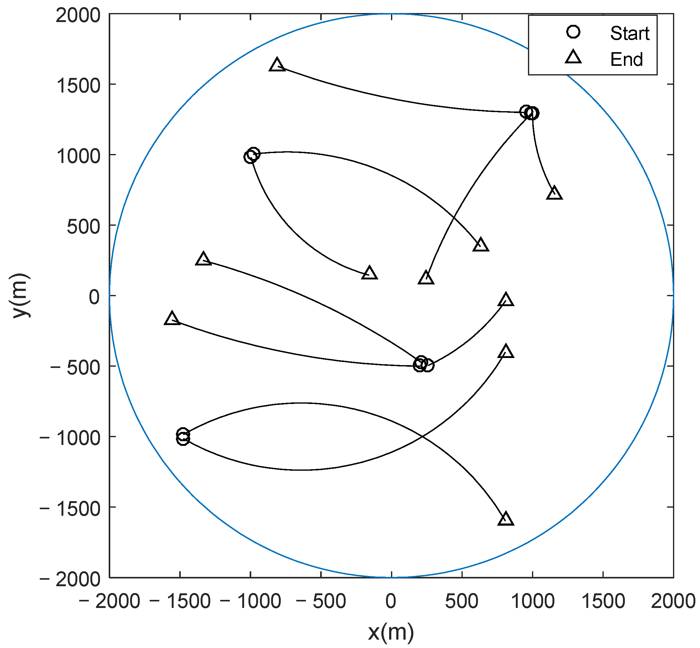
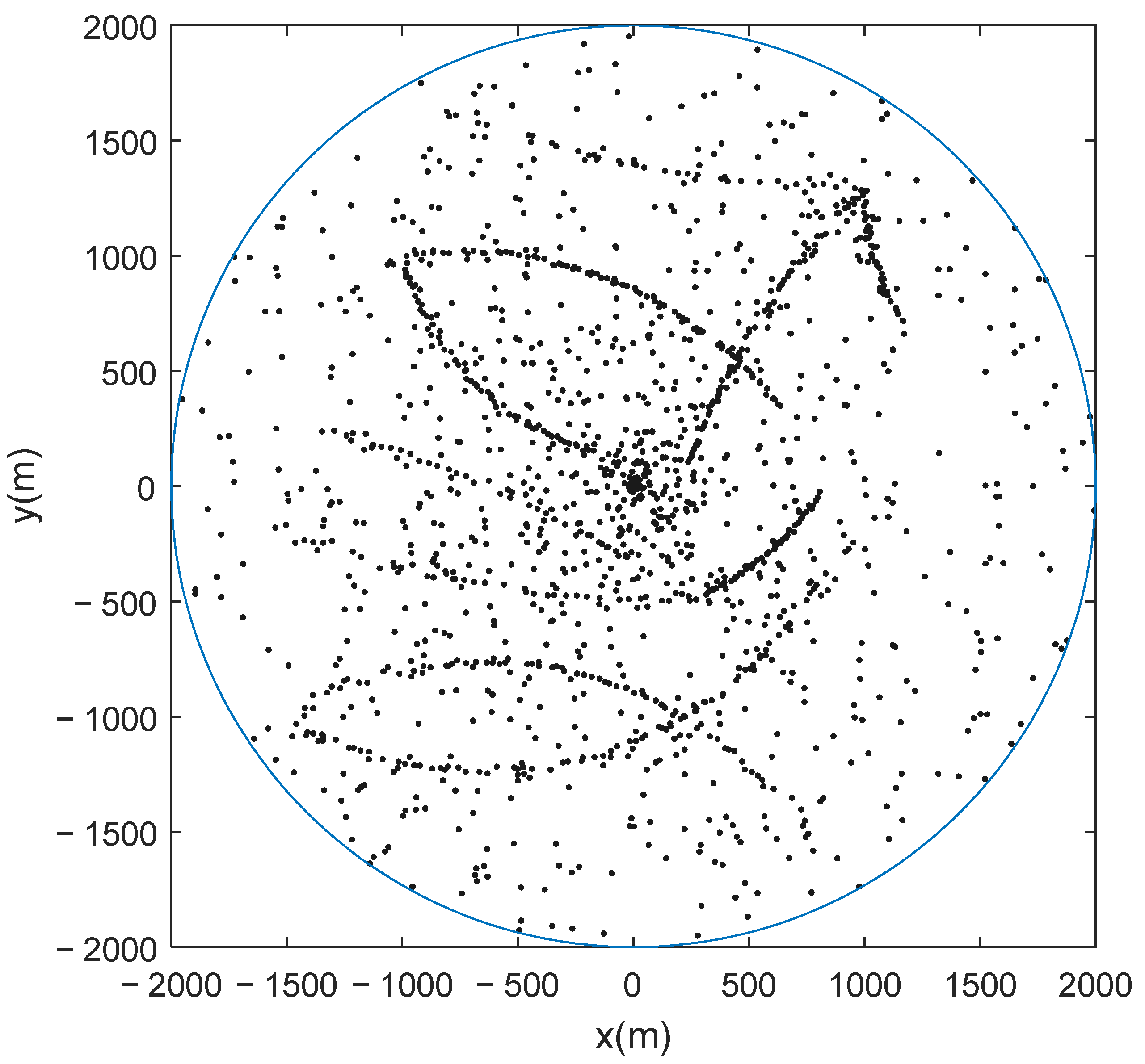
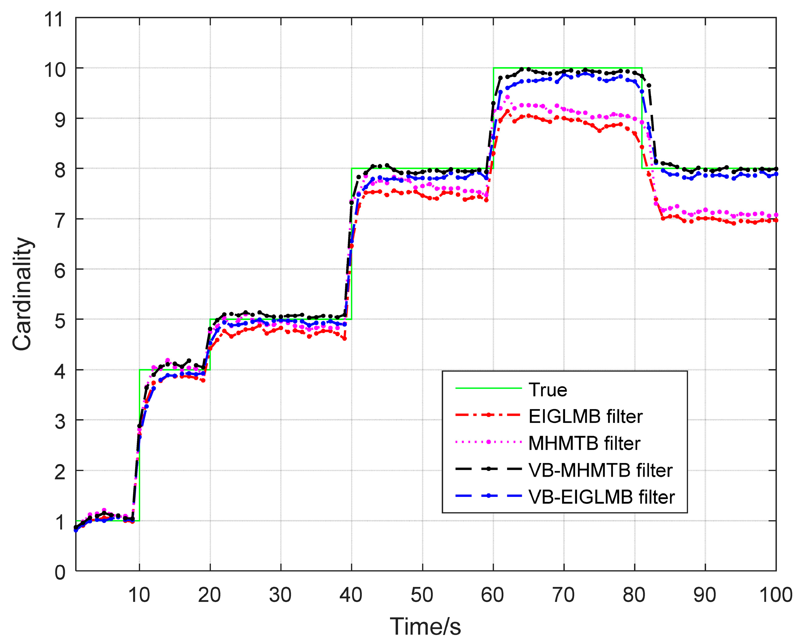
4. Simulation Results

The proposed MHMTB filter for a heavy-tailed observation noise is referred to as the VB-MHMTB filter. The efficient implementation of the GLMB filter (EIGLMB filter) [21] and original MHMTB filter [26] are selected as the comparison objects in this experiment. The VB technique can also be applied to the EIGLMB filter to form an EIGLMB filter for a heavy-tailed observation noise (VB-EIGLMB filter). This filter is also used as a comparison object in this experiment. The performance of the VB-MHMTB filter is evaluated by comparing it with the original MHMTB filter, EIGLMB filter and VB-EIGLMB filter in terms of OSPA(2) error (i.e., the distance between two sets of tracks) [34] and average cardinality error (i.e., the difference between the estimated number of targets and the true number of targets).
For two sets of tracks X = { ξ ( 1 ) , ξ ( 2 ) , , ξ ( m ) } and Y = { τ ( 1 ) , τ ( 2 ) , . τ ( n ) } , if m n , the OSPA(2) error between X and Y is defined as
d p , q ( c ) ( X , Y ; w ) = ( 1 n ( min π Π n i = 1 m d q ( c ) ( ξ ( i ) , τ ( π ( i ) ) ; w ) p + c p ( n m ) ) ) 1 / p
where p and q are the order of the base distance, w is a collection of weights, and it can be given by using a sliding window with the length of window L w . If m > n , then d p , q ( c ) ( X , Y ; w ) = d p , q ( c ) ( Y , X ; w ) . For more detail, we refer the reader to [34]. The parameters used in the OSPA(2) error are given by L w = 5 , c = 100 m and p = q = 2 .
Unlike the OSPA error [35] used to measure the dissimilarity between the two sets of states, the OSPA(2) error is employed to evaluate the difference between the two sets of tracks. Since the above four filters can provide the target trajectory, it is better to select the OSPA(2) error as a metric in the experiment.
The simulated hardware and software environments are Lenovo ThinkPad T430, Windows 7 and Matlab R2015b (32 bits). Figure 1 illustrates a surveillance region where a radar located at [0, 0] observes the ten moving targets. The state of target i at time step k is given by x k , i = [ η k , i x η ˙ k , i x η k , i y η ˙ k , i y ω k , i ] T where η k , i x and η k , i y are its position components; η ˙ k , i x and η ˙ k , i y are its velocity components; and ω k , i is its turn rate. Table 1 gives the initial states of the ten targets and their appearing and disappearing times.
φ ( x k 1 , i ) and Q k 1 in (15) and (22) are given by
φ ( x k 1 , i ) = [ 1 sin ( ω k 1 , i T ) ω k 1 , i 0 1 cos ( ω k 1 , i T ) ω k 1 , i 0 0 cos ( ω k 1 , i T ) 0 sin ( ω k 1 , i T ) 0 0 1 cos ( ω k 1 , i T ) ω k 1 , i 1 sin ( ω k 1 , i T ) ω k 1 , i 0 0 sin ( ω k 1 , i T ) 0 cos ( ω k 1 , i T ) 0 0 0 0 0 1 ] x k 1 , i
Q k 1 = [ q 0 0 0 q 0 0 0 T 2 σ ω 2 ] ; q = [ T 4 / 4 T 3 / 2 T 3 / 2 T 2 ] σ v 2
where T is the scan period; and σ v = 2 ms 2 and σ ω = π / 180 rads 2 are the standard deviations of process noises.
h ( x k , i ) in (16) and (28) is given by
h ( x k , i ) = [ θ ( x k , i ) r ( x k , i ) ] = [ arccos ( η k , i x s x ( η k , i x s x ) 2 + ( η k , i y s y ) 2 ) ( η k , i x s x ) 2 + ( η k , i y s y ) 2 ]
where [ s x s y ] = [ 0 0 ] denotes the position of the radar. The observation noise is assumed to be a Student’s t distribution with degree of freedom r k = 1 and scale matrix R k = [ σ θ 2 0 0 σ r 2 ] , where σ θ = 0.5 π / 180 rad and σ r = 3 m . Set p s = 0.99 , N c = 10 and p D = 0.9 to generate the observations. The simulated observations for a Monte Carlo run are given in Figure 2.
In the simulated experiment, the potential birth objects at each recursion are given by { T k , i b = [ { w k , i b , e , f k , i b , e ( x k , i ) } e = 1 n k , i b , r k , i b , l k , i b ] } i = 1 N k b where N k b = 4 , n k , i b = 1 , w k , i b , e = 1 , r k , i b = 0.03 , l k , i b = [ k i ] and f k , i b , e ( x k , i ) is given by (25) where m k , 1 b , e = [ 1500 0 1000 0 0 ] T , m k , 2 b , e = [ 1000 0 1000 0 0 ] T , m k , 3 b , e = [ 250 0 500 0 0 ] T , m k , 4 b , e = [ 1000 0 1300 0 0 ] T , P k , i b , e = d i a g ( [ 50 ; 50 ; 50 ; 50 ; 6 π / 180 ] ) 2 , α k , i b , e , 1 = α k , i b , e , 2 = 160 , β k , i b , e , 1 = β k , i b , e , 2 = 2300 , γ k , i b , e , 1 = 0.001 , γ k , i b , e , 2 = 160 , η k , i b , e , 1 = 160 and η k , i b , e , 2 = 1 . The parameters used in the VB-MHMTB filter are set to K = 30 , τ ρ = 0.98 , τ = 0.1 , ρ τ = 0.3 , τ 3 = 4 , τ 2 = 10 5 and τ 1 = 10 3 . We perform the four filters for 100 Monte Carlo runs. The results are shown in Table 2 and Figure 3 and Figure 4.
The result in Figure 3 and the data in Table 2 are used to evaluate the performance of the VB-MHMTB filter and other filters. A smaller OSPA(2) error indicates that a filter has a better tracking accuracy, a low cardinality error means that a filter accurately estimates the number of targets, and a larger performing time implies that a filter has a higher computational load. The OSPA(2) errors and cardinality errors in Table 2 and Figure 3 illustrate that the VB-MHMTB filter and the VB-EIGLMB filter perform better than the MHMTB filter and the EIGLMB filter. The reason for this phenomenon is that the MHMTB filter and EIGLMB filter require a Gaussian observation noise. Direct application of the MHMTB filter and EIGLMB filter to a heavy-tailed observation noise leads to a deteriorated filter performance. By using the VB technique to acquire the approximate distributions of individual targets in the case of a heavy-tailed observation noise, the tracking performance of the VB-MHMTB filter and the VB-EIGLMB filter is improved. In terms of the results in Table 2 and Figure 3 and Figure 4, the VB-MHMTB filter outperforms the other filters because it has a smallest OSPA(2) error and provides the most accurate cardinality estimate (i.e., the lowest cardinality error) among the four filters. The performing times in Table 2 reveal that the VB-MHMTB filter requires a significantly lower computational cost than the EIGLMB filter and the VB-EIGLMB filter, and a slightly larger computational cost than the MHMTB filter. The application of the VB technique to the MHMTB filter increases the computational load of the filter.
Effect of spread factor τ ρ : To provide guidance in selecting the spread factor τ ρ , an analysis of the effect of spread factor on the tracking performance of the VB-MHMTB filter is needed. Table 3 illustrates the average OSPA(2) error and cardinality error of the VB-MHMTB filter over 100 Monte Carlo runs for various spread factors to reveal the effect of spread factor τ ρ on the performance of the VB-MHMTB filter. The OSPA(2) error and cardinality error suggest that it is better to select the spread factor τ ρ from the interval [0.93, 1.0].
Effect of picking probability ρ τ : The picking probability is an important parameter in the VB-MHMTB filter and it is needed to provide guidance for the selection of this parameter. The average OSPA(2) and cardinality errors for different picking probabilities are given in Table 4 and reveal the effect of picking probability on the performance of the VB-MHMTB filter. According to the result in Table 4, it is better to choose the picking probability ρ τ from the interval [0.3, 0.6], and the VB-MHMTB filter performs best at ρ τ = 0.4 .
Computational complexity: Identical to the MHMTB filter, the computational complexity of the VB-MHMTB filter is O ( K ( M + 2 N ) 3 ) ,where K is the number of hypotheses, M is the number of observations and N is the number of potential targets. Compared with the MHMTB filter, the VB-MHMTB filter needs an iteration procedure to determine the updated mean vector and covariance of each sub-item. Therefore, it has a higher computational cost than the MHMTB filter.
In above simulation experiments, the number of time steps is 100, i.e., from 1 to 100; the true number of targets or cardinality at each time step is given by the green line in Figure 4; the average number of noise observations (i.e., average clutter number) at each time step is 10; and average clutter density is 7.9577 × 10 4   rad 1 m 1 .

5. Conclusions

In this study, we apply the MHMTB filter to address the MTT problem under heavy-tailed observation noise. By using the Student’s t distribution to model a heavy-tailed observation noise and applying the VB technique to acquire the approximate distributions of individual targets, we proposed a VB-MHMTB filter. Identical to the MHMTB filter, the VB-MHMTB filter propagates the existence probabilities and PDFs of individual targets. The K-best hypotheses acquired by minimizing the negative log-generalized-likelihood ratio are used to establish the existence probabilities and PDFs of targets at each recursion. Experimental results indicate that the VB-MHMTB filter can achieve a better tracking performance than the selected comparison objects because it exhibits a lower cardinality error and a smaller OSPA(2) error. Experimental results also reveal that the VB-MHMTB filter has a significantly lower computational load than the EIGLMB filter and VB-EIGLMB filter, and a higher computational cost than the MHMTB filter.
Tracking multiple maneuvering targets and tracking the extended targets in a real-world environment are potential applications for the proposed filter. This is also a possible research topic in the future.

Author Contributions

Z.L.: Conceptualization, Methodology, Supervision, Writing—original draft preparation. J.L.: Software, Resources. C.Z.: Visualization, Writing—review and editing. All authors have read and agreed to the published version of the manuscript.

Funding

The National Natural Science Foundation of China (No. 62171287) and Science & Technology Program of Shenzhen (No. JCYJ20220818100004008) supported this study.

Data Availability Statement

The data presented in this study are partly available on request from the corresponding author. The data are not publicly available due to their current restricted access.

Conflicts of Interest

The authors declare no conflict of interest.

References

  1. Mahler, R. Statistical Multisource-Multitarget Information Fusion; Artech House: Norwood, MA, USA, 2007. [Google Scholar]
  2. Mahler, R. Advances in Statistical Multisource-Multitarget Information Fusion; Artech House: Boston, MA, USA, 2014. [Google Scholar]
  3. Bar-Shalom, Y. Multitarget-Multisensor Tracking: Applications and Advances–Volume III; Artech House: Boston, MA, USA, 2000. [Google Scholar]
  4. Yang, Z.; Li, X.; Yao, X.; Sun, J.; Shan, T. Gaussian process Gaussian mixture PHD filter for 3D multiple extended target tracking. Remote Sens. 2023, 15, 3224. [Google Scholar] [CrossRef]
  5. Li, Y.; Wei, P.; You, M.; Wei, Y.; Zhang, H. Joint detection, tracking, and classification of multiple extended objects based on the JDTC-PMBM-GGIW filter. Remote Sens. 2023, 15, 887. [Google Scholar] [CrossRef]
  6. Zhu, J.; Xie, W.; Liu, Z. Student’s t-based robust Poisson multi-Bernoulli mixture filter under heavy-tailed process and measurement noises. Remote Sens. 2023, 15, 4232. [Google Scholar] [CrossRef]
  7. Liu, Z.X.; Chen, J.J.; Zhu, J.B.; Li, L.Q. Adaptive measurement-assignment marginal multi-target Bayes filter with logic-based track initiation. Digit. Signal Process. 2022, 129, 103636. [Google Scholar] [CrossRef]
  8. Du, H.; Xie, W.; Liu, Z.; Li, L. Track-oriented marginal Poisson multi-Bernoulli mixture filter for extended target tracking. Chin. J. Electron. 2023, 32, 1106–1119. [Google Scholar] [CrossRef]
  9. Blackman, S.S. Multiple hypothesis tracking for multiple target tracking. IEEE Trans. Aerosp. Electron. Syst. Mag. 2004, 19, 5–18. [Google Scholar] [CrossRef]
  10. Tugnait, J.K.; Puranik, S.P. Tracking of multiple maneuvering targets using multiscan JPDA and IMM filtering. IEEE Trans. Aerosp. Electron. Syst. 2007, 43, 23–35. [Google Scholar]
  11. Mahler, R. Multitarget Bayes filtering via first-Order multitarget moments. IEEE Trans. Aerosp. Electron. Syst. 2003, 39, 1152–1178. [Google Scholar] [CrossRef]
  12. Vo, B.N.; Ma, W.K. The Gaussian mixture probability hypothesis density filter. IEEE Trans. Signal Process. 2006, 54, 4091–4104. [Google Scholar] [CrossRef]
  13. Vo, B.T.; Vo, B.N.; Cantoni, A. The cardinality balanced multi-target multi-Bernoulli filter and its implementations. IEEE Trans. Signal Process. 2009, 57, 409–423. [Google Scholar]
  14. Granstrom, K.; Orguner, U.; Mahler, R.; Lundquist, C. Extended target tracking using a Gaussian mixture PHD filter. IEEE Trans. Aerosp. Electron. Syst. 2017, 53, 1055–1058. [Google Scholar] [CrossRef]
  15. Hu, Q.; Ji, H.B.; Zhang, Y.Q. A standard PHD filter for joint tracking and classification of maneuvering extended targets using random matrix. Signal Process. 2018, 144, 352–363. [Google Scholar] [CrossRef]
  16. Zhang, Y.Q.; Ji, H.B.; Hu, Q. A fast ellipse extended target PHD filter using box-particle implementation. Mech. Syst. Signal Process. 2018, 99, 57–72. [Google Scholar] [CrossRef]
  17. Zhang, Y.Q.; Ji, H.B.; Gao, X.B.; Hu, Q. An ellipse extended target CBMeMBer filter using gamma and box-particle implementation. Signal Process. 2018, 149, 88–102. [Google Scholar] [CrossRef]
  18. Dong, P.; Jing, Z.L.; Gong, D.; Tang, B.T. Maneuvering multi-target tracking based on variable structure multiple model GMCPHD filter. Signal Process. 2017, 141, 158–167. [Google Scholar] [CrossRef]
  19. Vo, B.T.; Vo, B.N. Labeled random finite sets and multi-object conjugate priors. IEEE Trans. Signal Process. 2013, 61, 3460–3475. [Google Scholar] [CrossRef]
  20. Vo, B.N.; Vo, B.T.; Phung, D. Labeled random finite sets and the Bayes multi-target tracking filter. IEEE Trans. Signal Process. 2014, 62, 6554–6567. [Google Scholar] [CrossRef]
  21. Vo, B.N.; Vo, B.T.; Hoang, H.G. An efficient implementation of the generalized labeled multi-Bernoulli filter. IEEE Trans. Signal Process. 2017, 65, 1975–1987. [Google Scholar] [CrossRef]
  22. Cao, C.H.; Zhao, Y.B.; Pang, X.J.; Suo, Z.L.; Chen, S. An efficient implementation of multiple weak targets tracking filter with labeled random finite sets for marine radar. Digit. Signal Process. 2020, 101, 102710. [Google Scholar] [CrossRef]
  23. Bryant, D.S.; Vo, B.T.; Vo, B.N.; Jones, B.A. A generalized labeled multi-Bernoulli filter with object spawning. IEEE Trans. Signal Process. 2018, 66, 6177–6189. [Google Scholar] [CrossRef]
  24. Wu, W.H.; Sun, H.M.; Cai, Y.C.; Jiang, S.R.; Xiong, J.J. Tracking multiple maneuvering targets hidden in the DBZ based on the MM-GLMB Filter. IEEE Trans. Signal Process. 2020, 68, 2912–2924. [Google Scholar] [CrossRef]
  25. Liang, Z.B.; Liu, F.X.; Li, L.Y.; Gao, J.L. Improved generalized labeled multi-Bernoulli filter for non-ellipsoidal extended targets or group targets tracking based on random sub-matrices. Digit. Signal Process. 2020, 99, 102669. [Google Scholar] [CrossRef]
  26. Liu, Z.X.; Chen, W.; Chen, Q.Y.; Li, L.Q. Marginal multi-object Bayesian filter with multiple hypotheses. Digit. Signal Process. 2021, 117, 103156. [Google Scholar] [CrossRef]
  27. Du, H.Y.; Wang, W.J.; Bai, L. Observation noise modeling based particle filter: An efficient algorithm for target tracking in glint noise environment. Neurocomputing 2015, 158, 155–166. [Google Scholar] [CrossRef]
  28. Huang, Y.L.; Zhang, Y.G.; Li, N.; Wu, Z.M.; Chambers, J.A. A novel robust Student’s t-based Kalman filter. IEEE Trans. Aerosp. Electron. Syst. 2017, 53, 1545–1554. [Google Scholar] [CrossRef]
  29. Dong, P.; Jing, Z.L.; Leung, H.; Shen, K.; Wang, J.R. Student-t mixture labeled multi-Bernolli filter for multi-target tracking with heavy-tailed noise. Signal Process. 2018, 152, 331–339. [Google Scholar] [CrossRef]
  30. Zhu, H.; Leung, H.; He, Z.S. A variational Bayesian approach to robust sensor fusion based on Student-t distribution. Inf. Sci. 2013, 221, 201–214. [Google Scholar] [CrossRef]
  31. Li, W.L.; Jia, Y.M.; Du, J.P.; Zhang, J. PHD filter for multi-target tracking with glint noise. Signal Process. 2014, 94, 48–56. [Google Scholar] [CrossRef]
  32. Liu, Z.X.; Huang, B.J.; Zou, Y.N.; Li, L.Q. Multi-object Bayesian filter for jump Markov system under glint noise. Signal Process. 2019, 157, 131–140. [Google Scholar] [CrossRef]
  33. Miller, M.; Stone, H.; Cox, I. Optimizing Murty’s ranked assignment method. IEEE Trans. Aerosp. Electron. Syst. 1997, 33, 851–862. [Google Scholar] [CrossRef]
  34. Beard, M.; Vo, B.T.; Vo, B.N. OSPA(2): Using the OSPA metric to evaluate multi-target tracking performance. In Proceedings of the International Conference on Control, Automation and Information Sciences (ICCAIS), Chiang Mai, Thailand, 31 October–1 November 2017; pp. 86–91. [Google Scholar]
  35. Schuhmacher, D.; Vo, B.T.; Vo, B.N. A consistent metric for performance evaluation of multi-object filters. IEEE Trans. Signal Process. 2008, 56, 3447–3457. [Google Scholar] [CrossRef]
Figure 1. Surveillance region and real trajectories of targets.
Remotesensing 15 05258 g001
Figure 2. Simulated observations.
Remotesensing 15 05258 g002
Figure 3. Average OSPA(2) errors.
Remotesensing 15 05258 g003
Figure 4. Cardinality estimates.
Remotesensing 15 05258 g004
Table 1. Initial state, appearing time and disappearing time of the target.
TargetInitial StateAppearing Time (s)Disappearing Time (s)
1 [ 1000 , 10 , 1300 , 10 , ( 2 π / 180 ) / 8 ] T 1101
2 [ 1000 , 20 , 1000 , 3 , ( 2 π / 180 ) / 3 ] T 10101
3 [ 1500 , 25 , 1000 , 15 , ( 2 π / 180 ) / 2 ] T 10101
4 [ 1500 , 25 , 1000 , 15 , ( 2 π / 180 ) / 2 ] T 10101
5 [ 250 , 11 , 500 , 5 , ( 2 π / 180 ) / 4 ] T 2080
6 [ 1000 , 5 , 1000 , 20 , ( 2 π / 180 ) / 2 ] T 40101
7 [ 1000 , 0 , 1300 , 10 , ( 2 π / 180 ) / 4 ] T 40101
8 [ 250 , 45 , 500 , 0 , ( 2 π / 180 ) / 4 ] T 4080
9 [ 1000 , 45 , 1300 , 0 , ( 2 π / 180 ) / 4 ] T 60101
10 [ 250 , 35 , 500 , 25 , ( 2 π / 180 ) / 4 ] T 60101
Table 2. OSPA(2) errors, cardinality errors and performing times.
FilterEIGLMBMHMTBVB-MHMTBVB-EIGLMB
OSPA(2) error (m)41.711139.608431.291535.6949
Cardinality error0.62570.47480.13300.2174
Performing time (s)92.61593.68167.1489111.2920
Table 3. OSPA(2) error and cardinality error for different τ ρ .
τ ρ 0.900.910.920.930.940.950.960.970.980.991.0
OSPA(2) error34.7933.2432.3031.5331.1530.9931.0530.9731.0531.0031.13
Cardinality error0.1300.1270.1280.1290.1280.1290.1360.1310.1320.1290.137
Table 4. OSPA(2) error and cardinality error for different ρ τ .
ρ τ 0.10.20.30.40.50.60.70.80.9
OSPA(2) error40.6534.5131.7530.5832.1032.3233.0535.4637.44
Cardinality error0.2830.1490.1390.1610.2820.3430.3970.4660.575
Disclaimer/Publisher’s Note: The statements, opinions and data contained in all publications are solely those of the individual author(s) and contributor(s) and not of MDPI and/or the editor(s). MDPI and/or the editor(s) disclaim responsibility for any injury to people or property resulting from any ideas, methods, instructions or products referred to in the content.

