Article

Identifying Winter Wheat Using Landsat Data Based on Deep Learning Algorithms in the North China Plain

1
Collaborative Innovation Center on Forecast and Evaluation of Metcorological Disasters, Nanjing University of Information Science & Technology (NUIST), Nanjing 210044, China
2
China Meteorological Administration Key Laboratory for Climate Prediction Studies, National Climate Center, Beijing 100081, China
3
School of Remote Sensing & Geomatics Engineering, Nanjing University of Information Science & Technology (NUIST), Nanjing 210044, China
*
Author to whom correspondence should be addressed.
Remote Sens. 2023, 15(21), 5121; https://doi.org/10.3390/rs15215121
Submission received: 12 September 2023 / Revised: 19 October 2023 / Accepted: 23 October 2023 / Published: 26 October 2023

Abstract

:
The North China Plain (NCP) represents a significant agricultural production region in China, with winter wheat serving as one of its main grain crops. Accurate identification of winter wheat through remote sensing technology holds significant importance in ensuring food security in the NCP. In this study, we have utilized Landsat 8 and Landsat 9 imagery to identify winter wheat in the NCP. Multiple convolutional neural networks (CNNs) and transformer networks, including ResNet, HRNet, MobileNet, Xception, Swin Transformer and SegFormer, are used in order to understand their uncertainties in identifying winter wheat. At the same time, these deep learning (DL) methods are also compared to the traditional random forest (RF) method. The results indicated that SegFormer outperformed all methods, of which the accuracy is 0.9252, the mean intersection over union (mIoU) is 0.8194 and the F1 score (F1) is 0.8459. These DL methods were then applied to monitor the winter wheat planting areas in the NCP from 2013 to 2022, and the results showed a decreasing trend.

Graphical Abstract

1. Introduction

As the second largest grain crop in China, wheat plays a great meaningful role in ensuring food security and the sustainable utilization of cultivated land [1]. Wheat can be divided into spring wheat and winter wheat, with winter wheat accounting for about 98% of wheat in China [2]. According to the grain statistics from 2019 to 2022 released by the National Bureau of Statistics, the sown area of wheat in China accounted for 20.44%, 20.04%, 20.01% and 19.87% of the total sown area of grain crops [3,4,5,6,7], showing a slow downward trend. In recent years, human activities have brought unprecedented impacts on agricultural production [8,9,10], posing significant threats to the sustainable development of agriculture. The North China Plain (NCP) ranks as one of the largest grain-producing regions in China [11], the dominant planting system in this region is the rotation of winter wheat and summer maize, and winter wheat yield in this region accounts for approximately 75% of total Chinese wheat yield [12]. Simultaneously, the NCP is also one of the regions with the most severe shortage of water resources in the world [13,14]. The contradiction between agriculture and water resources in the NCP is very acute [15,16], it also threatens food security in the NCP. Traditionally, statistical methods have heavily relied on local administrative departments to expend substantial human and material resources for making statistical statements and reporting them step by step or taking a certain proportion of sampling surveys [17,18]. It is not only inefficient but also susceptible to human factors such as omission and misstatement. In contrast, satellite remote sensing has outstanding advantages such as wide coverage, fast data acquisition, high data accuracy, strong macro-monitoring ability and low cost [19]. Thus, using remote sensing to obtain accurate information on the planting area and distribution of winter wheat is of great practical importance [20,21,22].
The prerequisite for obtaining information about the planting area and distribution of crops lies in accurately identifying crops in remote sensing imagery. Table 1 shows previous studies on crop extraction using various remote sensing data. Both Chu et al. [23] and Teluguntla et al. [24] used moderate-resolution imaging spectroradiometer (MODIS) time series data, the former extracted spatial distribution information of winter wheat in the Yellow River Delta, China, and the latter mapped croplands of Australian. Nevertheless, limitations of spatial resolution of the data cause the crop identification results to be coarse and poor for identifying small parcels of farmland, making it difficult to meet application requirements [25,26]. In recent years, Sentinel-1 and Sentinel-2 from the European Space Agency (ESA) have provided good data for crop classification, offering a high spatial resolution of 10 m and a high temporal resolution of 12 days [27]. Van et al. [28] used joint Sentinel-1 radar and Sentinel-2 optical imagery to map eight crop types in Belgium, they found that the synergistic use of radar and optical data in crop classification provided more abundant information, thereby improving classification accuracy compared to optical classification alone. While Sentinel-1 can be observed all day, in all weather conditions, and has strong penetration through clouds, it introduces noise that can easily cause an uncertain impact on crop identification [29]. Furthermore, the available years of Sentinel data are relatively short, rendering them insufficient for meeting the demands of long-term crop mapping. The emergence of the Gaofen (GF) series of satellites provides a very good data source for crop distribution information extraction. You et al. [30] and Ma et al. [31] used the GF-1 satellite with 16 m resolution to extract winter wheat at the county scale and both achieved classification accuracy exceeding 90%. Zhang et al. [32] fused GF-2 imagery to obtain 1 m high-resolution imagery and extracted the spatial distribution of winter wheat by using deep learning (DL) methods, which produced superior results. However, high-resolution imagery is expensive and is not suitable for extracting large regions. At this point, the advantages of medium- and high-resolution satellites become apparent, such as Landsat.
Feature extraction serves as the linchpin for image classification and segmentation. Earlier methods for crop extraction using remote sensing primarily relied on visual interpretation based on textural features and vegetation index based on spectral analysis [33,34]. Liu et al. [35] used a fuzzy decision tree classifier and normalized difference vegetation index (NDVI)-derived climate indicators from MODIS to identify winter wheat, soybean, corn and forage crops in southwestern Ontario, eastern Canada, achieving an overall accuracy of 75.3%. Chen et al. [36] utilized MODIS time series NDVI data to extract the spatial distribution of crops in three northeastern provinces and compared the area derived from the results of crop classification with the statistical data, they obtained correlation coefficients of 0.770, 0.710 and 0.686 for soybean, maize and rice, respectively. While these methods could identify low-level features such as color, shape and texture in images, they could not provide an intuitive semantic description, leading to unsatisfactory classification accuracy [37]. Following advances in machine learning, techniques such as support vector machine (SVM) [38], maximum likelihood classification [39], random forest (RF) [40] and decision tree (DT) have been applied to crop classification [41]. Zheng et al. [42] and Sisodia et al. [39] utilized Landsat imagery, the former employed an SVM to classify nine major crop types within a cropping system, while the latter used a maximum likelihood method for land cover classification, and both studies achieved good result. Wang et al. [43] conducted fine classification of crops by combining feature transformation with RF and found that this combination produced the best classification effect. Sang et al. [44] applied a DT classification method based on the CART (classification and regression tree) algorithm to extract land use information and investigate land use changes in Tianjin. These methods are also shown in Table 1. Unfortunately, these shallow learning algorithms are limited by the network structure. When faced with the complex situation of increasing sample size or sample diversity, these methods cannot adapt, so they cannot express the complex function well [45].
Table 1. Previous research for crop extraction using remote sensing.
ReferenceDataMethodApplication
Chu et al., 2016 [23]MODISVegetation indexCrop mapping
Teluguntla et al., 2017 [24]MODISquantitative spectrum matching technique (QSMT) + Automatic cultivated land classification algorithm based on rules (ACCA)Crop mapping
Van et al., 2018 [28]Sentinel-1, 2RFCrop mapping
You et al., 2016 [30]GF-1Spectral analysisCrop area extraction
Ma et al., 2016 [31]GF-1Image interpretation + GIS analysisCrop area extraction
Zhang et al., 2018 [32]GF-2A hybrid structure convolutional neural network (HSCNN)Crop mapping
Liu et al., 2016 [35]MODISA fuzzy decision tree classifier + vegetation indexCrop classification
Chen et al., 2012 [36]MODISSpectral analysisCrop classification
Sisodia et al., 2014 [39]Landsat ETM+Supervised maximum likelihood classification (MLC)Land cover classification
Zheng et al., 2015 [42]Landsat OLISupport vector machine (SVM)Crop classification
Wang et al., 2022 [43]WHU-HI datasetFeature transform combined with random forest (RF)Crop classification
Sang et al., 2019 [44]Landsat TM, OLIClassification and regression trees (CART)Land use change
For the past few years, DL methods have been widely applied in geoscience, particularly for land cover classification and object identification [46]. DL can effectively process various types of imagery, including optical, radar, hyperspectral and multispectral imagery [47,48]. DL is adept at learning different levels of features in imagery and clearly distinguishing spectral and spatial features of various objects [49], and then extracting different land cover types, such as road extraction [50], building extraction [51] and water extraction [52]. Compared with the traditional visual interpretation and vegetation index methods, the DL methods do not need to define rules for specific tasks in advance [53] and the neural network can automatically learn the deep features from the input image. The DL methods benefit from a deeper network level and can express complex functions well compared to machine learning. The emergence and development of DL have promoted the solution of the problems left by traditional methods. As an important branch of DL, convolution neural networks (CNNs) have the advantage that neurons in the same layer share weight values, which results in a lower number of parameters compared to a fully connected network. The result is a reduction in the complexity of the network model [54,55] and an improvement in the computational efficiency and generality of the model. Following this, a variety of CNN-based segmentation models have been developed, such as U-Net [56], SegNet [57], Deeplab [58], and more. With its impressive feature learning capabilities, CNN models have been successfully and widely used in crop classification scenarios. Wei et al. [27] developed an adapted U-Net for large-scale rice mapping, which mined spatio-temporal features of rice from a multi-temporal dataset to achieve feature segmentation, and improved the accuracy of rice mapping. Kavita et al. [59] used a CNN for crop identification on an Indian pine tree dataset and achieved a high accuracy of 97.58%. Xie et al. [60] used GF1 satellite imagery to classify 70 smallholder agricultural landscapes in Heilongjiang, China, and showed that CNNs are better able to differentiate between spectrally similar crop types through the effective use of spatial information.
Over the past decade, CNNs have been a mainstream semantic segmentation method within the realm of DL. Nevertheless, the localized nature of the convolution operations makes it difficult to obtain the global context features directly based on CNNs [61]. In contrast, the Vision Transformer (ViT) has great potential in long-term dependency modeling. It uses a transformer structure as a feature extractor to process image identification tasks and achieves excellent results in semantic segmentation [62]. Feng et al. [63] combined the Swin Transformer with a Gabor filter and applied it to the classification task of remote sensing imagery. The results demonstrated that ViT exhibits a marginally superior accuracy in comparison to CNNs under the condition of using pre-training. This confirms that the transformer models possess strong feature extraction capability and hold promising potential in the domain of image processing.
This study aims to use a combination of remote sensing monitoring methods and DL technology to accurately identify winter wheat in the NCP, while also monitoring changes in winter wheat planting areas from 2013 to 2022. The main contributions of this work are as follows. First, we developed a winter wheat sample dataset based on the phenological characteristics of winter wheat in the NCP using vegetation index and visual interpretation. Subsequently, we used six DL methods and the RF method to identify winter wheat. Lastly, we monitored the distribution of winter wheat and the changes in planting areas in the NCP from 2013 to 2022. Identifying and monitoring winter wheat using Landsat data has high accuracy and efficiency, helping to promote the implementation of precision agriculture.

2. Materials and Methods

2.1. Study Region

The NCP (32°08′N to 40°24′N, 112°50′E to 122°40′E) is situated in the eastern part of China (Figure 1). It experiences an average annual temperature of 14 °C and receives an annual precipitation ranging from 500 mm to 1000 mm [64]. The NCP belongs to a temperate continental monsoon climate, characterized by simultaneous rainfall and high temperatures; the soil is fertile and is well suited to the growth of wheat, maize, soybeans and other crops. Winter wheat is sown from early to middle October and harvested in June of the following year, while summer maize is sown in middle to late June and harvested in September of the same year [65]. Details of the major crop calendar in the NCP can be found in Figure 2.

2.2. Data

2.2.1. Landsat Imagery

In this study, we used data from Landsat 8 operational land imagery (OLI) and Landsat 9 operational land imagery 2 (OLI-2), with a time resolution of 16 days. Due to the absence of panchromatic bands in Landsat 5, it is difficult to annotate winter wheat. Additionally, Landsat 7 suffers from data stripe loss issues, despite attempts to rectify these gaps using interpolation methods, this adversely affects data quality. We used four bands from Landsat 8 and Landsat 9, including the red, green and blue bands with a spatial resolution of 30 m, as well as the panchromatic band with a spatial resolution of 15 m. We used a total of 13 Landsat images, which have fewer clouds and better clarity, covering a period from 2013 to 2022. As winter wheat has a large biomass at the jointing and heading period, it is easy to identify on remote sensing imagery, so we used remote sensing imagery from 1 April to 20 May of each year. The information on the images used is shown in Table 2. We selected images of different periods and different spatial regions, in order to make the winter wheat samples have temporal and spatial generalization in the NCP. This approach enhances the capabilities of the winter wheat identification model against interference.

2.2.2. Data Pre-Processing

In accordance with the different phenological characteristics of winter wheat in different periods of the NCP, we first extracted a preliminary winter wheat distribution map from the Google Earth Engine (GEE) based on NDVI and normalized burn ratio (NBR) thresholds. The threshold extraction map is then used as auxiliary data to annotate winter wheat, which can help to correctly distinguish winter wheat fields in remote sensing imagery during visual interpretation.
Before annotating winter wheat through visual interpretation, we pre-processed the selected 13 Landsat images, including radiometric calibration and atmospheric correction. To obtain higher-resolution model inputs, we fused the three multispectral bands with the panchromatic band, resulting in multispectral data with a spatial resolution of 15 m.
We manually annotated the Landsat imagery and then filtered the labels to ensure that the positive winter wheat samples made up the majority of the label map. Next, we unified the size of all images and labels to 256 × 256. Finally, we obtained a total of 9956 samples of winter wheat in our dataset. We partitioned the dataset into three subsets, 80% for training samples, 10% for validation samples, and the remaining 10% for test purposes to evaluate the winter wheat identification model. Figure 3 shows a portion of the winter wheat dataset and their corresponding properties. It includes large contiguous farmlands, farmlands interlaced with buildings, and farmlands with surrounding water bodies.

2.3. Methods

The research in this study is structured into six steps, illustrated in Figure 4. The first step involves data selection and pre-processing. In the subsequent phase, we create the winter wheat threshold extraction map using GEE and annotate each Landsat image combined with visual interpretation. In the third step, the dataset is randomly divided. The fourth step is to build winter wheat identification models, including DL models and traditional RF models, and then train each model. In the fifth step, the identification effect of winter wheat of each model was evaluated qualitatively and quantitatively. Finally, changes in winter wheat planting area will be monitored, and the best model will be used to draw the distribution map of winter wheat in the NCP from 2013 to 2022.

2.3.1. Random Forest Classifier

RF is an integrated learning method based on decision trees proposed by Breiman [66], which is commonly applied to address classification and regression problems [67]. Each decision tree of the RF classifier is independent of each other and does not correlate. For each input sample, decision trees will vote on it, and finally, all decision trees jointly determine the optimal classification result of the sample. Compared to other classifiers, RF solves the problem of overfitting by training multiple trees and also has the advantage of being less affected by outliers [68,69], all due to its integrated structure. In the parameter settings, we set the number of estimators to 20, the maximum number of features to “sqrt”, and the bootstrap parameter to “True” by default. We used the Gini coefficient as the evaluation criterion and kept the minimum number of leaf samples and the minimum number of split samples at their default values.

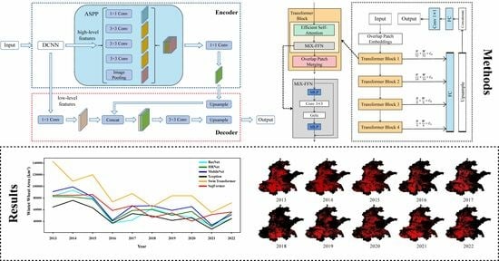
2.3.2. Deeplabv3+ and Improvement

We used the Deeplabv3+ model proposed by the Google team in 2018 [70], which is a typical supervised learning classification approach. The original backbone network in the Deeplabv3+ model is the Xception network. In this study, we added four other backbone networks to the original base, including three CNNs, ResNet, HRNet, MobileNet, and the Swin Transformer network. By skipping the connections of the next layer of neurons and connecting another layer, the ResNet weakens the strong connection between each layer, alleviating problems such as gradient disappearance, gradient explosion and network degradation. The HRNet uses a parallel approach to connect the high-resolution network with the low-resolution network to avoid information loss, always maintains high-resolution features and has strong feature representation ability. The Xception replaces the convolution operation used in the original network with deep separable convolution, further improving the accuracy without increasing its complexity [71,72]. The Swin Transformer proposes a hierarchical network structure so that the model can flexibly process images of different scales [73]. In addition, it adopts window self-attention to reduce the computational complexity. This model can produce satisfactory results in tasks such as instance segmentation, semantic segmentation and object detection [74].
Figure 5 illustrates the network structure of the improved Deeplabv3+. This model comprises an encoder and a decoder. Firstly, the images were fed into the deep convolutional neural networks in the encoder, and 5 feature extraction backbone networks were used for feature extraction. This produces two sets of effective feature layers, one consisting of low-level feature layers and the other containing high-level feature layers. For high-level feature layers, Atrous Spatial Pyramid Pooling (ASPP) [75] was introduced. It captures multi-scale information through the use of different atrous rates, expanding the receptive field of the network so that multi-scale features can be extracted. Next, the feature layers extracted by atrous convolution are stacked and a 1 × 1 Conv was used to adjust the number of channels [76]. Finally, we obtained high-level semantic features in the encoder part. In the decoder part, we first used 1 × 1 Conv to adjust the number of channels for low-level semantic features. At the same time, high-level semantic features were upsampled, and the two results were concatenated to complete feature fusion, and then 3 × 3 Conv was used to extract features from the fusion results. Finally, the output image was resized to match the input image.

2.3.3. SegFormer

The SegFormer [77] is a supervised learning semantic segmentation model based on a transformer structure, comprising an encoder and a decoder. It differs from the Swin Transformer in that it removes the position coding so that the low-resolution pre-training model can be applied to the high-resolution downstream tasks. Figure 6 illustrates the SegFormer framework.
  • SegFormer Encoder
We input 256 × 256 × 3 images into the hierarchical transformer encoder. This encoder section comprises four transformer blocks with identical architectures, designed to produce both high-resolution coarse features and low-resolution fine features. As opposed to ViT, which produces a single-resolution feature map, SegFormer aims to produce multiple levels of features, similar to a CNN, for the input images. This method usually makes the pixel classification more accurate and the segmentation effect of details such as edges more refined, thus leading to improved semantic segmentation performance.
Each transformer block consists of three parts: the efficient self-attention layer, the mix feed-forward network (Mix-FFN) layer and the overlapping patch merging layer [77]. Among these components, efficient self-attention introduces sequence reduction based on the ordinary self-attention structure to reduce computational complexity. Mix-FFN uses a 3 × 3 Conv directly in the feed-forward network (FFN), which helps mitigate the impact of zero-padding on the loss of position information [78]. This alleviates the problem of ViT accuracy degradation in situations where the test resolution differs from the training resolution [79]. To preserve local connections between patches, an overlapping patch merging process is used, and we can obtain feature graphs with resolutions of {1/4, 1/8, 1/16, 1/32} of the original input size.
  • SegFormer Decoder
The SegFormer decoder comprises a multilayer perceptron (MLP) and operates through a four-step process. First, four feature maps of different resolutions are input into the MLP layer, and then the dimensions of the channels are unified. Second, the feature maps are upsampled to 1/4 of the original map using bilinear interpolation and then merged [80]. Next, the merged features are fused with an MLP layer. In the end, another MLP layer is used to predict the fused features for semantic segmentation of images, and the size of the predicted result P is H 4 × W 4 × N C , where N C is the category.

2.4. Evaluation Metrics

We evaluated various models using several metrics, including accuracy, precision, mean intersection over union (mIoU), recall, F1 score (F1) and training time. Accuracy indicates the ratio of the number of correctly classified samples to total samples. Precision reflects the probability of actual positive samples among all predicted positive samples. The mIoU indicates the ratio of the intersection and union of ground truth and predicted values. Recall indicates the probability that the predicted positive sample is in the actual sample. The F1 score takes into account both precision and recall in a comprehensive way to evaluate the classification results. These indexes are all calculated from a confusion matrix, which is composed of true positives (TP), true negatives (TN), false positives (FP) and false negatives (FN) [81]. The calculation equations for these indexes are shown below [82].
  Accuracy =   TN + TP TN + TP + FN + FP
Precision =   TP TP + FP
mIoU =   TP TP + FP + FN
Recall =   TP TP + FN
F 1 = 2   ×   Precision   ×   Recall Precision + Recall

2.5. Experimental Setup

During the training process of these DL models, we adopted a consistent parameter configuration, which included learning rate, training epoch, loss function and optimizer type. We set 400 epochs for each network in our experiments, with 124 iterations within each epoch. The stochastic gradient descent (SGD) method was selected for weight optimization. We set the batch size to 64, with the weight_decay of 0.01, and the momentum of 0.9. After several experiments, we decided on 0.01 as the optimal learning rate for training this model. In addition, we selected step mode as the learning rate scheduler policy and binary cross entropy was used as the loss function. For all experiments, we utilized a Linux system equipped with a GPU, NVIDIA 9.0, and 128 GB of memory, configured with the Pytorch 1.7.0 environment. Furthermore, we used the same dataset in all experiments.

3. Results

In an attempt to discuss the uncertainty of winter wheat identification, we compare the performance of various DL methods with a traditional method, considering the training efficiency, evaluation metrics and identification results of these methods. After that, we use all DL methods to monitor the changes in winter wheat planting area in the NCP from 2013 to 2022 and then select the best-performing method to map the spatial distribution of winter wheat.

3.1. Training Efficiencies

Figure 7 shows the loss curve in the training process of each model. In a semantic segmentation model, the loss function calculates the discrepancy between the predicted results and the actual results, which enables the weight and model to be continuously optimized. When the loss decreases rapidly and becomes more stable over time, it indicates that the model fit is better. It can be seen from Figure 7 that the SegFormer has the lowest initial loss value, followed by ResNet, HRNet, MobileNet, Xception and Swin Transformer. In the first 10 epochs, the loss curves of each model show a rapid downward trend. Around the 30th epoch, the loss value of HRNet was reduced to the same level as ResNet. Simultaneously, the loss value of the SegFormer continued to decrease and the gaps with the other models gradually widened. The SegFormer initially achieved the fastest reduction to the lowest loss value, while the other models eventually converged, although there were still persistent fluctuations. Therefore, the SegFormer has the fastest convergence rate and the best fitting effect of all the models.
The training times of all models are summarized in Table 3. The RF uses fewer parameters and is simple to implement, so it has the shortest training time. On the other hand, the Swin Transformer has the longest train time, more than 40 h, almost twice as long as SegFormer and four times as long as MobileNet, because it is based on numerous parameters, making it difficult to train. Although the training time of SegFormer is not the shortest among all DL models, it is second only to MobileNet and Xception. However, the SegFormer converges faster, has lower loss values and is smoother during training than the previous two models. Therefore, the investment of time in model performance improvement is well justified.

3.2. Winter Wheat Crop Identification

We employ accuracy, precision, mIoU, recall and F1 score to evaluate the performance of different models in winter wheat identification. The metrics for all the methods are listed in Table 4, with the best values being highlighted in bold. Of all the methods, SegFormer has the highest accuracy value of 0.9252, followed by HRNet, ResNet, MobileNet, Xception, Swin Transformer and RF. Their accuracy values are 0.9005, 0.8960, 0.8911, 0.8693, 0.8484 and 0.6732, respectively. The accuracy indicates the proportion of correctly classified winter wheat samples and correctly classified background samples in the total sample, so the metrics do not adequately illustrate the high performance of the model in the winter wheat identification task.
The winter wheat precision represents the probability of there actually being winter wheat samples among all predicted samples. The SegFormer has the highest precision (0.8382), followed by the HRNet (0.8051) and the RF has the lowest precision (0.5809). Despite the fact that the Swin Transformer has the lowest precision of all the DL models, it still outperforms the RF. Recall of winter wheat identification refers to the probability that the actual winter wheat samples are predicted to be winter wheat samples. The recall values from high to low are the SegFormer, HRNet, ResNet, MobileNet, Xception, Swin Transformer and RF methods with values of 0.8538, 0.7901, 0.7885, 0.7671, 0.7264, 0.7155 and 0.4304, respectively. In particular, the recall value of RF is much lower than other models.
The mIoU is used to measure the similarity between predicted results and real labels. The higher the value, the better the model performs. From Table 4, we can see that the SegFormer has the highest mIoU value of 0.8194, indicating that this method outperforms others for identifying winter wheat. The mIoU values of the HRNet, ResNet, MobileNet, Xception, Swin Transformer and RF methods are 0.7698, 0.7592, 0.7522, 0.7104, 0.6612 and 0.4962, respectively. Compared with accuracy and recall rate, mIoU can better reflect model performance. For example, the recall value of Swin Transformer and Xception are very close, but the mIoU value of them is significantly different. The F1 score of winter wheat identification comprehensively considers precision and recall and serves as a measure of the stability of the model performance and its ability to generalize predictions. The SegFormer has high precision and high recall, indicating that both positive and negative classes are predicted correctly. The F1 score of SegFormer is 0.8459, which ranks first, followed by the HRNet with the F1 score of 0.7975, which is about 5% lower than that of SegFormer, while the result of the traditional RF is the worst, with the F1 score of about 35% lower than that of the highest SegFormer. This result indicates that the SegFormer performs well among all models.
Considering accuracy, precision, mIoU, recall and F1 comprehensively, the SegFormer model ranked first among all the models. Consequently, our conclusion is that the SegFormer performed best in the winter wheat identification task in our study. This may be due to the use of multi-scale feature fusion in the SegFormer model. This capability allows the model to capture high-resolution fine features and low-resolution coarse features simultaneously, thereby optimizing segmentation results. Secondly, in terms of performance indicators, the gap between DL networks is small, with the exception of Swin Transformer. In addition, the Swin Transformer performs substantially lower than that of SegFormer, even though both are based on the transformer structure. Specifically, the mIoU of Swin Transformer is about 16% lower than that of SegFormer, and the difference between the F1 score of the two is about 18%. The Swin Transformer performs worse than CNNs under the Deeplabv3+ semantic segmentation framework, which may be because its feature extraction capability as a backbone network is not as good as other CNNs in our winter wheat extraction task. We found that the difference in performance between the traditional RF and these DL networks is very significant, the main reason being that RF is a shallow learning algorithm that is limited by network structure. For the complex task of winter wheat identification in remote sensing imagery, especially in the NCP where there are many types of crops and the planting structure is complex, the advantages are not obvious. As a result, RF cannot produce good classification results.
With the exception of using quantitative evaluation indicators, we compared and analyzed the prediction results of various typical winter wheat types, thereby providing a more comprehensive evaluation of each model. The identification results of various distribution types of winter wheat obtained by several methods are shown in Figure 8. Among them, the first column is the original Landsat imagery, the second column is the winter wheat label, and the third to the ninth columns are the identification results of ResNet, HRNet, MobileNet, Xception, Swin Transformer, SegFormer and RF methods. The first and second rows are of the continuous distribution type, the third and fourth rows are winter wheat interleaved with the building, and the last two rows are winter wheat distributed near water bodies. In Figure 8, the red regions indicate the identified winter wheat fields and the black regions indicate the background.
As can be seen in Figure 8, the SegFormer can identify winter wheat well, whether it is a large area of farmland or a small area of farmland, buildings and roads can also be clearly distinguished from the winter wheat field. Especially regarding edge details, the identification results of SegFormer surpass those of other models and are closely aligned with the ground truth. The ResNet, HRNet and MobileNet were slightly inferior to SegFormer in terms of detail performance. The Xception and Swin Transformer have a poor ability to identify details, for some small plots of farmland, these two models have the problem of missed identification. The boundary of farmland in the identification results of these two models are fuzzy, especially the results of Swin Transformer have no obvious outline, resulting in a large number of high-resolution spatial information being lost. The RF method always ignores the road between the winter wheat fields and shows more misidentifications. When winter wheat fields are distributed near water bodies such as rivers and ponds, etc., the RF method misidentifies large water bodies as winter wheat, which can be seen from the fifth and sixth rows in Figure 8. In addition, it is evident from the identification results presented in the fifth row of Figure 8, that when the spectral characteristics of water are highly similar to those of winter wheat, the ResNet, MobileNet, Xception and Swin Transformer are prone to misclassification in remote sensing imagery. In contrast, the HRNet and SegFormer models are effective in mitigating the influence of water. In conclusion, DL methods can identify winter wheat with different distribution types more accurately compared to machine learning methods. Although both methods have some disadvantages, the SegFormer model has the best effect in the winter wheat identification task.

3.3. Temporal and Spatial Variation Characteristics of Winter Wheat in the North China Plain

We intended to use six DL methods to plot the curve illustrating the alteration of the winter wheat planting area from 2013 to 2022. Due to the fact that the RF method easily identified water bodies as winter wheat, we do not consider this machine learning method here. Due to the large extent of the NCP, it is difficult to obtain images simultaneously, so we obtained Landsat data of the entire NCP by mosaicing satellite images from various acquisition dates and positions using GEE. We cut Landsat imagery of the NCP from 2013 to 2022 into 256 × 256 image blocks and fed these images into the trained DL models for prediction. Subsequently, these predictions were mosaicked together to generate distribution maps of winter wheat planting areas for each year. Eventually, the planting area was obtained by calculating the number of winter wheat pixels.
Figure 9 shows the temporal trend of the winter wheat planting area in the NCP from 2013 to 2022, obtained via ResNet, HRNet, MobileNet, Xception, Swin Transformer and SegFormer. From 2013 to 2022, the winter wheat planting area shows a downward trend globally, but there are fluctuations locally. As a consequence of the discrepancies in the performance of various DL models for identifying winter wheat tasks, there are also slight diversities in the trend of area changes. For the SegFormer, the planting area decreased by approximately 2.9 × 10⁴ km2 from 2013 to 2022. For the ResNet, HRNet, MobileNet, Xception and Swin Transformer, the reduced winter wheat areas are 3.9 × 10⁴, 2.8 × 10⁴, 4.0 × 10⁴, 2.0 × 10⁴ and 7.1 × 10⁴ km2, respectively. In particular, the Swin Transformer consistently identifies a greater amount of winter wheat planting area than the other models. This may be attributed to the model erroneously identifying other land types as winter wheat, such as water bodies, resulting in a higher identified area value. Nevertheless, the overall trend of each model is relatively consistent, which is beneficial for us in order to understand the changing trend of winter wheat planting areas in the NCP during the previous decade.
Based on the aforementioned analysis, we can conclude that the SegFormer model displays the most effective identification capabilities for winter wheat fields. Therefore, we select this model to explore the temporal and spatial distribution characteristics of winter wheat in the NCP during 2013–2022, as shown in Figure 10, where the red regions indicate the winter wheat. From the perspective of spatial distribution, winter wheat is primarily sown across the central, western and southern parts of the NCP. From the perspective of administrative division units, winter wheat is predominantly distributed throughout Kaifeng, Shangqiu and Zhoukou in the eastern part of Henan Province; Anyang, Xinxiang, Hebi and Puyang in the north of Henan Province; Shijiazhuang, Xingtai and Hengshui in central Hebei Province; and Suzhou, Huaibei, Haozhou, Fuyang, Huainan and Bengbu in the north of Anhui Province. On the time scale, the planting area of winter wheat demonstrated a consistent decline in the NCP during 2013–2017, especially in the south of the NCP. In both 2018 and 2019, a pronounced reduction in the area of winter wheat cultivation was observed. Among these reductions in 2018 and 2019, the decrease in the winter wheat planting area in central Hebei Province and northern Henan Province was also attributed to cloud interference in the Landsat images used for these areas, which resulted in the model’s inability to effectively identify winter wheat targets in remote sensing imagery. From 2020 to 2022, the planting area in the southern NCP gradually shrank. In general, there was a decreasing trend observed in the planting area of winter wheat in the NCP from 2013 to 2022.

4. Discussion

The NCP is one of the most important grain-producing areas in China, and timely monitoring of the area planted with winter wheat in the region plays a crucial role in ensuring food security [83]. However, too much statistical work is undoubtedly inefficient and uneconomical [84]; there are even cases of omission. In this study, the combination of deep learning and remote sensing provides an optimal way for obtaining spatial distribution maps of crops. We obtained a spatial distribution map of winter wheat in the NCP with a resolution of 15 m, while previous studies have not obtained a winter wheat map with a higher resolution. Our results have the advantage of high spatial resolution and are less affected by mixed pixels and more accurate. Moreover, our study enables the determination of planting areas one or two months before the maturity of winter wheat, and provides valuable information for early yield predictions.
With the continuous development of smart agriculture, DL technology is gradually being applied to various fields of agriculture, and crop identification is the basis of refined agricultural management. The DL methods we used outperformed the RF method when identifying winter wheat, and the SegFormer model has the most outstanding performance among all DL methods. A possible reason is that the transformer structure can capture a variety of long-term dependencies within the input sequence. In contrast, CNNs can only capture local information but may struggle with long-range dependencies [85]. In addition, the SegFormer model stands out because of its abandonment of position coding. This means that the resolution discrepancy between training and test images has minimal impact on the model performance. Consequently, the winter wheat identification model can quickly adapt to different resolutions, allowing the input of higher-resolution imagery for prediction in future research. However, we found a significant performance gap between SegFormer and Swin Transformer, with the former requiring only half the training time of the latter, while mIoU outperformed the latter by about 16 percentage points. This may be due to the Swin Transformer being a common backbone network under the Deeplabv3+ framework not being able to achieve maximum performance. Thus, in order to improve its performance, it is necessary to construct a suitable semantic segmentation architecture according to its structural properties in future work [86]. In brief, our results confirm that DL methods are highly effective at accurately identifying winter wheat fields, providing a more precise representation of winter wheat distribution, and compensating for the shortcomings of manual statistics. Therefore, the use of SegFormer for crop identification is a reliable choice.
Additionally, the SegFormer model we used has certain transferability because the phenological characteristics and growth patterns of the same crop in different regions are the same or very similar [87]. At the same time, in order to make the transferred model have a better effect, we can use transfer learning technology to transfer the SegFormer model to the target region, with the help of a small number of winter wheat samples from this region [27], we can add more iterative training to the model to achieve a better identification effect.
From the temporal trend of the winter wheat planting area in the NCP, it is evident that the winter wheat planting area in the region exhibited fluctuating changes during the period from 2013 to 2022, showing a general decreasing trend. The reduction in winter wheat planting area in the NCP is mainly influenced by human activities, with three main possible factors:
(1)
With the rapid development of the social economy, China is experiencing rapid urbanization, and a significant amount of farmland on the outskirts of cities has been occupied, which may also be a reason for the gradual reduction in winter wheat area [88].
(2)
In addition, the limited rainfall and the high demand for irrigation in agriculture result in the over-exploitation of groundwater. This creates a conflict between agriculture and water resources, limiting winter wheat production to some extent [89,90].
(3)
The decline of winter wheat cultivation around settlements is also associated with the adjustment of the cropping structure, where many arable lands have been repurposed to cultivate economically efficient cash crops such as vegetables, flowers and medicinal herbs, particularly in the vicinity of towns [91].
Despite our identification result achieving high accuracy, some limitations and uncertainty still exist, as shown below.
Firstly, due to the extensive coverage of the study region, ensuring the availability of images for every region during the winter wheat jointing and heading period is challenging. In cases where images are not available, we must resort to selecting images with the closest dates. However, this may result in deviations ranging from half a month to one month or even longer, which might cause the winter wheat area identified by our model to slightly deviate from the actual area. In addition, the presence of cloud cover or image noise in images can complicate the identification of ground objects, further adding to the challenges. From the above two points, it is evident that the quality of remote sensing imagery plays a significant role in the accuracy of our results. Therefore, in future work, we can improve data quality by integrating multi-source remote sensing data, making imagery available at all stages of crop growth. This will enable us to achieve widespread and precise crop extraction.
Another potential impact is that, while the seasonal variation of winter wheat is relatively consistent across most provinces, there are subtle differences in the phenological characteristics of winter wheat among different provinces [92,93]. These differences might be due to factors such as winter wheat varieties, planting dates and irrigation conditions. To reduce the effect of this aspect and further improve our identification accuracy, we can incorporate time series information on crops in future research.
Thirdly, both the quantity and quality of labeled data determine the accuracy and reliability of the final identification result. However, it is evident that collecting and generating a large number of ground samples of winter wheat is time-consuming. Therefore, in future research, we can explore the utilization of DL self-supervised methods. These methods have the potential to perform image segmentation tasks in large and complex scenes with a limited number of manually labeled data samples, achieving comparable accuracy to fully supervised methods.

5. Conclusions

In this study, we employed advanced DL technology and high-quality remote sensing imagery to extract the spatial distribution of winter wheat in the NCP from 2013 to 2022. Among various remote sensing datasets, we used Landsat due to its advantages of high resolution, low cost and long time scale. Furthermore, we evaluated several semantic segmentation models qualitatively and quantitatively, including four CNN models, two transformer models and an RF model. The main conclusions drawn are as follows:
(1)
In the winter wheat identification task, DL methods and the RF method save time and labor costs compared to statistical methods. Additionally, benefiting from their deep network levels and strong feature learning capabilities, all DL methods in our study outperform the traditional RF method significantly. However, there are also performance differences among different DL methods.
(2)
The SegFormer outperforms other methods, achieving a mIoU value of 0.8194 and an F1 value of 0.8459, it can effectively differentiate winter wheat fields from buildings and water bodies, with a particular advantage in processing edge details. Therefore, using the SegFormer method to obtain the spatial distribution of winter wheat in the NCP from 2013 to 2022 is a recommended choice.
(3)
There are differences in the trends in the NCP winter wheat area from 2013 to 2022 as reflected by several DL methods, but each method generally shows a downward trend. A timely grasp of changes in the area of winter wheat is of great practical significance to the relevant government departments involved in guiding agricultural production, measuring yields and adjusting agricultural structures, and is conducive to guaranteeing food security.

Author Contributions

Conceptualization, G.W. (Guofu Wang), Q.Z. and G.W. (Guojie Wang); Methodology, Q.Z. and W.S.; Software, Q.Z. and Y.H.; Data curation, Q.Z.; Funding acquisition, G.W. (Guojie Wang); Visualization, Supervision, G.W. (Guojie Wang); Writing—review and editing, G.W. (Guojie Wang); Resources, W.S. and X.W.; Investigation, X.W.; Validation, Y.H. All authors have read and agreed to the published version of the manuscript.

Funding

This research was funded by the National Natural Science Foundation of China, grant number 42275028, and the Sino-German Cooperation Group Program, grant number GZ1447.

Data Availability Statement

Not applicable.

Acknowledgments

All authors are grateful to anonymous reviewers and editors for their constructive comments on earlier versions of the manuscript.

Conflicts of Interest

The authors declare no conflict of interest.

References

  1. Zhou, K.; Zhang, Z.; Liu, L.; Miao, R.; Yang, Y.; Ren, T.; Yue, M. Research on SUnet Winter Wheat Identification Method Based on GF-2. Remote Sens. 2023, 15, 3094. [Google Scholar] [CrossRef]
  2. Li, S.; Li, F.; Gao, M.; Li, Z.; Leng, P.; Duan, S.; Ren, J. A new method for winter wheat mapping based on spectral reconstruction technology. Remote Sens. 2021, 13, 1810. [Google Scholar] [CrossRef]
  3. Announcement of the National Statistics Bureau on Grain Output in 2019. Available online: https://www.gov.cn/xinwen/2019-12/07/content_5459250.htm (accessed on 7 December 2019).
  4. Announcement of the National Statistics Bureau on Grain Output in 2020. Available online: http://www.gov.cn/xinwen/2020-12/10/content_5568623.htm (accessed on 10 December 2020).
  5. Announcement of the National Statistics Bureau on Grain Output in 2021. Available online: http://www.gov.cn/xinwen/2021-12/06/content_5656247.htm (accessed on 6 December 2021).
  6. Announcement of the National Statistics Bureau on Grain Output in 2022. Available online: http://www.gov.cn/xinwen/2022-12/12/content_5731454.htm (accessed on 12 December 2022).
  7. Wang, L.; Zheng, Y.; Duan, L.; Wang, M.; Wang, H.; Li, H.; Li, R.; Zhang, H. Artificial selection trend of wheat varieties released in huang-huai-hai region in china evaluated using dus testing characteristics. Front. Plant Sci. 2022, 13, 898102. [Google Scholar] [CrossRef]
  8. Calzadilla, A.; Rehdanz, K.; Betts, R.; Falloon, P.; Wiltshire, A.; Tol, R.S.J. Climate change impacts on global agriculture. Clim. Change 2013, 120, 357–374. [Google Scholar] [CrossRef]
  9. Fróna, D.; Szenderák, J.; Harangi-Rákos, M. Economic effects of climate change on global agricultural production. Nat. Conserv. 2021, 44, 117–139. [Google Scholar] [CrossRef]
  10. Samiullah, M.A.K.; Rahman, A.-U.; Mahmood, S. Evaluation of urban encroachment on farmland. Erdkunde 2019, 73, 127–142. Available online: https://www.jstor.org/stable/26663996 (accessed on 27 May 2019). [CrossRef]
  11. Li, K.; Yang, X.; Liu, Z.; Zhang, T.; Lu, S.; Liu, Y. Low yield gap of winter wheat in the North China Plain. Eur. J. Agron. 2014, 59, 1–12. [Google Scholar] [CrossRef]
  12. Mo, X.-G.; Hu, S.; Lin, Z.-H.; Liu, S.-X.; Xia, J. Impacts of climate change on agricultural water resources and adaptation on the North China Plain. Adv. Clim. Change Res. 2017, 8, 93–98. [Google Scholar] [CrossRef]
  13. Gleeson, T.; Wada, Y.; Bierkens, M.F.P.; Beek, L.P.H.V. Water balance of global aquifers revealed by groundwater footprint. Nature 2012, 488, 197. [Google Scholar] [CrossRef]
  14. de Graaf, I.E.M.; van Beek, L.P.H.; Wada, Y.; Bierkens, M.F.P. Dynamic attribution of global water demand to surface water and groundwater resources: Effects of abstractions and return flows on river discharges. Adv. Water Resour. 2014, 64, 21–33. [Google Scholar] [CrossRef]
  15. Grogan, D.S.; Zhang, F.; Prusevich, A.; Lammers, R.B.; Wisser, D.; Glidden, S.; Li, C.; Frolking, S. Quantifying the link between crop production and mined groundwater irrigation in China. Sci. Total Environ. 2015, 511, 161–175. [Google Scholar] [CrossRef] [PubMed]
  16. Sun, H.; Shen, Y.; Yu, Q.; Flerchinger, G.N.; Zhang, Y.; Liu, C.; Zhang, X. Effect of precipitation change on water balance and WUE of the winter wheat–summer maize rotation in the North China Plain. Agric. Water Manag. 2010, 97, 1139–1145. [Google Scholar] [CrossRef]
  17. Wu, M.; Yang, L.; Yu, B.; Wang, Y.; Zhao, X.; Niu, Z.; Wang, C. Mapping crops acreages based on remote sensing and sampling investigation by multivariate probability proportional to size. Trans. Chin. Soc. Agric. Eng. 2014, 30, 146–152. [Google Scholar]
  18. Ma, L.; Gu, X.; Xu, X.; Huang, W.; Jia, J. Remote sensing measurement of corn planting area based on field-data. Trans. Chin. Soc. Agric. Eng. 2009, 25, 147–151. [Google Scholar]
  19. Kang, Y.; Hu, X.; Meng, Q.; Zou, Y.; Zhang, L.; Liu, M.; Zhao, M. Land cover and crop classification based on red edge indices features of GF-6 WFV time series data. Remote Sens. 2021, 13, 4522. [Google Scholar] [CrossRef]
  20. Zou, J.; Huang, Y.; Chen, L.; Chen, S. Remote Sensing-Based Extraction and Analysis of Temporal and Spatial Variations of Winter Wheat Planting Areas in the Henan Province of China. Open Life Sci. 2018, 13, 533–543. [Google Scholar] [CrossRef] [PubMed]
  21. Wang, X.; Li, X.; Tan, M.; Xin, L. Remote sensing monitoring of changes in winter wheat area in North China Plain from 2001 to 2011. Trans. Chin. Soc. Agric. Eng. 2015, 31, 190–199. [Google Scholar]
  22. Bai, Y.; Zhao, Y.; Shao, Y.; Zhang, X.; Yuan, X. Deep learning in different remote sensing image categories and applications: Status and prospects. Int. J. Remote Sens. 2022, 43, 1800–1847. [Google Scholar] [CrossRef]
  23. Chu, L.; Liu, Q.; Huang, C.; Liu, G. Monitoring of winter wheat distribution and phenological phases based on MODIS time-series: A case study in the Yellow River Delta, China. J. Integr. Agric. 2016, 15, 2403–2416. [Google Scholar] [CrossRef]
  24. Teluguntla, P.; Thenkabail, P.S.; Xiong, J.; Gumma, M.K.; Congalton, R.G.; Oliphant, A.; Poehnelt, J.; Yadav, K.; Rao, M.; Massey, R. Spectral matching techniques (SMTs) and automated cropland classification algorithms (ACCAs) for mapping croplands of Australia using MODIS 250-m time-series (2000–2015) data. Int. J. Digit. Earth 2017, 10, 944–977. [Google Scholar] [CrossRef]
  25. Xiao, X.; Boles, S.; Frolking, S.; Li, C.; Moore, B. Mapping paddy rice agriculture in South and Southeast Asia using multi-temporal MODIS images. Remote Sens. Environ. 2006, 100, 95–113. [Google Scholar] [CrossRef]
  26. Xu, Q.; Yang, G.; Long, H.; Wang, C.; Li, X.; Huang, D. Crop information identification based on MODIS NDVI time-series data. Trans. Chin. Soc. Agric. Eng. 2014, 30, 134–144. [Google Scholar]
  27. Wei, P.; Chai, D.; Lin, T.; Tang, C.; Du, M.; Huang, J. Large-scale rice mapping under different years based on time-series Sentinel-1 images using deep semantic segmentation model. ISPRS J. Photogramm. Remote Sens. 2021, 174, 198–214. [Google Scholar] [CrossRef]
  28. Van Tricht, K.; Gobin, A.; Gilliams, S.; Piccard, I. Synergistic use of radar Sentinel-1 and optical Sentinel-2 imagery for crop mapping: A case study for Belgium. Remote Sens. 2018, 10, 1642. [Google Scholar] [CrossRef]
  29. Yao, J.; Wu, J.; Xiao, C.; Zhang, Z.; Li, J. The classification method study of crops remote sensing with deep learning, machine learning, and Google Earth engine. Remote Sens. 2022, 14, 2758. [Google Scholar] [CrossRef]
  30. You, J.; Pei, Z.; Wang, F.; Wu, Q.; Guo, L. Area extraction of winter wheat at county scale based on modified multivariate texture and GF-1 satellite images. Trans. Chin. Soc. Agric. Eng. 2016, 32, 131–139. [Google Scholar]
  31. Ma, S.; Yi, X.; You, J.; Guo, L.; Lou, J. Winter wheat cultivated area estimation and implementation evaluation of grain direct subsidy policy based on GF-1 imagery. Trans. Chin. Soc. Agric. Eng. 2016, 32, 169–174. [Google Scholar]
  32. Zhang, C.; Gao, S.; Yang, X.; Li, F.; Yue, M.; Han, Y.; Zhao, H.; Zhang, Y.n.; Fan, K. Convolutional neural network-based remote sensing images segmentation method for extracting winter wheat spatial distribution. Appl. Sci. 2018, 8, 1981. [Google Scholar] [CrossRef]
  33. Christopher, C.; Sebastian, F.; Julian, Z.; Gerd, R.; Stefan, D. Per-Field Irrigated Crop Classification in Arid Central Asia Using SPOT and ASTER Data. Remote Sens. 2010, 2, 1035–1056. [Google Scholar] [CrossRef]
  34. Esch, T.; Metz, A.; Marconcini, M.; Keil, M. Combined use of multi-seasonal high and medium resolution satellite imagery for parcel-related mapping of cropland and grassland. Int. J. Appl. Earth Obs. Geoinf. 2014, 28, 230–237. [Google Scholar] [CrossRef]
  35. Liu, J.; Huffman, T.; Shang, J.; Qian, B.; Dong, T.; Zhang, Y. Identifying major crop types in Eastern Canada using a fuzzy decision tree classifier and phenological indicators derived from time series MODIS data. Can. J. Remote Sens. 2016, 42, 259–273. [Google Scholar] [CrossRef]
  36. Chen, S.; Zhao, Y.; Shen, S. Crop classification by remote sensing based on spectral analysis. Trans. Chin. Soc. Agric. Eng. 2012, 28, 154–160. [Google Scholar]
  37. Deren, L.I.; Liangpei, Z.; Guisong, X. Automatic Analysis and Mining of Remote Sensing Big Data. Acta Geod. Cartogr. Sin. 2014, 43, 1211–1216. [Google Scholar] [CrossRef]
  38. Mammone, A.; Turchi, M.; Cristianini, N. Support vector machines. Wiley Interdiscip. Rev. Comput. Stat. 2009, 1, 283–289. [Google Scholar] [CrossRef]
  39. Sisodia, P.S.; Tiwari, V.; Kumar, A. Analysis of supervised maximum likelihood classification for remote sensing image. In Proceedings of the International Conference on Recent Advances and Innovations in Engineering (ICRAIE-2014), Jaipur, India, 9–11 May 2014; pp. 1–4. [Google Scholar]
  40. Tatsumi, K.; Yamashiki, Y.; Torres, M.A.C.; Taipe, C.L.R. Crop classification of upland fields using Random forest of time-series Landsat 7 ETM+ data. Comput. Electron. Agric. 2015, 115, 171–179. [Google Scholar] [CrossRef]
  41. Kotsiantis, S.B. Decision trees: A recent overview. Artif. Intell. Rev. 2013, 39, 261–283. [Google Scholar] [CrossRef]
  42. Zheng, B.; Myint, S.W.; Thenkabail, P.S.; Aggarwal, R.M. A support vector machine to identify irrigated crop types using time-series Landsat NDVI data. Int. J. Appl. Earth Obs. Geoinf. 2015, 34, 103–112. [Google Scholar] [CrossRef]
  43. Wang, Z.; Zhao, Z.; Yin, C. Fine crop classification based on UAV hyperspectral images and random forest. ISPRS Int. J. Geo-Inf. 2022, 11, 252. [Google Scholar] [CrossRef]
  44. Sang, X.; Guo, Q.; Wu, X.; Fu, Y.; Xie, T.; He, C.; Zang, J. Intensity and stationarity analysis of land use change based on CART algorithm. Nat. Sci. Rep. 2019, 9, 12279. [Google Scholar] [CrossRef]
  45. Gao, Q.; Lim, S.; Jia, X. Hyperspectral image classification using convolutional neural networks and multiple feature learning. Remote Sens. 2018, 10, 299. [Google Scholar] [CrossRef]
  46. Maggiori, E.; Tarabalka, Y.; Charpiat, G.; Alliez, P. Convolutional neural networks for large-scale remote-sensing image classification. IEEE Trans. Geosci. Remote Sens. 2016, 55, 645–657. [Google Scholar] [CrossRef]
  47. Chen, Y.; Lin, Z.; Zhao, X.; Wang, G.; Gu, Y. Deep Learning-Based Classification of Hyperspectral Data. IEEE J. Sel. Top. Appl. Earth Obs. Remote Sens. 2014, 7, 2094–2107. [Google Scholar] [CrossRef]
  48. Geng, J.; Fan, J.; Wang, H.; Ma, X.; Li, B.; Chen, F. High-Resolution SAR Image Classification via Deep Convolutional Autoencoders. IEEE Geosci. Remote Sens. Lett. 2015, 12, 2351–2355. [Google Scholar] [CrossRef]
  49. Kussul, N.; Lavreniuk, M.; Skakun, S.; Shelestov, A. Deep Learning Classification of Land Cover and Crop Types Using Remote Sensing Data. IEEE Geosci. Remote Sens. Lett. 2017, 14, 778–782. [Google Scholar] [CrossRef]
  50. Xu, Y.; Xie, Z.; Feng, Y.; Chen, Z. Road extraction from high-resolution remote sensing imagery using deep learning. Remote Sens. 2018, 10, 1461. [Google Scholar] [CrossRef]
  51. Zeng, Y.; Guo, Y.; Li, J. Recognition and extraction of high-resolution satellite remote sensing image buildings based on deep learning. Neural Comput. Appl. 2022, 34, 2691–2706. [Google Scholar] [CrossRef]
  52. Dong, Z.; Wang, G.; Amankwah, S.O.Y.; Wei, X.; Feng, A. Monitoring the summer flooding in the Poyang Lake area of China in 2020 based on Sentinel-1 data and multiple convolutional neural networks. Int. J. Appl. Earth Obs. Geoinf. 2021, 102, 102400. [Google Scholar] [CrossRef]
  53. Zhang, L.; Liu, Z.; Ren, T.; Liu, D.; Ma, Z.; Tong, L.; Zhang, C.; Zhou, T.; Zhang, X.; Li, S. Identification of seed maize fields with high spatial resolution and multiple spectral remote sensing using random forest classifier. Remote Sens. 2020, 12, 362. [Google Scholar] [CrossRef]
  54. Li, Y.; Hao, Z.; Lei, H. Survey of convolutional neural network. J. Comput. Appl. 2016, 36, 2508–2515. [Google Scholar] [CrossRef]
  55. Krizhevsky, A.; Sutskever, I.; Hinton, G. ImageNet Classification with Deep Convolutional Neural Networks. Commun. ACM 2012, 60, 84–90. [Google Scholar] [CrossRef]
  56. Ronneberger, O.; Fischer, P.; Brox, T. U-net: Convolutional networks for biomedical image segmentation. In Proceedings of the Medical Image Computing and Computer-Assisted Intervention–MICCAI 2015: 18th International Conference, Munich, Germany, 5–9 October 2015; pp. 234–241. [Google Scholar]
  57. Badrinarayanan, V.; Kendall, A.; Cipolla, R. SegNet: A Deep Convolutional Encoder-Decoder Architecture for Image Segmentation. IEEE Trans. Pattern Anal. Mach. Intell. 2017, 39, 2481–2495. [Google Scholar] [CrossRef] [PubMed]
  58. Chen, L.C.; Papandreou, G.; Kokkinos, I.; Murphy, K.; Yuille, A.L. DeepLab: Semantic Image Segmentation with Deep Convolutional Nets, Atrous Convolution, and Fully Connected CRFs. IEEE Trans. Pattern Anal. Mach. Intell. 2018, 40, 834–848. [Google Scholar] [CrossRef] [PubMed]
  59. Bhosle, K.; Musande, V. Evaluation of deep learning CNN model for land use land cover classification and crop identification using hyperspectral remote sensing images. J. Indian Soc. Remote Sens. 2019, 47, 1949–1958. [Google Scholar] [CrossRef]
  60. Xie, B.; Zhang, H.K.; Xue, J. Deep convolutional neural network for mapping smallholder agriculture using high spatial resolution satellite image. Sensors 2019, 19, 2398. [Google Scholar] [CrossRef] [PubMed]
  61. He, X.; Zhou, Y.; Zhao, J.; Zhang, D.; Yao, R.; Xue, Y. Swin transformer embedding UNet for remote sensing image semantic segmentation. IEEE Trans. Geosci. Remote Sens. 2022, 60, 1–15. [Google Scholar] [CrossRef]
  62. Dosovitskiy, A.; Beyer, L.; Kolesnikov, A.; Weissenborn, D.; Houlsby, N. An Image is Worth 16 × 16 Words: Transformers for Image Recognition at Scale. arXiv 2020, arXiv:2010.11929. [Google Scholar]
  63. Feng, D.; Zhang, Z.; Yan, K. A semantic segmentation method for remote sensing images based on the Swin transformer fusion Gabor filter. IEEE Access 2022, 10, 77432–77451. [Google Scholar] [CrossRef]
  64. Mo, X.; Liu, S.; Lin, Z.; Guo, R. Regional crop yield, water consumption and water use efficiency and their responses to climate change in the North China Plain. Agric. Ecosyst. Environ. 2009, 134, 67–78. [Google Scholar] [CrossRef]
  65. Meng, J.; Wu, B.; Zhang, M. Estimating regional winter wheat leaf N concentration with meris by integrating a field observation-based model and histogram matching. Trans. ASABE 2013, 56, 1589–1598. [Google Scholar] [CrossRef]
  66. Breiman, L. Random forests. Mach. Learn. 2001, 45, 5–32. [Google Scholar] [CrossRef]
  67. Huang, F.; Xia, X.; Huang, Y.; Lv, S.; Chen, Q.; Pan, Y.; Zhu, X. Comparison of winter wheat extraction methods based on different time series of vegetation indices in the Northeastern margin of the Qinghai–Tibet Plateau: A case study of Minhe, China. Remote Sens. 2022, 14, 343. [Google Scholar] [CrossRef]
  68. Mo, Y.; Zhong, R.; Cao, S. Orbita hyperspectral satellite image for land cover classification using random forest classifier. J. Appl. Remote Sens. 2021, 15, 014519. [Google Scholar] [CrossRef]
  69. Guo, Q.; Zhang, J.; Guo, S.; Ye, Z.; Deng, H.; Hou, X.; Zhang, H. Urban tree classification based on object-oriented approach and random forest algorithm using unmanned aerial vehicle (uav) multispectral imagery. Remote Sens. 2022, 14, 3885. [Google Scholar] [CrossRef]
  70. Chen, L.-C.; Zhu, Y.; Papandreou, G.; Schroff, F.; Adam, H. Encoder-decoder with atrous separable convolution for semantic image segmentation. In Proceedings of the European Conference on Computer Vision (ECCV), Munich, Germany, 8–14 September 2018; pp. 801–818. [Google Scholar]
  71. Chollet, F. Xception: Deep Learning with Depthwise Separable Convolutions. In Proceedings of the 2017 IEEE Conference on Computer Vision and Pattern Recognition, Honolulu, HI, USA, 21–26 July 2017; pp. 1251–1258. [Google Scholar]
  72. Chen, Y.; Yi, H.; Liao, C.; Huang, P.; Chen, Q. Visual measurement of milling surface roughness based on Xception model with convolutional neural network. Measurement 2021, 186, 110217. [Google Scholar] [CrossRef]
  73. Liu, Z.; Lin, Y.; Cao, Y.; Hu, H.; Wei, Y.; Zhang, Z.; Lin, S.; Guo, B. Swin transformer: Hierarchical vision transformer using shifted windows. In Proceedings of the IEEE/CVF International Conference on Computer Vision, Montreal, QC, Canada, 10–17 October 2021; pp. 10012–10022. [Google Scholar]
  74. Wang, C.; Zhang, H.; Wu, X.; Yang, W.; Shen, Y.; Lu, B.; Wang, J. AUTS: A Novel Approach to Mapping Winter Wheat by Automatically Updating Training Samples Based on NDVI Time Series. Agriculture 2022, 12, 817. [Google Scholar] [CrossRef]
  75. Chen, L.C.; Papandreou, G.; Schroff, F.; Adam, H. Rethinking Atrous Convolution for Semantic Image Segmentation. arXiv 2017, arXiv:1706.05587. [Google Scholar]
  76. Wu, D.; Yin, X.; Jiang, B.; Jiang, M.; Li, Z.; Song, H. Detection of the respiratory rate of standing cows by combining the Deeplab V3+ semantic segmentation model with the phase-based video magnification algorithm. Biosyst. Eng. 2020, 192, 72–89. [Google Scholar] [CrossRef]
  77. Xie, E.; Wang, W.; Yu, Z.; Anandkumar, A.; Alvarez, J.M.; Luo, P. SegFormer: Simple and Efficient Design for Semantic Segmentation with Transformers. In Proceedings of the Advances in Neural Information Processing Systems, New Orleans, LA, USA, 7–10 December 2021; pp. 12077–12090. [Google Scholar]
  78. Islam, M.A.; Jia, S.; Bruce, N.D. How much position information do convolutional neural networks encode? arXiv 2020, arXiv:2001.08248. [Google Scholar]
  79. Wang, W.; Su, C. Automatic concrete crack segmentation model based on transformer. Autom. Constr. 2022, 139, 104275. [Google Scholar] [CrossRef]
  80. Tang, X.; Tu, Z.; Wang, Y.; Liu, M.; Li, D.; Fan, X. Automatic detection of coseismic landslides using a new transformer method. Remote Sens. 2022, 14, 2884. [Google Scholar] [CrossRef]
  81. Li, H.; Wang, G.; Dong, Z.; Wei, X.; Wu, M.; Song, H.; Amankwah, S.O.Y. Identifying cotton fields from remote sensing images using multiple deep learning networks. Agronomy 2021, 11, 174. [Google Scholar] [CrossRef]
  82. Powers, D.M. Evaluation: From precision, recall and F-measure to ROC, informedness, markedness and correlation. Int. J. Mach. Learn. Technol. 2011, 2, 37–63. [Google Scholar] [CrossRef]
  83. Xu, H.; Tian, Z.; He, X.; Wang, J.; Sun, L.; Fischer, G.; Fan, D.; Zhong, H.; Wu, W.; Pope, E. Future increases in irrigation water requirement challenge the water-food nexus in the northeast farming region of China. Agric. Water Manag. 2019, 213, 594–604. [Google Scholar] [CrossRef]
  84. Ni, R.; Tian, J.; Li, X.; Yin, D.; Li, J.; Gong, H.; Zhang, J.; Zhu, L.; Wu, D. An enhanced pixel-based phenological feature for accurate paddy rice mapping with Sentinel-2 imagery in Google Earth Engine. ISPRS J. Photogramm. Remote Sens. 2021, 178, 282–296. [Google Scholar] [CrossRef]
  85. Lin, T.; Wang, Y.; Liu, X.; Qiu, X. A Survey of Transformers. AI Open 2021, 3, 111–132. [Google Scholar] [CrossRef]
  86. Song, W.; Feng, A.; Wang, G.; Zhang, Q.; Dai, W.; Wei, X.; Hu, Y.; Amankwah, S.O.Y.; Zhou, F.; Liu, Y. Bi-Objective Crop Mapping from Sentinel-2 Images Based on Multiple Deep Learning Networks. Remote Sens. 2023, 15, 3417. [Google Scholar] [CrossRef]
  87. Hao, P.; Di, L.; Zhang, C.; Guo, L. Transfer Learning for Crop classification with Cropland Data Layer data (CDL) as training samples. Sci. Total Environ. 2020, 733, 138869. [Google Scholar] [CrossRef]
  88. Song, W.; Deng, X. Effects of urbanization-induced cultivated land loss on ecosystem services in the North China Plain. Energies 2015, 8, 5678–5693. [Google Scholar] [CrossRef]
  89. Sun, H.-Y.; Liu, C.-M.; Zhang, X.-Y.; Shen, Y.-J.; Zhang, Y.-Q. Effects of irrigation on water balance, yield and WUE of winter wheat in the North China Plain. Agric. Water Manag. 2006, 85, 211–218. [Google Scholar] [CrossRef]
  90. Xu, X.; Zhang, M.; Li, J.; Liu, Z.; Zhao, Z.; Zhang, Y.; Zhou, S.; Wang, Z. Improving water use efficiency and grain yield of winter wheat by optimizing irrigations in the North China Plain. Field Crops Res. 2018, 221, 219–227. [Google Scholar] [CrossRef]
  91. Feifei, L.; Jun, T.; Xianjun, G.; Yuanwei, Y.; Yangying, Z. Analysis of Climate Change Effects on Winter Wheat Sowing Area and Yield in Northern Henan Based on GEE. J. Henan Agric. Sci. 2022, 51, 150. [Google Scholar] [CrossRef]
  92. Lei, H.; Yang, D. Combining the crop coefficient of winter wheat and summer maize with a remotely sensed vegetation index for estimating evapotranspiration in the North China plain. J. Hydrol. Eng. 2014, 19, 243–251. [Google Scholar] [CrossRef]
  93. Dong, J.; Liu, W.; Han, W.; Xiang, K.; Lei, T.; Yuan, W. A phenology-based method for identifying the planting fraction of winter wheat using moderate-resolution satellite data. Int. J. Remote Sens. 2020, 41, 6892–6913. [Google Scholar] [CrossRef]
Figure 1. Location and terrain of the North China Plain (NCP). The red boxes represent the winter wheat sample regions.
Remotesensing 15 05121 g001
Figure 2. Crop calendar of the main crops covered in the study region.
Remotesensing 15 05121 g002
Figure 3. Examples of the original Landsat imagery and their corresponding labels, including large tracts of continuous farmland, scattered farmland and others. Columns (a,c,e) are the original sub-images, and columns (b,d,f) are their labeled ground truths. In the labeled images, red regions indicate winter wheat while black regions correspond to non-winter-wheat regions.
Remotesensing 15 05121 g003
Figure 4. Technical route map.
Remotesensing 15 05121 g004
Figure 5. The main structure of the improved Deeplabv3+ network.
Remotesensing 15 05121 g005
Figure 6. The main structure of the SegFormer.
Remotesensing 15 05121 g006
Figure 7. The training losses of the ResNet, HRNet, MobileNet, Xception, Swin Transformer and SegFormer.
Remotesensing 15 05121 g007
Figure 8. Winter wheat identification results from seven sub-images from different models; the red regions indicate the identified winter wheat fields.
Remotesensing 15 05121 g008
Figure 9. Temporal trends in the planting area of winter wheat during 2013–2022 in the NCP.
Remotesensing 15 05121 g009
Figure 10. The spatial variation of winter wheat planting area from 2013 to 2022 in the NCP based on SegFormer.
Remotesensing 15 05121 g010
Table 2. The information on the Landsat remote sensing data used in this study.
ProductImage RegionTimeMultispectral
Image Resolution
Panchromatic
Image Resolution
Landsat 8 OLI124-03317 April 201330 m15 m
Landsat 8 OLI122-03422 April 201430 m15 m
Landsat 8 OLI123-03518 May 201530 m15 m
Landsat 8 OLI123-03518 April 201630 m15 m
Landsat 8 OLI123-0357 May 201730 m15 m
Landsat 8 OLI123-0358 April 201830 m15 m
Landsat 8 OLI122-03717 April 201930 m15 m
Landsat 8 OLI120-03622 April 201930 m15 m
Landsat 8 OLI124-03318 April 201930 m15 m
Landsat 8 OLI124-03718 April 201930 m15 m
Landsat 8 OLI123-03529 April 202030 m15 m
Landsat 8 OLI124-0379 May 202130 m15 m
Landsat 9 OLI122-03420 April 202230 m15 m
Table 3. Training times of the ResNet, HRNet, MobileNet, Xception, SwinTransformer, SegFormer and the random forest (RF).
NetworkTime
ResNet89,764 s
HRNet109,321 s
MobileNet35,280 s
Xception48,247 s
Swin Transformer146,523 s
SegFormer71,048 s
RF3396 s
Table 4. The accuracy, precision, mIoU, recall and F1 score of the ResNet, HRNet, MobileNet, Xception, Swin Transformer, SegFormer and RF. The bold font indicates that the value of the corresponding metric is the best.
MethodAccuracyPrecisionmIoURecallF1
ResNet0.89600.78260.75920.78850.7855
HRNet0.90050.80510.76980.79010.7975
MobileNet0.89110.79330.75220.76710.7800
Xception0.86930.74260.71040.72640.7344
Swin Transformer0.84840.62600.66120.71550.6678
SegFormer0.92520.83820.81940.85380.8459
RF0.67320.58090.49620.43040.4945
Disclaimer/Publisher’s Note: The statements, opinions and data contained in all publications are solely those of the individual author(s) and contributor(s) and not of MDPI and/or the editor(s). MDPI and/or the editor(s) disclaim responsibility for any injury to people or property resulting from any ideas, methods, instructions or products referred to in the content.

