Remote Sensing of Planetary Boundary Layer Thermodynamic and Material Structures over a Large Steel Plant, China

Abstract

Air pollutants emitted by industries can significantly affect local air quality and jeopardize human health, and the study of the boundary layer thermodynamic structure and diffusion capacity over industrial plants can be beneficial for the improvement of corporate air pollution control measures. The continuous high temporal and spatial resolution monitoring of the boundary layer structure (thermal, dynamic, and material) by advanced remote sensing instruments over a single strong industrial source (steel plant) in Shanxi Province, China, from May to June 2021 revealed the boundary layer characteristics under the influence of a single strong local anthropogenic influence. Strong nocturnal temperature inversions and grounded temperature inversions were prone to occur over industrial sources. The local wind field was characterized by significant daily variations, with the whole-layer airflow during the daytime dominated by southwesterly winds. At night, under the influence of radiation, topography, and surface, the airflow was dominated by easterly winds with low speeds (less than 2 m/s) in the low altitude range of 100 m, while the wind direction was still dominated by southwesterly winds with higher speeds in the altitude of 100 m. In addition, the average atmospheric diffusion capacity increased significantly with height in the 500 m altitude range, with an increase in rate of about 2~3 times/50 m, and continued to show a discontinuous increasing trend above 500 m. Combined with the wind direction and wind speed contours, it can be seen that the pollutants can be effectively dispersed at a height of 100 m. The thermal and turbulent boundary layer heights were highly consistent, and the material boundary layer height was significantly higher than the thermal and turbulent boundary layer heights during the daytime when convection was strong.

1. Introduction

The atmospheric boundary layer (BL) is defined as the lowest layer of the troposphere, which is highly associated with human life [1]. The thermodynamic structures of the BL are of particular importance in determining the vertical diffusion and exchanges of heat, momentum, and atmospheric compositions, thereby regulating the local environmental capacity and eventually affecting the formation and elimination of haze events [2,3,4,5]. Therefore, the BL height (BLH) becomes an important parameter in the characterization of the BL and in atmospheric numerical simulation and environmental assessment. For example, the literature has shown that a low BL height (BLH) accompanied by a calm wind and strong temperature inversion is essential for the accumulation of air pollutants, and in turn, these pollutants positively enhance the stability of the BL by light-absorption and light-scattering effects, forming a prominent aerosol–BL feedback loop [6,7,8,9,10]. The BLH cannot be obtained from conventional surface meteorological observations and needs to be diagnosed using vertical profiles of temperature, humidity, wind speed, and other meteorological elements. The traditional methods are to use radio-sounding meteorological balloons, meteorological towers, and airplanes to directly obtain the vertical profiles of meteorological elements, which can avoid indirect detection errors and make the accuracy and credibility of the detection data relatively high. However, with the development of remote sensing technology, ground-based remote sensors such as microwave radiometers, ceilometers, wind lidars and other detection instruments play an important role in BL detection, realizing the continuous observation of the BL and obtaining high temporal resolution data [6,7,11,12,13]. Because the BL has different thermal, dynamic, and material structures from the free atmosphere above it, there are various methods to detect or calculate the BLH [1]. According to the thermal structure of the BL, the BL can be classified into the unstable boundary layer (UBL) or mixing layer (ML), neutral boundary layer (NBL), and stable boundary layer (SBL) [1,14,15]. At the same time, turbulence is the main motion pattern in the BLH, and the BLH from the dynamic perspective can be considered [1,16]. In addition, the high concentration of water vapor and aerosol in the BL decreases rapidly in the free atmosphere, so the BLH can be also considered from the perspective of material distribution [1,14,15,17,18]. In order to achieve the goal of an environmentally friendly society and a clean atmospheric environment, systematical measurements of the vertical structure of the BL are urgently needed, especially for regions with severe emissions of pollutants.

In recent years, measurement of thermal and dynamic structures of the BL have used available platforms such as aircraft, tethered balloons, towers, and ground-based lidars, each of which provides excellent measurements for different perspectives. Aircraft and tethered balloons mounted with multiple sensors and instrumentations have great advantages in both vertical resolutions of meters and upper limits up to stratosphere; however, they are often difficult to control and require high costs [19,20]. Meteorological towers have been constructed in different regions across the world, such as the Amazon Tall Tower (325 m, Amazonia forest of Brazil), the Zotino Tall Tower (304 m, central Siberia of Russia), the American Tall Tower network (483 m in California, 300 m in Colorado, 457 m in Texas, 379 m in Iowa, 447 m in Wisconsin, 305 m in South Carolina, 496 m in North Carolina, and 107 m in Maine), and the Chinese Tall Towers (325 m in Beijing, 255 m in Tianjin, and 356 m in Shenzhen). These towers provide excellent accessibility for monitoring the low BL meteorological and chemical variables in a continuous time series; however, they are infeasible for making kinetic observations and for monitoring the whole daytime convective boundary layer (usually a height of 1000 m), as well as being very expensive.

In the context of the capabilities and limitations of these observation platforms, the advanced ground-based lidar is emerging as a cost-effective and flexible platform to perform high-resolution remote sensing of the entire BL. For example, Zhao et al. [21] adopted a set of lidars to detect the boundary layer structure in the coastal city of Ningbo during the summer season. They found pronounced sea–land circulation of the daytime sea breeze and nighttime land breeze. In addition, the concurrent nocturnal low-level jet was motivated by the breeze and generated a strong aloft temperature inversion. The jet generated strong turbulence and transported the residual O₃ layer downward to the ground, leading to a secondary increase in O₃ at night. Liu et al. [22] used micro pulse lidar observations from February 2017 to September 2021 in the southern great plains to explore the relationship between temperature inversion and the BL, as well as their aerosol capture capacity. They reported that when the ΔT < 2 °C, the aerosol capture ability of the residual layer (mixed layer) is larger (smaller) than that of the inversion layer, indicating the key role of temperature inversion intensity in determining the aerosol capture ability.

Due to their huge energy consumption and complicated production processes, steel plants have always been recognized as the primary point source of anthropogenic air pollutants around the world and have become the top priority in environmental governance. Emissions of gaseous pollutants and aerosols, etc., from steel plants can have an impact on the material distribution, thermal structure, and optical characteristics of the local atmosphere [23,24,25]. Moreover, coal burning during steelmaking procedures acts as an important heat source, which could regulate the atmospheric thermodynamics of the local BL and then affect both the emission and transport of pollutants. In this study, multiple ground-based lidars including a doppler wind lidar, a ceilometer lidar, and a microwave radiometer were adopted and installed in the yard of a large steel plant in a rural region. The results will deepen the understanding of the BL structure in small-sized anthropogenic heating sources of coal burning plants. This deeper understanding is necessary and responsible for the performance of environmental protection and governance, ensuring the air quality of residential areas such as surrounding neighborhoods and agricultural fields.

2. Site, Instrumentations and Methodology

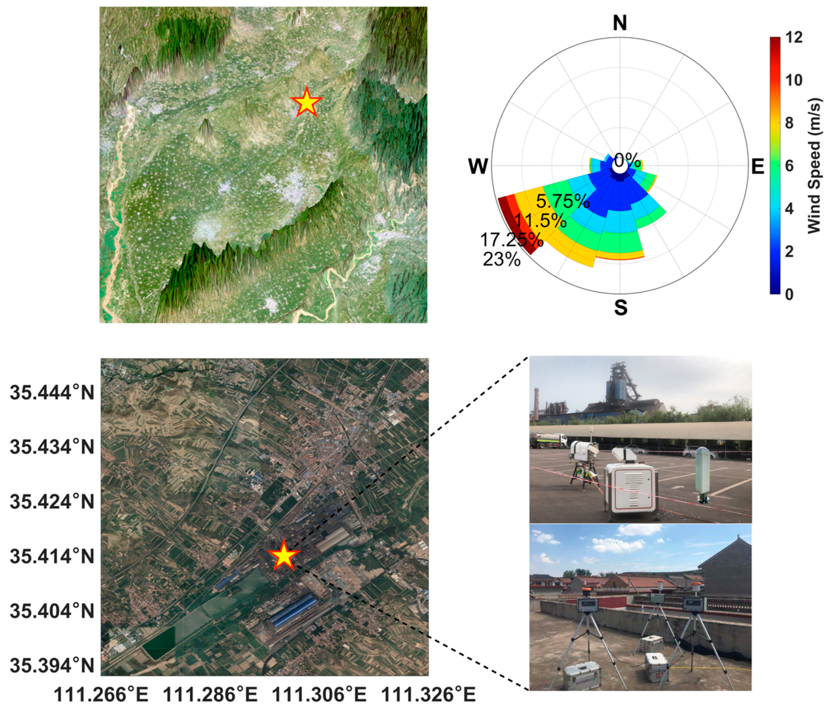
2.1. Observation Site

The steel plant under study is located in the suburb of Wenxi County, Yuncheng City, Shanxi Province, China, and the detailed geographic information of its surrounding area is shown in Figure 1. No large anthropogenic emission sources are located within 50 km of the steel plant, suggesting that it is the main local anthropogenic emission source. There are a few residential areas and two highways or railroad lines around the steel plant, and the rest of the area is almost all bare ground. The plant produces 5.6 million tons of iron, and 8.6 million tons of steel and steel products annually. In 2020, the organized annual emissions of SO₂ were 672 tons, NO_x amounted to 1397 tons, and particulate matters were 417 tons. The sintering (high-temperature metallurgical process) area of the steel plant totaled 825 m², and the volume of the elevated emission source totaled 5400 m³, indicating that the steel plant is a strong single anthropogenic emission source. The high spatial and temporal resolution, high-precision remote sensing instrumentation observation set is located inside the steel plant to enable better access to the boundary layer structure over the strong anthropogenic source emissions. The observation period was from 21 May to 21 June 2021.

2.2. Instrumentations

2.2.1. Microwave Radiometer

The microwave radiometer (RPG-HATPRO-G5, Meckenheim, Germany) is a passive microwave remote sensing device capable of acquiring real-time and continuous information on atmospheric temperature and humidity in the atmosphere over a vertical range of 0–10 km [5,26]. The RPG-HATPRO-G5 acquires vertical atmospheric temperature and humidity information primarily through remote sensing including seven frequency channels for water vapor absorption lines and seven frequency channels for oxygen absorption lines. Based on spectral theory, spectral line correlation, and empirical validation, the optimal number of channels and independent bandwidths within the typical atmospheric microwave water vapor and oxygen windows are selected. And, a highly stable multi-channel parallel filter receiver set system is also utilized to detect the bright temperature. Finally, information on temperature, humidity, liquid water, and water vapor content in the 0–10 km altitude range is obtained by using forward simulated microwave radiation from local multi-year sounding data, infrared instrumentation, ground-based miniature weather stations, neural networks, and regression algorithms. The instrument supports two different scanning modes—the zenith mode and the boundary layer multi-angle scanning mode—and the combined use of the two modes can realize the detection of the whole troposphere (50–250 m vertical resolution up to 10,000 m) and the boundary layer (<1200 m, 30–40 m vertical resolution). Observations up to 93 layers in the vertical direction greatly improve the vertical resolution of the profile while ensuring high accuracy. The vertical resolution of the profile is 10–30 m from the ground to 0.5 km, 40–90 m from 0.5 km to 2.5 km, and 100–200 m from 2 km to 10 km, with a time resolution of 1 s. For more details, refer to http://www.radiometer-physics.de (accessed on 1 September 2023). The detection results of the RPG-HATPRO-G5 have high accuracy and basically do not need further data quality control. Zhao et al. [27] compared the detection results of this microwave radiometer with the routine observation of the 325 m meteorological tower in Beijing, and the results showed that the temperature and humidity detection results of the microwave radiometer and the observation results of the meteorological tower have a very consistent trend, with correlation coefficients of about 0.95. The deviation of the temperature is less than 1 degree, and the deviation of the relative humidity is less than 6%.

2.2.2. Doppler Wind Lidar

Vertical wind speed and horizontal wind vector profiles were obtained using a Doppler wind lidar (Windcube 100s, Leosphere, Paris, France), a Doppler long-range wind lidar manufactured by Leosphere, France, which is an active remote sensing device based on light detection and ranging techniques [28]. The Doppler wind lidar laser emits laser pulses into the atmosphere, which are backscattered and Doppler shifted when they encounter moving suspended particles (dust and water droplets in clouds and fog, polluted aerosols, salt crystals, and biomass burning aerosols). The size of this shift is proportional to the radial wind speed of the particulate matter. Lidar collects the scattered backward echo signals and uses a specific signal processing algorithm to determine the Doppler shift of the backscattered signals. By analyzing the frequency shift in the backscattered echo signal, the radial wind speed and direction along the receiving path can be calculated. The wind lidar runs in Doppler Beam Swinging (DBS) mode, and the cone scanning is done upward at an angle (15° or 30°) and measures the radial wind speed in four directions (east, south, west, and north). Combined with the scanning cone angle and trigonometric relationships, the horizontal wind speed (including the u, v component), wind direction, and vertical wind speed can be obtained. The radial wind speed range is from −30 m·s⁻¹ to 30 m·s⁻¹, and the azimuth range is from 0 to 360°. The detection blind zone is the range from the ground to 50 m altitude above, and the detection range is from 50 m to about 3 km altitude. The wind profile has a temporal resolution of 5 s, a vertical spatial resolution of 25 m, and a wind speed accuracy of 0.5 m·s⁻¹. This Doppler laser wind lidar uses the Carrier to Noise Ratio (CNR) for quality control of data, and data with a CNR of less than −30 dBZ are generally discarded. The results of Dai et al. [29] show that the horizontal wind speed measurements of this wind lidar match very well with the horizontal wind speed measurements of the 325 m meteorological tower in Beijing, with high correlation coefficients R of 0.80–0.97. For more details, refer to www.leosphere.com. Due to the influence of the attenuation of the laser detection power of the wind lidar in the upper atmosphere, the local atmospheric aerosol distribution, and the strong transient change of the wind field, the calculated Doppler shift of the wind lidar’s echo signal in the upper atmosphere cannot meet the CNR requirement of the data quality control, and therefore the data of this part of the air layer are ignored. Data not detected by wind radar in this study (basically, above 1.5 km) are supplemented by the fifth generation of global atmospheric reanalysis data (ERA5) from the European Centre for Medium-Range Weather Forecasts (ECMWF).

2.2.3. CL51 Ceilometer

The ceilometer lidar is a major active remote sensing device used to determine the altitude of the cloud base and to collect the atmospheric backscatter coefficient in the vertical direction, and it has been widely used in boundary layer detection studies in recent years [30,31]. In this paper, a ceilometer lidar (CL51, Vaisala, Vantaa, Finland) is used to acquire backscatter coefficient and BLH data. The backwards scattering caused by haze, fog, precipitation, and clouds is measured as the laser pulse passes through the sky and processed to produce the backscatter coefficient. Due to the particle scattering effect, the actual return signal received by the ceilometer lidar reflects information about the backwards scattering characteristics of the atmosphere at a certain altitude. The height of the cloud base can be calculated from the time difference between the emission of the laser pulse and the reception of the backwards scattering signal. Thus, the CL51 provides atmospheric backwards scattering information from the ground to an altitude of 10–15,000 m with a spatial resolution of 10 m and a time resolution of 15–16 s. For more details, refer to https://www.vaisala.com/en/products/weather-environmental-sensors/ceilometer-CL31-C51-general-info (accessed on 1 September 2023). The data from the CL51 were smoothed, corrected, and quality controlled by the Boundary Layer View software (BL-View, version: 1.0.0) developed by Vaisala, Inc., and the boundary layer heights with three levels of quality confidence were output. The highest confidence level boundary layer height was used in this study.

2.3. Methodology

2.3.1. Temperature Inversion

$$\mathrm{Temp}. \mathrm{Gradient}=\frac{\Delta T}{\Delta Z }\times 100$$

(1)

where T is the temperature (K), and Z is the height (m). Temp. Gradient denotes the inversion intensity in temperature (K/100 m). A positive value of Temp. Gradient represents the occurrence of a temperature inversion. The larger the value is, the more stable the atmosphere is. The negative value one generally indicates an unstable stratification. Similarly, the larger the absolute value is, the more unstable the atmosphere is. Under the special condition of the Temp. Gradient being equal to or around 0, the atmosphere is neutral [6,7].

2.3.2. Turbulent Kinetic Energy (TKE)

The hourly TKE profile is retrieved from the u, v, and w observed by the Doppler wind measurement lidar by the following equation:

$$\mathrm{TKE}=0.5\times \left({\delta }_u^2+{\delta }_v^2+{\delta }_w^2\right)$$

(2)

where ${\delta }_w^2$, ${\delta }_u^2$, and ${\delta }_v^2$ refer to the standard deviation of the instantaneous observed vertical wind speed and horizontal wind speed components in the latitudinal and longitudinal directions in each hour, respectively. The three variables are calculated through the following equations:

$${\delta }_u^2=\frac{1}{N-1}{{\displaystyle \sum }}_{i=1}^N{(u_i-\overline{u})}^2$$

(3)

$${\delta }_v^2=\frac{1}{N-1}{{\displaystyle \sum }}_{i=1}^N{(v_i-\overline{v})}^2$$

(4)

$${\delta }_w^2=\frac{1}{N-1}{{\displaystyle \sum }}_{i=1}^N{(w_i-\overline{w})}^2$$

(5)

where, N represents the number of instantaneous winds collected per hour, $w_i$ and $u_i$($v_i$) represent the i_th vertical wind speed (m/s), and the i_th horizontal wind components in the latitudinal (longitudinal) direction (m/s). $\overline{w}$ and $\overline{u }$($\overline{v }$) represent the average vertical wind speed and the horizontal wind components in the latitudinal (longitudinal) direction in each hour (m/s) [6,32,33].

2.3.3. Gradient Richard Number

$$Ri=\frac{g}{{\theta }_v}\frac{\frac{\partial {\theta }_v}{\partial z}}{{\left(\frac{\partial u}{\partial z}\right)}^2+{\left(\frac{\partial v}{\partial z}\right)}^2}$$

(6)

where θ_v is the virtual potential temperature, and g is the acceleration of gravity, i.e., 9.8 m/s². Previous studies have demonstrated that the laminar flow becomes unstable when Ri is smaller than the critical value of 0.25 [1,34]. Therefore, we adopt the value of 0.25 as a criterion to determine whether a layer of turbulence is stable or not and determine the height of the boundary layer (Ri-BLH) based on this threshold value.

2.3.4. Ventilation Coefficient

The ventilation coefficient (V_H, unit: m²/s), representing the diffusion conditions within the height of the BLH, can be estimated by the following equation:

$$V_H={{\displaystyle \sum }}_{i=1}^n{U}_i\left(Z_i\right)·\Delta Z_i$$

(7)

where, n denotes the number of detectable layers within the BLH detected by the remote sensing equipment, U_i(Z_i) is the horizontal wind velocity (m·s⁻¹) at i level, and ∆Z_i is the height (m) at i level [35]. In this study, the BLH is derived from radar observation. Meanwhile, this paper slightly changes the ventilation coefficient by changing the BLH in the formula into all the observed altitudes in the wind profile radar and obtains the ‘ventilation coefficient’ at different altitudes, which is called “atmospheric diffusion capacity”, to explore the diffusion conditions at different altitudes.

2.3.5. Calculations of Different Types of BLH

From the point of view of thermal interaction, the height at which the temperature gradient is clearly discontinuous or the daily variation of temperature is close to disappearing can be considered as the BLH (Thermal-BLH) [14,15]. During the day, the height of the mixed layer or the location of the top of the inversion are usually considered as the top of the convective boundary layer. At night, the height of the inversion layer or grounded inversion layer is defined as the stable boundary layer height. From the point of view of turbulence motion, the BLH is the thickness of the lowest air layer where turbulence persists, and the height where turbulence energy or turbulence stress is close to disappearing can be regarded as the top of the boundary layer [16]. In this paper, the Richardson number is used for determination. When the Richardson number exceeds the critical Richardson number (Ri_c, 0.25) or the Richardson number gradient changes significantly, it is determined as the turbulence active height, i.e., the BLH (Ri-BLH). From the material distribution point of view, the spatial distribution of aerosols is used to determine the BLH. The aerosol concentration within the BLH is high, so the height where the aerosol concentration gradient is obviously discontinuous is taken as the BLH (Material-BLH) [14,15,17,18]. In this paper, the backscatter coefficient of the CL51 ceilometer is used as the basis for determining the Material-BLH.

3. Results

3.1. Variation of Different Types of Boundary Layer Structures

3.1.1. Thermal Boundary Layer

Figure 2 shows the observational thermal structure of the temperature gradient and relative humidity at the steel plant. In general, the near-surface atmosphere of the steel plant is found to be frequently accompanied by the frequent appearance of temperature inversions at night. Sometimes, these temperature inversions can even reach the grounded surface, indicating a strong stability of the local nighttime boundary layer atmosphere. This may be related to the large amount of heat emitted from the plant’s elevated sources. The stable boundary layer height at night ranged from 50 m to 450 m. And, the Thermal-BLH during the daytime was more stable in values, which was often around 700–800 m. Regarding the humidity condition, it was noticed that as the season moved into the hot summer, the water vapor content in the local atmosphere increased accordingly. In addition, excluding moments of cloud and precipitation (e.g., 23 May, 31 May, 2 June, 9 June, and 14 to 18 June), water vapor was mainly concentrated within the boundary layer and presented a clear line of demarcation in the upper atmosphere.

3.1.2. Dynamic Boundary Layer

The horizontal and vertical wind field structure and TKE variations during the observation period are shown in Figure 3. It was discovered that the presence of significant temperature inversions at night matched the static or small wind speed conditions, which were usually smaller than 2–3 m/s, whereas, when the wind speed increased at night, the temperature inversions almost disappeared (e.g., 28 May, 31 May, 8 June, 9 June, etc.), indicating the effective diffusion ability of wind speed on the local atmosphere. Since the steel plant was located in a huge “canyon” along a southwest–northeast direction (Figure 1), the southwesterly wind appeared frequently during most of the daytime affected by the topography. At night, the emissivity of surface longwave radiation cooled the near-surface layer, and the daytime southwesterly winds gradually weakened. The low mountain winds from the eastern and northeastern hillsides therewith began to dominate, but the mountain wind speed was usually low, providing favorable conditions for the formation of local temperature inversions. Nevertheless, above the height of 300–500 m, the mountain winds gradually weakened, and the wind field remained dominated by topography-induced southwesterly winds. At the same time, the weaker vertical wind speed at night reduced the vertical diffusion of heat and provided good stabilization conditions for the accumulation of heat emitted by the steel plant source. The TKE during the observation period was generally compatible with the wind field. When the wind speed was higher, the resulting mechanical turbulence was stronger and the TKE was therefore larger. Both the TKE (Figure 3c) and Richardson number (Figure 5a) are indicators of the active degree of turbulence. According to the TKE, Richardson number and Ri-BLH (Figure 5a), the turbulent effect within the advective layer was also more active at night. After sunrise, with the gradual enhancement of solar radiation energy, the turbulent height increased accordingly, and the variations of Ri-BLH and T-BLH were highly consistent.

During the period when the local dominant wind direction was typical southwest wind, its wind field exhibited obvious daily variation characteristics, and the relevant results are shown in Figure 4 (daily variation of wind rose plots at different heights). After 8:00 (around sunrise), with the enhancement of the solar radiation and forced by the large-scale meteorological field and the complex surface, the winds at the steel plant were mainly a uniform southwesterly airflow in the valley and remained consistent in the lower atmosphere. After 20:00 (around sunset), affected by the topography and the surface, the radiative cooling of the hillside of the eastern mountain range was faster than that of the place at the same altitude, and a small easterly wind flow (with a wind speed of less than 2 m/s) started to appear locally, which strengthened during the night and gradually took the dominant position; its frequency of occurrence in the lower layer can be up to ~80%. While the probability of occurrence of the southwesterly winds was significantly reduced compared with that during the daytime, and it could decrease from ~100% during the daytime to ~20%. In addition, this low-speed easterly wind flow could develop to a certain height, which was obvious in the height range of 100 m and weaker above 200 m. When the solar radiation increased at sunrise, the easterly wind flow gradually disappeared again, and the southwesterly wind flow prevailed. This kind of local wind direction and speed transformation with obvious daily changes also showed the local atmospheric diffusion ability under typical weather conditions to a certain extent. Under the background of relatively stable large-scale circulation, the wind speed was a little bit larger during the daytime, and the wind direction was almost uniform in the lower layer and evenly distributed throughout the atmosphere, which could diffuse the pollutants better. But, the southwesterly wind was weakened significantly at night (especially in the low altitude range of 50 m), and there was a clear easterly low-speed airflow or even a northeasterly airflow in the altitude range of 100 m. At 100 m, there was an obvious easterly low-speed airflow, or even a northeasterly airflow, which could blow the pollutants back to the local area during the daytime. However, above the 100 m altitude range, this daily variation disappeared, and the wind speed was higher, indicating that the pollutants could be effectively dispersed at this altitude.

3.1.3. Material Boundary Layer

Figure 5b shows the structure and height of the material boundary layer over the steel plant. The ceilometer uses the detected backscatter coefficient profile in the vertical direction to determine the vertical aerosol distribution, and therefore, it can be used to study the aerosol distributions across the boundary layer and determine the Material-BLH [17,18,36]. By excluding the increase in the high backscatter coefficient during times of precipitation from 14 to 18, June, the 100–200 m BLH at night further inhibited the atmospheric diffusion capacity, causing the steel plant to discharge heat along with pollutants into the near-surface atmosphere, resulting in a larger backscatter coefficient in the near-surface layer at night. In addition, the Material-BLH at night matched well with the Thermal-BLH, and more pollutants accumulated above the steel plant while temperature inversions formed.

Figure 5. Richardson number (a) and backscatter coefficient (b) boundary layer structure of Jianlong Steel Plant during the observation period of 21 May to 21 June 2021 (arrows: horizontal wind).

Figure 5. Richardson number (a) and backscatter coefficient (b) boundary layer structure of Jianlong Steel Plant during the observation period of 21 May to 21 June 2021 (arrows: horizontal wind).

3.2. Ventilation Coefficient

Figure 6 shows the variation of atmospheric diffusion capacity and the ventilation coefficient above the steel plant. Generally, the ventilation coefficient during the haze events tends to be less than 2000–3000 m²·s⁻¹ or even less than 500–1000 m²·s⁻¹ [35]. It was found that the zone of higher atmospheric diffusion capacity (i.e., greater than 4000 to 5000 m²·s⁻¹) during the daytime could drop down to about 250–500 m, while the region of weaker atmospheric diffusion capacity (less than 4000 m²·s⁻¹) during the nighttime could rise up to about 1000 m at the highest, which indicated the differences between daytime and nighttime atmospheric diffusion capacity. Figure 6b shows the pronounced daily variation characteristics of atmospheric diffusion capacity and the ventilation coefficient. The wind speed was higher during the daytime and accompanied by uniform wind direction, leading to an excellent ventilation coefficient and atmospheric diffusion capacity. At night, the wind speed was usually lower with a static scenario, so the ventilation coefficient and atmospheric diffusion capacity were worse, especially in the lower level of 50 m. The average atmospheric diffusion capacity and ventilation coefficient were less than 250 m²/s, making it more difficult for pollutants to spread outside and deteriorating the air quality by the strong intensity of the emission source. Therefore, combining the different characteristics of daily changes in local wind direction below or above 100 m, as mentioned above, the emission heights of organized emissions discharging a great number of pollutants can be concentrated to 100 m in the subsequent new construction or renovation measures, so as to make it more efficient for the pollutants to diffuse and reduce their impact on the surrounding area.

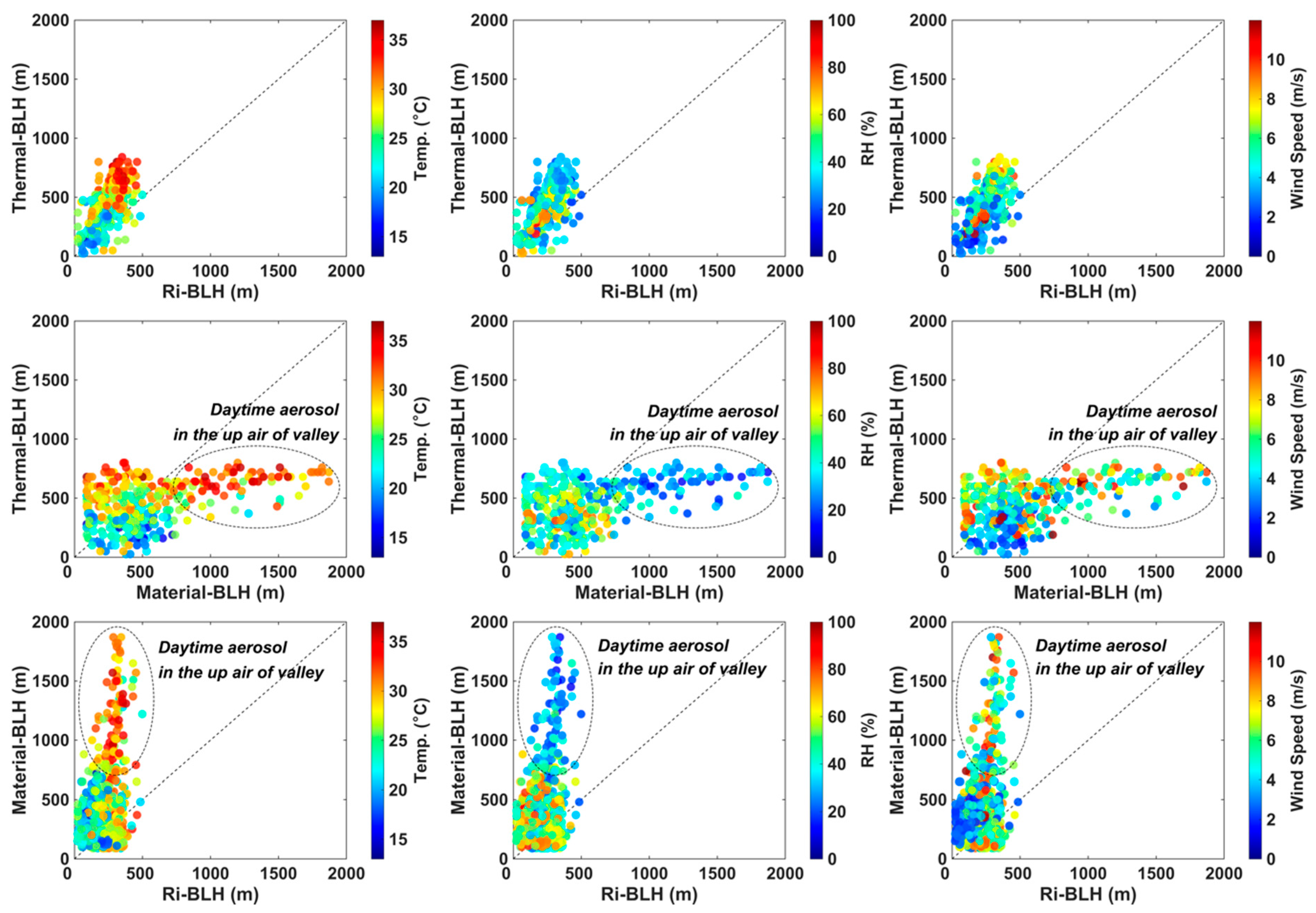
3.3. Inter-Comparison of Thermal-BLH, Ri-BLH, and Material-BLH

The relationships between the three types of BLH are referenced in Figure 7 (cloud and precipitation hours have been removed). It was found that the Thermal-BLH and Ri-BLH were, in general, highly consistent, which was mainly due to the fact that temperature variations were decisive for thermal turbulence. Nevertheless, Thermal-BLH was slightly higher than Ri-BLH, especially at high daytime temperatures and low humidity during a clear daytime. This may be related to the larger uncertainty of Ri_c, which is not a constant but a function of the overall stability of the atmosphere. The detectable rate of the stable boundary layer height is low, and it is tough to accurately identify the convective boundary layer height, as well. Material-BLH maintained a better consistent relationship with both the Thermal-BLH and Ri-BLH in low BLH scenarios. However, with a rise in the BLH, the Material-BLH grew much faster than the Thermal-BLH and Ri-BLH, and the Material-BLH had higher overall height values. Similarly, the higher heights of the Material-BLH than the other two boundary layers were mainly accompanied by higher temperatures, lower humidity, and higher wind speeds, indicating that this phenomenon primarily appeared during the daytime. The vigorous convection tended to lift aerosols from the surface up to the aloft atmosphere, especially when there existed a powerful emission source on the underlying surface, which eventually resulted in a relatively hazy scenario. This was also supported by the intraday variations of the three BLH (Figure 8). The trends of the three BLH were consistent. The Ri-BLH was lower than the other two types of BLH, and there was a large underestimation especially during the daytime. The Thermal-BLH and Material-BLH were basically the same at night, and the Material-BLH was slightly higher during the daytime, which was related to the previously mentioned daytime convectively uplifted aerosol and the aerosol at the top of the valley. As a result, the Material-BLH was often significantly higher than the Thermal-BLH and Ri-BLH during the daytime, but as can be seen from Figure 5b, the regions with a strong backscatter coefficient (i.e., regions of aerosol concentration) were still concentrated at heights below the Thermal-BLH and Ri-BLH.

4. Conclusions and Outlooks

Through one month of monitoring the thermodynamics of the summertime boundary layer in high temporal and vertically spatial resolutions over a typical steel plant in Shanxi province, middle China, the boundary layer structures were systematically explored:

(1) Strong nighttime temperature inversions or grounded temperature inversions were evidenced to frequently occur above the steel industry, which made it easier to constrain the pollutants within the grounding layer by cooperating with the severe pollutant emissions. The local wind field showed a certain pattern of daily change in the typical large-scale circulation background, which was mainly reflected in the fact that the airflow in the whole layer was dominated by a southwesterly wind during the daytime, the wind direction was uniform, the wind speed was a little bit larger, and the atmospheric diffusion capacity was strong. At night, due to the weakening of solar radiation, topography, and the influence of the surface, the easterly low-speed airflow was the dominant airflow within 100 m in the low altitude range, and the atmospheric diffusion capacity was weak, while the upper level was still dominated by the southwest wind.

(2) Vertical detection showed that for every 50 m rise in vertical height, the average ventilation coefficient could be increased by about 2~3 times, and pollutants could be rapidly diffused at a height of 100 m. In view of the rapid development of the current atmospheric boundary layer detection technology and air pollution monitoring technology, the systematic construction of air pollution monitoring and vertical diffusion capacity detection and evaluation systems for the target area could provide more scientific guidance for the strong pollutant-emitting enterprises and industrial zones to accurately manage air pollutant emissions and environmental safety protection.

(3) The three different definitions of BLH (i.e., thermal, dynamic, and material BLH) revealed that the local BLH at the steel plant ranged from 600 to 1500 m during the daytime and became lower than 200–300 m at night. The heights for the thermal and dynamic boundary layers were highly similar; nevertheless, the height of the material boundary layer was significantly higher than the other two types because of the strong convections. Even so, the majority of aerosols were still constrained below the heights of the thermal and dynamic boundary layers. For the sake of accurately assessing the local atmospheric dispersion capacity and developing scientific and feasible pollutant emission planning for steel plants, numerical simulation focusing on small local regions is a promising tool to explicitly track the transport path of air pollutants, which could provide scientific and technical references for the air quality managements of steel plants.

References

1. Stull, R.B. An Introduction to Boundary Layer Meteorology; Springer: Dordrecht, The Netherlands, 1988. [Google Scholar]
2. Jiang, Y.; Xin, J.; Wang, Z.; Tian, Y.; Tang, G.; Ren, Y.; Wu, L.; Pan, X.; Wang, Y.; Jia, D.; et al. The dynamic multi-box algorithm of atmospheric environmental capacity. Sci. Total Environ. 2022, 806, 150951. [Google Scholar] [CrossRef]
3. Yang, Y.; Fan, S.; Wang, L.; Gao, Z.; Zhang, Y.; Zou, H.; Miao, S.; Li, Y.; Huang, M.; Yim, S.H.L.; et al. Diurnal Evolution of the Wintertime Boundary Layer in Urban Beijing, China: Insights from Doppler Lidar and a 325-m Meteorological Tower. Remote Sens. 2020, 12, 3935. [Google Scholar] [CrossRef]
4. Yang, Y.; Guo, M.; Ren, G.; Liu, S.; Zong, L.; Zhang, Y.; Zheng, Z.; Miao, Y.; Zhang, Y. Modulation of Wintertime Canopy Urban Heat Island (CUHI) Intensity in Beijing by Synoptic Weather Pattern in Planetary Boundary Layer. J. Geophys. Res. Atmos. 2022, 127, e2021JD035988. [Google Scholar] [CrossRef]
5. Zhang, L.; Xin, J.; Yin, Y.; Chang, W.; Xue, M.; Jia, D.; Ma, Y. Understanding the Major Impact of Planetary Boundary Layer Schemes on Simulation of Vertical Wind Structure. Atmosphere 2021, 12, 777. [Google Scholar] [CrossRef]
6. Zhao, D.; Liu, G.; Xin, J.; Quan, J.; Wang, Y.; Wang, X.; Dai, L.; Gao, W.; Tang, G.; Hu, B.; et al. Haze pollution under a high atmospheric oxidization capacity in summer in Beijing: Insights into formation mechanism of atmospheric physicochemical processes. Atmos. Chem. Phys. 2020, 20, 4575–4592. [Google Scholar] [CrossRef]
7. Zhao, D.; Xin, J.; Gong, C.; Quan, J.; Wang, Y.; Tang, G.; Ma, Y.; Dai, L.; Wu, X.; Liu, G.; et al. The impact threshold of the aerosol radiative forcing on the boundary layer structure in the pollution region. Atmos. Chem. Phys. 2021, 21, 5739–5753. [Google Scholar] [CrossRef]
8. Ma, Y.; Ye, J.; Xin, J.; Zhang, W.; Vilà-Guerau de Arellano, J.; Wang, S.; Zhao, D.; Dai, L.; Ma, Y.; Wu, X.; et al. The Stove, Dome, and Umbrella Effects of Atmospheric Aerosol on the Development of the Planetary Boundary Layer in Hazy Regions. Geophys. Res. Lett. 2020, 47, e2020GL087373. [Google Scholar] [CrossRef]
9. Ma, Y.; Tian, Y.; Ren, Y.; Wang, Z.; Wu, L.; Pan, X.; Ma, Y.; Xin, J. Long-Term (2017–2020) Aerosol Optical Depth Observations in Hohhot City in Mongolian Plateau and the Impacts from Different Types of Aerosol. Atmosphere 2022, 13, 737. [Google Scholar] [CrossRef]
10. Xin, J.; Ma, Y.; Zhao, D.; Gong, C.; Ren, X.; Tang, G.; Xia, X.; Wang, Z.; Cao, J.; de Arellano, J.V.-G.; et al. The feedback effects of aerosols from different sources on the urban boundary layer in Beijing China. Environ. Pollut. 2023, 325, 121440. [Google Scholar] [CrossRef] [PubMed]
11. Wang, L.; Stanič, S.; Bergant, K.; Eichinger, W.; Močnik, G.; Drinovec, L.; Vaupotič, J.; Miler, M.; Gosar, M.; Gregorič, A. Retrieval of Vertical Mass Concentration Distributions—Vipava Valley Case Study. Remote Sens. 2019, 11, 106. [Google Scholar] [CrossRef]
12. Wang, L.; Stanič, S.; Eichinger, W.; Song, X.; Zavrtanik, M. Development of an Automatic Polarization Raman LiDAR for Aerosol Monitoring over Complex Terrain. Sensors 2019, 19, 3186. [Google Scholar] [CrossRef]
13. Wang, L.; Yin, Z.; Bu, Z.; Wang, A.; Mao, S.; Yi, Y.; Müller, D.; Chen, Y.; Wang, X. Quality assessment of aerosol lidars at 1064nm in the framework of the MEMO campaign. Atmos. Meas. Tech. 2023, 16, 4307–4318. [Google Scholar] [CrossRef]
14. Moreira, G.d.A.; Guerrero-Rascado, J.L.; Bravo-Aranda, J.A.; Foyo-Moreno, I.; Cazorla, A.; Alados, I.; Lyamani, H.; Landulfo, E.; Alados-Arboledas, L. Study of the planetary boundary layer height in an urban environment using a combination of microwave radiometer and ceilometer. Atmos. Res. 2020, 240, 104932. [Google Scholar] [CrossRef]
15. Jiang, Y.; Xin, J.; Wang, Y.; Tang, G.; Zhao, Y.; Jia, D.; Zhao, D.; Wang, M.; Dai, L.; Wang, L.; et al. The thermodynamic structures of the planetary boundary layer dominated by synoptic circulations and the regular effect on air pollution in Beijing. Atmos. Chem. Phys. 2021, 21, 6111–6128. [Google Scholar] [CrossRef]
16. Dai, C.; Wang, Q.; Kalogiros, J.A.; Lenschow, D.H.; Gao, Z.; Zhou, M. Determining Boundary-Layer Height from Aircraft Measurements. Bound.-Layer Meteorol. 2014, 152, 277–302. [Google Scholar] [CrossRef]
17. Münkel, C.; Eresmaa, N.; Räsänen, J.; Karppinen, A. Retrieval of mixing height and dust concentration with lidar ceilometer. Bound.-Layer Meteorol. 2007, 124, 117–128. [Google Scholar] [CrossRef]
18. Emeis, S.; Schäfer, K. Remote Sensing Methods to Investigate Boundary-layer Structures relevant to Air Pollution in Cities. Bound.-Layer Meteorol. 2006, 121, 377–385. [Google Scholar] [CrossRef]
19. Tompkins, A.M. A Prognostic Parameterization for the Subgrid-Scale Variability of Water Vapor and Clouds in Large-Scale Models and Its Use to Diagnose Cloud Cover. J. Atmos. Sci. 2002, 59, 1917–1942. [Google Scholar] [CrossRef]
20. Liu, G.; Xin, J.; Wang, X.; Si, R.; Ma, Y.; Wen, T.; Zhao, L.; Zhao, D.; Wang, Y.; Gao, W. Impact of the coal banning zone on visibility in the Beijing-Tianjin-Hebei region. Sci. Total Environ. 2019, 692, 402–410. [Google Scholar] [CrossRef] [PubMed]
21. Zhao, D.; Xin, J.; Wang, W.; Jia, D.; Wang, Z.; Xiao, H.; Liu, C.; Zhou, J.; Tong, L.; Ma, Y.; et al. Effects of the sea-land breeze on coastal ozone pollution in the Yangtze River Delta, China. Sci. Total Environ. 2022, 807, 150306. [Google Scholar] [CrossRef] [PubMed]
22. Liu, B.; Ma, X.; Ma, Y.; Li, H.; Jin, S.; Fan, R.; Gong, W. The relationship between atmospheric boundary layer and temperature inversion layer and their aerosol capture capabilities. Atmos. Res. 2022, 271, 106121. [Google Scholar] [CrossRef]
23. Tian, P.F.; Cao, X.J.; Zhang, L.; Sun, N.X.; Sun, L.; Logan, T.; Shi, J.S.; Wang, Y.; Ji, Y.M.; Lin, Y.; et al. Aerosol vertical distribution and optical properties over China from long-term satellite and ground-based remote sensing. Atmos. Chem. Phys. 2017, 17, 2509–2523. [Google Scholar] [CrossRef]
24. Tian, P.F.; Zhang, L.; Ma, J.M.; Tang, K.; Xu, L.L.; Wang, Y.; Cao, X.J.; Liang, J.N.; Ji, Y.M.; Jiang, J.H.; et al. Radiative absorption enhancement of dust mixed with anthropogenic pollution over East Asia. Atmos. Chem. Phys. 2018, 18, 7815–7825. [Google Scholar] [CrossRef]
25. Tian, P.F.; Yu, Z.R.; Cui, C.; Huang, J.P.; Kang, C.L.; Shi, J.S.; Cao, X.J.; Zhang, L. Atmospheric aerosol size distribution impacts radiative effects over the Himalayas via modulating aerosol single-scattering albedo. NPJ Clim. Atmos. Sci. 2023, 6, 54. [Google Scholar] [CrossRef]
26. Ahn, M.H.; Won, H.Y.; Han, D.; Kim, Y.H.; Ha, J.C. Characterization of downwelling radiance measured from a ground-based microwave radiometer using numerical weather prediction model data. Atmos. Meas. Tech. 2016, 9, 281–293. [Google Scholar] [CrossRef]
27. Zhao, D.; Xin, J.; Gong, C.; Quan, J.; Liu, G.; Zhao, W.; Wang, Y.; Liu, Z.; Song, T. The formation mechanism of air pollution episodes in Beijing city: Insights into the measured feedback between aerosol radiative forcing and the atmospheric boundary layer stability. Sci. Total Environ. 2019, 692, 371–381. [Google Scholar] [CrossRef]
28. Canadillas, B.A.; Bégué, A.; Neumann, T. Comparison of turbulence spectra derived from LiDAR and sonic measurements at the offshore platform FINO1. In Proceedings of the 10th German Wind Energy Conference 2010, Bremen, Germany, 17–18 November 2010. [Google Scholar]
29. Dai, L.; Xin, J.; Zuo, H.; Ma, Y.; Zhang, L.; Wu, X.; Ma, Y.; Jia, D.; Wu, F. Multilevel Validation of Doppler Wind Lidar by the 325 m Meteorological Tower in the Planetary Boundary Layer of Beijing. Atmosphere 2020, 11, 1051. [Google Scholar] [CrossRef]
30. Tang, G.; Zhu, X.; Hu, B.; Xin, J.; Wang, L.; Münkel, C.; Mao, G.; Wang, Y. Impact of emission controls on air quality in Beijing during APEC 2014: Lidar ceilometer observations. Atmos. Chem. Phys. 2015, 15, 12667–12680. [Google Scholar] [CrossRef]
31. Tang, G.; Zhang, J.; Zhu, X.; Song, T.; Münkel, C.; Hu, B.; Schäfer, K.; Liu, Z.; Zhang, J.; Wang, L.; et al. Mixing layer height and its implications for air pollution over Beijing, China. Atmos. Chem. Phys. 2016, 16, 2459–2475. [Google Scholar] [CrossRef]
32. Banta, R.M.; Pichugina, Y.L.; Brewer, W.A. Turbulent Velocity-Variance Profiles in the Stable Boundary Layer Generated by a Nocturnal Low-Level Jet. J. Atmos. Sci. 2006, 63, 2700–2719. [Google Scholar] [CrossRef]
33. Wang, L.; Liu, J.; Gao, Z.; Li, Y.; Huang, M.; Fan, S.; Zhang, X.; Yang, Y.; Miao, S.; Zou, H.; et al. Vertical observations of the atmospheric boundary layer structure over Beijing urban area during air pollution episodes. Atmos. Chem. Phys. 2019, 19, 6949–6967. [Google Scholar] [CrossRef]
34. Banakh, V.A.; Smalikho, I.N.; Falits, A.V. Wind–Temperature Regime and Wind Turbulence in a Stable Boundary Layer of the Atmosphere: Case Study. Remote Sens. 2020, 12, 955. [Google Scholar] [CrossRef]
35. Zhang, B. A Simulation Study on the Structure of the Urban Boundary Layer and the Diffusion of SO2 Pollutants over Shenyang; Peking University: Beijing, China, 2011; pp. 92–97. [Google Scholar]
36. Zhu, X.; Tang, G.; Lv, F.; Hu, B.; Cheng, M.; Münkel, C.; Schäfer, K.; Xin, J.; An, X.; Wang, G.; et al. The spatial representativeness of mixing layer height observations in the North China Plain. Atmos. Res. 2018, 209, 204–211. [Google Scholar] [CrossRef]
Figure 1. Location of Jianlong Steel Plant and observation sites (star); and wind rose plot in hourly data during observation period.
Remotesensing 15 05104 g001
Figure 2. Temperature gradient (Temp. Gradient) (a) and relative humidity (RH) (b) boundary layer structure of Jianlong Steel Plant during the observation period of 21 May to 21 June 2021.
Remotesensing 15 05104 g002
Figure 3. Horizontal wind speed (a), vertical wind speed (b), and turbulent kinetic energy (TKE) (c) boundary layer structure of Jianlong Steel Plant during the observation period of 21 May to 21 June 2021 (arrows: horizontal wind).
Remotesensing 15 05104 g003
Figure 4. Diurnal variation characteristics of wind profile of Jianlong Steel Plant during the observation period of 21 May to 21 June 2021.
Remotesensing 15 05104 g004aRemotesensing 15 05104 g004b
Figure 6. Atmospheric diffusion capacity structure (a) and diurnal changes of atmospheric diffusion capacity (b) of Jianlong Steel Plant during the observation period of 21 May to 21 June 2021 (arrows: horizontal wind).
Remotesensing 15 05104 g006
Figure 7. Comparison of Thermal Boundary Layer Height (Thermal-BLH), Richardson Number-Boundary Layer Height (Ri-BLH), and Material Boundary Layer Height (Material-BLH).
Remotesensing 15 05104 g007
Figure 8. Diurnal variations of the boundary layer structure (Temp. Gradient, Thermal-BLH, Ri-BLH, and Material-BLH).
Remotesensing 15 05104 g008
Disclaimer/Publisher’s Note: The statements, opinions and data contained in all publications are solely those of the individual author(s) and contributor(s) and not of MDPI and/or the editor(s). MDPI and/or the editor(s) disclaim responsibility for any injury to people or property resulting from any ideas, methods, instructions or products referred to in the content.