
Mapping of the Spatial Scope and Water Quality of Surface Water Based on the Google Earth Engine Cloud Platform and Landsat Time Series

Abstract
:
1. Introduction
2. Study Area and Datasets
2.1. Study Area
2.2. Datasets
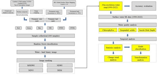
3. Methods
3.1. Data Pre-Processing
3.2. Water Spatial Range Mapping Based on EGS Operational Surface Water Mapping Algorithm
3.3. Accuracy Evaluation of Surface Water Extent Extraction Results
3.4. Inversion and Mapping of Water Quality Parameters
3.5. Analysis of the Spatial Distribution of the Water Bodies and the Evolution of the Temporal-Spatial Patterns of the Water Quality Parameters
4. Results and Analysis
4.1. Spatial Distribution Mapping of Surface Water
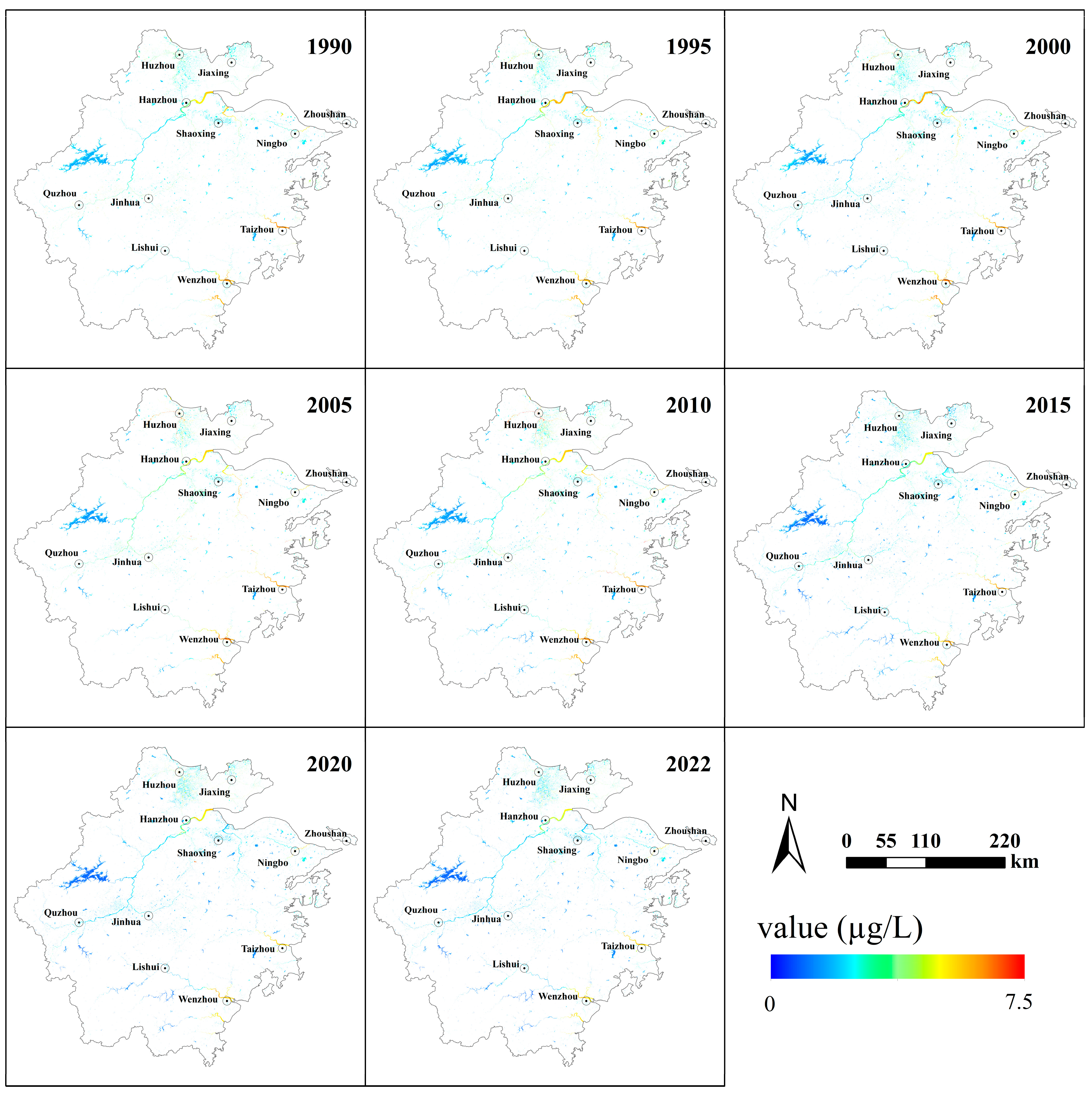
4.2. Inversion of Water Quality Parameters and Water Quality Map
4.2.1. Chlorophyll-a Concentration
4.2.2. Secchi Disk Depth
4.2.3. Suspended Solids Concentration
5. Discussion
5.1. Reliability of Research Results
5.2. Distribution of Surface Water and Water Quality Condition
5.3. Limitations of the Study
6. Conclusions
Author Contributions
Funding
Data Availability Statement
Acknowledgments
Conflicts of Interest
References
- Jia, K.; Jiang, W.; Li, J.; Tang, Z. Spectral Matching Based on Discrete Particle Swarm Optimization: A New Method for Terrestrial Water Body Extraction Using Multi-Temporal Landsat 8 Images. Remote Sens. Environ. 2018, 209, 1–18. [Google Scholar] [CrossRef]
- Sun, G.; Pan, Z.; Zhang, A.; Jia, X.; Ren, J.; Fu, H.; Yan, K. Large kernel spectral and spatial attention networks for hyperspectral image classification. IEEE Trans. Geosci. Remote Sens. 2023, 61, 5519915. [Google Scholar] [CrossRef]
- Fu, H.; Sun, G.; Zhang, L.; Zhang, A.; Ren, J.; Jia, X.; Li, F. Three-dimensional singular spectrum analysis for precise land cover classification from UAV-borne hyperspectral benchmark datasets. ISPRS J. Photogramm. Remote Sens. 2023, 203, 115–134. [Google Scholar] [CrossRef]
- Ten Brinke, W.B.M.; Knoop, J.; Muilwijk, H.; Ligtvoet, W. Social Disruption by Flooding, a European Perspective. Int. J. Disaster Risk Reduct. 2017, 21, 312–322. [Google Scholar] [CrossRef]
- Zhang, Q.; Gu, X.; Shi, P.; Singh, V.P. Impact of Tropical Cyclones on Flood Risk in Southeastern China: Spatial Patterns, Causes and Implications. Glob. Planet. Chang. 2017, 150, 81–93. [Google Scholar] [CrossRef]
- Marton, D.; Kapelan, Z. Risk and Reliability Analysis of Open Reservoir Water Shortages Using Optimization. Procedia Eng. 2014, 89, 1478–1485. [Google Scholar] [CrossRef]
- Jia, M.; Wang, Z.; Mao, D.; Ren, C.; Song, K.; Zhao, C.; Wang, C.; Xiao, X.; Wang, Y. Mapping global distribution of mangrove forests at 10-m resolution. Sci. Bull. 2023, 68, 1306–1316. [Google Scholar] [CrossRef]
- Chen, C.; Wang, L.; Yang, G.; Sun, W.; Song, Y. Mapping of ecological environment based on Google earth engine cloud computing platform and landsat long-term data: A case study of the zhoushan archipelago. Remote Sens. 2023, 15, 4072. [Google Scholar] [CrossRef]
- Mutanga, O.; Kumar, L. Google Earth Engine Applications. Remote Sens. 2019, 11, 591. [Google Scholar] [CrossRef]
- Chen, C.; Liang, J.; Yang, G.; Sun, W. Spatio-temporal distribution of harmful algal blooms and their correlations with marine hydrological elements in offshore areas, China. Ocean. Coast. Manag. 2023, 238, 106554. [Google Scholar] [CrossRef]
- Ding, L.; Wu, H.; Wang, C.J.; Qin, Z.; Zhang, Q. Study of the water body extracting from MODIS images based on spectrum-photometric method. Geomat. Spat. Inf. Technol. 2006, 29, 25–27. [Google Scholar]
- Chen, J.; Chen, S.; Fu, R.; Li, D.; Jiang, H.; Wang, C.; Peng, Y.; Jia, K.; Hicks, B.J. Remote Sensing Big Data for Water Environment Monitoring: Current Status, Challenges, and Future Prospects. Earth’s Future 2022, 10, e2021EF002289. [Google Scholar] [CrossRef]
- McFeeters, S.K. The Use of the Normalized Difference Water Index (NDWI) in the Delineation of Open Water Features. Int. J. Remote Sens. 1996, 17, 1425–1432. [Google Scholar] [CrossRef]
- Xu, H. Modification of Normalised Difference Water Index (NDWI) to Enhance Open Water Features in Remotely Sensed Imagery. Int. J. Remote Sens. 2006, 27, 3025–3033. [Google Scholar] [CrossRef]
- Feyisa, G.L.; Meilby, H.; Fensholt, R.; Proud, S.R. Automated Water Extraction Index: A New Technique for Surface Water Mapping Using Landsat Imagery. Remote Sens. Environ. 2014, 140, 23–35. [Google Scholar] [CrossRef]
- Tulbure, M.G.; Broich, M.; Stehman, S.V.; Kommareddy, A. Surface Water Extent Dynamics from Three Decades of Seasonally Continuous Landsat Time Series at Subcontinental Scale in a Semi-Arid Region. Remote Sens. Environ. 2016, 178, 142–157. [Google Scholar] [CrossRef]
- Wang, G.; Wu, M.; Wei, X.; Song, H. Water Identification from High-Resolution Remote Sensing Images Based on Multidimensional Densely Connected Convolutional Neural Networks. Remote Sens. 2020, 12, 795. [Google Scholar] [CrossRef]
- Li, W.; Zhang, W.; Li, Z.; Wang, Y.; Chen, H.; Gao, H.; Zhou, Z.; Hao, J.; Li, C.; Wu, X. A New Method for Surface Water Extraction Using Multi-Temporal Landsat 8 Images Based on Maximum Entropy Model. Eur. J. Remote Sens. 2022, 55, 303–312. [Google Scholar] [CrossRef]
- Brivio, P.A.; Giardino, C.; Zilioli, E. Determination of Chlorophyll Concentration Changes in Lake Garda Using an Image-Based Radiative Transfer Code for Landsat TM Images. Int. J. Remote Sens. 2001, 22, 487–502. [Google Scholar] [CrossRef]
- Sharaf El Din, E. Enhancing the Accuracy of Retrieving Quantities of Turbidity and Total Suspended Solids Using Landsat-8-Based-Principal Component Analysis Technique. J. Spat. Sci. 2021, 66, 493–512. [Google Scholar] [CrossRef]
- Song, K.; Liu, G.; Wang, Q.; Wen, Z.; Lyu, L.; Du, Y.; Sha, L.; Fang, C. Quantification of Lake Clarity in China Using Landsat OLI Imagery Data. Remote Sens. Environ. 2020, 243, 111800. [Google Scholar] [CrossRef]
- Pekel, J.F.; Cottam, A.; Gorelick, N.; Belward, A.S. High-resolution mapping of global surface water and its long-term changes. Nature 2016, 540, 418–422. [Google Scholar] [CrossRef] [PubMed]
- Peng, J.; Huang, Y.; Sun, W.; Chen, N.; Ning, Y.; Du, Q. Domainadaptation inremote sensing imageclassification: A survey. IEEE J. Sel. Top. Appl. Earth Obs. Remote Sens. 2022, 15, 9842–9859. [Google Scholar] [CrossRef]
- Feng, M.; Sexton, J.O.; Channan, S.; Townshend, J.R. A Global, High-Resolution (30-m) Inland Water Body Dataset for 2000: First Results of a Topographic–Spectral Classification Algorithm. Int. J. Digit. Earth 2016, 9, 113–133. [Google Scholar] [CrossRef]
- Olthof, I.; Rainville, T. Dynamic Surface Water Maps of Canada from 1984 to 2019 Landsat Satellite Imagery. Remote Sens. Environ. 2022, 279, 113121. [Google Scholar] [CrossRef]
- Chen, C.; Chen, Y.; Jin, H.; Chen, L.; Liu, Z.; Sun, H.; Hong, J.; Wang, H.; Fang, S.; Zhang, X. 3D model construction and ecological environment investigation on a regional scale using UAV remote sensing. Intell. Autom. Soft Comput. 2023, 37, 1655–1672. [Google Scholar] [CrossRef]
- Huang, L.; Yu, F.; Zhang, D.; Lin, L. Quantitative Retrieval of Chlorophyll a Concentration Based on Landsat-8 OLI in the Lakes. J. Jiangxi Sci. 2016, 34, 441–456. [Google Scholar]
- Liu, Y.; Zhang, B.; Yao, X.; Zhang, H.; Feng, R. Remote sensing inversion of water transparency in Dongping Lake. J. Surv. Mapp. Sci. 2018, 43, 72–78. [Google Scholar]
- Jie, G.; Yuchun, W.; Jiazhu, H.; Yunmei, L.; Jianguang, W.; Jiangping, G. Suspended Sediment Estimating Models in Lake Taihu Using Remote Sensing Data. J. Lake Sci. 2007, 19, 241–249. [Google Scholar] [CrossRef]
- Yang, H.; Wang, Z.; Zhao, H.; Yu, G. Water Body Extraction Methods Study Based on RS and GIS. Procedia Environ. Sci. 2011, 10, 2619–2624. [Google Scholar]
- Jiang, W.; He, G.; Long, T.; Ni, Y.; Liu, H.; Peng, Y.; Lv, K.; Wang, G. Multilayer Perceptron Neural Network for Surface Water Extraction in Landsat 8 OLI Satellite Images. Remote Sens. 2018, 10, 755. [Google Scholar] [CrossRef]
- Olthof, I. Mapping Seasonal Inundation Frequency (1985–2016) along the St-John River, New Brunswick, Canada Using the Landsat Archive. Remote Sens. 2017, 9, 143. [Google Scholar] [CrossRef]
- Rishikeshan, C.A.; Ramesh, H. An Automated Mathematical Morphology Driven Algorithm for Water Body Extraction from Remotely Sensed Images. ISPRS J. Photogramm. Remote Sens. 2018, 146, 11–21. [Google Scholar] [CrossRef]
- Sheng, Y.; Song, C.; Wang, J.; Lyons, E.A.; Knox, B.R.; Cox, J.S.; Gao, F. Representative Lake Water Extent Mapping at Continental Scales Using Multi-Temporal Landsat-8 Imagery. Remote Sens. Environ. 2016, 185, 129–141. [Google Scholar] [CrossRef]
- Taloor, A.K.; Thakur, P.K.; Jakariya, M. Remote Sensing and GIS Applications in Water Science. Groundw. Sustain. Dev. 2022, 19, 100817. [Google Scholar] [CrossRef]
- Tang, H.; Lu, S.; Ali Baig, M.H.; Li, M.; Fang, C.; Wang, Y. Large-Scale Surface Water Mapping Based on Landsat and Sentinel-1 Images. Water 2022, 14, 1454. [Google Scholar] [CrossRef]
- Wu, G.; De Leeuw, J.; Skidmore, A.K.; Prins, H.H.T.; Liu, Y. Comparison of MODIS and Landsat TM5 Images for Mapping Tempo–Spatial Dynamics of Secchi Disk Depths in Poyang Lake National Nature Reserve, China. Int. J. Remote Sens. 2008, 29, 2183–2198. [Google Scholar] [CrossRef]
- Xing, W.; Guo, B.; Sheng, Y.; Yang, X.; Ji, M.; Xu, Y. Tracing Surface Water Change from 1990 to 2020 in China’s Shandong Province Using Landsat Series Images. Ecol. Indic. 2022, 140, 108993. [Google Scholar] [CrossRef]
- Yang, X.; Qiu, S.; Zhu, Z.; Rittenhouse, C.; Riordan, D.; Cullerton, M. Mapping understory plant communities in deciduous forests from Sentinel-2 time series. Remote Sens. Environ. 2023, 293, 113601. [Google Scholar] [CrossRef]
- Yue, L.; Li, B.; Zhu, S.; Yuan, Q.; Shen, H. A Fully Automatic and High-Accuracy Surface Water Mapping Framework on Google Earth Engine Using Landsat Time-Series. Int. J. Digit. Earth 2023, 16, 210–233. [Google Scholar] [CrossRef]
- Huang, Y.; Peng, J.; Sun, W.; Chen, N.; Du, Q.; Ning, Y.; Su, H. Two-branch attention adversarial domain adaptation network for hyperspectral image classification. IEEE Trans. Geosci. Remote Sens. 2022, 60, 5540813. [Google Scholar] [CrossRef]
- Li, Z.; He, W.; Cheng, M.; Hu, J.; Yang, G.; Zhang, H. SinoLC-1: The First 1-Meter Resolution National-Scale Land-Cover Map of China Created with the Deep Learning Framework and Open-Access Data. Earth Syst. Sci. Data Discuss. 2023, 1–38. [Google Scholar] [CrossRef]


| Landsat Time Series | Datasets | |||
|---|---|---|---|---|
| Years | Satellite Sensor | Years | Data | Resolution |
| 1990–1995 2000–2010 2015–2022 | Landsat5 TM Landsat7 ETM+ Landsat8 OLI | 1984–2021 | JRC Global Surface Water Mapping Layers, v1.4 | 30 m |
| 2000 | NASA SRTM DEM | |||
| 2000 | GLCF: Landsat Global Inland Water | |||
| 2021 | SinoLC-1 | 1 m | ||
| Parameters | Models | References |
|---|---|---|
| Chl-a | [27] | |
| SDD | [28] | |
| SS | [29] |
| 1990 | 1995 | 2000 | 2005 | 2010 | 2015 | 2020 | 2022 | |
|---|---|---|---|---|---|---|---|---|
| OA (%) | 0.9531 | 0.9589 | 0.9677 | 0.9795 | 0.9736 | 0.9736 | 0.9648 | 0.9735 |
| Kappa | 0.9061 | 0.9179 | 0.9354 | 0.9589 | 0.9471 | 0.9472 | 0.9295 | 0.9470 |
| Area (km2) | 1990 | 1995 | 2000 | 2005 | 2010 | 2015 | 2020 | 2022 | |
|---|---|---|---|---|---|---|---|---|---|
| Hangzhou | 897.96 | 872.13 | 828.72 | 754.06 | 825.89 | 873.74 | 854.20 | 834.56 | 842.65 |
| Ningbo | 168.02 | 150.65 | 162.21 | 126.08 | 159.87 | 172.30 | 184.95 | 187.71 | 163.97 |
| Wenzhou | 167.39 | 150.48 | 173.69 | 150.66 | 159.36 | 162.66 | 158.49 | 160.63 | 160.42 |
| Jiaxing | 167.42 | 145.16 | 148.27 | 113.37 | 127.42 | 143.11 | 150.33 | 153.58 | 143.58 |
| Huzhou | 268.88 | 228.04 | 254.23 | 203.76 | 243.47 | 298.63 | 317.94 | 304.89 | 264.98 |
| Shaoxing | 216.26 | 183.96 | 253.02 | 209.88 | 220.45 | 252.27 | 252.35 | 230.56 | 227.34 |
| Jinhua | 169.91 | 159.81 | 178.10 | 166.71 | 177.69 | 219.24 | 210.76 | 187.20 | 183.67 |
| Quzhou | 102.84 | 99.88 | 111.96 | 80.73 | 124.89 | 154.86 | 160.41 | 146.22 | 122.72 |
| Zhoushan | 7.94 | 5.82 | 7.09 | 5.19 | 4.81 | 6.78 | 7.01 | 7.35 | 6.49 |
| Taizhou | 156.68 | 139.55 | 146.02 | 134.50 | 149.47 | 155.42 | 162.86 | 163.83 | 151.04 |
| Lishui | 101.13 | 88.64 | 106.06 | 82.56 | 145.37 | 171.30 | 155.65 | 155.71 | 125.80 |
| Total area | 2424.41 | 2224.12 | 2369.3 | 2027.49 | 2338.70 | 2610.30 | 2614.96 | 2532.24 | 2392.69 |
| Satellite | Research Method | OA (%) | Kappa Coefficient |
|---|---|---|---|
| Landsat 8 | RF (this study) | 97.36 | 0.9472 |
| NDWI | 90.81 | 0.8133 | |
| MNDWI | 93.24 | 0.8610 | |
| AWEIsh | 94.52 | 0.8862 | |
| WI2015 | 94.48 | 0.8855 |
| Area of Districts | Standard Deviation | Area of Water | CV | |
|---|---|---|---|---|
| Hangzhou | 16,597 | 43.78 | 842.66 | 0.05 |
| Ningbo | 9816 | 19.72 | 163.97 | 0.12 |
| Wenzhou | 11,773 | 7.83 | 160.42 | 0.05 |
| Jiaxing | 4474 | 16.53 | 143.58 | 0.12 |
| Huzhou | 5596 | 40.06 | 264.98 | 0.15 |
| Shaoxing | 8778 | 24.71 | 227.35 | 0.11 |
| Jinhua | 11,830 | 21.13 | 183.68 | 0.12 |
| Quzhou | 8716 | 28.80 | 122.72 | 0.23 |
| Zhoushan | 1472 | 1.10 | 6.50 | 0.17 |
| Taizhou | 9185 | 10.61 | 151.04 | 0.07 |
| Lishui | 17,738 | 34.82 | 125.80 | 0.28 |
Disclaimer/Publisher’s Note: The statements, opinions and data contained in all publications are solely those of the individual author(s) and contributor(s) and not of MDPI and/or the editor(s). MDPI and/or the editor(s) disclaim responsibility for any injury to people or property resulting from any ideas, methods, instructions or products referred to in the content. |
© 2023 by the authors. Licensee MDPI, Basel, Switzerland. This article is an open access article distributed under the terms and conditions of the Creative Commons Attribution (CC BY) license (https://creativecommons.org/licenses/by/4.0/).
Share and Cite
Jin, H.; Fang, S.; Chen, C. Mapping of the Spatial Scope and Water Quality of Surface Water Based on the Google Earth Engine Cloud Platform and Landsat Time Series. Remote Sens. 2023, 15, 4986. https://doi.org/10.3390/rs15204986
Jin H, Fang S, Chen C. Mapping of the Spatial Scope and Water Quality of Surface Water Based on the Google Earth Engine Cloud Platform and Landsat Time Series. Remote Sensing. 2023; 15(20):4986. https://doi.org/10.3390/rs15204986
Chicago/Turabian StyleJin, Haohai, Shiyu Fang, and Chao Chen. 2023. "Mapping of the Spatial Scope and Water Quality of Surface Water Based on the Google Earth Engine Cloud Platform and Landsat Time Series" Remote Sensing 15, no. 20: 4986. https://doi.org/10.3390/rs15204986