Article

A Quick-Look Software for In Situ Magnetic Field Modeling from Onboard Unmanned Aircraft Vehicles (UAVs) Measurements

by
Erwan Thebault
*,†,‡ and
Lydie-Sarah Gailler
†,‡
Laboratoire Magmas et Volcans, OPGC, IRD, CNRS, Université Clermont Auvergne, 63000 Clermont-Ferrand, France
*
Author to whom correspondence should be addressed.
Current address: Campus Universitaire des Cézeaux, 6 Av. Blaise Pascal, 63178 Aubière, France.
These authors contributed equally to this work.
Remote Sens. 2023, 15(18), 4549; https://doi.org/10.3390/rs15184549
Submission received: 12 July 2023 / Revised: 9 September 2023 / Accepted: 11 September 2023 / Published: 15 September 2023
(This article belongs to the Special Issue Remote Sensing for Geology and Mapping)

Abstract

:
UAVs represent a tremendous opportunity to perform geophysical and repeated experiments, particularly in volcanic contexts. Their ability to be deployed rapidly and fly at various altitudes and the fact that they are easy to operate despite complex field conditions make them attractive for magnetic surveys. Detailed maps of the magnetic field in turn bring key constraints on the rocks’ composition, thermal anomalies, intrusive systems, and crustal contrast evolution. Yet, raw magnetic field measurements require careful processing to minimize directional, positional, and crossover errors. Moreover, stitching together adjacent or overlapping surveys acquired at different times and altitudes is not a trivial task. Therefore, it is challenging in remote areas to directly evaluate the consistency of a survey and to ascertain the success of the field mission. In this paper, we present a fast algorithm allowing for a quick-look modeling of scalar magnetic intensity measurements. The approach relies on rectangular harmonic analysis (RHA). The field measurements are automatically corrected for a global main field. Then, they are projected along this main field and modeled in terms of RHA functions. The software can exploit the quality indices provided with data and a procedure is applied to mitigate the effect of outliers. Maps for the scalar and the vector anomaly fields are readily built on an interpolated regular grid leveled at a constant altitude. In order to assess the modeling and the inversion procedures, analyses are carried out with synthetic measurements derived from a high-resolution global lithospheric magnetic field model estimated on the French aeromagnetic grid and at UAV locations with some added nonrandom noise. These analyses indicate that RHA is efficient for first-order and direct mapping of the crustal magnetic field structures measured by UAVs but that it could be applied on airborne and marine magnetic intensity data covering dense and large geographical extensions.

1. Introduction

The use of unmanned aerial vehicles (UAVs) has become ubiquitous in geophysical prospecting. Rapid to deploy at various altitudes above the topography, they are especially useful in volcanic and extreme contexts for high-resolution magnetic field mapping. Such maps are then used for inferring information on the structure and composition heterogeneities, thermal anomalies, and intrusive systems, as well as their evolution through time [1].
Magnetometry onboard UAVs for crustal field investigations is challenging since the UAV moving platform is prone to magnetic field measurement errors. These errors arise from the electronics such as antenna, battery, or communication systems, and from varying topographic or wind conditions that induce magnetic field time variations from the engine’s rotation. These UAV contaminations are mostly characterized by transient magnetic fields over short time duration or appearing as flight line offsets, crossover errors, drag effects, and biases that complicate their direct reading. These effects then superimpose to natural global magnetic fields, masking the local crustal magnetic fields. These latter geophysical fields such as the Earth’s core field and the diurnal and/or rapid magnetospheric field variations occurring at the time of the survey [2] are themselves difficult to separate [3]. In a favorable situation, the total contributions of the geophysical internal and external magnetic fields are conveniently corrected for with measurements made at a nearby fixed station (or at a magnetic observatory). The natural Earth field corrections and the proper characterization and compensations for the UAV magnetic noises that depend on the specific environment, its type, and the instrumental setup [4] are usually applied in the laboratory.
In remote field areas, it is fundamental to monitor and to evaluate the success of a survey, to ensure its consistency with adjacent and/or previous surveys, and to quickly build onsite the first-order maps showing the crustal magnetic field structures. This information is the condition ensuring reactivity, onsite reiteration, or complementary UAV surveys. The autonomy of a light UAV is another limit that hampers the possibility to prospect large areas. Compiling different surveys acquired at different times, altitudes, conditions, or even epochs is another challenge that must sometimes be addressed in the field for data quality assessment.
Our primary incentive is to develop software allowing us to directly acquire onsite a spatially consistent crustal magnetic field model from a series of incomplete, unequally spaced, and noisy magnetic field scalar raw measurements. This software should also help identifying and downweighting discrepant measurements. In order to address this problem, we follow a regional modeling strategy coupled with an iterative data reweighting scheme. Among the wide class of usable approaches (see [5] for a review), the rectangular harmonic double Fourier series appears to be the most convenient one to tackle regional problems in a semiautomatic way with a limited number of numerical difficulties. The introduction of the so-called rectangular harmonic analysis (RHA) in geomagnetism is generally attributed to [6], even though, to the author’s knowledge, the general expressions can already be found in [7] and, years later, in [8] for applications on magnetic field scalar anomalies. The RHA proposed by [6] underwent a series of adjustments [9] because the theoretical framework suffered from fundamental drawbacks [10]. However, even these empirical adjustments remain flawed, as the solution given for the potential field does not solve the Laplace equation.
In the first section, we rewrite the RHA theoretical framework, stressing that these functions solve a particular boundary value problem that is suited only to a restricted category of natural magnetic fields. This section aims at better defining the range of practical applications of RHA. In the second section, we set up the algebra for solving the least-squares inverse problem in an automatic manner. We consider additional a priori statistical constraints provided by the magnetometer, such as the individual data quality. The inverse problem then is solved iteratively using the Huber statistics [11] for the identification and the leverage reduction of discrepant measurements. In order to assess the efficiency of the RHA modeling procedure, we perform a series of end-to-end studies. For this, we simulate real airborne and UAV measurements, apply the software to synthetic magnetic anomalies without and with noise, and compare the results with the initial data. Finally, we discuss the efficiency of this approach and interest for developing further applications.

2. Method

We recall some fundamental properties of the magnetic field measured outside the magnetic sources. The magnetic potential is the solution of the Laplace equation. Let us denote Ω as the domain under study within which the magnetic field is measured. A boundary value problem consists of setting boundary conditions on all surfaces n of the closed surface Ω such that Ω = 1 Ω 2 Ω . . i Ω . . . n Ω is completely defined on each of the domain boundary i Ω . This is the well-known Sturm–Liouville framework that can be set up as
2 V ( r o ) = 0 within Ω ,
α i V ( r o ) + β i V ( r o ) n i = G i on each Ω i ,
with 2 as the Laplace operator, n i as the normal vector at the boundary i Ω , α i , β i as two real functions or constants, and r o = ( r o e r , θ o e θ , φ o e φ ) as the vector where magnetic observations are available, for instance, here in the geographic reference frame (Figure 1). This very general formulation illustrates that the magnetic field can be represented in any complex geometry and reference frame, either analytically or numerically, by solving this boundary value problem. It is important to stress that the magnetic divergence free equation (Maxwell’s equation) implies that the divergence of the magnetic vector field B integrated over the volume Ω is equal to the null flux of the magnetic field integrated over the surface of the volume, which is written as
div B · d Ω = B · d Ω = 0 .
This null flux equation can be restrictive in practice depending on the chosen boundary conditions. As a result, boundary conditions must be chosen with care, as the mathematical basis functions may in some circumstances not allow the representation of all components of the magnetic field and/or may have a slow convergence rate.

2.1. Solution in the Cartesian Reference Frame

We now consider representing the magnetic field in a Cartesian orthonormal reference frame where u x is oriented northward, u y is eastward, and u z is oriented downward (Figure 1). The Laplace equation is now as follows:
2 V ( x , y , z ) = 2 V 2 x + 2 V 2 y + 2 V 2 z = 0 .
Following the classical method of variable separation and writing
V ( x , y , z ) = f ( x ) g ( x ) h ( z ) ,
the Laplace equation will reduce to ordinary differential equations. Assuming further that the potential is defined within a bounded horizontal plane and possesses finite real valued boundary conditions, the formal solution for each variable is
(4a) f ( x ) = α sin ( x μ ) + β cos x μ , (4b) g ( y ) = γ sin ( y λ μ ) + δ cos y λ μ , (4c) h ( z ) = ψ sinh ( z λ ) + ϕ cosh ( z λ ) ,
where the eigenvalues μ and λ are such that λ 0 , λ μ 0 , and ( α , β , γ , δ , ζ , η ) are, at this stage, arbitrary real valued constants. The eigenvalues μ and λ of the ordinary differential equations are to be explicited by solving a particular boundary value problem. There are various ways of setting conditions in Equation (1b) on each of the boundaries, among which are the homogeneous Dirichlet ( β i = G i = 0 ), Neumann ( α i = G i = 0 ), mixed, periodic, etc., depending on the properties of the field under study.
We now assume that the domain under study is a rectangular prism defined by L x / 2 , L x / 2 × L y / 2 , L y / 2 × , z p , with L x and L y as the typical horizontal dimensions of the rectangle along x and y, respectively, and z p as an arbitrary finite altitude above the Earth’s surface (considering that z is oriented downward). In this representation, the domain is semi-infinite in the vertical dimension. Since B = V , it can be verified easily that none of the homogeneous boundary conditions (Neumann or Dirichlet) on V are suited for representing the three magnetic field components everywhere within the rectangular domain. For example, the homogeneous Dirichlet conditions on the lateral boundaries would imply within the domain that the magnetic field components x V ( x , 0 , z ) = y V ( 0 , y , z ) = z V ( 0 , y , z ) = z V ( x , 0 , z ) = 0 . This solution is not able to represent any magnetic field everywhere in the rectangular prism. The magnetic potential in general verifies neither Neumann nor Dirichlet nor mixed homogeneous nor periodic boundary conditions. In this case, the problem is no longer self-adjoint (i.e., the basis is not orthonormal), and its analytical resolution could become, by far, more difficult ([12], chapter 12). However, we aim at deriving a semiautomatic software so that the orthogonality of the basis functions is an important property for numerically solving the inverse problem. With this constraint, the most practical and least restrictive boundary conditions among the ones discussed above are the periodic boundary conditions.
The periodic lateral boundary conditions give rise to a double Fourier series in the ( x , y ) dimensions. If we further assume that the magnetic field cancels out at , then Equation (4c) reduces to e λ z and the product in Equation (3) now becomes
V ( x , y , z ) = n = 0 m = 0 α n m A n m ( x , y ) + β n m B n m ( x , y ) + γ n m C n m ( x , y ) + δ n m D n m ( x , y ) e λ z ,
with
A n m ( x , y ) = cos ( 2 π n x L x ) cos ( 2 π m y L y ) ,
B n m ( x , y ) = cos ( 2 π n x L x ) sin ( 2 π m y L y ) ,
C n m ( x , y ) = sin ( 2 π n x L x ) cos ( 2 π m y L y ) ,
D n m ( x , y ) = sin ( 2 π n x L x ) sin ( 2 π m y L y ) ,
and
λ = k ( n , m ) = 2 π n L x 2 + 2 π m L y 2 .
When the infinite series is truncated to maximum indices N and M (not necessarily equal), the minimum wavelength represented by the basis functions is
l = L x N 2 + L y M 2 .
The solutions for the three magnetic field components are obtained by taking the gradient of the potential:
(9a) x V ( x , y , z ) = n = 0 m = 0 α n m C n m ( x , y ) β n m D n m ( x , y ) + γ n m A n m ( x , y ) + δ n m B n m ( x , y ) e k ( n , m ) z , (9b) y V ( x , y , z ) = n = 0 m = 0 α n m B n m ( x , y ) + β n m A n m ( x , y ) γ n m D n m ( x , y ) + δ n m C n m ( x , y ) e k ( n , m ) z , (9c) z V ( x , y , z ) = n = 0 m = 0 k ( n , m ) α n m A n m ( x , y ) + β n m B n m ( x , y ) + γ n m C n m ( x , y ) + δ n m D n m ( x , y ) e k ( n , m ) z .
Since the choice for the boundary conditions may be restrictive for magnetic field representation, we explore the limitations induced by the periodic ones.
Let us consider B x , B y , and B z , the three magnetic field components in the Cartesian reference frame of any true vector magnetic field that we expand in terms of the rectangular harmonic basis functions. Defining the six surfaces of the rectangular prism (Figure 1) such that d S 1 = d S 1 ( L x / 2 , y , z ) u x , d S 2 = d S 2 ( L x / 2 , y , z ) u x , d S 3 = d S 3 ( x , L y / 2 , z ) u y , d S 4 = d S 4 ( x , L y / 2 , z ) u y , d S 5 = d S 5 ( x , y , z 0 ) u z , d S 6 = d S 6 ( x , y , ) u z , where z 0 is the arbitrary altitude reference of the bottom surface, the null flux field condition across all surfaces is
B x ( L x / 2 , y , z ) B x ( L x / 2 , y , z ) d y d z + B y ( x , L y / 2 , z ) B y ( x , L y / 2 , z ) d x d z + B z ( x , y , z d ) B z ( x , y , ) d x d y = 0 .
From Equations (6a)–(6d) and (9a)–(9c) it is straightforward to obtain that the null flux equation reduces to
n = 1 γ n 0 L y k ( n , 0 ) e k ( n , 0 ) z d γ n 0 L y k ( n , 0 ) e k ( n , 0 ) z d
+ m = 1 β 0 m L x k ( 0 , m ) e k ( 0 , m ) z d β 0 m L x k ( 0 , m ) e k ( 0 , m ) z d
+ k ( 0 , 0 ) L x L y γ 0 0 e k ( 0 , 0 ) z d 0 = 0 .
The first two sums are the direct consequence of the 2 π periodic trigonometric functions that impose that the magnetic field flux across surfaces S 1 and S 2 and across S 3 and S 4 , respectively, are term-by-term equal. More restrictive is the final two terms implying that the magnetic field flux across the surface S 5 should be null. This corresponds to a zero average vertical magnetic field component z V ( x , y , z ) = 0 on all horizontal surfaces of arbitrary altitude z. The rectangular harmonic analysis is therefore suited only if B z averages out on all horizontal surfaces. Assuming that the rectangular harmonic analysis (RHA) is a valid approach for the representation of an anomaly vector field is, therefore, not sufficient. The magnetic vertical field that can be represented by these functions must have a zero mean within the rectangular domain. The fundamental reason is that the boundary value problem is incomplete. The RHA is not a true 3D but, rather, a partial 2D representation of the Earth’s magnetic field. As a result, it does not represent the behavior of Newtonian potential fields with altitude except under these restrictive conditions.
According to Equation (1), the full Sturm–Liouville boundary value problem involves setting boundary conditions on all surfaces, including the bottom and the top surfaces. However, as in 2D FFT analysis, boundary conditions were set up on the lateral surfaces only. The reason is that solving within a finite rectangular prism would involve an extra trigonometric basis function in the vertical direction. Numerically determining the parameters of this extra basis function would require sufficient magnetic field sampling in altitude, which is a situation almost never met in practice. For an open domain such as the semi-infinite rectangular prism (with the upper boundary at infinity), the solution is even less convenient because it involves no more discrete series but, rather, continuous parameter functions. The horizontal double Fourier solution is therefore not complete and we should ensure that the data agree with the RHA constraint that the vertical magnetic field averages out. In general, we do not measure the vector field, just its intensity, and we cannot directly verify whether the data agree with this condition. However, imposing this constraint to the measured intensity anomaly should be a sufficient remedy. This inconvenience is a small price to pay when the purpose is precisely to unveil small-scale crustal magnetic fields. Similar limitations are discussed in the spherical geometry and the reader will find in [13] practical examples for core and crustal Earth’s magnetic field modeling in the 3D space using the incomplete spherical cap analysis [14], the semi-infinite cone analysis [15], and the revised spherical cap harmonic analysis [16].

2.2. Expression for the Scalar Anomaly Field

It is well established that the anomaly field intensity d F can be considered as a perturbation in the direction of the ambient field, provided that d B c 2 B 2 , where d B c and B are the anomaly and the Earth’s ambient vector fields, respectively. Defining F as the modulus of vector B expressed in the local Cartesian reference frame, this is [17]
d F = x V . B x + y V . B y + z V . B z F .
This expression holds true even when both the anomaly and the main field vary in space. In the special approximation that the ambient field B is constant throughout the region of interest with B x / F C x , B y / F C y and B z / F C z , we show, after replacing x V , y V and z V by their rectangular harmonic expansion in Equations (9a)–(9c), that
d F n = 0 m = 0 α ˜ n m A n m ( x , y ) + β ˜ n m B n m ( x , y ) + γ ˜ n m C n m ( x , y ) + δ ˜ n m D n m ( x , y ) e k ( n , m ) z ,
with the linear relationships between parameters:
(15a) α ˜ n m C z k ( n , m ) α n m + C y 2 π m L y β n m + C x 2 π n L x γ n m , (15b) β ˜ n m C y 2 π m L y α n m + C z k ( n , m ) β n m + C x 2 π n L x δ n m , (15c) γ ˜ n m C x 2 π n L x α n m + C z k ( n , m ) γ n m + C y 2 π m L y δ n m , (15d) δ ˜ n m C x 2 π n L x β n m C y 2 π m L y γ n m + C z k ( n , m ) δ n m .
In the constant ambient main field approximation, the anomaly field intensity therefore also satisfies the Laplace equation and can be expanded by Equation (14). One could therefore directly model the intensity anomaly with a 2D double Fourier expansion and, if needed, relate the estimated coefficients to the coefficients describing the vector magnetic field using Equations (15a)–(15d). The direct modeling of intensity was proposed without demonstrating these limitations in the seminal paper of [8]. This approximation requires that the size of the region is small enough and/or that the spatial gradient of the Earth’s vector main field can be neglected. If the ratios B x / F , B y / F , and B z / F cannot be assumed constant, the solution obtained from Equation (14) is not a potential field. For this reason, we argue that systematically modeling the anomaly field d F by linearization along the constant or varying ambient magnetic field using Equation (13) is physically the most relevant procedure. It can be performed at almost no additional numerical cost and directly provides the coefficients for the vector field. Note that, as is the case for any geomagnetic linearization of scalar anomaly along the Earth’s ambient field, a special treatment is necessary in magnetic equatorial regions in order to account for the Backus effect [18].
The RHA approach is different from the 2D FFT commonly used in geomagnetic prospecting. An RHA vector field model can be obtained by least-squares inversion of an unequally spaced discrete set of anomaly field measurements without interpolation and, thus, incorporation of fictitious field values. Contrary to 2D FFT, which requires this interpolation step for data reduction to a common altitude, the RHA modeling can also deal with measurements acquired at different altitudes. This represents a valuable advantage over the 2D FFT because there is no need to remove the average field value for each survey, but only to remove the average field for all surveys. This better preserves the large wavelengths and opens a way to iteratively incorporate new UAV surveys to the full dataset. This possibility also shows that RHA can deal with measurements acquired over (reasonably) large geographical extensions for which constant altitude measurements in a geographic reference frame correspond to non constant altitudes in the Cartesian reference frame. Therefore, RHA as it is defined here is not a planar approximation because the geographical coordinate system can be converted into the Cartesian one while accounting for the curvature of the Earth in the variations of z. Similarly, the spatially varying ambient magnetic field can be projected exactly from the geographic to the Cartesian frames. To benefit from these advantages, the solution must be obtained by solving an inverse problem that can, in some situations, be numerically ill posed and that must be set up with some care.

3. Least-Squares Inverse and Forward Problems

The inverse problem for the intensity anomaly is linear and solved by iterative weighted least-squares with W the diagonal data quality matrix (assuming uncorrelated data errors) at the first iteration. The design matrix A is built from the RHA basis functions at the measurement location d projected along the Earth’s core magnetic field values. Since the geographical data coverage is generally nonhomogeneous, the inverse problem can be numerically ill posed despite the orthonormality of the trigonometric basis functions. The numerical solution for the model parameters p is obtained by generalized singular value decomposition. We estimate
p = A T WA 1 A T W d ,
by approximating G = A T WA 1 by its Moore–Penrose pseudoinverse G V Σ + V T , where V and Σ + are the numerical eigenvectors and nonzero eigenvalues, respectively. The weighting matrix W is then updated according to the misfit residuals following the implementation advocated by Huber ([11], chapter 7), and successive inversions are performed until the model parameters converge. Once the model parameters p are obtained, the forward problem is computed on a regular grid and at a constant altitude.
In this paper, magnetic field component maps are displayed at the minimum altitude of the full dataset, but this could be modified in the code. During this forward computation on the regular grid, we address the well-known drawbacks occurring with periodic functions. When the functions to be represented (here, the magnetic field components) are themselves not periodic, the solutions are convergent in the mean square sense, subject to ringing near the boundaries, and prone to the Gibbs effect (e.g., [10]). Numerical strategies could be followed in order to mitigate these issues, such as arbitrarily extending the domain [19], applying a window taper, padding the extended domain with zero values, or filling it with synthetic measurements. For the purpose of this work, these empirical solutions are not fully satisfactory as they can hardly be fully automated. For example, enlarging the dimension of the region implies that the orthonormality is artificially degraded. This may lead to additional numerical issues with respect to an inverse problem often already ill conditioned due to the scarcity of the measurements. Moreover, enlarging the dimension of the region implies that the minimum resolved wavelength in Equation (8) is artificially increased, so this tends to smooth out useful small-scale magnetic field structures. A chosen alternative for alleviating the issues related to the nonuniform convergence, while keeping the integrity of the true measurements and the dimensions of the rectangular prism, is to approximate the solution by a uniformly convergent solution.
This can be achieved by applying the σ -factor on each of the parameters in front of the double Fourier series ([20], chapter 4). If G is the design matrix on the nodes of a regular grid at a constant altitude, with p the estimated parameters, b the magnetic model component, and Λ the matrix of Lanczos factors, the forward problem is computed with b = G Λ p . Analytically, this is written, for the magnetic potential,
V ( x , y , y ) = n = 0 m = 0 σ ( n , m ) α n m A n m ( x , y ) + β n m B n m ( x , y ) + γ n m C n m ( x , y ) + δ n m D n m ( x , y ) e k ( n , m ) z ,
with
σ ( n , m ) = s i n c n N + 1 s i n c m M + 1 .
Each magnetic field component of the model on the regular grid can therefore be computed and displayed after applying the σ -factor on the model parameters. This approach does not eliminate all cumbersome Gibbs oscillations but considerably smooths out their amplitude within the rectangular prism by pushing back the discrepancies near the edges of the domain. The counterpart is that the σ -factor can in turn also dampen genuine magnetic field signals. Properly setting the σ -factor for each case study and for in-depth analysis requires a scientist in the loop. We recall that our purpose is to quickly obtain first-order consistent maps at constant altitudes directly on the survey site. Such maps do not necessarily correspond to the optimum solutions that can be obtained in the laboratory after careful UAV compensation, data processing, and inversion.

4. Algorithm and Synthetic Analyses

4.1. Algorithm and Processes

The data processing chain is illustrated in Figure 2. The data conversion from direct magnetometers and GPS readings to the RHA software input format are left to the user. The input data format for the software is latitude, longitude in the geocentric reference frame, altitude in km, time in modified Julian day (MJD), intensity in the units of nT, and data quality index when available. However, the software can also deal with a simplified input format such as latitude, longitude, altitude, and intensity only when no other information is available. The measurements are first corrected for the ambient core intensity field with the auxiliary CHAOS-7 model [21] whose coefficients should be downloaded and updated, if necessary, depending on the data epochs.
The vector core field components computed at the data location are stored and appended to the original data (Proc. 1). Measurement locations are then rotated and projected in a local Cartesian coordinate system accounting for the natural curvature of the Earth, where x is north, y is east, and z is oriented downward (Proc. 1), and the vector core field components at each location are then converted from the geocentric to the Cartesian reference frame (Proc. 2). The RHA basis functions are next assembled at the Cartesian data coordinates with the core field components projected in the Cartesian reference frame (Proc. 3). In processing block 4, the inverse problem is estimated using generalized singular value decomposition (GSVD). Normalized eigenvalues smaller than 10 4 are arbitrarily rejected to ensure that the matrix is numerically invertible (this number can be modified). This precaution allows setting of the maximum degree expansion indices N = M almost arbitrarily, provided they correspond to a minimum wavelength (in Equation (8)) that corresponds roughly to the maximum spacing between the flight lines. The minimum wavelength should not be too much smaller than this distance. At this stage, the original and the modeled intensity values and the residual maps are displayed on the data location. The estimated model parameters are then used to estimate the vector field and the intensity Cartesian components on a regular grid defined at the minimum data altitude (Proc. 5). Finally, the gridded vector components and their locations are converted back and displayed from the local Cartesian to the original geocentric reference frame (Proc. 5). Note that measurements are generally provided in the geodetic coordinates. However, for the purpose of a quick-look estimation, we do not distinguish between geocentric and geodetic systems. It should not be difficult to perform the transformations from geodetic to Cartesian and vice versa.

4.2. Computation of Synthetic Datasets

We test the efficiency of RHA and its ability to model the Earth’s magnetic crustal field. Three closed-loop numerical experiments are carried out.
In the first test, we consider the original aeromagnetic grid of the French metropolitan territory [22] and compute a total field intensity for the main and the lithospheric fields. The original French anomaly intensity grid, not in the public domain, was included in the World Magnetic Anomaly Map (WDMAM-2, [23]). We compute the Earth’s core vector field with the CHAOS-7 model [21] expanded to spherical harmonic (SH) degree 15 at epoch 2023.0 in decimal year. The vector crustal field contributions are computed from SH degree 16 to 1319 using the extended dedicated lithospheric field model derived with the WDMAM-2 map and the European Swarm satellite measurements [24]. The maximum spatial resolution of the combined core and crustal field models is about 30 km at the Earth’s mean radius. The anomaly intensity is then computed by subtracting the total intensity of the core field from the combined core and crust intensity values. For this synthetic dataset, hereafter named SYN-AERO-PERFECT, we do not assign any weight and the measurements are perfect (no noise added). The locations of the synthetic data anomaly intensity projected in the Cartesian reference are shown in Figure 3a.
For the second analysis we use a series of UAV real surveys to generate a realistic data distribution. Part of these surveys were acquired over the Puy de Dôme volcano (Massif Central, France) by our group during the validation/calibration phase of UAVs as an efficient platform for magnetometry [25]. However, we purposefully stretch both the altitudes and the areas in order to test the efficiency of RHA to model significant altitude differences over dimensions larger than individual surveys. This is also a way to test the ability of RHA to patch together small-dimension surveys in a consistent way, and to secure wavelengths larger than the dimensions of the individual surveys. The full dataset, hereafter named SYN-UAVS-PERFECT, contains 24 surveys covering altitudes between 5.2 and 20.0 km. The total intensity measurements are computed in a similar way to before. The synthetic measurements have no weight and contain no noise. The data locations are displayed in the Cartesian reference frame in Figure 3b.
Finally, we simulate a series of noisy scalar measurements by adding a geophysical noise to the SYN-UAVS-PERFECT dataset. The noise is computed by selecting the time series of the permanent magnetic ground station installed at Clermont-Ferrand in November 2021 (International Association of Geomagnetism and Aeronomy code “CMF” available at Bureau Central de Magnétisme Terrestre—BCMT: http://www.bcmt.fr, accessed on 10 September 2023, located in Figure 3). This station delivers minute vector and scalar measurements. We extract from the database the intensity channel between 23 April 2023 0:00 LT and 24 April 2023 23:59 LT. This corresponds to a period during which a magnetic storm classified as severe was measured worldwide (G4, following the National Oceanic and Atmospheric Administration classification). The intensity signal is high-pass filtered in order to remove the global magnetospheric field variations with periods larger than 20 min, which is typically the duration of a UAV survey. The remaining rapid geophysical variations considered as the natural noise (Figure 4) are then added to the crustal field signal computed at each data location and altitude. This noise that is correlated in time and not stationary is more realistic than pure random noise. When superimposed to the crustal field signals it introduces magnetic field variations along the UAV trajectory that mimic well noise contamination and flight-line offsets. The corresponding dataset is hereafter named SYN-UAVS-NOISED.

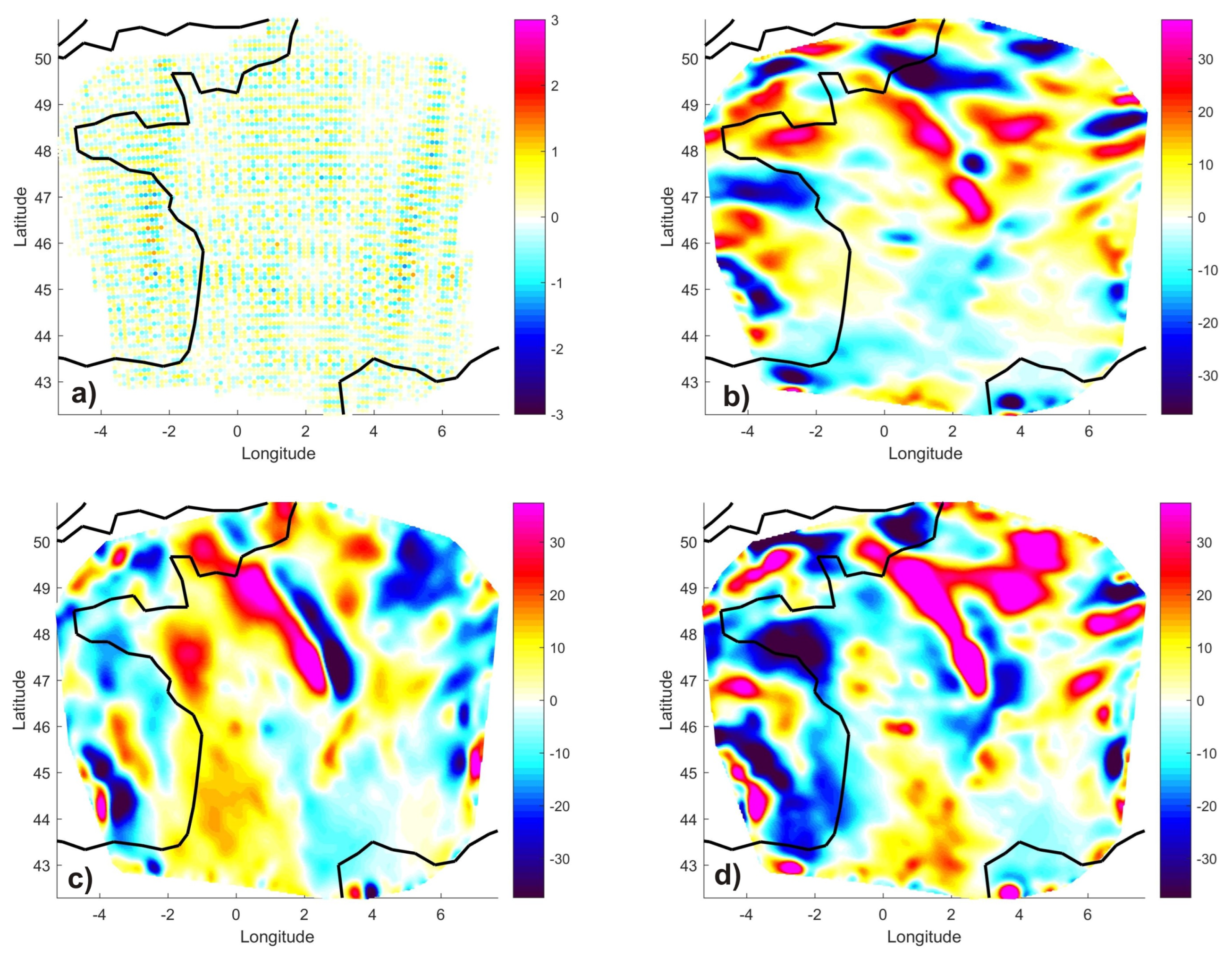
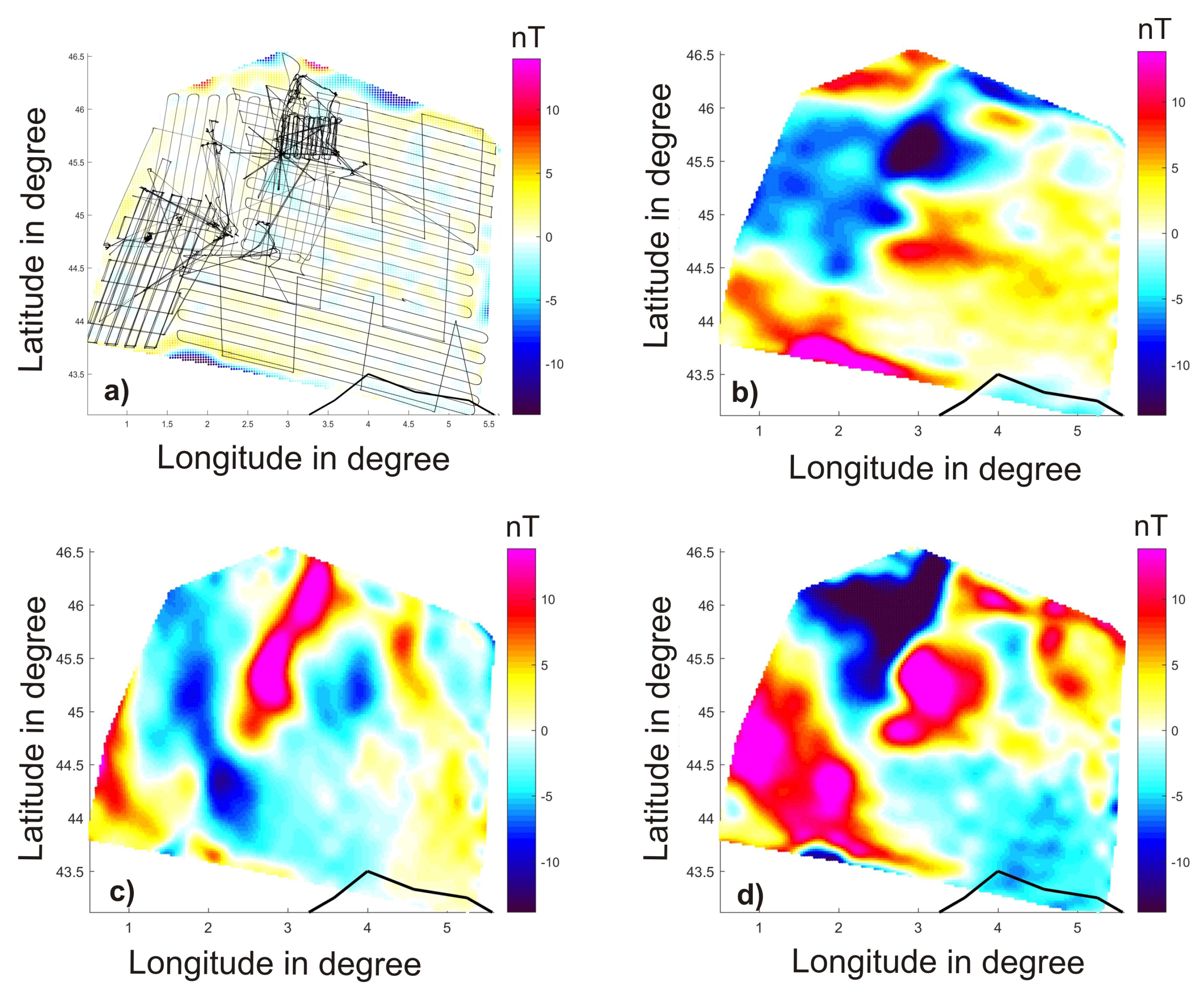
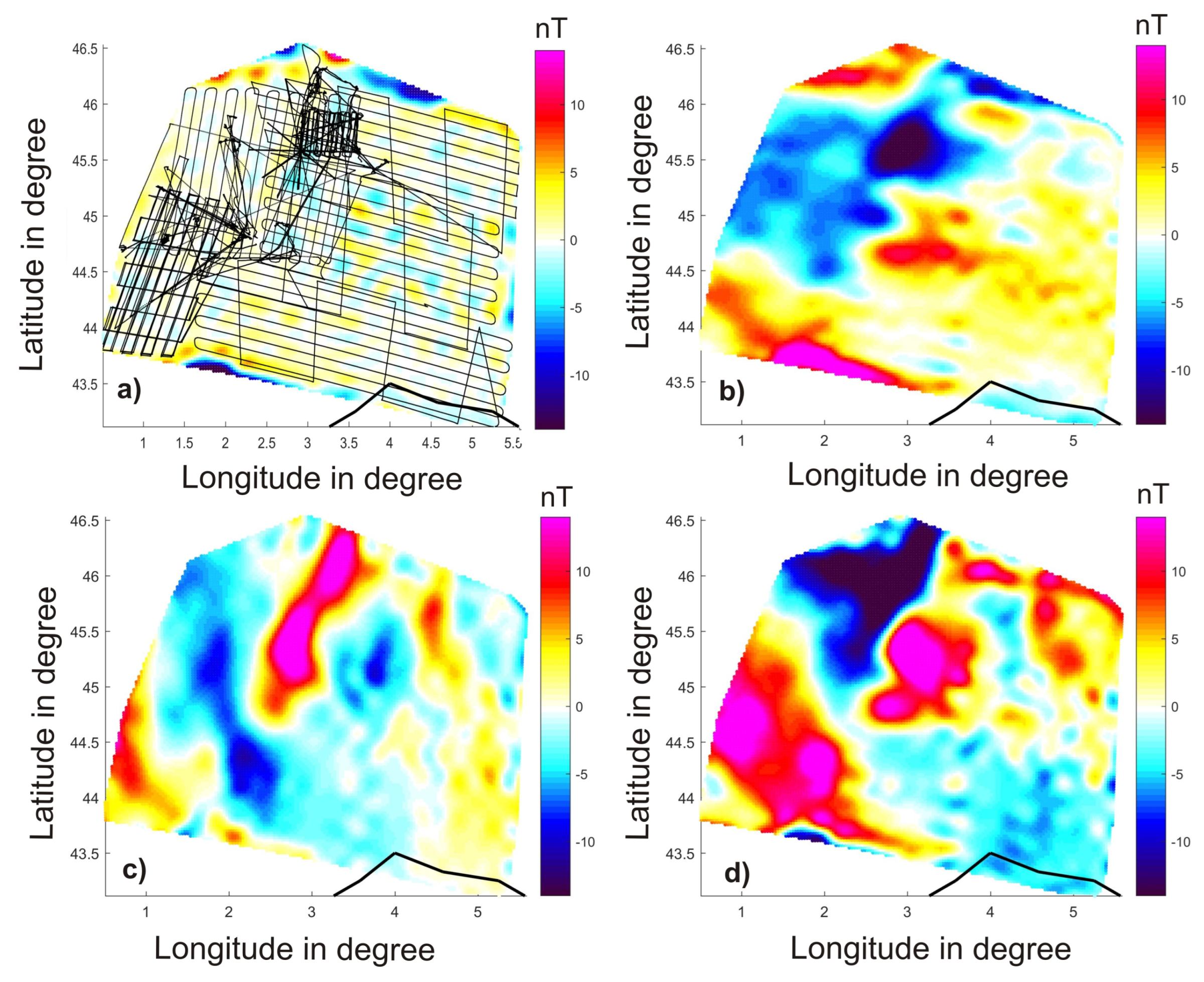
5. Results and Discussion

RHA models are derived from the three datasets described above. For the test case computed with the dataset SYN-AERO-PERFECT, we derive a model over France from the regular scalar anomaly grid to maximum expansion indices N = M = 30 in the infinite series (Equations (9a)–(9c)). For the inversion of datasets SYN-UAVS-PERFECT and SYN-UAVS-NOISED, the maximum truncation indices are set to N = M = 15 . According to Equation (8), the maximum spatial resolution for all three cases is about 30 km in the east and north directions. We remind the reader that the synthetic measurements were also computed with a global model to the maximum spatial resolution of about 38 km. Therefore, these RHA truncation indices correspond to the spatial information content of the synthetic measurements.
The residuals between the input scalar anomaly field computed in SYN-AERO-PERFECT and the RHA scalar anomaly model are displayed in Figure 5a after correcting for the constant field value. The global standard deviation of the inversion is 0.1 nT and most residuals correspond to oscillations typical of truncated double Fourier series. There is no increase of residuals near the edges, footprint of numerical ringing, or geometric distortion. The maps for three magnetic field components are predicted in the Cartesian reference frame at a constant altitude of 4 km above the Earth’s mean radius and converted back to the north (Figure 5b), east (Figure 5c), and vertical directions (Figure 5d) in the initial geocentric reference frame. The figures show that the model is stable and that it resolves the input measurements to the spatial resolution of the magnetic signal. One primary conclusion of this test is that RHA, which is a Cartesian representation, can be used to derive magnetic field models in the geocentric reference frame even when the curvature of the Earth cannot be neglected over extensions as large as 1000 km.
Regarding the realistic UAV data location experiments, the standard deviation between the synthetic measurements at their actual location and the RHA model predictions derived from the SYN-UAVS-PERFECT and SYN-UAVS-NOISED datasets are 0.2 nT and 1.5 nT, respectively. The misfit value for the RHA model based on the noisy dataset corresponds to the level of noise introduced in the dataset (Figure 4). The scalar and vector field models are then predicted on a regular grid at a constant altitude of 5 km above the Earth’s mean radius. Both residual maps between the intensity anomaly RHA predictions and the expected synthetic anomaly field values computed with the global spherical harmonic model [24] are displayed in Figure 6a and Figure 7a, respectively. The residuals show almost identical misfit patterns, with a comparatively larger amplitude for the model obtained with the noisy measurements. The vector field model derived from the SYN-UAVS-NOISED dataset is slightly noisier than the vector field model obtained with the SYN-UAVS-PERFECT one.
Figure 8a shows the initial geophysical noise (displayed as a time series in Figure 4 bottom) in the geographical frame that was added to the intensity data for the numerical simulation with the SYN-UAVS-NOISED dataset. This noise manifests itself as rapid spatial variations, along-flight errors, and data incompatibility in overlapping areas, but the algorithm identifies and downweights most of the noisy data (Figure 8b) during the inversion process. It should be noted that the geophysical noise we added comes from a magnetic field time series during a magnetic storm. With this signal being a time varying potential field, some of its contributions leak into the crustal field model in the geographic reference frame.
For both cases on UAV real trajectories there is no spatially coherent residuals between the model and the expected field, except near the edges where no measurement was available to build the RHA models. This indicates that the RHA models did not miss either large- or small-scale structures contained in the data. We remind the reader that intensity anomaly and vector field maps are leveled at the constant altitude of 5.2 km over a regular interpolation grid. The leveling altitude corresponds to the minimum altitude present in the dataset. Since the initial data altitudes comprise between 5.2 km and 20 km according to Figure 3b, the computation of the vector model corresponds to a downward continuation in all locations except for a small part of the southwest quadrant. Mapping the results at the minimum altitude was chosen for illustration purposes and does not correspond to the most advantageous scenario since downward continuation of potential fields is known to be prone to increased errors (e.g., [26]). The increased errors are due to the radial function that amplifies the smaller more than the larger length scales. We could have chosen another altitude for mapping the RHA model at a constant level (for example, at the median or the maximum data altitude); however, the maps obtained in these synthetic analyses from scalar measurements only are also stable for the three vector magnetic field components, and the magnetic field structures are spatially consistent.

6. Conclusions

The main incentive of this work was to process and to stitch together individual UAV surveys obtained in situ in order to build consistent magnetic field vector maps interpolated and leveled at a constant altitude. For this, an RHA mathematical representation was developed. Synthetic analyses based on closed-loop tests for three different case scenarios simulating real data distribution were carried out in order to demonstrate the ability of RHA to achieve this aim. It meets our initial needs to monitor and to quickly evaluate onsite the success of a magnetic survey, to filter out nonpotential field contamination signals, to verify the consistency between adjacent and/or surveys available at differing altitudes and epochs, to estimate the data noise level, and to identify in the geographical domain the series of problematic data acquisition. The synthetic analyses also demonstrate that the RHA approach can provide vector magnetic field models from scalar measurements acquired over large spatial extents such as aeromagnetic, airborne, and dense offshore marine magnetic surveys.
The RHA modeling method includes a processing block designed to minimize the effect of outliers and to reject measurements that do not obey the potential theory; however, the algorithm is not able to inform us about the origin of all possible contaminations. The reason is that UAV magnetic effects depend too strongly on each individual setup to allow the development of an automatic procedure (e.g., [27]). If it can readily be used for first-order in situ modeling, final robust magnetic field models must be obtained in the laboratory in a second step after further data analyses to correct for the systematic UAV magnetic bias and noise. In that regard, the algorithm provides useful guidance for their identification.
One limitation of RHA is its inability to separate the internal from the external magnetic fields and to deal with signals with wavelengths larger than the typical dimensions of the area under study. Such issues are, however, common to many regional potential field methods [5]. Beyond this standard limitation, one major outcome is that RHA is a mathematical potential field modeling approach. As such, it could be related analytically to physical parameters expanded in terms of double Fourier series such as pseudo-gravity anomalies, magnetic susceptibility distributions, or integrated magnetization models. This would directly, in situ, provide further and complementary information about the apparent physical properties of the magnetic sources.

Author Contributions

Conceptualization E.T. and L.-S.G.; mathematical formulation E.T.; methodology E.T. and L.-S.G.; data preparation E.T. and L.-S.G.; software E.T. and L.-S.G.; writing E.T. and L.-S.G. Both authors contributed equally to this research. All authors have read and agreed to the published version of the manuscript.

Funding

This work was funded partly funded by CNES in the framework of the project “Imagerie géophysique multi-échelles des édifices volcaniques” and the Agence National Research project Scan4Volc https://anr.fr/Project-ANR-21-CE49-0015, accessed on 10 September 2023. This is contribution no. 616 of the ClerVolc program of the International Research Center for Disaster Sciences and Sustainable Development of the University of Clermont Auvergne.

Data Availability Statement

The lithospheric magnetic field used for the synthetic analyses is available at https://swarm-diss.eo.esa.int/#swarm/Level2longterm/MLI/SW_OPER_MLI_SHA_2E_00000000T000000_99999999T999999_0801.ZIP, accessed on 10 September 2023. The auxiliary core field model CHAOS-7 is available at https://www.space.dtu.dk/english/research/scientific_data_and_models/magnetic_field_models, accessed on 10 September 2023. The synthetic datasets generated for this study and the code are available as an archive at https://www.opgc.fr/DOI/DataSoft/1qg6-qh39/RHA_optim_final.zip, accessed on 10 September 2023, under the Creative Commons licence with doi: https://doi.org/10.25519/1QG6-QH39, accessed on 10 September 2023.

Acknowledgments

We would like to thank the three anonymous referees for their constructive comments.

Conflicts of Interest

The authors declare no conflict of interest.

References

  1. Antoine, R.; Lopez, T.; Tanguy, M.; Lissak, C.; Gailler, L.; Labazuy, P.; Fauchard, C. Geoscientists in the sky: Unmanned aerial vehicles responding to geohazards. Surv. Geophys. 2020, 41, 1285–1321. [Google Scholar] [CrossRef]
  2. Hulot, G.; Sabaka, T.; Olsen, N. The present field. Treatise Geophys. 2007, 5, 33–75. [Google Scholar]
  3. Finlay, C.; Lesur, V.; Thébault, E.; Vervelidou, F.; Morschhauser, A.; Shore, R. Challenges handling magnetospheric and ionospheric signals in internal geomagnetic field modelling. Space Sci. Rev. 2017, 206, 157–189. [Google Scholar] [CrossRef]
  4. Zheng, Y.; Li, S.; Xing, K.; Zhang, X. Unmanned aerial vehicles for magnetic surveys: A review on platform selection and interference suppression. Drones 2021, 5, 93. [Google Scholar] [CrossRef]
  5. Schott, J.J.; Thébault, E. Modelling the earth’s magnetic field from global to regional scales. In Geomagnetic Observations and Models; Springer: Berlin/Heidelberg, Germany, 2010; pp. 229–264. [Google Scholar]
  6. Alldredge, L. Rectangular harmonic analysis applied to the geomagnetic field. J. Geophys. Res. Solid Earth 1981, 86, 3021–3026. [Google Scholar] [CrossRef]
  7. Vestine, E.H.; Davids, N. Analysis and interpretation of geomagnetic anomalies. Terr. Magn. Atmos. Electr. 1945, 50, 1–36. [Google Scholar] [CrossRef]
  8. Bhattacharyya, B. Two-dimensional harmonic analysis as a tool for magnetic interpretation. Geophysics 1965, 30, 829–857. [Google Scholar] [CrossRef]
  9. Alldredge, L.R. Geomagnetic local and regional harmonic analyses. J. Geophys. Res. Solid Earth 1982, 87, 1921–1926. [Google Scholar] [CrossRef]
  10. Haines, G. Regional Magnetic Field Modelling A Review. J. Geomagn. Geoelectr. 1990, 42, 1001–1018. [Google Scholar] [CrossRef]
  11. Huber, P.J. Robust Statistics; John Wiley & Sons: Hoboken, NJ, USA, 2004; Volume 523. [Google Scholar]
  12. Coddington, E.A.; Levinson, N.; Teichmann, T. Theory of Ordinary Differential Equations; McGraw-Hill Inc.: New York, NY, USA, 1956. [Google Scholar]
  13. Thébault, E.; Gaya-Piqué, L. Applied comparisons between SCHA and R-SCHA regional modeling techniques. Geochem. Geophys. Geosyst. 2008, 9, 7. [Google Scholar] [CrossRef]
  14. Haines, G. Spherical cap harmonic analysis. J. Geophys. Res. Solid Earth 1985, 90, 2583–2591. [Google Scholar] [CrossRef]
  15. Thébault, E. A proposal for regional modelling at the Earth’s surface, R-SCHA2D. Geophys. J. Int. 2008, 174, 118–134. [Google Scholar] [CrossRef]
  16. Thébault, E.; Schott, J.; Mandea, M. Revised spherical cap harmonic analysis (R-SCHA): Validation and properties. J. Geophys. Res. Solid Earth 2006, 111, B01102. [Google Scholar] [CrossRef]
  17. Blakely, R.J. Potential Theory in Gravity and Magnetic Applications; Cambridge University Press: Cambridge, UK, 1996. [Google Scholar]
  18. Backus, G.E. Non-uniqueness of the external geomagnetic field determined by surface intensity measurements. J. Geophys. Res. 1970, 75, 6339–6341. [Google Scholar] [CrossRef]
  19. Jiang, T.; Li, J.; Dang, Y.; Zhang, C.; Wang, Z.; Ke, B. Regional gravity field modeling based on rectangular harmonic analysis. Sci. China Earth Sci. 2014, 57, 1637–1644. [Google Scholar] [CrossRef]
  20. Lanczos, C. Applied Analysis; Dover Publication, Inc.: New York, NY, USA, 1988. [Google Scholar]
  21. Finlay, C.C.; Kloss, C.; Olsen, N.; Hammer, M.D.; Tøffner-Clausen, L.; Grayver, A.; Kuvshinov, A. The CHAOS-7 geomagnetic field model and observed changes in the South Atlantic Anomaly. Earth Planets Space 2020, 72, 1–31. [Google Scholar] [CrossRef]
  22. Le Mouel, J. Sur la Distribution des Elements Magnetiques en France. Ph.D. Thesis, University de Paris, Paris, France, 1969. [Google Scholar]
  23. Lesur, V.; Hamoudi, M.; Choi, Y.; Dyment, J.; Thébault, E. Building the second version of the world digital magnetic anomaly map (WDMAM). Earth Planets Space 2016, 68, 1–13. [Google Scholar] [CrossRef]
  24. Thébault, E.; Hulot, G.; Langlais, B.; Vigneron, P. A spherical harmonic model of Earth’s lithospheric magnetic field up to degree 1050. Geophys. Res. Lett. 2021, 48, e2021GL095147. [Google Scholar] [CrossRef]
  25. Gailler, L.; Labazuy, P.; Régis, E.; Bontemps, M.; Souriot, T.; Bacques, G.; Carton, B. Validation of a new UAV magnetic prospecting tool for volcano monitoring and geohazard assessment. Remote Sens. 2021, 13, 894. [Google Scholar] [CrossRef]
  26. Nabighian, M.N. Additional comments on the analytic signal of two-dimensional magnetic bodies with polygonal cross-section. Geophysics 1974, 39, 85–92. [Google Scholar] [CrossRef]
  27. Qiao, Z.K.; Yuan, P.; Wang, L.F.; Zhang, Z.H.; Huang, Y.S.; Zhang, J.J.; Li, L.L.; Zhang, Z.Y.; Wu, B.; Lin, Q. Research on aeromagnetic compensation of a multi-rotor UAV based on robust principal component analysis. J. Appl. Geophys. 2022, 206, 104791. [Google Scholar] [CrossRef]
Figure 1. Cartesian and geocentric reference frames and coordinate systems discussed in this paper. The rectangular prism is tangent to the Earth’s surface. Its center in the geocentric coordinate system is defined as the center of the available measurements. L x and L y are its dimensions in the north and east directions, respectively, and are defined according to the minimum and maximum geocentric data locations.
Remotesensing 15 04549 g001
Figure 2. General flowchart of the five main processing blocks generating a regional magnetic vector crustal field from raw UAV scalar intensity measurements. See text for details.
Remotesensing 15 04549 g002
Figure 3. (a) Crustal intensity anomaly field (in nT) over France and data location used for building the SYN-AERO-PERFECT dataset. (b) Crustal intensity anomaly field (in nT) at UAV data locations used for building the SYN-UAVS-PERFECT and SYN-UAVS-NOISED datasets. See text for details.
Remotesensing 15 04549 g003
Figure 4. Top: Magnetic intensity of the 23–24 April 2023 magnetic storm (in nT) recorded at the CMF ground magnetic station. Bottom: Residual signal after high-pass filtering that is added as a natural noise to build the SYN-UAVS-NOISED dataset.
Remotesensing 15 04549 g004
Figure 5. (a) Residual map (in nT) between the data and the RHA scalar anomalies predicted over France after modeling the SYN-AERO-PERFECT dataset. (b) Reconstruction of the magnetic north (b), the east (c), and the vertical component (d) of the crustal field. All maps are displayed in the geocentric reference frame at 4 km altitude above the Earth’s radius.
Remotesensing 15 04549 g005
Figure 6. (a) Residual map between the true and the RHA scalar anomalies over Massif-Central, France, predicted after modeling the SYN-UAVS-PERFECT dataset. (b) Reconstruction of the magnetic north (b), the east (c), and the vertical component (d) at the constant altitude of 5 km.
Remotesensing 15 04549 g006
Figure 7. (a) Residual map between the true and the RHA scalar anomalies over Massif-Central, France, predicted after modeling the SYN-UAVS-NOISED dataset. (b) Reconstruction of the magnetic north (b), the east (c), and the vertical component (d) of the crustal field at the constant altitude of 5 km.
Remotesensing 15 04549 g007
Figure 8. (a) Original noise introduced in the SYN-UAVS-NOISED dataset. (b) Misfit residuals between the model and the noisy data. (c) Difference between (a,b).
Remotesensing 15 04549 g008
Disclaimer/Publisher’s Note: The statements, opinions and data contained in all publications are solely those of the individual author(s) and contributor(s) and not of MDPI and/or the editor(s). MDPI and/or the editor(s) disclaim responsibility for any injury to people or property resulting from any ideas, methods, instructions or products referred to in the content.

