Article

HDM-RRT: A Fast HD-Map-Guided Motion Planning Algorithm for Autonomous Driving in the Campus Environment

State Key Laboratory of Information Engineering in Surveying Mapping and Remote Sensing, Wuhan University, Wuhan 430072, China
*
Author to whom correspondence should be addressed.
Remote Sens. 2023, 15(2), 487; https://doi.org/10.3390/rs15020487
Submission received: 23 November 2022 / Revised: 11 December 2022 / Accepted: 10 January 2023 / Published: 13 January 2023

Abstract

:
On campus, the complexity of the environment and the lack of regulatory constraints make it difficult to model the environment, resulting in less efficient motion planning algorithms. To solve this problem, HD-Map-guided sampling-based motion planning is a feasible research direction. We proposed a motion planning algorithm for autonomous vehicles on campus, called HD-Map-guided rapidly-exploring random tree (HDM-RRT). In our algorithm, A collision risk map (CR-Map) that quantifies the collision risk coefficient on the road is combined with the Gaussian distribution for sampling to improve the efficiency of algorithm. Then, the node optimization strategy of the algorithm is deeply optimized through the prior information of the CR-Map to improve the convergence rate and solve the problem of poor stability in campus environments. Three experiments were designed to verify the efficiency and stability of our approach. The results show that the sampling efficiency of our algorithm is four times higher than that of the Gaussian distribution method. The average convergence rate of the proposed algorithm outperforms the RRT* algorithm and DT-RRT* algorithm. In terms of algorithm efficiency, the average computation time of the proposed algorithm is only 15.98 ms, which is much better than that of the three compared algorithms.

1. Introduction

Autonomous vehicles (AVs) have been developed tremendously through the efforts of research institutes, universities and enterprises around the world. AVs can potentially improve the quality of the time spent in cars and increase the safety and efficiency of transportation systems [1]. Autonomous vehicles now successfully drive safely and stably on closed pre-approved roads in good weather; however, robust autonomous driving in urban traffic is still an unrealized goal [2]. In order to make AVs function in urban situations with unpredictable traffic, several real-time systems must interoperate [3], including high-definition maps (HD-Maps) [4,5], perception [6], localization [7,8], motion planning and control [9,10]. Motion planning, a basic component of autonomous driving, acts as a bridge between the decision and control modules and is indispensable for the safe and stable operation of AVs [11], by generating smooth and safe trajectories in the locally feasible solution space provided by the decision-making system.
Considerable attention has focused on feasible and optimal trajectory planning problems. Researchers have developed numerous motion planning algorithms and successfully applied them in specific autonomous driving scenarios. However, when it is applied to university campuses, the complexity of the environment and the lack of regulatory constraints make motion planning particularly challenging. The university campuses are typical widespread semi-enclosed environments where large numbers of staff and students live. There are more than 1.3 million college students living on university campuses in Wuhan, China. Wuhan University alone has more than 50,000 students and 10,000 faculty and staff living there. Autonomous driving applications such as self-driving buses, autonomous last-mile delivery logistics and unmanned patrol cars have large applications on campus [12,13,14]. University campus scenes are filled with narrow, semi-structured [15] roads and many obstacles, thus narrowing the access range. Figure 1 shows examples of the campus environment of Wuhan University.
Figure 1a is an HD-Map of the Wuhan University campus, and Figure 1b shows three scenes shot in it. There are narrow and irregular roads, unclear lane information and a large number of moving and stationary obstacles. Many electric bikes and vehicles are parked at random along the roadsides, destroying the original road boundaries. Bicycles and pedestrians on the campus do not necessarily follow the traffic rules, adding more uncertainty to the environment. In addition, the positioning accuracy of AVs on campuses is also very poor due to the large number of trees and buildings. These factors make it difficult to model the environment and also render the graph search motion planning algorithms that need to discretize the environment inefficient [16]. It is still a challenge for motion planning algorithms to achieve optimal real-time performance and high-quality trajectories for autonomous driving in campus scenes.
Sampling-based methods, as one of the most popular types of motion planning algorithms, are very effective in solving complex problems due to their strong exploration properties [17]. Sampling-based algorithms do not need to explicitly model obstacles in the state space, which saves a large amount of computation time. Recently, a large number of scholars have developed algorithms such as RRT, RRT *, Bi-RRT and DT-RRT [18,19,20,21], greatly promoting sampling-based algorithms’ applications in AVs. However, the complexity of campus scenes still restricts the algorithms’ efficiency and optimization. Due to the random nature of sampling-based algorithms, a large number of sampling iterations are needed to explore the environment to calculate the feasible trajectory, which will reduce the efficiency and stability.
In order to improve the computational efficiency and stability, sampling and node optimization strategies are the key factors. The sampling efficiency and node optimization speed can be greatly optimized using the prior information in the environment. As an important part of autonomous driving systems, HD-Maps can accurately provide AVs with prior information, including lane lines and road signs in the vector layer [22]. However, on the campus, the complexity of the environment and the lack of regulatory constraints make the traffic unpredictable. The prior information of a traditional navigation map is not enough to deal with this situation. To solve these problems, we combined HD-Maps with the artificial potential field (APF) method to generate a collision risk map (CR-Map) for sampling-based algorithms.
In our work, we optimized the motion planning module by combining an HD-Map and a sampling-based algorithm, aiming to quickly obtain high-quality, feasible trajectories in complex campus scenarios. A fast sampling-based algorithm is proposed for AVs in campus scenes, which is called the HD-map-guided rapidly-exploring random tree (HDM-RRT). The overall architecture of the proposed approach in this paper is shown in Figure 2.
As shown in Figure 2a, we generate the CR-Map through the vector layer of the HD-Map and the perception layer of the sensors, drawing on the idea of the APF method. The CR-Map can describe the risk coefficient of the collision between the autonomous vehicle and other obstacles on the road. The CR-Map is expressed in the form of a grid map, and each grid point has a collision risk coefficient. Regions with high collision risk coefficients are more dangerous than regions with low collision risk coefficients and will be given lower priority in the sampling space. Each node in our algorithm is assigned a collision risk coefficient. In the process of node optimization, the collision risk coefficient of each node is taken into account when calculating the cost function. The CR-Map can provide prior information and heuristic guidance for the sampling and node optimization processes. As shown in Figure 2b, we obtain sampling points in the sampling space through the CR-Map and Gaussian distribution. The CR-Map can provide heuristic guidance for the sampling process and improve the sampling efficiency of the algorithm. The sampling range and density are adjusted using the Gaussian distribution. The node optimization process in Figure 2c focuses on optimizing the parent–child relationship of the nodes in the tree. The cost function for determining the optimal parent node takes into account multiple factors such as the trajectory length, trajectory curvature and collision risk coefficient to improve the convergence rate of the algorithm. Moreover, the lane geometry information and traffic rule information provided by the HD-Map are used to constrain the node optimization process. Figure 2d shows examples of the sampling process, node optimization process and planned trajectory set.
The proposed algorithm significantly improves the sampling efficiency and convergence rate by optimizing the sampling and node optimization processes. Furthermore, the proposed algorithm reduces the iteration times and improves the computational efficiency while ensuring the trajectory quality. The four main contributions of this paper are as follows:
(1)
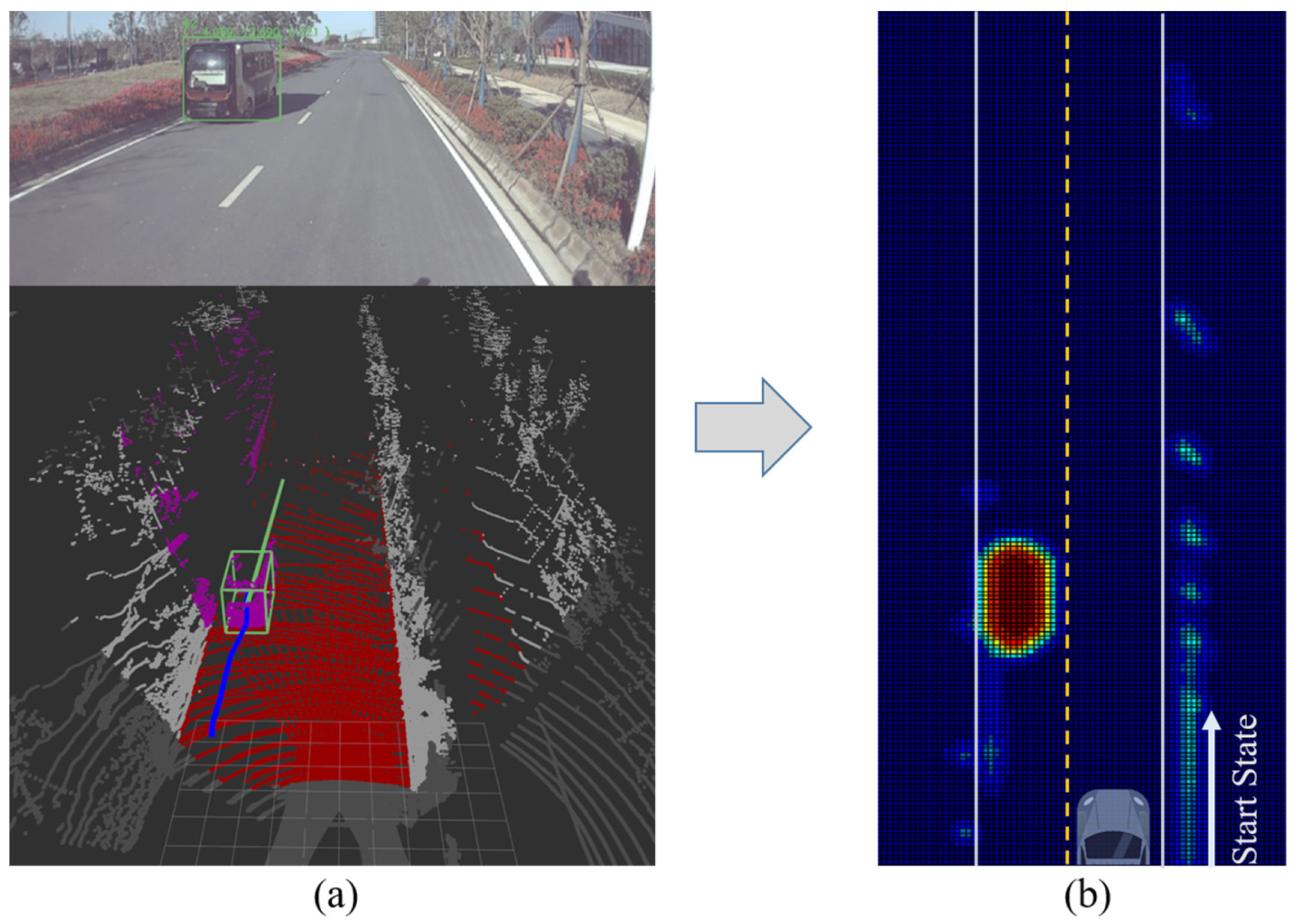
We propose a CR-Map layer to quantify the collision risk coefficient on the road, greatly expanding the prior information of the HD-Map to guide motion planning. The CR-Map is combined with Gaussian distribution for sampling, which significantly improves the efficiency of motion planning algorithms in campus scenes.
(2)
The node optimization strategy of the sampling-based algorithm is deeply optimized through the prior information of the CR-Map, which greatly improves the convergence rate, reduces the number of iterations and solves the problem of poor stability in campus environments.
(3)
The proposed HDM-RRT algorithm achieves optimal real-time performance and high-quality trajectories for autonomous driving in campus scenes. It is of great significance for applications such as self-driving buses, last-mile delivery logistics and unmanned patrol vehicles in campus and residential environments.
The remainder of this paper is organized as follows. Section 2 describes the related work of motion planning algorithms. Section 3 introduces the fundamentals including the data sources, the vehicle kinematic model and steering method, and the original RRT and RRT* descriptions. In Section 4, we describe the proposed CR-Map and HDM-RRT algorithm in detail. In Section 5, three experiments are conducted to compare the proposed HDM-RRT algorithm with the existing RRT*, DT-RRT* and dynEFWA-APF algorithms. Section 6 is the conclusion.

2. Related Work

In general, a motion planning module computes a feasible trajectory from the initial state of an AV to a goal state while satisfying the given kinodynamic and environmental constraints [19]. Researchers have developed numerous motion planning algorithms and successfully applied them in specific autonomous driving scenarios [23]. Motion planning algorithms can be broadly divided into two main categories according to the environmental modeling and searching strategy: graph search methods and sampling-based methods [17]. Graph search algorithms are a classic motion planning method and widely used in various applications such as robots, drones and AVs. A graph search algorithm discretizes the environment around the vehicle into a graph and searches the graph for the shortest path. Graph search algorithms include Dijkstra [24], A* [25] and the artificial potential field (APF) [26] method.
The Dijkstra algorithm is a shortest-path algorithm proposed in 1959. It performs a search to build a tree representing the shortest paths from a given root vertex to all other vertices in the graph. However, in a dense graph network, Dijkstra’s search efficiency is very low. A* is a heuristic search algorithm based on weighted graphs as an extension of the Dijkstra algorithm. A lot of research has been conducted to improve the efficiency of the A* algorithm [27,28,29]. The A* algorithm performs effectively on raster maps, but it is limited by the map resolution. The APF algorithm introduces the concept of physical fields into motion planning, where a target position generates an attractive field while obstacles generate repulsive fields [30]. In this way, a collision-free trajectory is calculated by searching the descending direction of the potential function from the initial point to the goal point. The simple structure and high computational efficiency of this algorithm make it widely applicable, but it easily falls into a local minimum point and often cannot achieve an optimum solution [31]. An improved APF algorithm based on a safety model analyzes the path planning mechanisms of human drivers [32]. This approach accounts for multiple traffic factors, making it suitable for AVs, but it has been verified only under ideal conditions on a structured road with a constant velocity. An optimization method based on dynEFWA and APF combined was proposed to plan a safe, smooth and dynamically feasible path for AVs [33]. However, this approach is still limited by the complexity of the environment.
The disadvantage of graph search algorithms is that they search over a fixed graph discretization; therefore, the trajectories can only be constructed from primitives. The graph resolution affects the motion planning effect, thus presenting an inescapable problem for graph search algorithms. At the same time, graph search algorithms cannot tackle complicated obstacle models in urban scenes as these scenes create modeling difficulties and reduce computational efficiency. Effective alternatives are sampling-based algorithms that can overcome the limitations of graph search approaches. Sampling-based methods sample points in the configuration space and incrementally build a reachability tree. When the tree is large enough to extend to the goal region, a feasible solution is found by tracing the edges to the starting state. Sampling-based methods are very effective in solving complex problems because of their strong exploration properties. The classical sampling-based algorithms include the rapidly-exploring random tree (RRT) [18] and RRT* [19].
The RRT algorithm was proposed as an efficient method for complex systems and has the characteristic of rapid exploration by taking a random sample in the configuration space and extending the tree in the direction of the sample. LaValle argued that the RRT algorithm is probabilistically complete, which means that a solution can be eventually found if it exists [34]. The RRT algorithm has attracted extensive attention because of its success in many tough scenes. Different from many other complete motion planning algorithms, the RRT framework does not need to explicitly model obstacles in the state space, which saves a large amount of computation time. Other than the explicit representation of the obstacles, the RRT algorithm only needs to employ a collision detector. This makes the RRT algorithm highly efficient for real-time autonomous driving systems [35] and particularly suited for problems with general differential constraints, complicated obstacle constraints and high degrees of freedom [36,37]. However, the RRT algorithm quickly obtains a feasible but suboptimal solution with no consideration of solution optimality [38].
The RRT* algorithm improves the RRT algorithm by solving the optimal problem, providing not only feasible but also asymptotically optimal solutions. The term asymptotically optimal means that the obtained trajectory continuously optimizes through increased sampling until converging to a global optimal solution. The RRT* algorithm converges with infinite samples but has no guarantees on their rate of convergence, resulting in low computational efficiency [39]. Dealing with complex scenes, when kinodynamic constraints are considered, the original RRT* algorithm cannot perform in real-time systems because of its slow convergence rate to the optimum.
Many researchers have proposed solutions to these RRT* problems. Some worked on improving the convergence rate [40,41], and others on non-holonomic systems [42,43]. A revised Gaussian distribution sampling-based RRT* algorithm was proposed that optimizes its sampling efficiency using the Gaussian distribution to avoid aimless full-plane sampling [44]. Nevertheless, its Gaussian sampling method does not optimize the convergence rate of the RRT* algorithm. Chen proposed a novel DT-RRT* algorithm utilizing a double-tree structure with high computational efficiency [21]. The double-tree structure includes an RRT tree and an RRT* tree. An RRT curve was generated as a reference path for the RRT* algorithm, achieving a fast convergence rate and a high-quality trajectory. However, this approach can only increase the convergence rate near the reference path; when the reference path generated via the RRT algorithm falls into a suboptimal solution, it is difficult for this method to achieve the optimum. Another double-tree RRT algorithm, Bi-RRT, was proposed and applied to various autonomous driving scenarios [45,46]. The Bi-RRT algorithm generates double trees from the initial and goal points simultaneously to increase the convergence rate of the algorithm. Some researchers enhanced the RRT algorithm performance by combining the APF algorithm and RRT [47,48,49]. These methods use the attractive and repulsive forces to offset the sampling points and nodes and provide better convergence rates. However, in complex scenes, the repulsive forces of obstacles are too complicated to model, resulting in the low efficiency of the algorithm.
The RRT and RRT* algorithms are effective for constraints such as complicated obstacles and narrow, semi-structured roads in autonomous driving systems, but they still have many problems including the suboptimal solution of RRT and the slow convergence rate of RRT*. In campus scenes, the low efficiency of the RRT* algorithm often fails to meet the real-time requirements. In harsh environments such as narrow entrances, it is also difficult for RRT* to quickly obtain the first feasible solution. Therefore, it is imperative to study how the algorithm efficiency can be improved while maintaining the quality of the trajectory. The main contributions and limitations of existing algorithms and our approach are shown in Table 1.
This paper draws on the idea of the artificial potential field method to generate a CR-Map using the vector layer of the HD-Map and the perceptual layer of the sensors. Through the prior information and heuristic guidance provided by the CR-Map, the sampling and node optimization processes of the sampling-based algorithm are improved to optimize the sampling efficiency and convergence rate. The next section presents the fundamentals of the proposed algorithm, with abbreviations listed in Table 2 for better readability.

3. Fundamentals of Algorithms

The proposed algorithm applies to real-time autonomous driving systems in campus scenes and uses various sensors of AVs such as the LIDAR, millimeter-wave radar, cameras and navigation systems. This section introduces the HD-Map used in our approach, the vehicle kinematic model and steering method, the definitions used in the motion planning problem and the original RRT and RRT* descriptions.

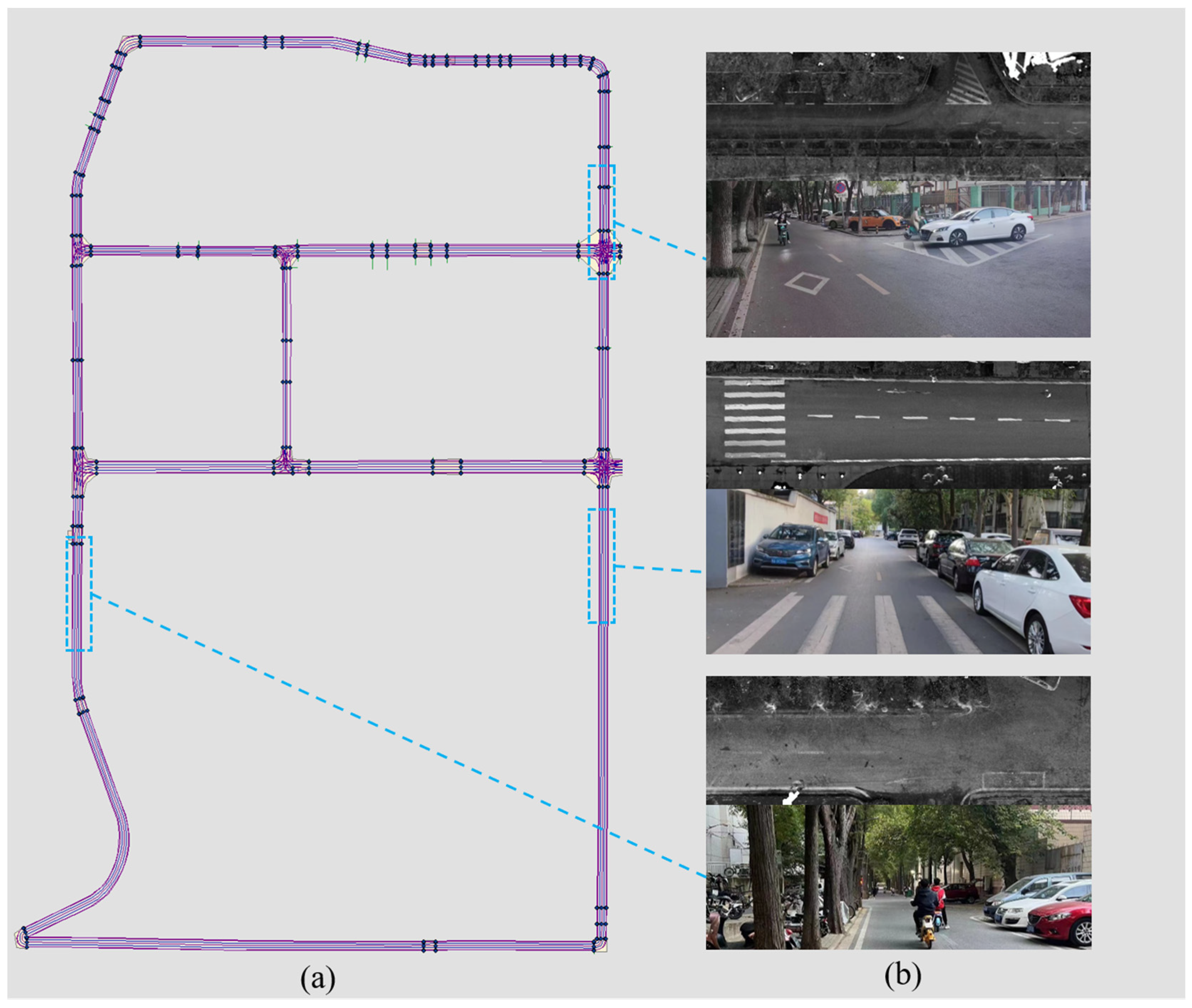
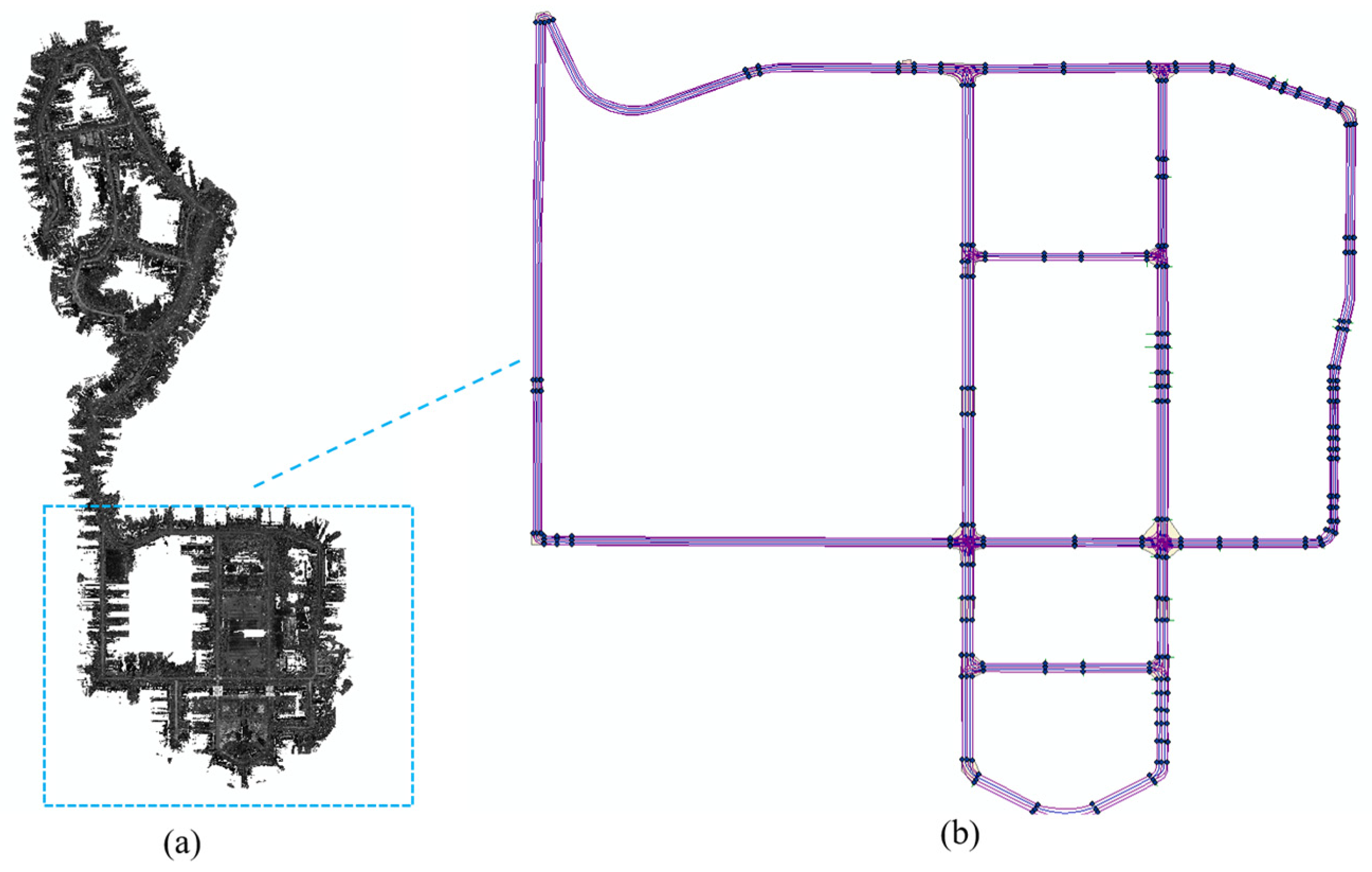
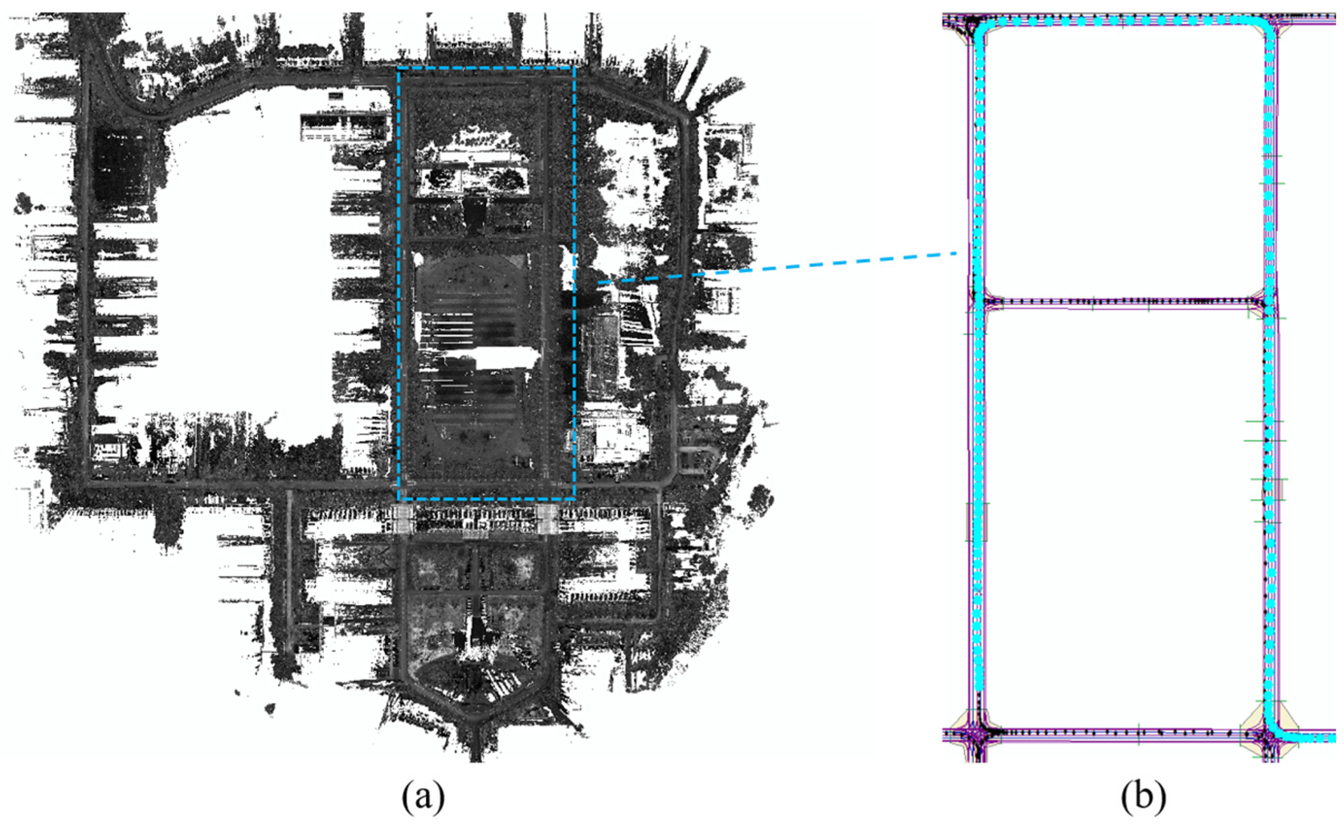
3.1. HD-Map of Wuhan University

This paper uses an HD-Map of Wuhan University independently developed by our team. The HD-Map contains a vector layer and a perception layer. The vector layer includes information such as topology, lane lines, lane midlines, intersections, sidewalks and stop lines. Figure 3 shows the HD-Map information of three campus scenes.
In Figure 3, the vector layer, perception layer and images of three scenes are shown. In the vector layer, the purple lines represent the lanes, the blue lines represent the midlines of the lanes and the blue dots are the topology points where the roads connect. The yellow areas are the junctions, the pink area is the sidewalk and the red lines are the stop lines. The vehicle kinematic model and steering method will be introduced in the next section.

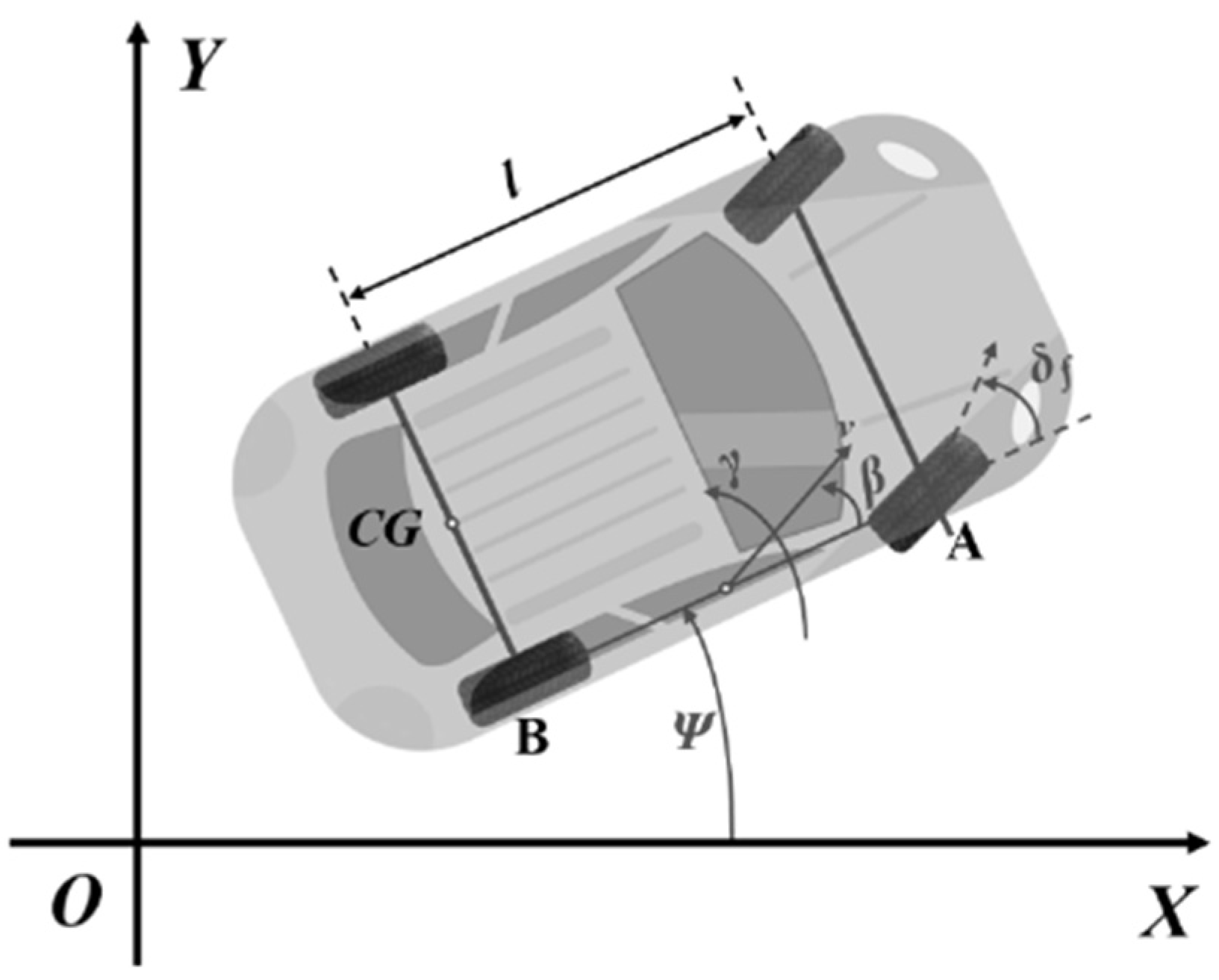
3.2. Vehicle Kinematic Model and Steering

The kinematic model of the vehicle is a factor that must be considered in motion planning. According to the Ackerman geometry, a vehicle’s kinematic model can be simplified to a two-wheeled model (bicycle model). The bicycle model takes a four-wheeled model and combines the front and rear wheels to form a two-wheeled model [50]. The kinematic model of the AV used in our approach is shown in Figure 4, and for better readability, the symbols in this paper are listed in Table 3.
In Figure 4, the vehicle’s state space is ( x , y , ψ ) X , where ( x , y ) represents the coordinates of mid-point of rear wheel, as shown by point CG. The ψ represents the intersection angle between the head direction and coordinate axis, l represents the wheelbase length. The kinematics of a front-steering vehicle can be expressed using Equation (1):
{ d x ( t ) d t = v ( t ) · c o s ψ ( t ) d y ( t ) d t = v ( t ) · s i n ψ ( t ) d v ( t ) d t = a ( t ) d ψ ( t ) d t = v ( t ) · t a n δ f ( t ) l d δ f ( t ) d t = w ( t )
In Equation (1), v represents the velocity of vehicle, a represents the corresponding acceleration, δ f represents the steering angle of front wheels and w refers to the corresponding angular velocity. w ( t ) and a ( t ) are control variables and the s ( x ( t ) , y ( t ) , ψ ( t ) ,   v ( t ) ,   δ f ( t ) ) are regarded as state variables. With their initial values known, the state variables will be determined one after another through integral provided. We set X o b s as the obstacle region, X f r e e = X / X o b s as the obstacle-free space, u ( w , a ) U as the control space, s i n i t , s g o a l and λ as the initial condition, goal region and feasible trajectory, respectively. Therefore, the motion planning problem can be described as follows: given an initial state s i n i t and a goal state s g o a l , find a feasible trajectory λ X f r e e and control input u U that satisfy the system constraints.
The steering procedure is crucial in the RRT-like algorithm, while the optimal controller is widely used to propagate a path from one point to another. Nevertheless, it is challenging to obtain a good input because it relies too much on the controllers’ quality. In this way, it makes the algorithm’s performance sensitive to the selection of the controllers and inputs, reducing the robustness. In our approach, we use a fast clothoid fitting method to compute the steering procedure, proven by Bertolazzi [51]. The clothoid curve is a G1 continuous curve generated using the Fresnel integral, and its curvature varies linearly with the arc. Shan developed a CF-pursuit algorithm to decrease fitting errors using the clothoid fitting method, proving that the clothoid curve is highly consistent with vehicle driving [52]. In addition, we also define the following terms for the rest of the paper:
(1)
C o l l i s i o n _ f r e e ( λ ) : checks the obstacle collision; if the λ is feasible, it returns true.
(2)
S a m p l e _ f r e e : returns a random sample point without collision.
(3)
N e a r e s t ( s , V ) : returns the node V closest to point s in the tree.
(4)
N e a r N o d e s ( V ) : returns the set of nodes near the node V in the tree.
(5)
S t e e r ( s 1 , s 2 ) : propagates a local path λ from point s 1 to point s 2 .
These terms will be used in the pseudocode, formulas and descriptions in the following sections.

3.3. Sampling-Based Algorithms: RRT and RRT*

The RRT* algorithm includes all the processes of the RRT algorithm and optimizes the node optimization strategy of the RRT algorithm. This section will describe the RRT* algorithm and its optimization process. The process of the RRT* algorithm is shown in Algorithm 1.
Algorithm 1: RRT*
1: Tree (Vxinit EØ);
2: while Flag_stop do
3:   xrand ← SampleFree;
4:   xnearestNearest(T = (V,E), xrand);
5:   xnew ← Steer(xnearest, xrand);
6:   costmin ←∞;
7:   if Collision_free(xnearest, xnew) then
8:       Xnearnodes ← NearNodes(T = (V,E), xnew);
9:       foreach xnear in Xnearnodes do
10:       Rewire (xnear, xnew, costmin);
11:     end
12:     VV {xnew};
13:     EE {(xnearest, xnew)};
14:     foreach xnear in Xnearnodes do
15:       if Rewire (xnew, xnear, costmin) then
16:         xparent ← Parent(xnear);
17:         EE{(xparent, xnear)}{(xnew, xnear)};
18:       end
19:     end
20:   end
21: end
In the RRT* algorithm, the tree T ( V , E ) is initialized first (Algorithm 1, row 1). Then, a random sampling point x r a n d in the X f r e e space is generated, and its nearest parent node in the tree is found, generating a new node x n e w through S t e e r ( x 1 , x 2 ) (Algorithm 1, rows 3–5). Next, if the point x n e w passes the collision detection, the X n e a r n o d e s in the tree are searched, and the optimal parent node is selected through the process R e w i r e (Algorithm 1, rows 9–11). Finally, the point x n e w is added to the tree, and then it is checked whether x n e w can be the parent of the node in X n e a r n o d e s (Algorithm 1, rows 14–19). If so, the parent–child relationship is modified (Algorithm 1, rows 16–17). The optimization of RRT* compared with RRT is that RRT* has the procedure of r e w i r e after x n e w is generated. The procedure for r e w i r e is described in Algorithm 2.
Algorithm 2: Rewire (x1, x2, costmin)
1: if cost(x1) + cost(Line(x1, x2)) < costmin then
2:   costmin ← cost(x1) + cost(Line(x1, x2));
3:   Return true
4: end
As can be seen in Algorithm 2, the rewire process compares the cost of x n e w to the root through different parent nodes, in order to determine the optimal parent node of x n e w . There are two rewire processes in RRT* (Algorithm 1, rows 11 and 17). The first one determines the parent node of x n e w , and the second one finds out whether x n e w can replace the parent node of other nodes. The second rewire process greatly reduces the efficiency of the algorithm because it needs to correct the relationship between the child and parent nodes in the tree. In the next section, we will introduce how the proposed HDM-RRT algorithm avoids this problem.

4. The Proposed HDM-RRT Algorithm

This section describes the proposed HDM-RRT algorithm in detail. The HDM-RRT algorithm includes the CR-Map, and the sampling, node optimization and trajectory optimization strategies. First, the CR-Map is proposed as an environmental model to describe the collision risk on roads. Then, we describe the structure of our approach and the sampling process. The cost functions for determining the optimal parent node and the optimal trajectory are described. Furthermore, the constraints and filters that respond to the requirements of the environment are discussed.

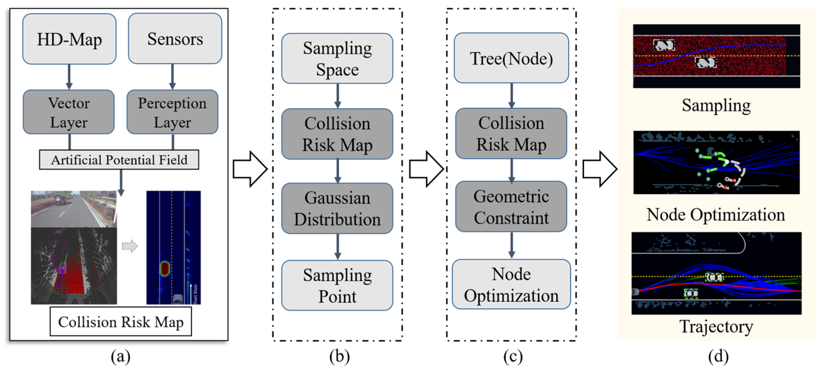
4.1. Collision Risk Map (CR-Map)

The CR-Map is an environmental model describing the collision risk on the road, represented in the form of a grid map. Based on the artificial potential field (APF) method, the CR-Map is constructed through the multi-source data, including the vector layer of the HD-Map and the perception layer of the sensors. A CR-Map example is shown in Figure 5.
Figure 5a shows the perception layer, and Figure 5b shows the CR-Map. In the CR-Map, the value of the collision risk for each grid point is represented. The collision risk values of different points in the CR-Map vary with the color. The dark-red points have large risk values, and the dark-blue points have small risk values. The collision risk values of the yellow and green points are between the dark-red points and the dark-blue points. The larger the grid point value on the CR-Map, the higher the risk of a vehicle collision. The maximum value is set to ten, and the minimum value is set to zero. When the collision risk of an area is 10, this area is inaccessible to a vehicle, as in the dark-red areas. When the collision risk of an area is zero, this area is feasible for a vehicle, as in the dark-blue areas in the map. The CR-Map construction method is described below.
To model the environment around the vehicle, a LIDAR point cloud is the basic data source. The driving environmental model includes the information of feasible road surfaces and the information of moving and stationary obstacles, where the accessible trajectory of the vehicle is planned on the road while avoiding obstacles. In the APF method, the obstacle in the state space generates repulsion when the target point generates attraction. We set obstacles on the road to create repulsive force, which means that they are inaccessible, and vehicles must avoid them. The road direction is more effective than the target point in a local plan, and it is not necessary to reach the target point of each plan. Therefore, in the CR-Map, we only need to consider the obstacle’s repulsive force, not the target point’s attractive force. Based on the above discussion, we set each grid point of obstacles on the map to exert a repulsive force on its surroundings, which is inversely proportional to the square of the distance. We use the repulsive field formula of the APF method to calculate the collision risk, as shown in Equations (2) and (3) [24]. The collision risk coefficient of each grid point on the CR-Map is calculated in Equation (4).
U r e p = { ρ 2 × ( 1 d ( q , q o b s ) 1 Q * ) 2 d ( q , q o b s ) Q * 0 d ( q , q o b s ) Q *
F r e p ( n ) P ( i , j ) = { ρ 2 ( 1 Q * 1 d ( P ( i , j ) , P ( n ) ) ) 1 d ( P ( i , j ) , P ( n ) ) 2   d P ( n ) d ( P ( i , j ) , P ( n ) ) Q * 0 d ( P ( i , j ) , P ( n ) ) Q *
        F r e p P ( i , j ) = n F r e p ( n ) P ( i , j ) , i f ( F r e p P ( i , j ) > F max ) , F r e p P ( i , j ) = F max
where U r e p represents the repulsive force field, ρ represents the coefficient, d ( q , q o b s ) is the distance between the grid point and obstacle and Q * is the obstacle influence radius. When the distance is greater than Q * , the obstacles’ influence on the grid point is considered zero. For any point P ( i , j ) and obstacle point P ( n ) to be measured in the grid space, d ( P ( i , j ) , P ( n ) ) is the distance between the grid point P ( i , j ) and obstacle P ( n ) , d P ( n ) is the partial derivative vector of the distance from the P ( n ) to the P ( i , j ) . The repulsive force of the P ( n ) to P ( i , j ) is F r e p ( n ) P ( i , j ) , and the total repulsive force F r e p P ( i , j ) is the sum of the repulsive force of each obstacle point. In our road CR-Map, repulsion is used to calculate the cost function for determining the optimal trajectory instead of changing the location of sampling points or existing tree nodes. Hence, we only consider the intensity not the direction of the repulsion. The repulsive force F r e p P ( i , j ) generated by multiple obstacle points on the same grid is superimposed by addition, and the maximum value of the repulsive force of grid points is F m a x , which is set to 10. When the value of   F r e p P ( i , j ) is 10, the grid is the dark-red areas in Figure 5b. When the value of   F r e p P ( i , j ) is 0, the grid is the dark-blue areas in Figure 5b. When the repulsive force value of the grid point is greater than F m a x , it is set to F m a x . After obtaining the repulsive force field, it is necessary to fuse the road and traffic information of the HD-Map to generate the CR-Map and obtain the collision risk coefficient of each grid point.
The CR-Map supports the sampling, node optimization and trajectory optimization processes. The sampling uses the Gaussian distribution based on the CR-Map coefficient. The cost functions for selecting the optimal parent node and optimal trajectory also consider the collision risk coefficient in the CR-Map. Each trajectory in the CR-Map has a risk value, called CR-Cost, which is obtained by adding the risk coefficient for each grid on this trajectory. The structure of HDM-RRT will be described in Section 4.2.

4.2. Structure of the Proposed HDM-RRT Algorithm

The proposed HDM-RRT algorithm is an improved sampling-based algorithm based on a CR-Map. The difference between our approach and the original RRT algorithm lies in the sampling, node optimization and cost function to determine the optimal parent node and the optimal trajectory. The framework of the HDM-RRT algorithm is shown in Algorithm 3.
Algorithm 3: HDM_RRT*
1: Tree (Vxinit EØ);
2: xrandCR_GussianSampling;
3: xnearnodes ← Nearest(T = (V, E), xrand);
4: foreach xnear in xnearnodes sort() do
5:   xnew = Steer(xrand, xnearnodes);
6:   if constrains_check() then
7:     xtemp = xnear;
8:     Break;
9:   end
10: end
11: xnearnodes ← Nearest(T = (V,E), xnew);
12: foreach xnear in xnearnodes do
13:   if cost(xnew) < costmin && constrains_check() then
14:     costmin ← cost(xnew)
15:     xtemparent = xnear;
16:   end
17: end
18: xtemp = xtemparent;
19: while xtemp!= xinit do
20:   xtemp = xtemp.getparent();
21:   if cost(xtemp) + cost(xtemp, xnew) < costmin && constrains_check() then
22:     Costmin ← cost(xtemp) + cost(xtemp, xnew);
23:     xfinalparent = xtemp;
24:   end
25: end
26: VV {xnew}; EE {(xfinalparent, xnew)};
27: Flag_add = true;
In Algorithm 3, the tree T ( V , E ) is initialized first (Algorithm 3, row 1). To obtain x r a n d , we propose CR_GaussianSampling by combining the Gaussian distribution and CR-Map to improve the sampling efficiency of the algorithm (Algorithm 3, row 2). The sampling strategy will be described in Section 4.2.1. After generating a random sample point x r a n d , we use the Euclidean distance to find a series of tree nodes closest x n e a r n o d e s to the sample point and sort them by distance (Algorithm 3, rows 4–10). Starting from the nearest tree node, obstacle detection and kinodynamic constraint detection are carried out one by one; thus, the passing nodes are taken as candidate parent nodes. The parent node does not directly match the nearest node of the new node but searches from a point set to avoid selecting the invalid parent node.
After obtaining the temporary parent node of the new node x t e m p , we propose a new method to replace the original r e w i r e method in RRT*, dividing it into two steps. The first step is to find the nearby node set of the new node and then calculate the optimal parent node x t e m p a r e n t using the new cost function, which takes the CR-Map coefficient into account (Algorithm 3, rows 12–17). The second part traces the optimal parent node of the new node to the root point to find out whether there is a better parent node x f i n a l p a r e n t (Algorithm 3, rows 19–25). There are also two r e w i r e processes in the original optimization process of RRT*; in particular, the second R e w i r e ( x n e w , x n e a r ) needs to modify each child node of x n e a r , requiring a huge amount of calculation. Compared with RRT*, the HDM-RRT method is similar to a shortcut method, improving the computational speed and reducing the redundancy and tree depth. The new rewire method of the node optimization is shown in Section 4.2.2. If the above steps pass the obstacle detection and constraint checks, the new node is pushed into the tree T ( V , E ) (Algorithm 3, row 26). Finally, the method checks whether the new node can extend directly to the goal point and satisfy the constraints. If the result is satisfied, this indicates that a feasible trajectory has been generated.

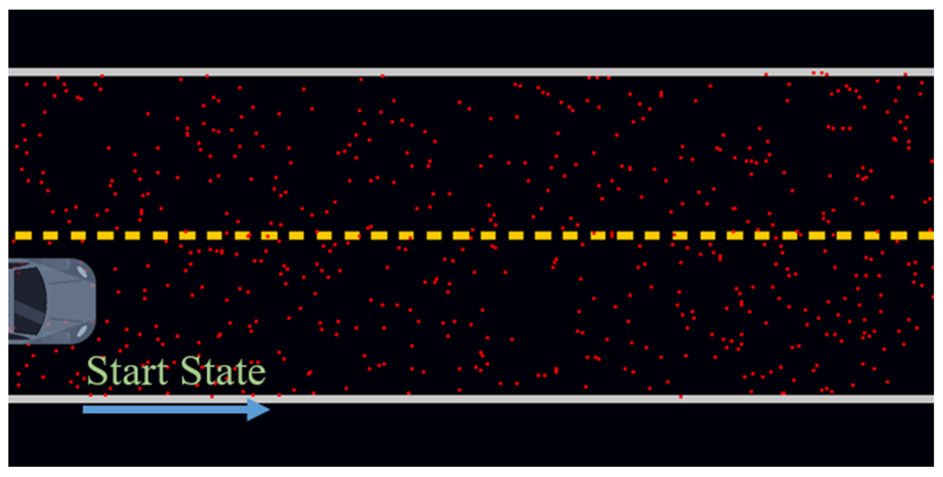
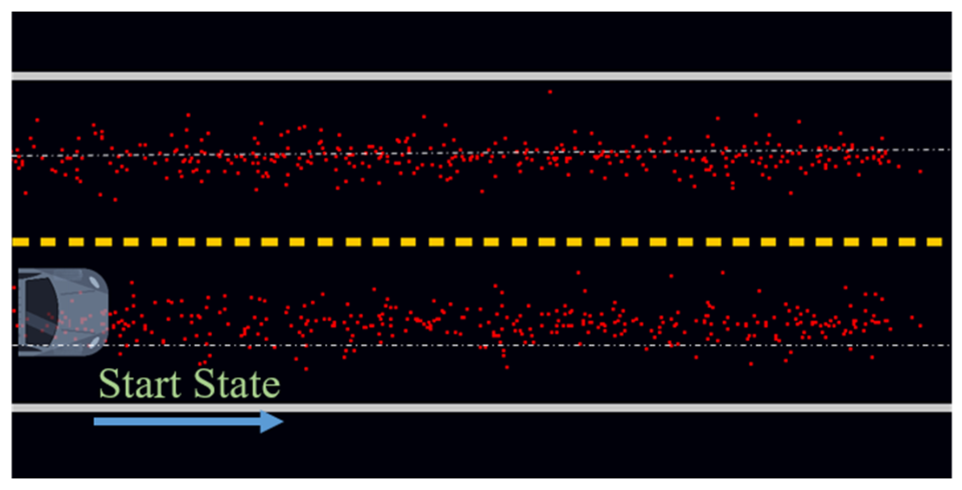
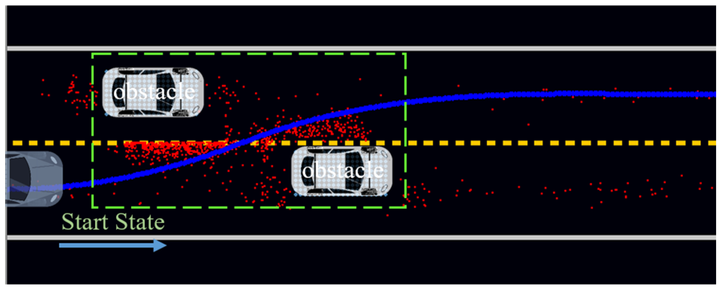
4.2.1. Sampling Strategy

The random distribution sampling method is widely used in sampling-based algorithms, as shown in Figure 6. The red points are the sampling points. It can be seen in Figure 6 that the sampling points obtained by the random distribution sampling method are uniformly distributed in the configuration space, which makes this random method very inefficient.
Gaussian distribution sampling requires a reference point and a reference line, and the sampling points are distributed near the reference point. The distribution range of sampling points can be adjusted by changing the parameters of the Gaussian distribution. The sampling method based on the Gaussian distribution takes the center line of the lane as the reference line and randomly selects a reference point on that line. The obtained sampling points are shown in Figure 7. Most of the points sampled using the Gaussian method are distributed near the center line of the two lanes, while a few points are distributed relatively far from the center line of the lanes.
When there are obstacles in the environment, as shown in Figure 8, the primary task of motion planning is to avoid obstacles. In this scenario, the AV has to avoid obstacles to change lanes, and the blue curve is the trajectory. Our area of interest (AOI) is between the two obstacles, as shown in the green box. When the sampling points are concentrated in the AOI, it is easier to avoid obstacles and find feasible trajectories. In order to sample more points in the AOI, a sampling method that combines the CR-Map and Gaussian distribution is proposed, as shown in Algorithm 4.
Algorithm 4: CR_GussianSampling
1: x0, y0, θ0 = GetReferencepoint();
2: do
3:   Radiusrandom, θrandom = BoxMuller();
4:   Radius = σradius * abs(Radiusrandom);
5:   θ = σθ * θrandom + θ0;
6:   RandomPoint.x = x0 + Radius * cos(θ);
7:   RandomPoint.y = y0 + Radius * sin(θ);
8: while (rand(max_risk) < CRcoefficient(RandomPoint));
In Algorithm 4, the reference point of the Gaussian distribution is obtained first (Algorithm 4, row 1). The sampling range can be controlled through the selection of control reference points. In the CR-Map, the value of each grid point represents the collision risk coefficient. The grid points in the obstacle area have the highest value, and those in the area away from the obstacle have the lowest value. Therefore, the area of gradient descent in the CR-Map is the surrounding region of the obstacles. In the proposed method, we increase the probability of selecting the point in the gradient descent region as the reference point. Next, the Box–Muller algorithm is employed to obtain Gaussian-distributed random numbers. Two Gaussian random numbers, R a d i u s r a n d o m and θ r a n d o m , are calculated using the Box–Muller model (Algorithm 4, row 3). From this, we can calculate the Radius and θ (Algorithm 4, rows 4–5), where σ r a d i u s and σ θ represent the range radius and angle of the sampling. After that, the random point can be computed using trigonometric functions (Algorithm 4, rows 6–7). The calculated random point must be projected into the CR-Map to calculate its collision risk coefficient (Algorithm 4, row 8). Taking the CR-Map coefficients into account, a random point is discarded if its collision risk value is higher than the generated random risk value. As shown in Figure 9, the proposed sampling method significantly increases the number of samples in the key area near the obstacles.
After introducing the sampling method, the node optimization strategy of the proposed HDM-RRT algorithm is introduced in detail. It includes the strategy of selecting the optimal parent node, the cost function of determining the optimal parent node and the cost function of determining the optimal trajectory.

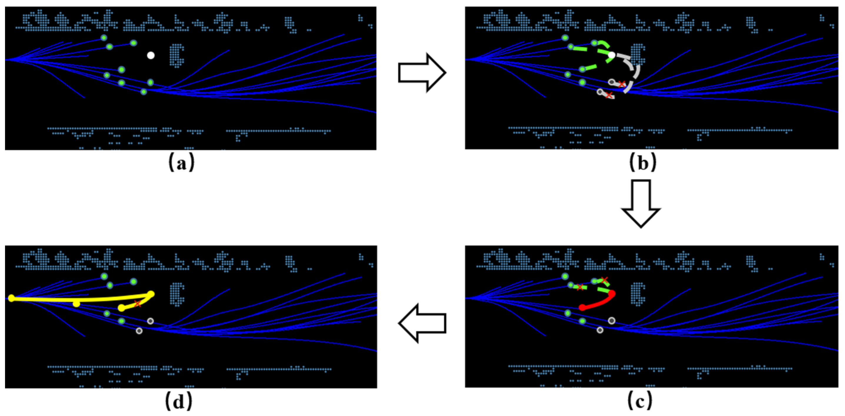
4.2.2. Node Optimization Strategy

The node optimization of our approach is to calculate the optimal parent node of the new node and avoid excessive computation. Different from RRT*, the search strategy of the proposed HDM-RRT is similar to a shortcut method, improving the computational speed, and reducing the redundant branches and tree depth. Our search strategy for selecting the optimal parent node is divided into four steps, as shown in Figure 10.
In Figure 10a, a series of points closest to the sampling point in the tree are searched as candidate parent nodes. The white node is the random sampling point x r a n d , while the green nodes are the candidate parent nodes near the sampling point. In Figure 10b, the trajectories of the candidate parent nodes are projected to x r a n d through the steer process. The collision detection, vehicle kinematic constraint detection and environment constraint detection of the trajectories are taken to eliminate the unsuitable points. The gray nodes are the disqualified parent nodes, while the green nodes are the available parent nodes. After obtaining the potential parent nodes, the optimal parent node is selected through the global cost of different parent nodes to the root node. The red nodes in Figure 10c are the successfully paired parent nodes and sampling points x r a n d . In Figure 10d, from the current optimal parent node tracing back to the root node, the global cost function is used to calculate whether there is a better parent node. The connected yellow nodes are the parent and child nodes that are finally paired successfully. When calculating the optimal parent node and the optimal trajectory, the cost functions must be considered.
The cost functions in our approach are designed by incorporating multiple factors such as the trajectory length, trajectory curvature and CR-Map coefficient. In the CR-Map, each grid has a CR-Map coefficient, so we can obtain the CR-Cost of any trajectory. We fuse the CR-Cost and trajectory length cost in a weighted way to select the optimal parent node, as shown in Equation (5):
n e w c o s t _ n ( x 1 , x 2 ) = δ c r C R _ c o s t ( x 1 , x 2 ) + δ l l e n g t h ( x 1 , x 2 )
where, after normalization, C R _ c o s t ( x 1 , x 2 ) is the CR-Map coefficient of the trajectory from x 1 to x 2 , l e n g t h ( x 1 , x 2 ) is the travel distance of the trajectory from x 1 to x 2 , and δ c r and δ l are the weights of the CR-Cost and trajectory length cost, respectively. The cost function to select the optimal trajectory is described in Equation (6):
n e w c o s t _ t ( t 1 ) = δ c r C R _ c o s t ( t 1 ) + δ l l e n g t h ( t 1 ) + δ k c u r v a t u r e ( t 1 )
where, after normalization, C R _ c o s t ( t 1 ) is the CR-Map coefficient of trajectory t 1 , l e n g t h ( t 1 ) is the travel distance of trajectory t 1 , c u r v a t u r e ( t 1 ) is the curvature index of trajectory t 1 , and δ c r , δ l and δ k are the weights of the CR-Cost, trajectory length cost and curvature cost, respectively.

4.2.3. Constraints and Filters

HDM-RRT is designed for autonomous vehicles, so the vehicle kinematic model and traffic constraints have to be considered to filter out some unqualified nodes in the algorithm. The vector layer of the HD-Map and vehicle parameters are used as a basis for the constraints. These include the curvature, detour and turning radius constraints.
(1)
Curvature constraint: The Dubins curve is one of the most widely used trajectory methods in autonomous driving, but its curvature is not continuous, which is not conducive to the stability of AVs. The clothoid curve is employed to generate the trajectory from state A to state B. As discussed in Section 3.2, the clothoid curve is a G1 continuous curve generated using the Fresnel integral. Unlike the curvature discontinuities of the Dubins curve, the curvature of the clothoid curve varies linearly with the arc. Studies have shown that the clothoid curve is highly consistent with vehicle driving [45]. In calculating the clothoid curve, it is easy to obtain the curvature of the starting point and goal point, and the curvature rate. By limiting the curve curvature, the trajectory quality can be controlled effectively and fit the vehicle steering model.
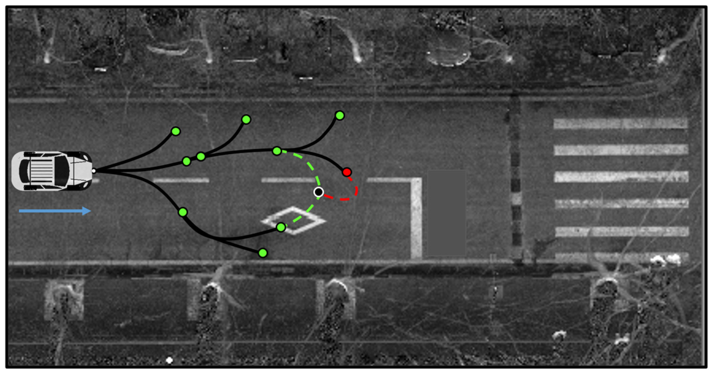
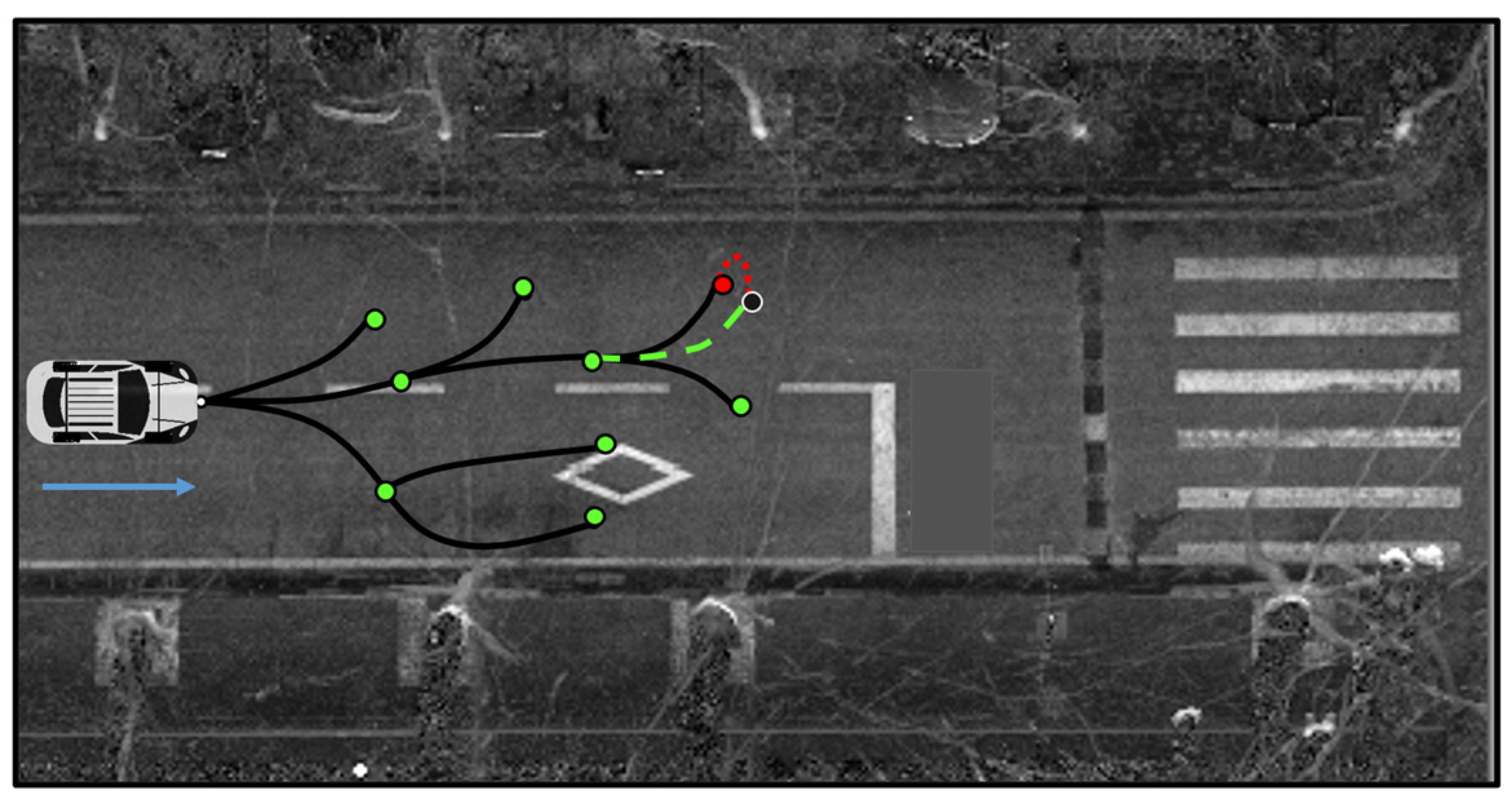
(2)
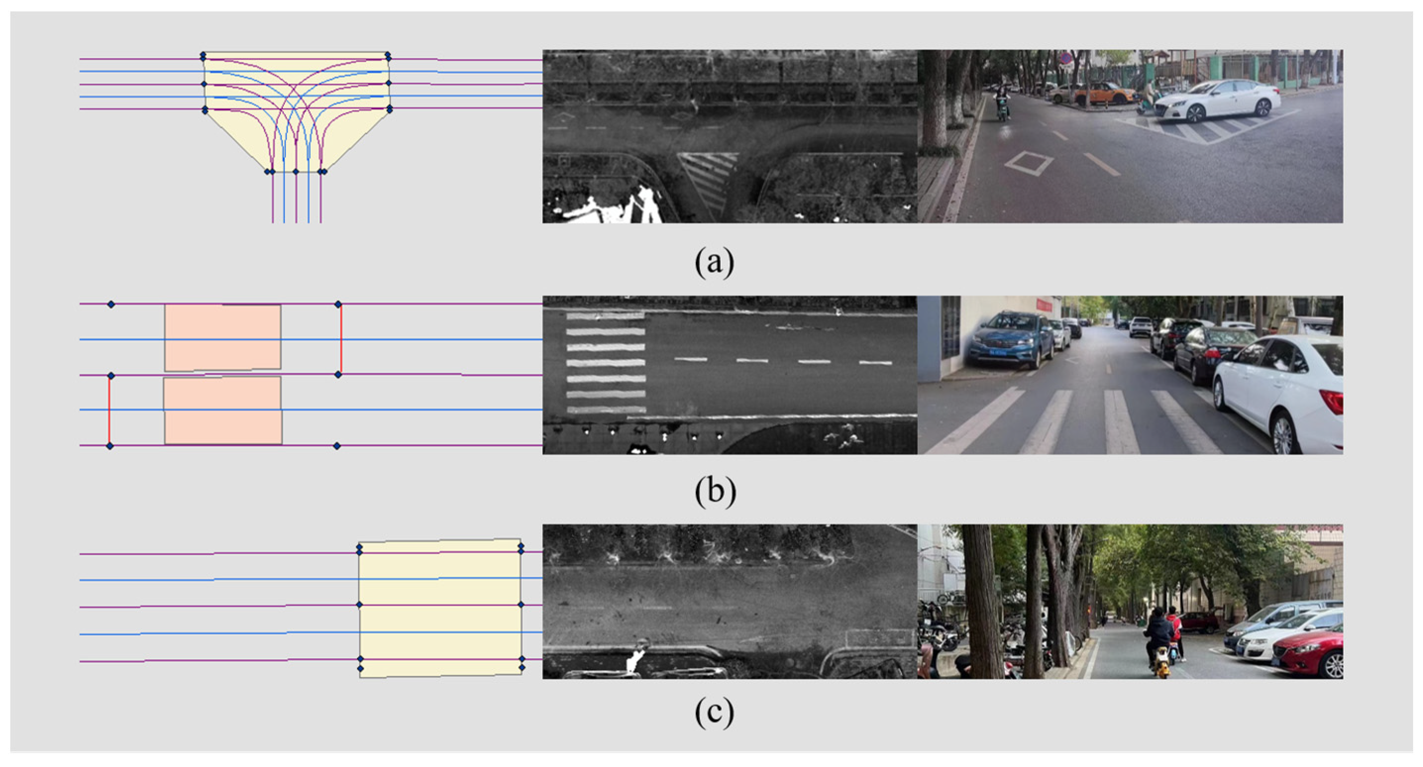
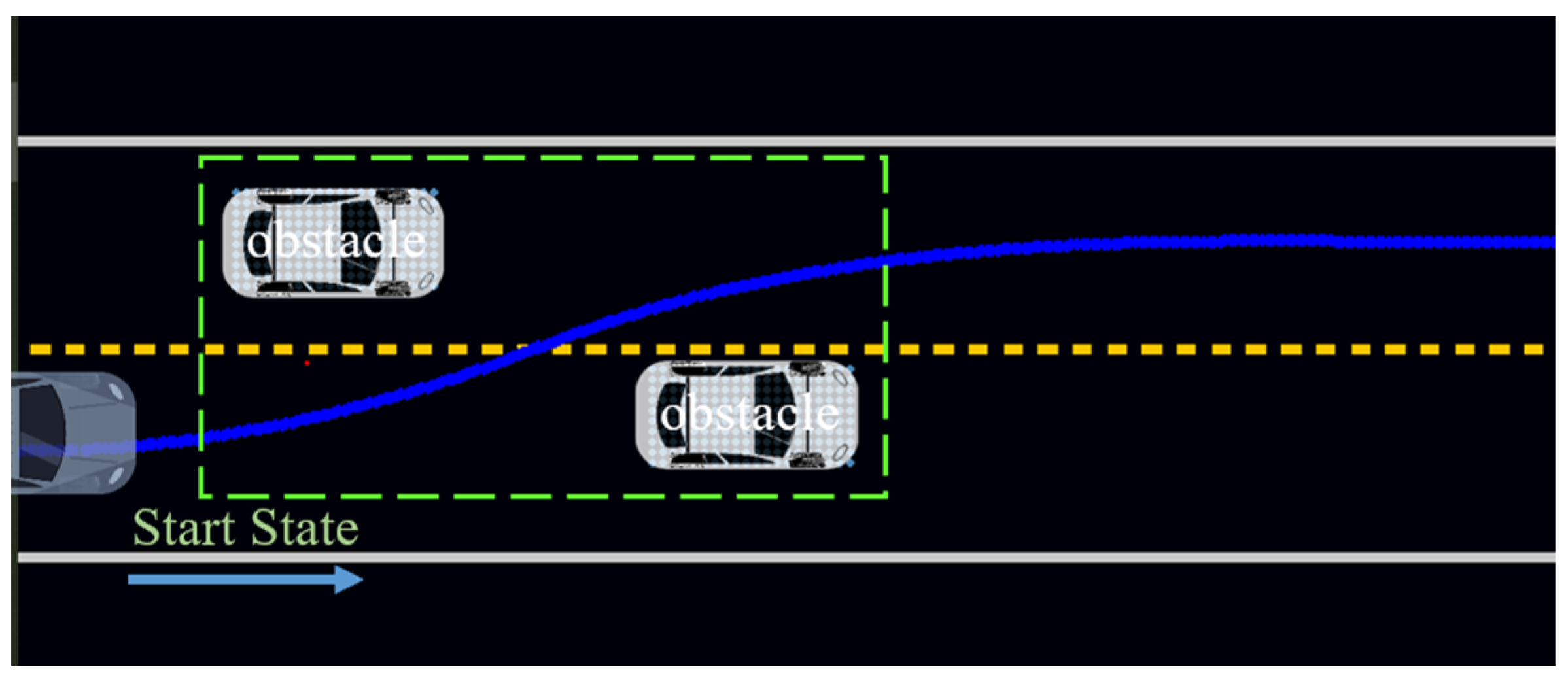
Detour constraint: In actual traffic scenes, roads are directional. When driving a vehicle on the road, it must comply with the traffic rules’ constraints and cannot be turned around at will. Therefore, we added a circuitous constraint here. It is required that the sampling point should not select a node whose relative direction is opposite to the road direction. The schematic diagram is shown in Figure 11.
As shown in Figure 11, the black points are our sampling points, and the nodes connected by the green and red dotted lines are the parent nodes to be selected. The red parent node is disabled because it is opposite to the sampling point direction of the road.
(3)
Turning radius constraint: The trajectory needs to meet the kinodynamic constraints of the vehicle when driving, and each vehicle has its turning radius. Therefore, it is necessary to add the constraint of the vehicle’s turning radius to the curve so that the vehicle can pursue the planned trajectory better, as shown in Equation (7):
Δ S > Δ θ k m a x
In Equation (7), we set the angle difference between the sampling point and parent node as Δ θ , their arc length as Δ S and the maximum curve curvature as k m a x . An example of the turning radius constraint is shown in Figure 12.
In Figure 12, the red node connected by the red dotted line does not satisfy the vehicle’s turning radius requirements, so it is removed. On the contrary, the node connected by the green dotted line satisfies the requirements and can be selected as the parent node.

5. Experiments and Analysis

5.1. Experimental Design

5.1.1. Experimental Purpose

The purpose of the experiments was to verify the effectiveness of the proposed algorithm in improving the sampling efficiency, accelerating the convergence rate and reducing the number of iterations of the sampling-based algorithm. Moreover, the experiments also verified that the proposed algorithm is competent for autonomous driving in campus scenes. In order to achieve these experimental purposes, we designed three experiments. First, we obtained vector layer and perception layer data of the campus road. We compared the sampling efficiency of the original random-distribution sampling method, the improved Gaussian-distribution sampling method and the proposed sampling method based on the combination of the CR-Map and Gaussian distribution. Second, we ran three motion planning methods on the road for 100 times, namely, the original RRT* algorithm, the improved DT-RRT* algorithm and the algorithm proposed in this paper, and compared the average number of iterations, the number of nodes and the number of trajectories of these three algorithms. Third, we ran an autonomous vehicle on the road and compared the average time taken by the four motion planning algorithms.

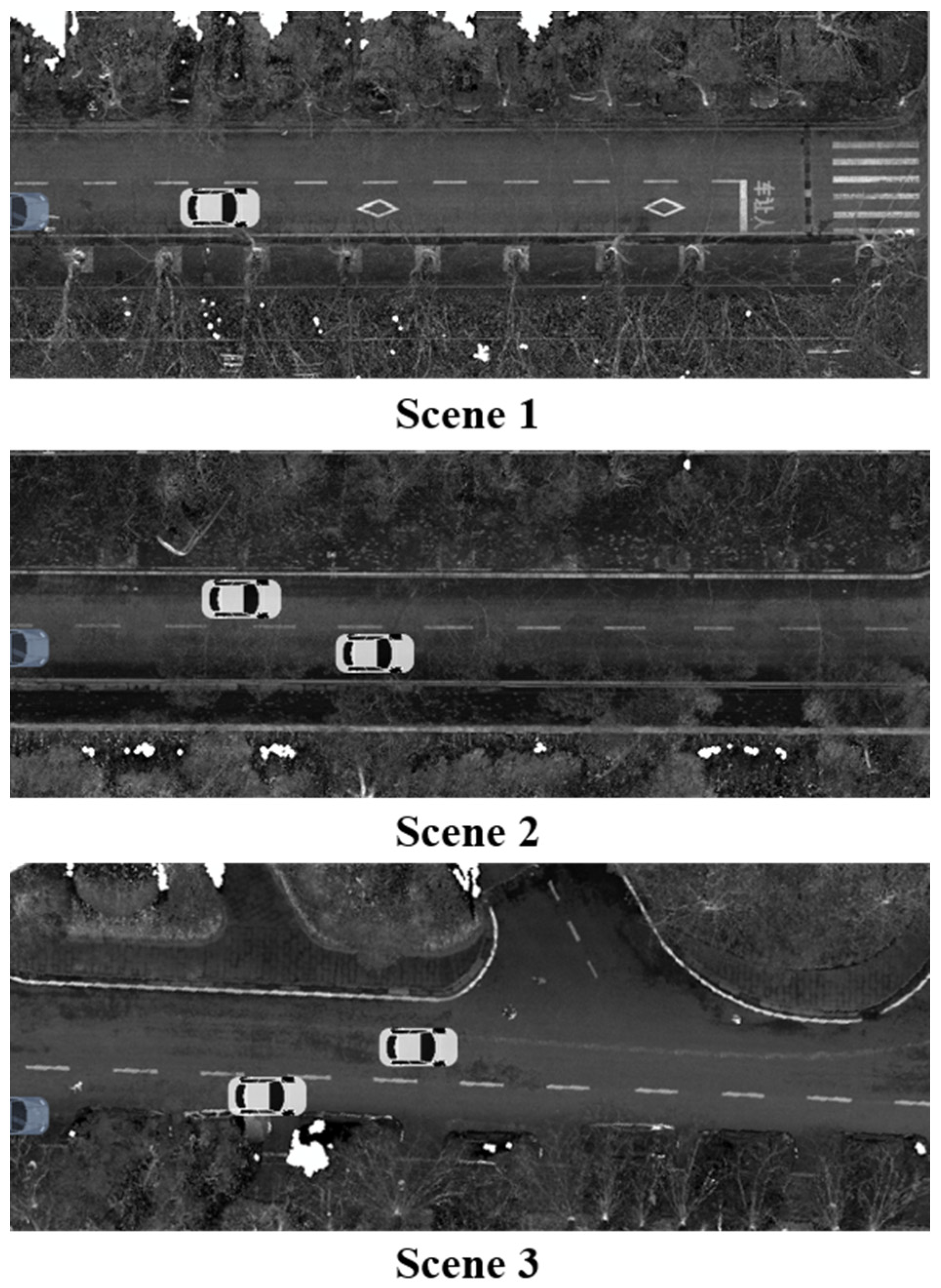
5.1.2. Experimental Environment

We chose a campus road in Wuhan University as the experimental environment, as shown in Figure 13. Figure 13a shows the HD-Map of Wuhan University, and Figure 13b shows a vector map of our experimental environment. The main driving parameters of the road in this experimental environment are shown in Table 4.
The environment has a variety of traffic participants such as moving vehicles, electric bicycles, pedestrians and static obstacles. The traffic rules on campus are less restrictive; for example, pedestrians and bicycles do not necessarily cross the street using the sidewalks, and vehicles may stop at the side of the road. There are two intersections, six T-junctions and several irregular roads. The speed limit on campus is 30 km/h; therefore, our AV drove at medium and low speed in the experiment, with a speed of less than 30 km/s. The roads in our experiments were all two-lane, with lane widths between 2.3 and 3 m.

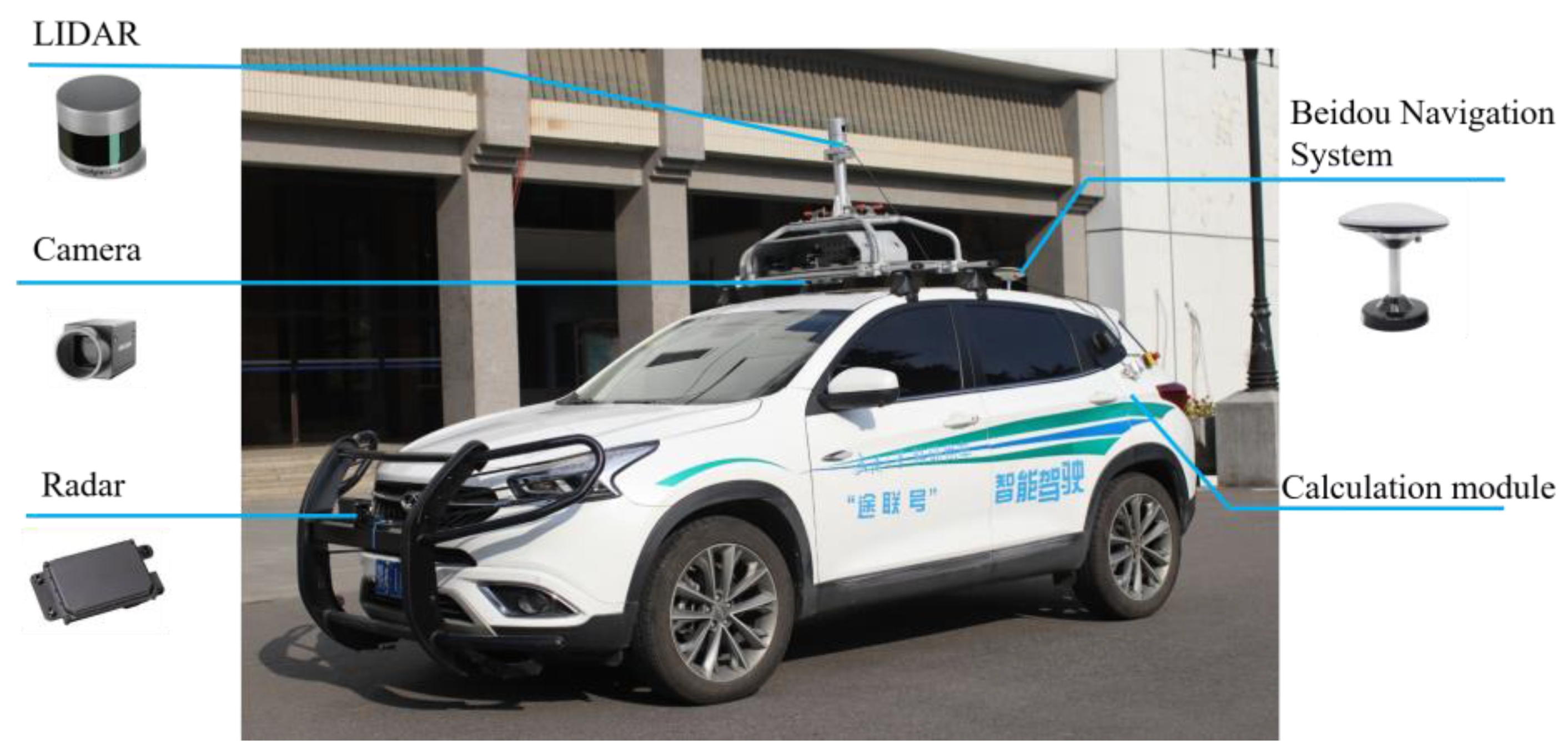
5.1.3. Experimental Platform

We used the AV independently developed by the 3 S team of the State Key Laboratory of Information Engineering in Surveying, Mapping, and Remote Sensing of Wuhan University to conduct the experiments. Our experimental AV is shown in Figure 14, the main sensors and configurations on it are shown in Table 5, and programming languages, platforms and visualizations used for the three experiments are shown in Table 6.
Our AV is 4.3 m long, 1.7 m wide and 2.2 m high (with sensors). The sensors used on our experimental vehicle include a LIDAR, millimeter-wave radars, cameras and navigation systems. We used a navigation system that integrates inertial navigation, Beidou satellite navigation and a wheel speedometer. The 32-line LIDAR is on the top of the AV, and the millimeter-wave radars are on the front and rear of the AV. Four cameras, including a depth camera, are positioned on the front of the car.

5.1.4. Experimental Steps

In order to achieve the above experimental objectives, we designed the following experimental steps:
Step 1: The campus road of Wuhan University was selected as the experimental environment, and the HD-Map data and perceptual layer data were processed in advance.
Step 2: The sensors such as IMU, GNSS and LIDAR on the AV were calibrated first. Then, the AV was driven to the specified location to conduct the sampling experiment of the three sampling strategies, namely, random distribution sampling, Gaussian distribution sampling and the proposed CR-Map and Gaussian combination sampling.
Step 3: RRT*, DT-RRT* and the proposed algorithm were run on the AV in three typical scenes for 100 times. The number of iterations, the number of nodes and the number of trajectories of each algorithm were counted and compared.
Step 4: The four motion planning algorithms mentioned were run on campus, and the computation time of each algorithm was counted to analyze the algorithmic efficiency.

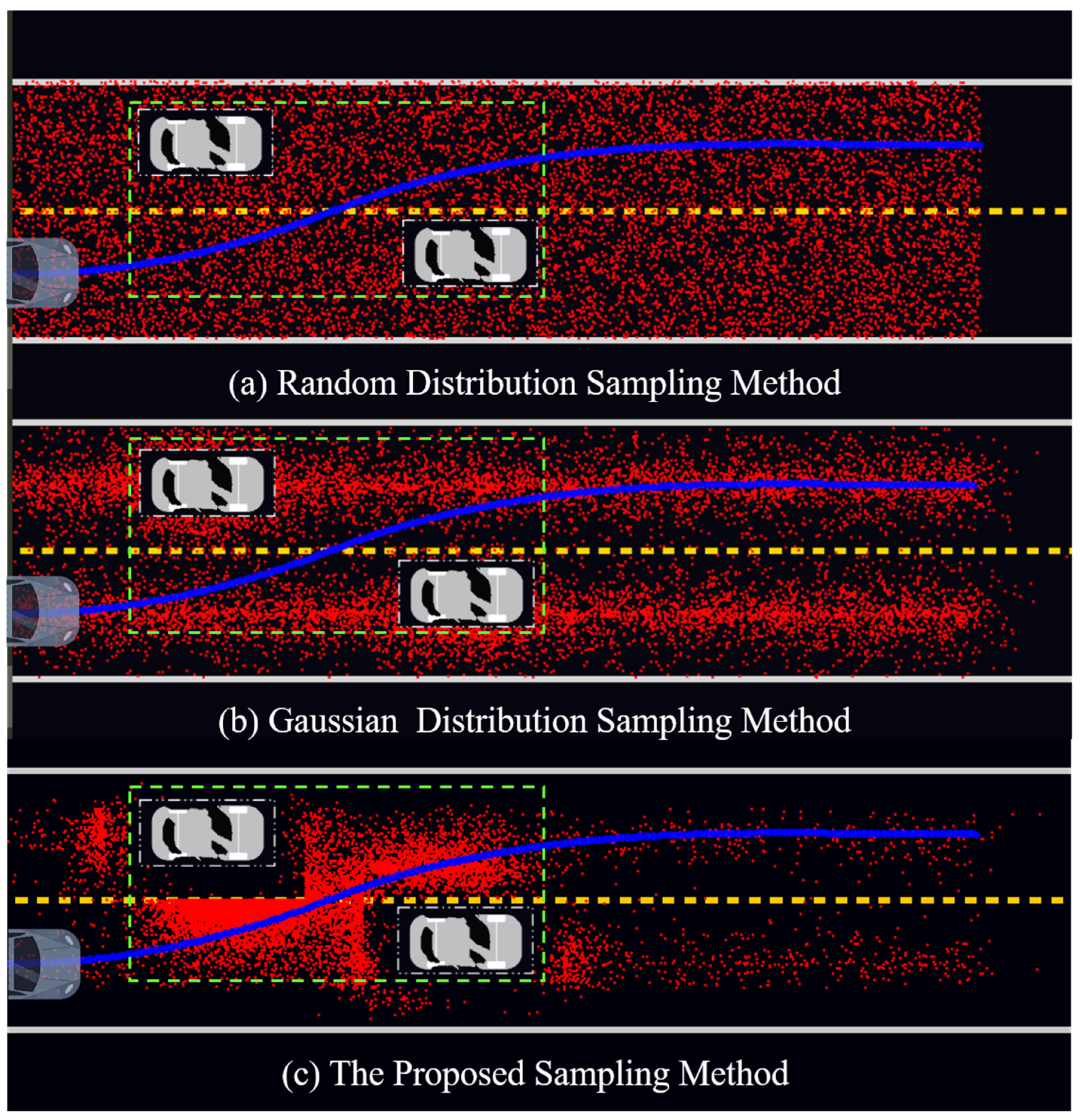
5.2. Sampling Efficiency Analysis

We selected a typical scene to conduct the sampling experiment. The random distribution sampling, the Gaussian distribution sampling and the proposed CR-Map and Gaussian combination sampling method were run to generate 10,000 samples in this scenario, and the results are shown in Figure 15.
This scenario has two lanes in the same direction, separated by a dashed yellow line. In Figure 15, the blue vehicle represents the starting position of the AV, the white vehicles are stationary obstacles, the red points are the sampling points and the blue curve is the optimal trajectory. The area around the obstacles is our area of interest (AOI), which is the green dotted box area. In sampling-based motion planning algorithms, avoiding obstacles is the key process. When the sampling points are concentrated around the obstacles, the feasible trajectory can be obtained faster, and the iteration times of the algorithm can be reduced. Figure 15a shows that the sampling points obtained by the random distribution sampling method are uniformly distributed in the configuration space. This random approach is very inefficient. The points sampled using the Gaussian method in Figure 15b are distributed near the center line of the two lanes, but there are few points in the obstacle area. Different from the two methods, the proposed sampling method in Figure 15c significantly increases the number of samples in the key area near the obstacles. This is achieved by increasing the probability of sampling in the gradient descent regions on the CR-Map. The CR-Map is a grid map reflecting the collision risk coefficient on the road, and the gradient descent regions cover the surrounding areas of the obstacles.
In this paper, two indexes are set up to evaluate the sampling efficiency. One is the probability that the sampling points fall in the obstacle intersection area (AOI, green box), and the other is the probability that the sampling points fall near the optimal trajectory (blue curve). Table 7 shows the sampling efficiency analysis results of the three methods.
As can be seen in Table 7, the probability that the sampling points obtained using the proposed method fall in the AOI is 8013/10,000, which is much higher than that of the other two methods. The probability that the sampling points of the proposed method fall near the optimal trajectory is 3648/10,000, which is also significantly higher than that of the other two methods. The higher the probability that the sampling point falls in the area of interest, the fewer iterations needed to pass the obstacle. The number of iterations required for the three different algorithms will be analyzed in the node optimization experiment in the next section.

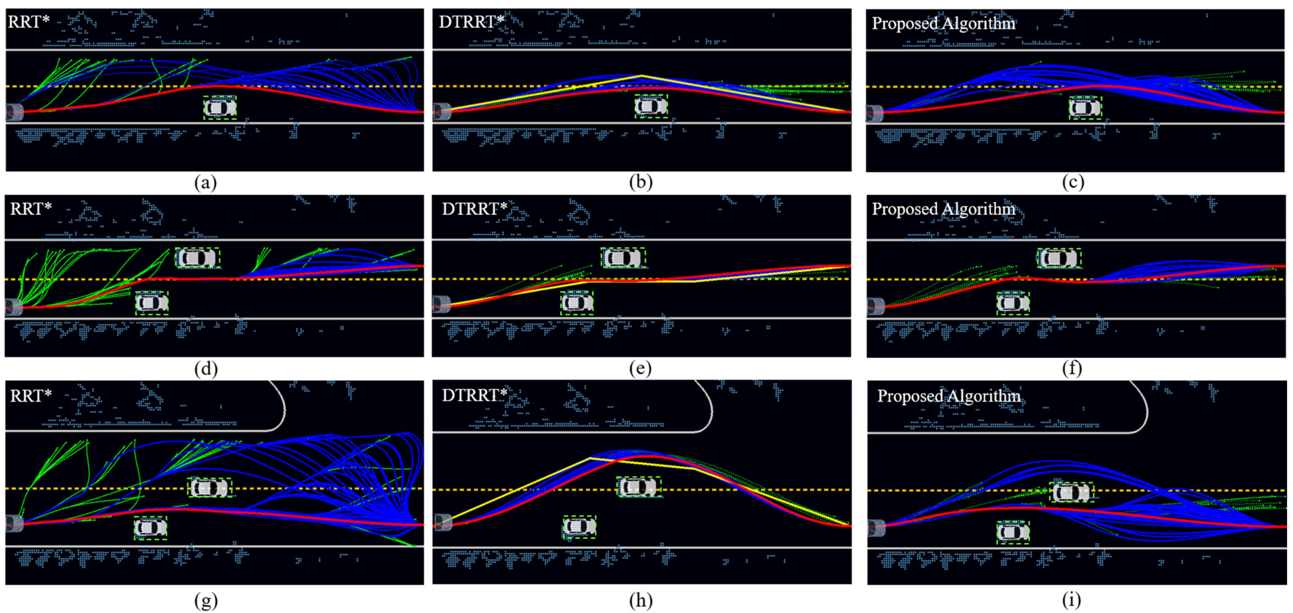
5.3. Node Optimization Analysis

We set up three typical scenes to carry out the node optimization experiments of the three algorithms: RRT*, DT-RRT* and the proposed algorithm. For the sake of experimental rigor, we used the same vehicle kinematic model and collision detection methods in the three algorithms. In addition, a fast clothoid fitting method was used to compute the steering procedure. The RRT* [19] algorithm uses the original framework described in Algorithm 1 and a Gaussian distribution sampling method. The DT-RRT* [21] algorithm proposed by Chen and Shan was also from our team. It uses a double-tree structure to improve the efficiency of the algorithm. The proposed algorithm uses the novel algorithm framework and the CR-Map and Gaussian combination sampling introduced in Section 4.2. The three experimental scenes are all on the campus road of Wuhan University, as shown in Figure 16.
Scene 1 is a simple lane-changing overtaking scenario. Scene 2 is a narrow corridor formed by two obstacles, with a longitudinal distance of less than 4 m and horizontal distances of less than 1 m. This scenario requires the AV to drive a smooth curve to avoid obstacles along the way, which is used to verify the abilities of the algorithms in narrow corridors. Scene 3 is a trapping experiment with two completely different solutions. One is wide and easy to find, but over a longer distance. The other is narrow and difficult to find, but over a shorter distance. This scene can be used to verify whether the algorithm can jump out of the trap and find an optimal solution. Each algorithm was run 100 times in three scenarios to analyze the node optimization efficiency. The results are shown in Figure 17.
In each result of Figure 17, the light-blue car on the left represents the starting position of the vehicle, the white vehicles represent the obstacles and the direction is from left to right. The green curves are the tree, the blue curves are the trajectories and the red curves are the optimal trajectories. In Figure 17b,e,h, the yellow polylines are the reference trajectories generated using the DT-RRT algorithm. The light-blue points outside the road boundary are the projection points of the LIDAR point cloud.
From Figure 17, we can see that the tree of the DT-RRT* algorithm and the proposed algorithm is more convergent and concentrated than that of the RRT* algorithm. The DT-RRT* algorithm has the most concentrated tree, because it calculates the reference trajectory first and then the samples near the reference trajectory (the yellow polyline). The convergence rate can be improved in this way, but the feasible trajectories cannot jump out of the range of the reference trajectory. Therefore, in Figure 17h, there is a certain probability that the DT-RRT* algorithm cannot get out of the trap and can only find the suboptimal trajectories. When the reference trajectory obtained by the first tree of the DT-RRT* algorithm is non-optimal, the whole algorithm cannot find the optimal solution. Different from the DT-RRT* algorithm, the proposed algorithm can not only improve the convergence rate but also ensure the exploratory and optimal solution. Next, we will analyze the node optimization efficiency of the three algorithms from the perspective of statistical data, as shown in Table 8.
In Table 8, four indexes are set up to evaluate the node optimization efficiency, which are the iterations of the first trajectory, the iterations of the optimal trajectory, the frequency of failures and the length of the optimal trajectory. In each column, the statistical results of the three scenarios are arranged from top to bottom. It can be seen in Table 8 that the number of iterations of the proposed algorithm to obtain the first trajectory and the optimal trajectory in the three scenarios is significantly smaller than that of the other two algorithms, and the optimal trajectory length obtained by the proposed algorithm is basically the shortest. This indicates that the convergence rate of our approach is faster than the existing two algorithms while ensuring the trajectory quality. The performance of the three algorithms in different scenarios is described in detail below.
Scene 1 is a simple lane-changing overtaking scenario. The average number of iterations of the first trajectory of the proposed method is nine, which is much lower than the fifty-two and forty-one iterations of the RRT* and DT-RRT* algorithms. This shows that the proposed algorithm finds the feasible trajectory much faster than the existing method. For the iterations of the optimal trajectory, the proposed algorithm also significantly outperforms the other two algorithms. Our approach’s convergence rate to the optimal solution is about 3 times faster than RRT* and 1.5 times faster than DT-RRT* in scene 1. The DT-RRT* algorithm needs a large number of iterations even if its tree converges, because its reference trajectory also needs to be obtained by sampling. The optimal trajectory length obtained by the three algorithms is similar.
In Scene 2, there is a narrow corridor where feasible trajectories are more difficult to find. Therefore, the three algorithms require more iterations than Scene 1. Similar to Scene 1, the proposed algorithm requires less iterations to obtain the first feasible trajectory and the optimal trajectory than the other two algorithms. As can be seen in Figure 17d, the tree of the original RRT* algorithm is very divergent, and it takes, on average, 259 iterations to find a feasible trajectory. Moreover, the original RRT* algorithm fails to find a feasible trajectory 11 times out of 100. The DT-RRT* algorithm also takes an average of 108 iterations to find the first feasible trajectory, while the proposed algorithm only takes an average of 24 iterations to find the first feasible trajectory. In summary, our proposed method converges about 3 times faster than RRT* and 1.7 times faster than DT-RRT* in scene 2. It is achieved by the heuristic information provided via the CR-Map, which can improve the sampling and node optimization efficiency of the proposed algorithm and greatly accelerate the convergence rate.
Scene 3 is a trap experiment, with a longer path that is easy to find, and a shorter path that is less easy to find. As can be seen in Figure 17g–i, both the original RRT* and the proposed algorithm jump out of the trap and find the optimal trajectory, but the DT-RRT algorithm fails to jump out of the trap. Because the reference trajectory obtained using DT-RRT* through the first tree fails to find the optimal solution, the whole algorithm is affected. Because the proposed algorithm preferentially samples in the gradient descent region in the CR-Map, it is easier for it to find the corridor between the two obstacles. At the same time, by optimizing the cost function of finding the optimal parent node, it is easier for the algorithm to converge to the solution with the minimum comprehensive cost. In Scene 3, the convergence rate of our approach is about 4 times faster than RRT* and slightly faster than DT-RRT*.
Through the node optimization experiment, the proposed algorithm can improve the convergence rate while ensuring the trajectory quality and strong exploration. The convergence rate of the proposed algorithm in the three scenes are significantly faster than the other two existing algorithms. In the next section, we will collect the computation time of the three algorithms and analyze their algorithmic efficiency by conducting an autonomous driving experiment without intervention.

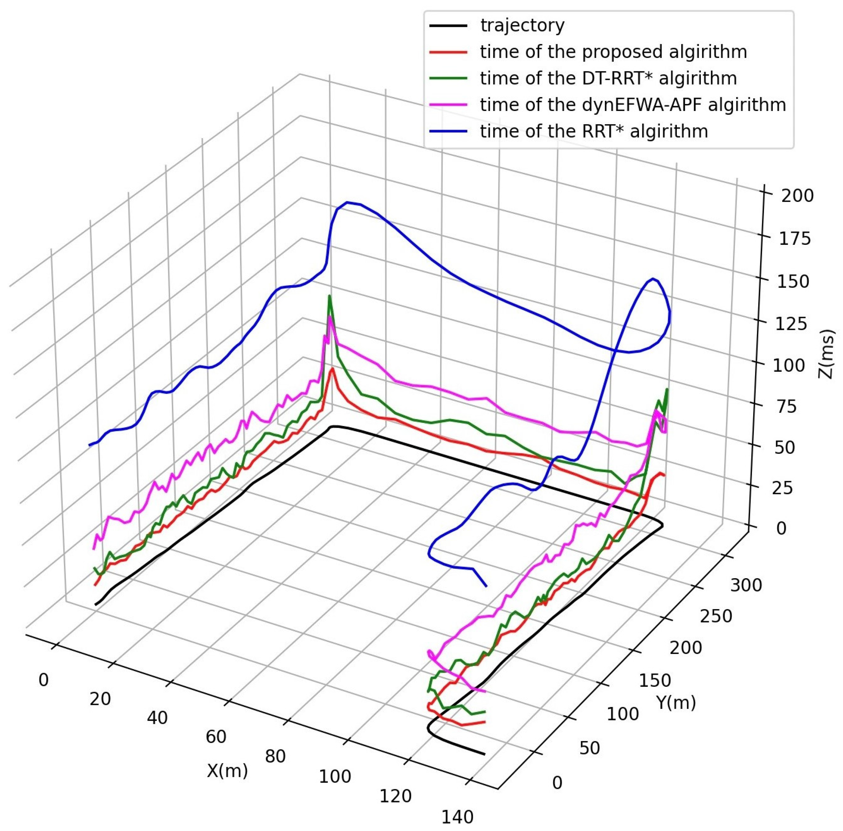
5.4. Algorithm Efficiency Analysis

We selected the road in Wuhan University to conduct the autonomous driving experiments without human intervention, in order to analyze the algorithmic efficiency of the four motion planning methods. The body of our algorithm was written in C++, using a computing module installed in our AV. The experiment scene is shown in Figure 18.
Figure 18a shows the experimental environment of the algorithm efficiency experiment, the purple part of Figure 18b is the vector layer of the map and the blue points are the trajectory of this experiment. The trajectory is about one kilometer long, with one intersection and three T-junctions. Several sensors were used including a map module, integrated navigation system, LIDAR module, vision module and the AV’s control system. In the motion planning system, the re-planning command would be triggered when the planned trajectory encounters obstacles, drives to the re-planning point or decides to change the trajectory. We set a motion planning process from the beginning to obtain the first feasible trajectory as one full-cycle re-planning process. Table 9 shows the statistical data of each planning after each algorithm completed the experiment.
As can be seen from the results in Table 9, the RRT* algorithm failed four times, and the dynEFWA-APF algorithm failed once. The proposed algorithm and DT-RRT* algorithm have no manual intervention for planning failure. The RRT* algorithm failed at the same intersection where the right-turn road was narrowed due to construction. After four manual adjustments to the vehicle’s position, the RRT* algorithm passed successfully. The dynEFWA-APF algorithm failed between the playground gate and the T-junction. The algorithm picked a road into the playground that cannot be backed out of. After manual intervention to adjust the position of the vehicle, the algorithm successfully passed. Since the dynEFWA-APF algorithm is not a sampling-based algorithm and does not need to throw sampling points to explore the environment, the indexes of average iterations of first trajectory and average iterations of optimal trajectory are not evaluated.
In Table 9, the average number of iterations of the proposed algorithm on the first trajectory is about nine times less than RRT* and three times less than DT-RRT*. The average number of iterations of the proposed algorithm on the optimal trajectory is about four times less than RRT* and slightly less than DT-RRT*. It means that the convergence rate of our approach is faster than the RRT* and DT-RRT*, which is consistent with the conclusion in the node optimization experiment. In terms of the number of feasible trajectories obtained, the proposed algorithm also obtains more trajectories than the RRT* and DT-RRT* algorithms. Because the sampling points of the proposed algorithm are concentrated in the AOI, more effective nodes and trajectories can be obtained in the same number of iterations. The average computation time of RRT*, DT-RRT*, dynEFWA-APF and the proposed algorithm is 104.79 ms, 24.10 ms, 42.24 ms and 15.98 ms, respectively. It means that the proposed algorithm also outperforms the other three algorithms in terms of the computational time to obtain the first feasible trajectory. The computation time consumed by each re-planning of the four algorithms in this experiment is shown in Figure 19.
In Figure 19, the brown curve in the XY plane is the driving trajectory of this experiment. The coordinates of the X and Y axes are in meters. The Z axis is in milliseconds, representing the computation time. A larger value of Z indicates that the algorithm is more time-consuming and less efficient. The blue curve is the time of the RRT* algorithm, the green curve is the time of the DT-RRT* algorithm, the pink curve is the time of the dynEFWA-APF algorithm and the red curve is the time of the proposed algorithm. As can be seen in Figure 19, the RRT* algorithm has the longest re-planning time, followed by the DT-RRT* algorithm, and the proposed algorithm has the shortest re-planning time. The computational time of the proposed algorithm is within 20 ms, that of the DT-RRT* algorithm is also around 20 ms, that of the dynEFWA-APF algorithm is around 40 ms and that of the original RRT* algorithm is around 100 ms. When it comes to the intersection, the computational time of the four motion planning algorithms increases considerably. The computation time of DT-RRT* at the intersection reaches 90 ms, and that of the original RRT* algorithm reaches 150 ms. However, the proposed algorithm can still calculate the first feasible trajectory within 30 ms at the intersection. The reason why the proposed algorithm requires the least computation time will be analyzed next.
The original RRT* algorithm needs to adjust the structure of the tree for each rewire process of the iteration, which results in it having the longest computation time. The DT-RRT* algorithm can ensure high computational efficiency, but the calculation time will rise sharply at the intersection. Because DT-RRT* is a double-tree algorithm, its performance depends on the reference path generated via the first RRT tree. When the environment becomes complicated, such as the intersection, the time for the RRT tree to find the optimal trajectory becomes longer, or it cannot even find the optimal solution. The calculation time of the dynEFWA-APF algorithm is relatively stable because it is not a random sampling algorithm. Its computation time is limited by the complexity of the environment. The proposed algorithm has the shortest computation time and can deal with the intersections well, because the proposed algorithm combines the prior information of the HD-Map and the fast exploration of the RRT algorithm. At the intersections, due to the guidance of the HD-Map, the sampling points are concentrated in the effective areas, which greatly reduces the planning time. After the first feasible trajectory is obtained, the proposed algorithm will continue sampling to continuously optimize the trajectory until the next re-planning. This experiment shows that the proposed algorithm outperforms the original RRT* algorithm, dynEFWA-APF algorithm and DT-RRT* algorithm in terms of algorithm efficiency.
In general, through sampling efficiency experiments, node optimization experiments and algorithm efficiency experiments, it can be seen that the proposed algorithm optimizes the sampling efficiency, accelerates the convergence speed, reduces the number of iterations and improves the algorithm efficiency. Moreover, the proposed algorithm can meet the real-time requirements of autonomous driving in the complex campus environment while ensuring the trajectory quality.

6. Conclusions

In this paper, we proposed a fast HD-Map-guided motion planning algorithm, HDM-RRT, to solve the autonomous driving problem in challenging campus environments. One of the innovations is that we propose a CR-Map that quantifies the collision risk coefficient on the road and combines it with the Gaussian distribution for sampling. Results of experiments show that the sampling efficiency of our proposed method is four times higher than that of Gaussian distribution sampling. Then, we deeply optimize the node optimization strategy through the prior information of the CR-Map. It improves the convergence rate of the algorithm and is beneficial to the stability of AVs in campus environments. In real scenario experiments, the average computation time of the proposed algorithm is only 15.98 ms, which is much better than that of the three compared algorithms. It illustrates that our approach is competent for autonomous driving in campus environments and has significant implications for campus applications such as self-driving buses, autonomous logistics and unmanned patrol vehicles. However, further improvements can also be made to the proposed algorithm. A possible direction is to continue optimizing sampling methods to accommodate different road scenarios, such as intersections and U-turn scenarios. Another direction is to continue mining HD-Map information to generate not only collision risk maps but also safe driving areas to guide AVs.

Author Contributions

X.G. made contributions to the research conception, experimental design and manuscript writing; Y.C. helped with the design and analysis of the experiments; J.Z. gave instructions for the graphs, tables and structure of the paper; Y.H. contributed to the processing of perception and map data; B.L. gave guidance to the conception and experimental design of the paper. All authors have read and agreed to the published version of the manuscript.

Funding

This work was supported by the National Key Research and Development Program of China under Grant 2021YFB2501100.

Data Availability Statement

The data that support the findings of this study are available from the corresponding author upon reasonable request.

Conflicts of Interest

The authors declare no conflict of interest.

References

  1. Schwarting, W.; Alonso-Mora, J.; Rus, D. Planning and decision-making for autonomous vehicles. Annu. Rev. Control. Robot. Auton. Syst. 2018, 1, 187–210. [Google Scholar] [CrossRef]
  2. Pei, S.; Kretzschmar, H.; Dotiwalla, X.; Chouard, A.; Patnaik, V.; Tsui, P.; Guo, J.; Zhou, Y.; Chai, Y.; Caine, B.; et al. Scalability in perception for autonomous driving: Waymo open dataset. In Proceedings of the IEEE/CVF Conference on Computer Vision and Pattern Recognition (CVPR), Seattle, WA, USA, 10 December 2019; pp. 2443–2451. [Google Scholar]
  3. Levinson, J.; Askeland, J.; Becker, J.; Dolson, J.; Held, D.; Kammel, S.; Kolter, J.Z.; Langer, D.; Pink, O.; Pratt, V.; et al. Towards fully autonomous driving: Systems and algorithms. In Proceedings of the 2011 IEEE Intelligent Vehicles Symposium (IV), New York, NY, USA, 5–9 June 2011; pp. 163–168. [Google Scholar]
  4. Zhou, J.; Guo, Y.; Bian, Y.; Huang, Y.; Li, B. Lane Information Extraction for High Definition Maps Using Crowdsourced Data. IEEE Trans. Intell. Transp. Syst. 2022, 1–11. [Google Scholar] [CrossRef]
  5. Aldibaja, M.; Suganuma, N.; Yanase, R. 2.5D Layered Sub-Image LIDAR Maps for Autonomous Driving in Multilevel Environments. Remote Sensing 2022, 14, 5847. [Google Scholar] [CrossRef]
  6. Xiao, J.; Guo, H.; Yao, Y.; Zhang, S.; Zhou, J.; Jiang, Z. Multi-Scale Object Detection with the Pixel Attention Mechanism in a Complex Background. Remote Sens. 2022, 14, 3969. [Google Scholar] [CrossRef]
  7. Zhang, H.; Li, W.; Qian, C.; Li, B. A real time localization system for vehicles using terrain-based time series subsequence matching. Remote Sens. 2020, 12, 2607. [Google Scholar] [CrossRef]
  8. Kang, M.-S.; Ahn, J.-H.; Im, J.-U.; Won, J.-H. Lidar- and V2X-Based Cooperative Localization Technique for Autonomous Driving in a GNSS-Denied Environment. Remote Sens. 2022, 14, 5881. [Google Scholar] [CrossRef]
  9. Shan, Y.; Zheng, B.; Chen, L.; Chen, L.; Chen, D. A reinforcement learning-based adaptive path tracking approach for autonomous driving. IEEE Trans. Veh. Technol. 2020, 69, 10581–10595. [Google Scholar] [CrossRef]
  10. Feng, G.; Han, Y.; Li, S.E.; Shaobing, X.; Dongfang, D. Accurate Pseudospectral Optimization of Nonlinear Model Predictive Control for High-performance Motion Planning. IEEE Trans. Intell. Veh. 2022, 1. [Google Scholar] [CrossRef]
  11. Latombe, J.C. Motion planning: A journey of robots, molecules, digital actors, and other artifacts. Int. J. Robot. Res. 1999, 18, 1119–1128. [Google Scholar] [CrossRef]
  12. Li, B.; Liu, S.; Tang, J.; Gaudiot, J.L.; Zhang, L.; Kong, Q. Autonomous last-mile delivery vehicles in complex traffic environments. Computer 2020, 53, 26–35. [Google Scholar] [CrossRef]
  13. Wu, Y.; Ding, Y.; Ding, S.; Savaria, Y.; Li, M. Autonomous Last-Mile Delivery Based on the Cooperation of Multiple Heterogeneous Unmanned Ground Vehicles. Math. Probl. Eng. 2021, 2021, 5546581. [Google Scholar] [CrossRef]
  14. Wang, H.; Zhang, L.; Kong, Q.; Zhu, W.; Zheng, J.; Zhuang, L.; Xu, X. Motion planning in complex urban environments: An industrial application on autonomous last-mile delivery vehicles. J. Field Robot. 2022, 39, 1258–1285. [Google Scholar] [CrossRef]
  15. Dolgov, D.; Thrun, S.; Montemerlo, M.; Diebel, J. Path planning for autonomous vehicles in unknown semi-structured environments. Int. J. Robot. Res. 2010, 29, 485–501. [Google Scholar] [CrossRef]
  16. Karur, K.; Sharma, N.; Dharmatti, C.; Siegel, J.E. A survey of path planning algorithms for mobile robots. Vehicles 2021, 3, 448–468. [Google Scholar] [CrossRef]
  17. Paden, B.; Čáp, M.; Yong, S.Z.; Yershov, D.; Frazzoli, E. A survey of motion planning and control techniques for self-driving urban vehicles. IEEE Trans. Intell. Veh. 2016, 1, 33–55. [Google Scholar] [CrossRef] [Green Version]
  18. LaValle, S.M. Rapidly-Exploring Random Trees: A New Tool for Path Planning; TR 98-11; Department of Computer Science, Iowa State University: Ames, IA, USA, 1998. [Google Scholar]
  19. Karaman, S.; Frazzoli, E. Sampling-based algorithms for optimal motion planning. Int. J. Robot. Res. 2011, 30, 846–894. [Google Scholar] [CrossRef] [Green Version]
  20. Wang, J.; Li, B.; Meng, M.Q.H. Kinematic Constrained Bi-directional RRT with Efficient Branch Pruning for robot path planning. Expert Syst. Appl. 2021, 170, 114541. [Google Scholar] [CrossRef]
  21. Chen, L.; Shan, Y.; Tian, W.; Li, B.; Cao, D. A fast and efficient double-tree RRT-like sampling-based planner applying on mobile robotic systems. IEEE/ASME Trans. Mechatron. 2018, 23, 2568–2578. [Google Scholar] [CrossRef]
  22. Zheng, L.; Song, H.; Li, B.; Zhang, H. Generation of lane-level road networks based on a trajectory-similarity-join pruning strategy. ISPRS Int. J. Geo.-Inf. 2019, 8, 416. [Google Scholar] [CrossRef] [Green Version]
  23. Zuo, X.; Zhou, J.; Yang, F.; Su, F.; Zhu, H.; Li, L. Real-time Global Action Planning for Unmanned Ground Vehicle Exploration in Three-dimensional Spaces. Expert Syst. Appl. 2022, 215, 119264. [Google Scholar] [CrossRef]
  24. Dijkstra, E.W. A note on two problems in connexion with graphs. Numer. Math. 1959, 1, 269–271. [Google Scholar] [CrossRef] [Green Version]
  25. Hart, P.E.; Nilsson, N.J.; Raphael, B. A formal basis for the heuristic determination of minimum cost paths. IEEE Trans. Syst. Sci. Cybern. 1968, 4, 100–107. [Google Scholar] [CrossRef]
  26. Kathib, O. Real-time obstacle avoidance for manipulators and mobile robots. Int. J. Robot. Res. 1986, 5, 490–496. [Google Scholar]
  27. Min, H.; Xiong, X.; Wang, P.; Yu, Y. Autonomous driving path planning algorithm based on improved A algorithm in unstructured environment. Proc. Inst. Mech. Eng. Part D J. Automob. Eng. 2021, 235, 513–526. [Google Scholar] [CrossRef]
  28. Tang, G.; Tang, C.; Claramunt, C.; Hu, X.; Zhou, P. Geometric A-star algorithm. An improved A-star algorithm for AGV path planning in a port environment. IEEE Access 2021, 9, 59196–59210. [Google Scholar] [CrossRef]
  29. Dolgov, D.; Thrun, S.; Montemerlo, M.; Diebel, J. Practical search techniques in path planning for autonomous driving. Ann. Arbor. 2008, 1001, 18–80. [Google Scholar]
  30. Koren, Y.; Borenstein, J. Potential field methods and their inherent limitations for mobile robot navigation. Icra 1991, 1398–1404. [Google Scholar]
  31. Xinyu, W.; Xiaojuan, L.; Yong, G.; Jiadong, S.; Rui, W. Bidirectional potential guided rrt for motion planning. IEEE Access 2019, 7, 95046–95057. [Google Scholar] [CrossRef]
  32. Wang, P.; Gao, S.; Li, L.; Sun, B.; Cheng, S. Obstacle avoidance path planning design for autonomous driving vehicles based on an improved artificial potential field algorithm. Energies 2019, 12, 2342. [Google Scholar] [CrossRef] [Green Version]
  33. Li, H.; Liu, W.; Yang, C.; Wang, W.; Qie, T.; Xiang, T. An Optimization-based Path Planning Approach for Autonomous Vehicles using dynEFWA-Artificial Potential Field. IEEE Trans. Intell. Veh. 2021, 7, 263–272. [Google Scholar] [CrossRef]
  34. LaValle, S.M.; Kuffner Jr, J.J. Randomized kinodynamic planning. Int. J. Robot. Res. 2001, 20, 378–400. [Google Scholar] [CrossRef]
  35. Kuwata, Y.; Teo, J.; Fiore, G.; Karaman, S.; Frazzoli, E.; How, J.P. Real-time motion planning with applications to autonomous urban driving. IEEE Trans. Control Syst. Technol. 2009, 17, 1105–1118. [Google Scholar] [CrossRef]
  36. Jaillet, L.; Hoffman, J.; Van den Berg, J.; Abbeel, P.; Porta, J.M.; Goldberg, K. EG-RRT: Environment-guided random trees for kinodynamic motion planning with uncertainty and obstacles. In Proceedings of the International Conference on Intelligent Robots and Systems, San Francisco, CA, USA, 25–30 September 2011; pp. 2646–2652. [Google Scholar]
  37. Perez, A.; Platt, R.; Konidaris, G.; Kaelbling, L.; Lozano-Perez, T. LQR-RRT: Optimal sampling-based motion planning with automatically derived extension heuristics. In Proceedings of the 2012 IEEE International Conference on Robotics and Automation, St Paul, MN, USA, 14–18 May 2012; pp. 2537–2542. [Google Scholar]
  38. Karaman, S.; Frazzoli, E. Incremental sampling-based algorithms for optimal motion planning. Robot. Sci. Syst. VI 2010, 104. [Google Scholar] [CrossRef]
  39. Gammell, J.D.; Strub, M.P. Asymptotically optimal sampling-based motion planning methods. Annu. Rev. Control. Robot. Auton. Syst. 2021, 4, 295–318. [Google Scholar] [CrossRef]
  40. Salzman, O.; Halperin, D. Asymptotically near-optimal RRT for fast, high-quality motion planning. IEEE Trans. Robot. 2016, 32, 473–483. [Google Scholar] [CrossRef] [Green Version]
  41. Littlefield, Z.; Bekris, K.E. Informed asymptotically near-optimal planning for field robots with dynamics. In Field and Service Robotics; Springer: Cham, Switzerland, 2018; pp. 449–463. [Google Scholar]
  42. Pareekutty, N.; James, F.; Ravindran, B.; Shah, S.V. qRRT: Quality-Biased Incremental RRT for Optimal Motion Planning in Non-Holonomic Systems. arXiv 2021, arXiv:2101.02635, 2021. [Google Scholar]
  43. Gan, Y.; Zhang, B.; Ke, C.; Zhu, X.; He, W.; Ihara, T. Research on Robot Motion Planning Based on RRT Algorithm with Nonholonomic Constraints. Neural Process. Lett. 2021, 53, 3011–3029. [Google Scholar] [CrossRef]
  44. Yuncheng, L.; Jie, S. A revised Gaussian distribution sampling scheme based on RRT algorithms in robot motion planning. In Proceedings of the 2017 3rd International Conference on Control, Automation and Robotics (ICCAR), Nagoya, Japan, 24–26 April 2017; pp. 22–26. [Google Scholar]
  45. Xi, H. Obstacle avoidance trajectory planning of redundant robots based on improved Bi-RRT. Int. J. Syst. Assur. Eng. Manag. 2021, 1–10. [Google Scholar] [CrossRef]
  46. Ge, Q.; Li, A.; Li, S.; Du, H.; Huang, X.; Niu, C. Improved Bidirectional RRT Path Planning Method for Smart Vehicle. Math. Probl. Eng. 2021, 2021, 6669728. [Google Scholar] [CrossRef]
  47. Qureshi, A.H.; Iqbal, K.F.; Qamar, S.M.; Islam, F.; Ayaz, Y.; Muhammad, N. Potential guided directional-RRT for accelerated motion planning in cluttered environments. In Proceedings of the 2013 IEEE International Conference on Mechatronics and Automation, Takamatsu, Japan, 4–7 August 2013; pp. 519–524. [Google Scholar]
  48. Tang, X.; Chen, F. Robot path planning algorithm based on bi-rrt and potential field. In Proceedings of the 2020 IEEE International Conference on Mechatronics and Automation (ICMA), Beijing, China, 13–16 October 2020; pp. 1251–1256. [Google Scholar]
  49. An, H.; Hu, J.; Lou, P. Obstacle Avoidance Path Planning Based on Improved APF and RRT. In Proceedings of the 2021 4th International Conference on Advanced Electronic Materials, Computers and Software Engineering (AEMCSE), Changsha, China, 26–28 March 2021; pp. 1028–1032. [Google Scholar]
  50. Polack, P.; Altché, F.; d’Andréa-Novel, B.; de La Fortelle, A. The kinematic bicycle model: A consistent model for planning feasible trajectories for autonomous vehicles? In Proceedings of the 2017 IEEE Intelligent Vehicles Symposium (IV), Los Angeles, CA, USA, 11–14 June 2017; pp. 812–818. [Google Scholar]
  51. Bertolazzi, E.; Frego, M. Fast and accurate clothoid fitting. arXiv 2012, arXiv:1209.0910. [Google Scholar]
  52. Shan, Y.; Yang, W.; Chen, C.; Zhou, J.; Zheng, L.; Li, B. CF-pursuit: A pursuit method with a clothoid fitting and a fuzzy controller for autonomous vehicles. Int. J. Adv. Robot. Syst. 2015, 12, 134. [Google Scholar] [CrossRef]
Figure 1. Examples of Wuhan University campus scenes (a,b).
Remotesensing 15 00487 g001
Figure 2. Overall architecture of the algorithm (ad).
Remotesensing 15 00487 g002
Figure 3. The HD-Map information of three campus scenes (ac).
Remotesensing 15 00487 g003
Figure 4. Kinematic model of an autonomous vehicle.
Remotesensing 15 00487 g004
Figure 5. An example of a CR-Map (a,b).
Remotesensing 15 00487 g005
Figure 6. Random distribution sampling.
Remotesensing 15 00487 g006
Figure 7. Gaussian distribution sampling.
Remotesensing 15 00487 g007
Figure 8. Road environment containing obstacles.
Remotesensing 15 00487 g008
Figure 9. The combined CR-Map and Gaussian distribution sampling.
Remotesensing 15 00487 g009
Figure 10. New rewire process of HDM-RRT, where (a) is the initial state, (b) is the collision and kinematic limitation, (c) shows the selection of the optimal parent node using the cost function and (d) shows the tracing of the parent node to the starting point to find out whether there is a better parent node.
Remotesensing 15 00487 g010
Figure 11. Detour constraint.
Remotesensing 15 00487 g011
Figure 12. Turning radius constraint.
Remotesensing 15 00487 g012
Figure 13. The experimental environment in this paper (a,b).
Remotesensing 15 00487 g013
Figure 14. The AV used in our study.
Remotesensing 15 00487 g014
Figure 15. Results of the sampling experiment, where (a) is the result of the random distribution sampling method, (b) is the result of the Gaussian distribution sampling method and (c) is the result of the proposed sampling method.
Remotesensing 15 00487 g015
Figure 16. The scenes of the node optimization experiment.
Remotesensing 15 00487 g016
Figure 17. Results of node optimization experiments, where (ac) are Scene 1, (df) are Scene 2, and (gi) are Scene 3; (a,d,g) are the results of the RRT* algorithm; (b,e,h) are the results of the DT-RRT* algorithm; and (c,f,i) are the results of the proposed algorithm.
Remotesensing 15 00487 g017
Figure 18. The algorithm efficiency experiment scene (a,b).
Remotesensing 15 00487 g018
Figure 19. The computation time of the first trajectory of the four algorithms.
Remotesensing 15 00487 g019
Table 1. Main contributions and limitations of existing algorithms and our approach.
AlgorithmsContributionsLimitations
RRT [18]Fast and effective in complex problemsRRT always converges to a suboptimal solution
RRT* [19]Asymptotically optimalSlow convergence rate to the optimum results in low efficiency of RRT*
DT-RRT* [21]Fast convergence rate and optimal trajectoryThe performance of DT-RRT* depends on the quality of reference RRT-path
dynEFWA-APF [33]Safe, smooth and dynamically feasible pathAlgorithm applications are limited by the complexity of the environment
Proposed HDM-RRT Algorithm Improvements
Improving the efficiency and stability while ensuring the trajectory quality in challenging campus environment
Table 2. The main abbreviations in the manuscript.
Full FormAbbreviations
High-definition mapHD-Map
HD-Map-guided rapidly-exploring random treeHDM-RRT
Collision risk mapCR-Map
Autonomous vehicleAV
Artificial potential fieldAPF
Rapidly-exploring random treeRRT
Area of interestAOI
Table 3. The main symbols in the manuscript.
SymbolsMeanings
( x , y , ψ ) ( x , y ) represents the vehicle coordinates, ψ represents the intersection Angle between the head direction and coordinate axis
v Velocity of vehicle
a Acceleration of vehicle
δ f Front-wheel angle of vehicle
w Angular velocity of front wheel
l The wheelbase length
X f r e e The obstacle-free space
X o b s The obstacle space
U The control space
s i n i t Initial condition of vehicle
s g o a l Goal region of vehicle
λ Feasible trajectory
T ( V , E ) A tree T containing nodes V and edges E
U r e p Repulsive force field
d ( q , q o b s ) Distance between the grid point q and obstacle q o b s
Q * Influence radius of obstacles
F m a x Maximum value of the repulsive force
Table 4. The main driving parameters of the road.
ItemAttributes
Number of lanes2
Lane width2.3–3 m
Speed<30 km/h
Intersections2
T-junctions6
Table 5. The main configurations and sensors on our autonomous vehicles.
SensorsAttributes
Vehicle parameters4.3 m long, 1.7 m wide and 2.2 m high (including sensors)
Navigation systemIntegrated IMU, Beidou and wheel speedometer
LIDAR32-Line LIDAR
RadarTwo millimeter-wave radars
CameraFour cameras, including a depth camera
Table 6. The programming languages, platforms and visualizations used for the three experiments.
ExperimentsProgramming LanguagesPlatformsVisualizations
Experiment 1PythonPycharmPygame Library
Experiment 2PythonPycharmPygame Library
Experiment 3C++ROSMatplotlib Library
Table 7. The sampling efficiency analysis results of the three methods.
Item (10,000 Samples)Probability (Points in AOI)Probability (Points Near the Trajectory (<0.5 m))
Random distribution sampling1522/10,000935/10,000
Gaussian distribution sampling2038/10,0002852/10,000
The proposed sampling8013/10,0003648/10,000
Table 8. The sampling efficiency analysis results of the three methods.
ItemSceneRRT* [19]DT-RRT* [21]Proposed Algorithm
Iterations of the first trajectory (number of times)Scene 152419
Scene 225910824
Scene 3551311
Iterations of the optimal trajectory (number of times)Scene 124513481
Scene 2358198114
Scene 3469132120
Frequency of failures (in 1000 iterations)Scene 1000
Scene 211/10000
Scene 3000
Length of the optimal trajectory (m)Scene 140.3640.3640.38
Scene 240.7640.7140.60
Scene 340.7842.6540.61
Table 9. Performance comparison with three motion planning algorithms in the algorithm efficiency experiment.
ItemRRT* [19]DT-RRT* [21]dynEFWA-APF [33]Proposed Algorithm
Failed times (manual intervention times)4010
Average iterations of first trajectory16954/18
Average iterations of optimal trajectory421142/111
Average number of trajectories3551178
Average computation time of first trajectory (ms)104.7924.1042.2415.98
Disclaimer/Publisher’s Note: The statements, opinions and data contained in all publications are solely those of the individual author(s) and contributor(s) and not of MDPI and/or the editor(s). MDPI and/or the editor(s) disclaim responsibility for any injury to people or property resulting from any ideas, methods, instructions or products referred to in the content.

