Tight Integration Kinematic PPP-AR Using GPS/Galileo/QZSS Overlapping Frequency Signals and Its Performance in High-Shade Environments

Abstract

Several global navigation satellite systems (GNSS) broadcast overlapping frequencies to enhance interoperability, allowing tight integration with only one reference satellite for every system with the same frequency. The key to realizing tight integration is estimating and utilizing differential intersystem biases, which allows the integer characteristic of the differenced ambiguity of two satellites from different systems to be retrieved. In this study, a detailed algorithm flow of a tight integration kinematic uncalibrated phase delay (UPD)-based PPP ambiguity resolution (PPP-AR) method, which includes multiple parts, is introduced. Subsequently, PPP-AR numerical experiments were conducted in a high-shade observation environment to determine the performance. In comparison with traditional methods, our results indicate that the average success fix rate improves from 83% to 100% after using the tight integration method in an environment where only three satellites are observed for each system. Moreover, for fewer than nine satellites, the tight integration method can still consistently maintain a fixed state. However, for comparison, the traditional loose integration method could no longer be implemented.

1. Introduction

Precise point positioning (PPP) [1,2] is an important topic of discussion in global navigation satellite system (GNSS) research because of its capability to provide global centimeter-level positioning services without the support of dedicated reference stations. However, it suffers from a long convergence time. The PPP ambiguity resolution (PPP-AR) technique was developed to shorten convergence time and obtain more accurate coordinates. The differenced ambiguities were corrected and their integer nature was retrieved. There are several commonly used realization methods for PPP-AR, such as the decoupled clock method described by Collins et al. [3], the integer phase clock method developed by Laurichesse et al. [4], and the undifferenced Australian method reported by Odijk et al. [5]. One of the most popular methods for generating and using corrections is the uncalibrated phase delay (UPD) method [6]. This method has been extensively studied in recent decades. The AR performance and positioning results of hourly PPP were analyzed by Geng et al. [7]. In contrast, Liu et al. [8] and Li et al. [9] investigated the performance of integrating GPS and BDS PPP-AR using L1/L2 observations with UPD products. An in-depth analysis integrating the GPS and GLONASS PPP-AR was conducted by Geng and Shi [10]. Currently, multi-GNSS-system PPP-AR technology with dual-frequency UPD products is well-established.

With the further development of satellite navigation systems in the past decades, several GNSS systems, such as the Galileo, Quasi-Zenith Satellite System (QZSS), and the new generation of GPS satellites (Block IIF and IIIA), have provided signals at three or more frequencies. The study of PPP falls into a multisystem, multifrequency age. The improved PPP algorithm, which considers new frequencies, has been extensively studied [11,12]. Xin et al. [13] demonstrated the critical impact of correct Galileo receiver antenna phase centers on multifrequency PPP-AR convergences and discussed which frequencies should be used to obtain optimal performance. Moreover, new frequencies have been applied in several fields such as fast real-time kinematic (RTK) AR [14], integrity monitoring [15], and meteorology [16].

It is worth noting that several GPS, BDS-3, Galileo, and QZSS signals share the same frequency. B1C of BDS has the same central frequency as the L1 signal of GPS/QZSS and E1 of Galileo. However, the frequency of BDS B2a is identical to L5 of GPS/QZSS and E5a of Galileo [17]. The design of overlapping frequency signals can undoubtedly increase the compatibility and interoperability of GNSSs [18]. In the differenced-ambiguity-generating process of PPP-AR, only two ambiguities with the same frequency can be selected as a satellite pair; therefore, the between-satellite differenced ambiguities are generally calculated within each system, which is referred to as loose integration [19]. However, overlapping frequencies provide an opportunity to generate differenced ambiguities between any two satellites regardless of the frequency problem. In other words, only one pivot satellite needs to be selected for all systems, and this strategy is called tight integration [20]. The implementation method of tight integration has been extensively studied for single baseline RTK and relative positioning [20,21,22]. The key to realizing tight integration is estimating and utilizing the differential intersystem bias (DISB). It retrieves the integer characteristics of differenced ambiguities of satellites from different systems. The properties of the DISB have been discussed in depth by Odijk et al. [23] and Odijk and Teunissen [22]. They observed that the DISB was nonzero when different receiver frequencies were utilized. In addition, the stability of the DISB between the overlapping frequencies of the GPS, Galileo, Beidou, and QZSS was systematically analyzed. Subsequently, the improvement of positioning solutions [24] and AR [25] after using tight integration was examined in the following years.

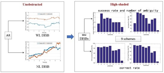
Although considerable research achievements in tight integration methods have been reported in the relative positioning field, studies on tight integration in UPD-based PPP-AR methods remain scarce. Khodabandeh and Teunissen [26] presented multi-system estimable parameters by applying the S-system theory, and intersystem biases were estimated using multi-system PPP-RTK full-rank models. We believe that tight integration theory is also suitable for point positioning ambiguity resolution using UPD. The tight integration method can provide more ambiguities to satisfy the requirement of the least number of fixed ambiguities for fixed-coordinate solutions, particularly in a high-shade environment. If the number of fixed ambiguities is less than the minimum number, a fixed-coordinate solution cannot be acquired. One of the major objectives of this study was to propose a tight integration kinematic UPD-based PPP-AR algorithm using overlapping frequencies. Similar to relative positioning, additional DISBs must be solved in PPP-AR to ensure that the between-system differenced ambiguities are integers. However, the estimation methods of the DISB are completely different. Considering that PPP utilizes undifferenced ionosphere-free combination observations rather than dual-differenced uncombined observations and the ambiguity combinations vary, using the same DISB estimation method as that for relative positioning is not appropriate. The proposed DISB estimation and utilization approach was explored in detail in this study. This may evolve into an option for future applications, based on the traditional PPP-AR method. The additional ambiguities provided by the tight integration method are valuable for users in highly obstructed environments. A kinematic PPP-AR experiment was conducted under a scenario with an extremely low number of observations to highlight the advantages of tight integration. We assumed that the receiver moves from an open field to a highly obstructed area where only a few satellites can be detected. The proposed tightly integrated PPP-AR method is expected to hold a continuous fixed state for as long as possible under difficult observational conditions. In our approach, the fixed-integer ambiguity information of the last epoch is used to solve the AR problem.

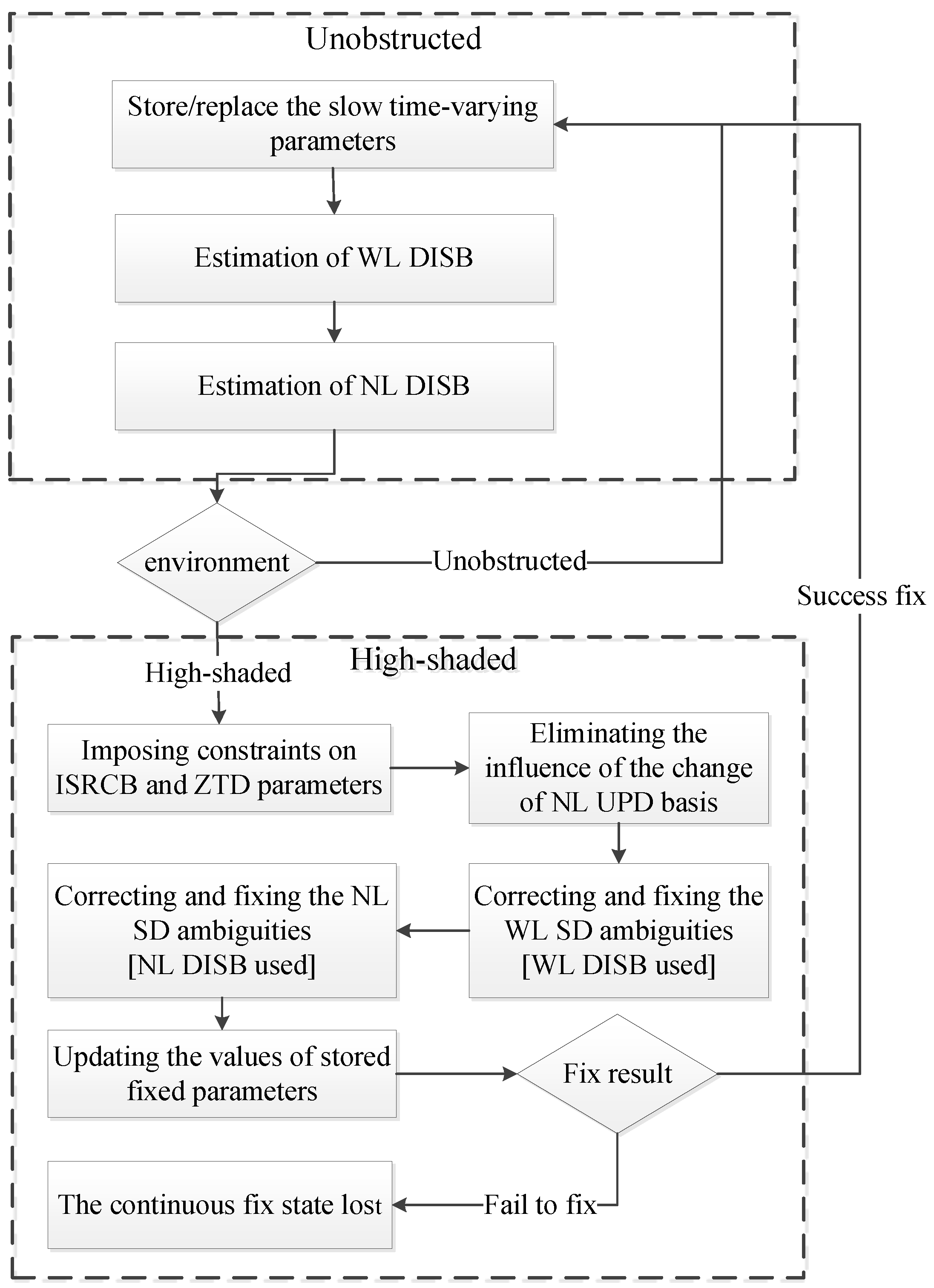
First, we briefly introduce the traditional PPP-AR model based on UPD products. Subsequently, we present the processing steps required as long as the receiver can gather a large number of observations, such as integer ambiguity information storage and wide lane (WL)/narrow lane (NL) DISB estimation. Next, we introduce the tight integration PPP-AR processing flow and key algorithms used when the receiver detects a drastic reduction in the number of observed satellites. This includes accounting for a change in the reference satellite and therefore the UPD reference, imposing constraints on zenith tropospheric delay (ZTD) parameters, usage of DISB, and the utilization of integer ambiguity information of the last epoch. Finally, kinematic PPP-AR experiments are conducted in a highly shaded observation environment to prove the effectiveness of the proposed method.

2. Methods

The ionosphere-free (IF) observations used in the traditional PPP model are expressed as

$$\left.\begin{array}{c}{P}_{\mathrm{I}\mathrm{F}}^s+{ct}_{\mathrm{I}\mathrm{F}}^s-{\rho }^s=c{t}_{\mathrm{I}\mathrm{F}}+c{t}_{\mathrm{G}\mathrm{x}}+T^s+{\epsilon }_{\mathrm{I}\mathrm{F},P}^s\\ {{\lambda }_{\mathrm{I}\mathrm{F}}\mathrm{\Phi }}_{\mathrm{I}\mathrm{F}}^s+c{t}_{\mathrm{I}\mathrm{F}}^s-{\rho }^s=c{t}_{\mathrm{I}\mathrm{F}}+c{t}_{\mathrm{G}\mathrm{x}}+T^s+{\mathrm{\lambda }}_{\mathrm{I}\mathrm{F}}{\tilde{N}}_{\mathrm{I}\mathrm{F}}^s+{\epsilon }_{\mathrm{I}\mathrm{F},\mathrm{\Phi }}^s\end{array}\right\}$$

(1)

where $P \mathrm{a}\mathrm{n}\mathrm{d} \mathrm{\Phi }$ denote code and phase observations, respectively, $\rho$ is the receiver-to-satellite geometric distance, and c is the speed of light. Superscript s denotes the satellite. $T^s$ denotes slant tropospheric delay, $t_{\mathrm{I}\mathrm{F}}$ and $t_{\mathrm{I}\mathrm{F}}^s$ are the receiver and satellite IF clock errors, respectively, and ${\tilde{N}}_{\mathrm{I}\mathrm{F}}^s$ represents float ambiguities in cycles with wavelength $\mathrm{\lambda }$. $\epsilon$ denotes observation noise. The difference in the receiver clocks between the GPS and other systems (written as x in [1]) $t_{\mathrm{G}\mathrm{x}}$ is estimated as a constant over 30 min. $t_{\mathrm{I}\mathrm{F}}$ is the updated epoch by epoch, and the wet tropospheric zenith delay (ZTD) residual is estimated hourly as a constant. The Saastamoinen mapping function was used in the present study. The AR process begins after the PPP calculation is completed.

2.1. Traditional Kinematic PPP-AR Model

First, the traditional PPP-AR model is briefly introduced. At the server, UPD products are generated and sent to users. Float WL ambiguities were calculated using the Melbourne–Wübbena (MW) combination. Furthermore, the float NL ambiguities are derived using float IF ambiguities estimated with (1) and fixed WL ambiguities. The float WL and NL ambiguity ${\tilde{N}}_r^s$ can be expressed as

$${\tilde{N}}_r^s=N_r^s+b_r+b^s+{\epsilon }_r^s$$

(2)

where the superscript ‘s’ refers to a satellite, whereas the subscript ‘r’ refers to a receiver. $N_r^s$ is the associated integer ambiguity of ${\tilde{N}}_r^s$. $b_r$ and $b^s$ are the receiver- and satellite-dependent UPDs, respectively. Once the ambiguities are solved for all j reference stations that commonly track k satellites, they can be computed as

$$\left[\begin{array}{c}{\tilde{N}}_1^1\\ {\tilde{N}}_1^2\\ \begin{array}{c}⋮\\ {\tilde{N}}_1^k\\ \begin{array}{c}{\tilde{N}}_2^1\\ ⋮\\ {\tilde{N}}_j^k\end{array}\end{array}\end{array}\right]=\left[\begin{array}{c}{N}_1^1\\ N_1^2\\ \begin{array}{c}⋮\\ N_1^k\\ \begin{array}{c}{N}_2^1\\ ⋮\\ N_j^k\end{array}\end{array}\end{array}\right]+\left[\begin{array}{cc}{\mathit{I}}_j\otimes {\mathit{e}}_k& {\mathit{e}}_j⨂{\mathit{I}}_k\end{array}\right]\left[\begin{array}{c}{b}_1\\ ⋮\\ \begin{array}{c}{b}_j\\ b^1\\ \begin{array}{c}⋮\\ b^k\end{array}\end{array}\end{array}\right]$$

(3)

where e_n denotes an n-dimensional column vector whose elements are all 1’s and I_n denotes an n-dimensional identity matrix. Regarding eliminating rank deficiency in (3), refer to Wang et al. [27] for further details. Next, the UPD is sent to the user together with the precise orbit and clock products.

Once the PPP calculation was completed at each epoch, the AR module was started. First, between-satellite single-differenced (SD) ambiguities were generated. Limited by the existing DISB, only two satellites from the same GNSS can be used to calculate a single SD ambiguity. The received UPDs were used to correct the WL SD ambiguities. After the NL SD ambiguities were estimated using IF and fixed WL ambiguities, they were revised using the corresponding UPDs. Assuming that the two satellites s and v are from the same system, the correction process is as follows:

$$\left.\begin{array}{c}{{\hat{N}}_{\mathrm{W}\mathrm{L},u}^{sv}=\tilde{N}}_{\mathrm{W}\mathrm{L},u}^{sv}+b_{\mathrm{W}\mathrm{L}}^s-b_{\mathrm{W}\mathrm{L}}^v\\ {{\hat{N}}_{\mathrm{N}\mathrm{L},u}^{sv}=\tilde{N}}_{\mathrm{N}\mathrm{L},u}^{sv}+b_{\mathrm{N}\mathrm{L}}^s-b_{\mathrm{N}\mathrm{L}}^v\end{array}\right\}$$

(4)

where $\tilde{N}$ is the UPD-biased float ambiguity, and $\hat{N}$ is the UPD-corrected float ambiguity. Subscript u denotes the receiver of the user. After correcting the SD ambiguities, WL ambiguities were rounded and NL ambiguities were fixed using the LAMBDA method. For the kinematic PPP-AR model, AR was performed at each epoch, and the fixed coordinates were stored if the ratio test was successful.

The proposed tightly integrated PPP-AR method using multi-GNSS overlapping frequency signals is an optional application module based on the traditional PPP-AR method. The new approach consists of DISB estimation in a good observation environment and DISB utilization in a high-shade situation. With the WL/NL DISB parameters and fixed ambiguity information acquired in an open environment, we assume that the hold time of the continuous fixed state can be longer, even though fewer than nine satellites can be observed. The two aspects are discussed in this section.

2.2. Estimation of WL/NL DISB Parameters in an Open Area

There are two types of receiver-related hardware biases: code range and phase range. The code range bias is introduced into the phase observation along with the receiver clock and intersystem receiver clock bias (ISRCB) parameters. Finally, together with the phase component, the introduced range hardware delay is absorbed by ambiguities. When the SD ambiguities are calculated using two-phase observations from the same system, receiver-related hardware delays can be eliminated. Here, it is necessary to introduce the difference between ISRCB and DISB. The ISRCB is the intersystem bias (ISB) of receiver clocks of different systems. The ISRCB reflects that the range-related receiver hardware delays of various GNSS systems are different. The ISRCB parameter introduces the range-related biases into the phase observations. As for the DISB in this work, it is estimated using the fractional part of the ambiguities, which contains both phase-related receiver hardware delays and the introduced range-related delays. It helps to decrease the intersystem hardware bias absorbed by the ambiguities, and retrieve the integer characteristic. However, two problems are associated with the ambiguities of different systems. One is the frequency. Ambiguity at different frequencies cannot be directly combined. Once overlapping frequency signals are used, this problem is solved. However, another problem is the varying hardware delays for different systems, which is still an imperative issue. We attempted to estimate the DISB to fix the differences in the hardware delays of the various systems. However, specific fixed parameters must be stored prior to processing.

2.2.1. Store/Replace the Slow Time-Varying Parameters

Because ISRCB and ZTD are stable over a short period [28], the ambiguities are subsequently fixed using the traditional PPP-AR method, and the fixed-ambiguity-constrained ISRCB and ZTD parameters are stored in ${\stackrel{-}{\mathit{x}}}_{\mathrm{l}\mathrm{a}\mathrm{s}\mathrm{t}}$. In contrast, integer ambiguities are stored or updated in ${\stackrel{-}{\mathit{N}}}_{\mathrm{l}\mathrm{a}\mathrm{s}\mathrm{t}}$. Although unnecessary information is generally erased in the software data processing of kinematic positioning after the real-time coordinate solution is calculated to save memory space, in our approach, ${\stackrel{-}{\mathit{x}}}_{\mathrm{l}\mathrm{a}\mathrm{s}\mathrm{t}}$ and ${\stackrel{-}{\mathit{N}}}_{\mathrm{l}\mathrm{a}\mathrm{s}\mathrm{t}}$ are retained.

2.2.2. Estimation of WL DISB

The undifferenced (UD) WL UPD-corrected ambiguity is expressed as follows:

$${{\hat{N}}_{\mathrm{W}\mathrm{L},\mathrm{A}}^s=\tilde{N}}_{\mathrm{W}\mathrm{L},\mathrm{A}}^s+b_{\mathrm{W}\mathrm{L}}^s$$

(5)

where ${\tilde{N}}_{\mathrm{W}\mathrm{L},r,\mathrm{A}}^s$ is the raw float WL ambiguity of satellite s from System A, and ${\hat{N}}_{\mathrm{W}\mathrm{L},\mathrm{A}}^s$ is its after-corrected value. The receiver-related WL hardware delay should be the fractional part of ${\hat{N}}_{\mathrm{W}\mathrm{L},\mathrm{A}}^s$, which is expressed as

$${h_{\mathrm{W}\mathrm{L},\mathrm{A}}^s=\tilde{N}}_{\mathrm{W}\mathrm{L},\mathrm{A}}^s-\left[{\hat{N}}_{\mathrm{W}\mathrm{L},\mathrm{A}}^s\right]$$

(6)

where $h_{\mathrm{W}\mathrm{L},\mathrm{A}}^s$ is the WL hardware delay of satellite s and [] is the symbol of rounding a number to the nearest integer. As WL ambiguities are influenced by observation noise, the fraction parts are not identical for the ambiguities of different satellites. The final hardware delay is the weighted average value, which is expressed as

$$h_{\mathrm{W}\mathrm{L},\mathrm{A}}=\frac{{\sum }_{s=1}^j\left(h_{\mathrm{W}\mathrm{L},\mathrm{A}}^s{p}^s\right)}{{\sum }_{s=1}^j\left(p^s\right)}$$

(7)

where $p^s$ denotes the weight determined by the elevation angle of satellite s, and $h_{\mathrm{W}\mathrm{L},\mathrm{A}}$ is the estimated WL hardware delay of System A. The WL DISB between systems A and B is expressed as

$${\delta }_{\mathrm{W}\mathrm{L},\mathrm{A}-\mathrm{B}}=h_{\mathrm{W}\mathrm{L},\mathrm{A}}-h_{\mathrm{W}\mathrm{L},\mathrm{B}}$$

(8)

In this study, the GPS was chosen as reference System B. The ${\delta }_{\mathrm{W}\mathrm{L},\mathrm{A}-\mathrm{B}}$ values of all the observed systems relative to the GPS were calculated and stored.

2.2.3. Estimation of NL DISB

Similar to the estimation method of WL DISB, UPD-corrected UD NL ambiguities were used to calculate NL DISB as follows:

$${{\hat{N}}_{\mathrm{N}\mathrm{L},\mathrm{A}}^s=\tilde{N}}_{\mathrm{N}\mathrm{L},\mathrm{A}}^s+b_{\mathrm{N}\mathrm{L}}^s$$

(9)

Because the wavelength is short and no between-satellite difference calculation is conducted, the accuracy and reliability of NL ambiguities are easily affected by various errors. Thus, the original UD NL ambiguities are too rough to estimate high-quality DISB. To ensure that the estimated DISB was sufficiently precise, we utilized SD-ambiguity-constrained UD NL ambiguities rather than original ambiguities. After the SD NL ambiguities are fixed, the constrained solution of all UD ambiguities and their corresponding cofactor matrix can be resolved as

$$\left.\begin{array}{c}{\stackrel{-}{\mathit{N}}}^{\mathrm{U}\mathrm{D}}={\hat{\mathit{N}}}^{\mathrm{U}\mathrm{D}}-{\mathit{Q}}_{{\hat{\mathit{N}}}^{\mathrm{U}\mathrm{D}}}{\mathit{S}}^T{\left(\mathit{S}{\mathit{Q}}_{{\hat{\mathit{N}}}^{\mathrm{U}\mathrm{D}}}{\mathit{S}}^T\right)}^{-1}\left({\hat{\mathit{N}}}^{\mathrm{S}\mathrm{D}}-{\mathit{N}}^{\mathrm{S}\mathrm{D}}\right)\\ {\mathit{Q}}_{{\stackrel{-}{\mathit{N}}}^{\mathrm{U}\mathrm{D}}}={\mathit{Q}}_{{\hat{\mathit{N}}}^{\mathrm{U}\mathrm{D}}}-{\mathit{Q}}_{{\hat{\mathit{N}}}^{\mathrm{U}\mathrm{D}}}{\mathit{S}}^T{\left(\mathit{S}{\mathit{Q}}_{{\hat{\mathit{N}}}^{\mathrm{U}\mathrm{D}}}{\mathit{S}}^T\right)}^{-1}\mathit{S}{\mathit{Q}}_{{\hat{\mathit{N}}}^{\mathrm{U}\mathrm{D}}}\end{array}\right\}$$

(10)

where ${\stackrel{-}{\mathit{N}}}^{\mathrm{U}\mathrm{D}}$ and ${\hat{\mathit{N}}}^{\mathrm{U}\mathrm{D}}$ are the constrained and UPD-corrected UD ambiguity (from Equation (9)) sets and their corresponding cofactor matrices are ${\mathit{Q}}_{{\stackrel{-}{\mathit{N}}}^{\mathrm{U}\mathrm{D}}}$ and ${\mathit{Q}}_{{\hat{\mathit{N}}}^{\mathrm{U}\mathrm{D}}}$, respectively. $\mathit{S}$ is the transformation matrix from the UD to SD ambiguities. ${\hat{\mathit{N}}}^{\mathrm{S}\mathrm{D}}$ and ${\mathit{N}}^{\mathrm{S}\mathrm{D}}$ are the UPD-corrected float and integer SD ambiguities, respectively. The precision of the UD ambiguities was improved by applying the constraints of the fixed SD ambiguities. Moreover, after constraining the fractional parts of the constrained UD, the NL ambiguities are very close to each other because the differences in the UD ambiguities are constrained to integers. The receiver-related NL hardware delay of System A should be the fraction of any UD ambiguity from System A, which is expressed as

$$h_{\mathrm{N}\mathrm{L},\mathrm{A}}={\stackrel{-}{N}}_{\mathrm{N}\mathrm{L},\mathrm{A}}^s-\left[{\stackrel{-}{N}}_{\mathrm{N}\mathrm{L},\mathrm{A}}^s\right]$$

(11)

where ${\stackrel{-}{N}}_{\mathrm{N}\mathrm{L},\mathrm{A}}^s$ is any constrained UD ambiguity from System A, and $h_{\mathrm{N}\mathrm{L},\mathrm{A}}$ is the receiver-related NL hardware delay of System A. The NL DISB between systems A and B is expressed as

$${\delta }_{\mathrm{N}\mathrm{L},\mathrm{A}-\mathrm{B}}=h_{\mathrm{N}\mathrm{L},\mathrm{A}}-h_{\mathrm{N}\mathrm{L},\mathrm{B}}$$

(12)

Similarly, the GPS was chosen as reference System B. The ${\delta }_{\mathrm{N}\mathrm{L},\mathrm{A}-\mathrm{B}}$ values of all observed systems relative to the GPS were calculated and stored. If g GNSSs are observed, the number of WL and NL DISBs are both equal to g−1.

As long as a sufficient number of observable satellites are available, the abovementioned processing steps are conducted every epoch. Until the number of observable satellites diminishes to no more than 3g, i.e., in a shaded/obstructed environment, the tight integration AR method is invoked. Taking g = 3 as an example, the estimated parameters, except ambiguities, are three coordinate elements, one ZTD, one receiver clock, and two ISRCBs, making seven in total. This implies that at least seven fixed SD ambiguities are required, which is not a difficulty in open areas. However, in a poor observation environment, although nine satellites are observed, because each system must be assigned a reference satellite, the total observed SD ambiguities are only six for the traditional AR approach, which means that a fixed-coordinate solution is impossible. However, the tight integration AR method, which can provide two additional ambiguities, is believed to enable the user to successfully obtain the final fixed solution. In the next subsection, the use of DISB in high-occlusion situations is introduced.

2.3. Tight Integration AR Method in a Highly Obstructed Situation

In contrast to the traditional PPP-AR method, some necessary constraints and revisions must be applied before calculating SD ambiguities.

2.3.1. Imposing Constraints on ISRCB and ZTD Parameters

In a short time period, both ISRCB and ZTD parameters can be treated as constants. Therefore, the ambiguity-constrained parameters acquired from the last epoch can be used as known values to impose constraints on the corresponding parameters of the current epoch. There are three reasons for restricting these two parameters. First, the constraint can directly decrease the number of estimated parameters, which must be fixed. The parameters imposed on the strong constraints no longer require the revision of fixed ambiguities. Second, the accuracy of all parameters is improved with the constraint. The third reason is the uniformity of the ISRCB and DISB. The range hardware delay is contained in both the ISRCB and ambiguities. In contrast, the stored ISRCB is the ambiguity-constrained solution at the last epoch, and the DISBs are estimated from fixed ambiguities. Thus, ISRCB and DISB from the last epoch were in fairly good agreement. To ensure optimal DISB performance, the ISRCB must be constrained to the stored value. When a user enters a highly obstructed environment, the fixed ISRCB and ZTD parameters stored in ${\stackrel{-}{\mathit{x}}}_{\mathrm{l}\mathrm{a}\mathrm{s}\mathrm{t}}$ are utilized, as follows:

$$\left.\begin{array}{c}\stackrel{-}{\mathit{y}}=\tilde{\mathit{y}}-{\mathit{Q}}_{\tilde{\mathit{y}}\tilde{\mathit{x}}}{\mathit{Q}}_{\tilde{\mathit{x}}}^{-1}\left(\tilde{\mathit{x}}-{\stackrel{-}{\mathit{x}}}_{\mathrm{l}\mathrm{a}\mathrm{s}\mathrm{t}}\right)\\ {\mathit{Q}}_{\stackrel{-}{\mathit{y}}}={\mathit{Q}}_{\tilde{\mathit{y}}}-{\mathit{Q}}_{\tilde{\mathit{y}}\tilde{\mathit{x}}}{\mathit{Q}}_{\tilde{\mathit{x}}}^{-1}{\mathit{Q}}_{\tilde{\mathit{x}}\tilde{\mathit{y}}}\end{array}\right\}$$

(13)

where $\tilde{\mathit{x}}$ covers the estimated ISRCB and ZTD of the current epoch, the cofactor matrices of which are ${\mathit{Q}}_{\tilde{\mathit{x}}}$. $\tilde{\mathit{y}}$ and $\stackrel{-}{\mathit{y}}$ are the before-constrained and after-constrained estimated parameters, respectively, except for ISRCB and ZTD. ${\mathit{Q}}_{\tilde{\mathit{y}}}$ and ${\mathit{Q}}_{\stackrel{-}{\mathit{y}}}$ are the corresponding cofactor matrices. ${\mathit{Q}}_{\tilde{\mathit{x}}\tilde{\mathit{y}}}$ is the cross-cofactor matrix between $\tilde{\mathit{x}}$ and $\tilde{\mathit{y}}$.

2.3.2. Eliminating the Influence of the Change in NL UPD Reference

Generally, a satellite with the highest elevation is used as a reference for UPD processing. In addition, the UPD reference of each GNSS is independent and individually defined. As a result, the basis can be eliminated in loose integration. However, in tight integration, the validity of DISBs is directly influenced by the jump in the basis. The DISB estimated at the last epoch cannot match the UPDs at the current epoch if the reference satellite for the UPD changes. Thus, the UPD gap between the two epochs must be detected and revised to ensure consistency between UPD and DISB.

The mean of NL UPDs is believed not to change significantly if the reference satellite is not transformed. The mean of the UPD of j satellites from System A at the ith epoch is expressed as:

$$b_{\mathrm{A},\mathrm{c}}(i)=\frac{{\sum }_{s=1}^j\left(b_{\mathrm{N}\mathrm{L}}^s\right)}{s}$$

(14)

where $b_{\mathrm{A},\mathrm{c}}\left(i\right)$ is the UPD barycenter. The difference in the UPD barycenter between epochs i and i−1 is

$${dif}_{\mathrm{A},c}=b_{\mathrm{A},\mathrm{c}}\left(i\right)-b_{\mathrm{A},\mathrm{c}}(i-1)$$

(15)

When the absolute value of ${dif}_{A,c}$ is greater than the empirical value of 0.05 cycle, the DISB needs to be revised.

$${\stackrel{-}{\delta }}_{\mathrm{N}\mathrm{L},\mathrm{A}-\mathrm{B}}={\delta }_{\mathrm{N}\mathrm{L},\mathrm{A}-\mathrm{B}}+{dif}_{\mathrm{A},c} \mathrm{or} {\stackrel{-}{\delta }}_{\mathrm{N}\mathrm{L},\mathrm{B}-\mathrm{A}}={\delta }_{\mathrm{N}\mathrm{L},\mathrm{B}-\mathrm{A}}-{dif}_{\mathrm{A},c}$$

(16)

where ${\stackrel{-}{\delta }}_{\mathrm{N}\mathrm{L},\mathrm{A}-\mathrm{B}}$ and ${\stackrel{-}{\delta }}_{\mathrm{N}\mathrm{L},\mathrm{B}-\mathrm{A}}$ are the after-revised DISBs.

2.3.3. Generating between-Satellite SD Ambiguities

In addition to the SD ambiguities of satellite pairs in every system, satellites with the highest elevation angle in each system were selected to calculate tight integration ambiguities. Among all the NL SD ambiguities, the integer ambiguities that have been fixed at the last epoch with no cycle slip discovered at the current epoch are termed as ${\mathit{N}}_{\mathrm{N}\mathrm{L},l}$ in this study.

2.3.4. Correcting and Fixing the WL SD Ambiguities

For tight integration ambiguities of satellites from different systems, UPD and DISB are utilized to correct the errors and restore the integer characteristics.

$${{\hat{N}}_{\mathrm{W}\mathrm{L}}^{sv}=\tilde{N}}_{\mathrm{W}\mathrm{L}}^{sv}+b_{\mathrm{W}\mathrm{L}}^s-b_{\mathrm{W}\mathrm{L}}^v-{\delta }_{\mathrm{W}\mathrm{L},\mathrm{A}-\mathrm{B}}$$

(17)

where s and v are two satellites from systems A and B, respectively, and ${\tilde{N}}_{\mathrm{W}\mathrm{L}}^{sv}$ and ${\hat{N}}_{\mathrm{W}\mathrm{L}}^{sv}$ are the before- and after-corrected tight integration WL ambiguities, respectively. The ${\hat{N}}_{\mathrm{W}\mathrm{L}}^{sv}$ are currently prepared to be fixed.

2.3.5. Correcting and Fixing the NL SD Ambiguities

The NL float ambiguities can be estimated using fixed WL ambiguities and float IF ambiguities ${\tilde{N}}_{\mathrm{I}\mathrm{F}}^s$ from (1). Similar to WL ambiguities, NL ambiguities are also revised using DISB and UPD as follows:

$${{\hat{N}}_{\mathrm{N}\mathrm{L}}^{sv}=\tilde{N}}_{\mathrm{N}\mathrm{L}}^{sv}+b_{\mathrm{N}\mathrm{L}}^s-b_{\mathrm{N}\mathrm{L}}^v-{\delta }_{\mathrm{N}\mathrm{L},\mathrm{A}-\mathrm{B}}$$

(18)

where ${\tilde{N}}_{\mathrm{N}\mathrm{L}}^{sv}$ and ${\hat{N}}_{\mathrm{N}\mathrm{L}}^{sv}$ are the before-corrected and corrected tight integration NL ambiguities, respectively.

It was assumed that no cycle slip was detected in the current epoch. In this case, the integer ambiguities at the last epoch, ${\mathit{N}}_{\mathrm{N}\mathrm{L},l}$, are reliable for restricting the corresponding ambiguities at the current epoch and improving their accuracy. Particularly in a high-shade environment, the constraint is critical for improving the quality of the new ambiguity appearing at the current epoch. The constraint is imposed as follows:

$$\left.\begin{array}{c}\stackrel{-}{\mathit{a}}=\tilde{\mathit{a}}-{\mathit{Q}}_{\tilde{\mathit{a}}{\hat{\mathit{N}}}_{\mathrm{N}\mathrm{L},l}}{\mathit{Q}}_{{\hat{\mathit{N}}}_{\mathrm{N}\mathrm{L},l}}^{-1}\left({\hat{\mathit{N}}}_{\mathrm{N}\mathrm{L},l}-{\mathit{N}}_{\mathrm{N}\mathrm{L},l}\right)\\ {\mathit{Q}}_{\stackrel{-}{\mathit{a}}}={\mathit{Q}}_{\tilde{\mathit{a}}}-{\mathit{Q}}_{\tilde{\mathit{a}}{\hat{\mathit{N}}}_{\mathrm{N}\mathrm{L},l}}{\mathit{Q}}_{{\hat{\mathit{N}}}_{\mathrm{N}\mathrm{L},l}}^{-1}{\mathit{Q}}_{{\hat{\mathit{N}}}_{\mathrm{N}\mathrm{L},l}\tilde{\mathit{a}}}\end{array}\right\}$$

(19)

where ${\hat{\mathit{N}}}_{\mathrm{N}\mathrm{L},l}$ is the UPD-corrected NL ambiguity vector at the current epoch calculated from (18), which has been fixed at the last epoch, and ${\mathit{Q}}_{{\hat{\mathit{N}}}_{\mathrm{N}\mathrm{L},l}}$ is the corresponding cofactor matrix; $\tilde{\mathit{a}}$ and $\stackrel{-}{\mathit{a}}$ are before-constraint and after-constraint estimated parameters, except ${\hat{\mathit{N}}}_{\mathrm{N}\mathrm{L},l}$, respectively; ${\mathit{Q}}_{\tilde{\mathit{a}}}$ and ${\mathit{Q}}_{\stackrel{-}{\mathit{a}}}$ are their corresponding cofactor matrices, respectively; ${\mathit{Q}}_{\tilde{\mathit{a}}{\hat{\mathit{N}}}_{\mathrm{N}\mathrm{L},l}}$ denotes the cofactor matrices of $\tilde{\mathit{a}}$ and ${\hat{\mathit{N}}}_{\mathrm{N}\mathrm{L},l}$. Finally, $\stackrel{-}{\mathit{a}}$ can be fixed using LAMBDA.

2.3.6. Updating the Values of Stored Fixed Parameters

After the ambiguities are successfully fixed, ${\mathit{N}}_{\mathrm{N}\mathrm{L},l}$ must be updated to the current value. As introduced in Section 2.2.3, assuming that three systems are observed, seven parameters are estimated in total. Thus, in this case, if the number of fixed SD ambiguities is not less than seven, both the ISRCBs and ZTD can be updated. However, the number of available satellites is severely limited in a high-shade environment (perhaps even fewer than nine satellites); together with the influence of partial AR, it is usually not sufficient to update all of the parameters, although the presented tight integration method has been utilized. Considering the various influences of different parameters on AR, the update priority of ISRCBs is higher than that of the ZTD. If the fixed ambiguity number is only six, the two ISRCBs are updated. The hold times of the two ISRCB parameters were compared when the number was as low as five. Assuming that the last update times of the two ISRCBs are $t_{A-B}$ and $t_{A-C}$, the ISRCB between systems A and C are updated when $t_{A-B}>t_{A-C}$, and between systems A and B when $t_{A-B}<t_{A-C}$. Furthermore, the DISBs are updated as in Section 2.2.2 and Section 2.2.3.

If the ambiguities cannot be fixed, the fixed state is lost, and the current output is the float coordinate solution. The entire procedure is shown in the flowchart in Figure 1.

3. Datasets and Evaluation Indicators

We used observational data from the IGS network with 40 reference stations in Asia, as shown in Figure 2, to generate UPDs. The UPDs of Galileo, GPS, and QZSS were calculated at 60 s intervals. The PTGG station from the Philippines was selected as the user, and its 1 s interval observations from 0:00 to 6:30 UTC (i.e., 8:00 to 14:30 local time) on 2 February 2022, were acquired to conduct the kinematic PPP-AR experiment. Although static experimental data from the reference station were utilized to simulate a user receiver, the kinematic PPP algorithm module was executed to demonstrate the performance of kinematic positioning. The user receiver type was a Septentrio PolaRx5 connected to a TRM59800.00 antenna. To realize tight integration of the PPP-AR method, GPS/Galileo/QZSS overlapping frequency signals were used, which were L1/L5 of GPS and QZSS, and E1/E5a of Galileo. In the PPP-AR experiment, the kinematic PPP engine was restarted every half-hour from 0:00 to 5:30, which means that the PPP was restarted 12 times. For each computation, one-hour data were utilized. No shelter was set in the first half-hour to ensure that the DISBs were precisely generated. The high-shade environment was artificially structured in the second half-hour to evaluate the PPP-AR performance using the proposed method. Several schemes of obstructed environments are elaborated on in the following section. The ambiguities were fixed at each epoch in the second half-hour. Only the AR performance in the second half-hour was counted. The ratio test was conducted once the ambiguities were fixed and the threshold was experientially set to 1.8.

Several evaluation indicators were selected to assess the AR results. The ratio between the duration of holding a continuous fixed state and the observation time is called the success fix rate, ${\mathrm{P}}_{\mathrm{s}\mathrm{f}}$. We checked the position errors derived with fixed ambiguities to further evaluate AR reliability. If the position error was less than the distance threshold of known coordinates, the fixed solution was assumed to be correct. The thresholds were 5/10/15 cm (H5/H10/H15) for the horizontal error and 10/15 cm (V10/V15) for the vertical error. The ratio between the number of correct fixed solutions was termed the correct fix rate, ${\mathrm{P}}_{\mathrm{c}\mathrm{f}}$. In addition, the number of fixed ambiguities was counted.

4. Results and Discussion

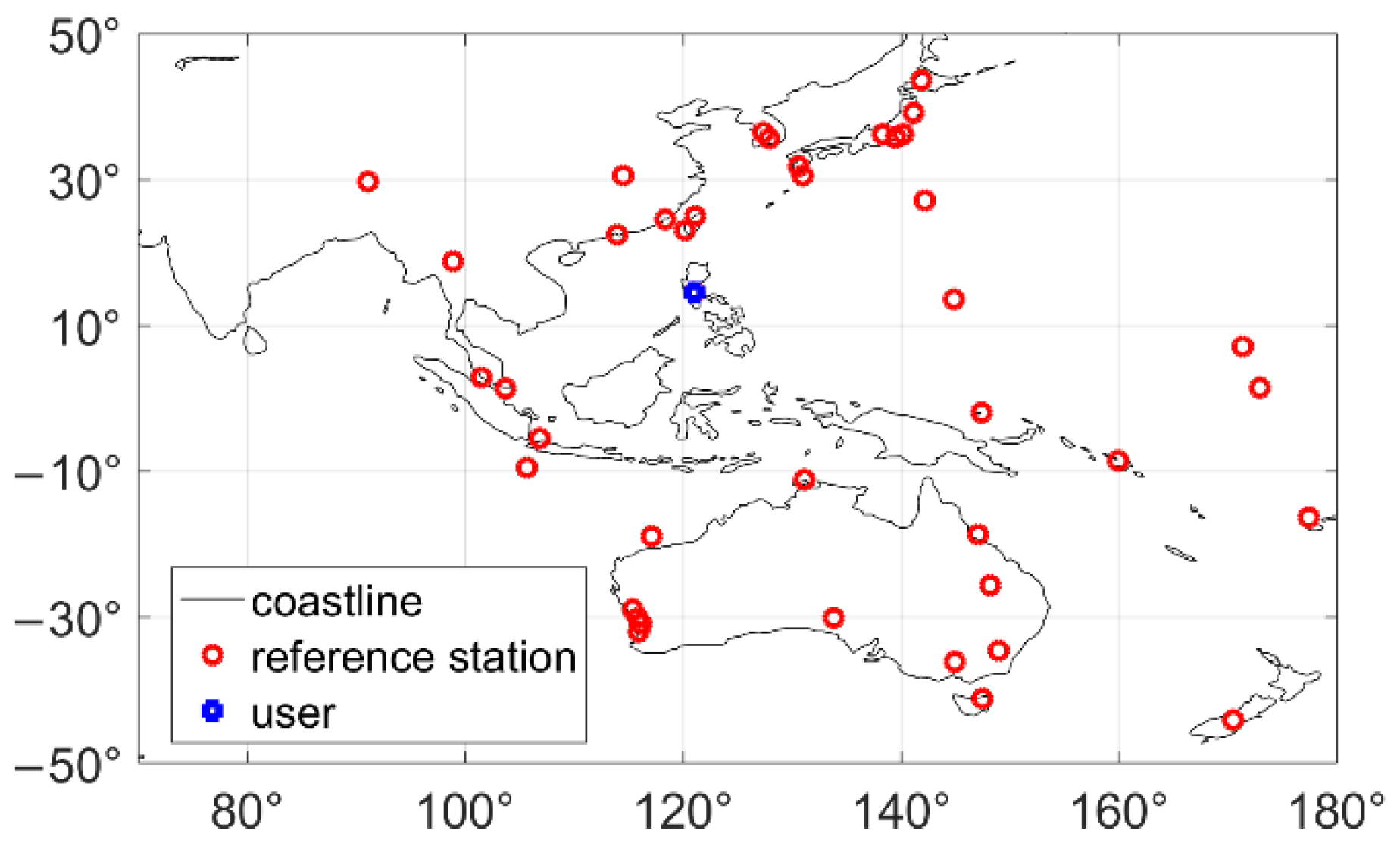
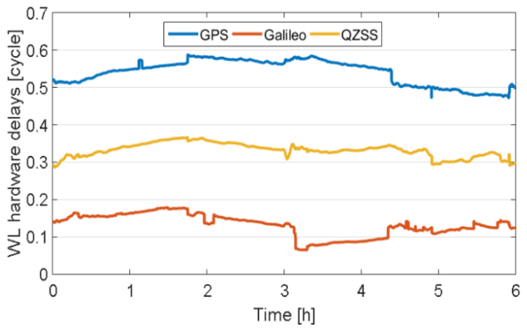
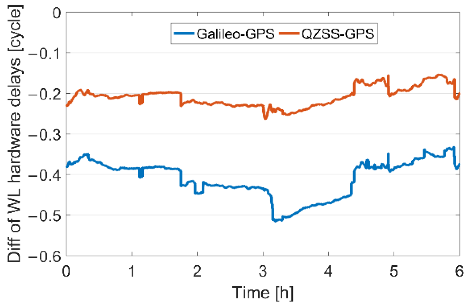
This section shows the WL and NL DISBs of the PTGG station estimated using the method presented in Section 2.2.2 and Section 2.2.3. The WL and NL receiver-related hardware delays for each GNSS from 0:00 to 6:00 are shown in Figure 3 and Figure 5, respectively. The WL and NL DISBs are displayed in Figure 4 and Figure 6, respectively.

The WL receiver-related hardware delays changed quite slowly with a maximal fluctuation range of approximately 0.15 cycles within 6 h. Occasional sudden jumps were generally caused by a cycle-slip occurrence, a newly observed satellite, or the disappearance of a satellite because of its low elevation angle. For the DISBs, the fluctuation range did not exceed 0.2 cycles. Because the GPS was selected as the reference system, Galileo-GPS and QZSS-GPS DISBs displayed similar fluctuations and trends.

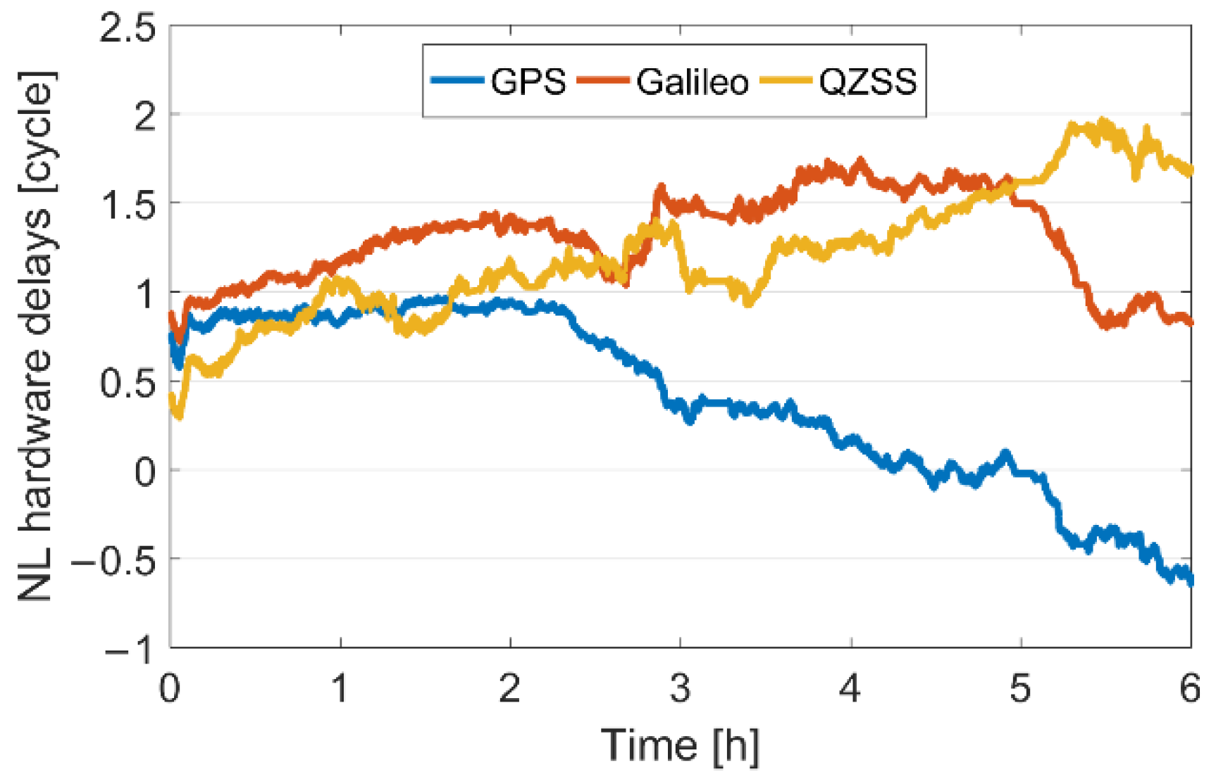
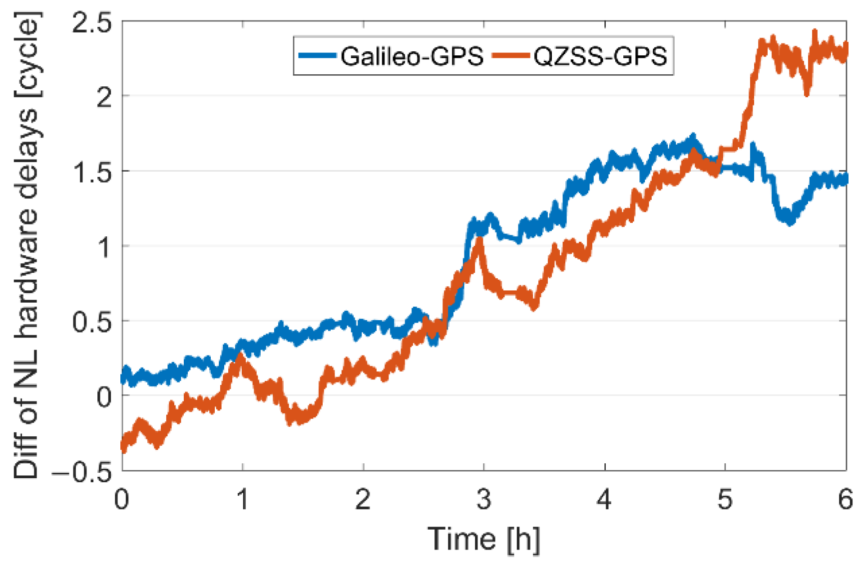
A change in the NL UPD reference basis can cause a sudden jump in NL receiver-related hardware delays; therefore, the influence of a discontinuous UPD reference basis was eliminated in Figure 5 and Figure 6. The fluctuation range of the NL hardware delays was larger than that of WL, reaching up to 1.6, 1.1, and 1.7 cycles for the GPS, Galileo, and QZSS, respectively. The GPS curve unexpectedly crossed 0.5 cycles in half an hour. As a result, the maximal ranges of DISBs were 1.7 and 2.8 cycles for Galileo-GPS and QZSS-GPS, respectively. Thus, NL DISBs must be updated frequently to maintain their reliability. However, the variation over a very short period was minimal. This implied that using the DISBs estimated in the last epoch in the proposed method was reasonable. Compared with the DISB results calculated using relative positioning observation equations [21], our DISBs showed slightly poor stability. This may be because a greater number of satellite-related or environment-related unmodeled errors were contained in ambiguities and final DISBs because between-receiver differenced observations cannot be acquired in the PPP-AR model.

The advantage of the tight integration AR method is highlighted in a high-shade environment because every extra ambiguity is essential for satellite geometry and ensuring an adequate number of fixed SD ambiguities. Kinematic PPP-AR experiments were conducted in a highly obstructed environment to demonstrate and evaluate the performance of the proposed method. Nine experimental schemes were designed to simulate various observational environments using different AR strategies and satellite data from different systems, as listed in

Table 1. Experimental schemes designed to simulate various observational environments.

Scheme	Integration Method	Number of Observed Satellites
		GPS	Galileo	QZSS
1	loose	3	3	3
2	tight	3	3	3
3	tight	2	3	3
4	tight	3	2	3
5	tight	3	3	2
6	tight	2	2	3
7	tight	2	3	2
8	tight	3	2	2
9	tight	2	2	2

.

The scheme “3 GPS, 3 Galileo, and 3 QZSS” refers to the top three satellites with the highest elevation angles of each system which can be observed in the second half-hour of each computation. We aimed to compare the AR results of the traditional loose integration approach and the proposed tight integration method. However, in Scheme 1, even if all six SD ambiguities are fixed, a fixed solution cannot be obtained because there are seven estimated parameters. Thus, the ZTD parameter was directly fixed to the precise value obtained during the first half-hour. When the number of observed satellites is further reduced, as shown in Schemes 3–9, the traditional loose integration becomes unavailable.

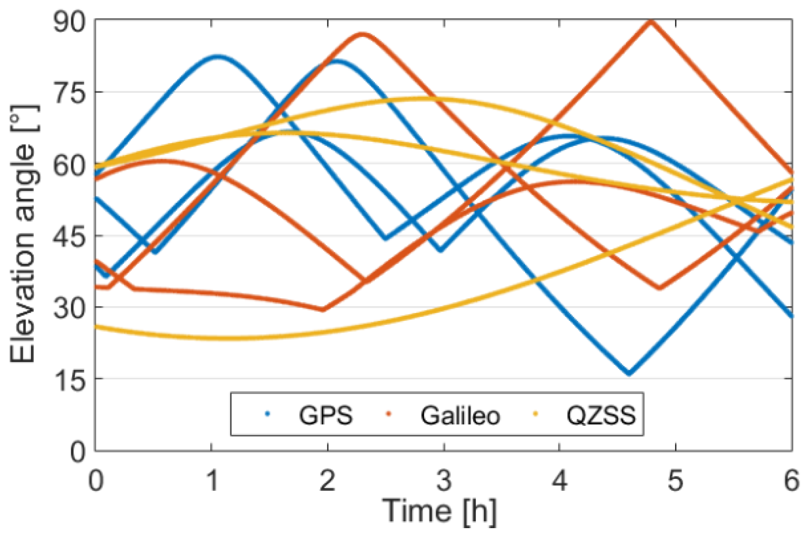
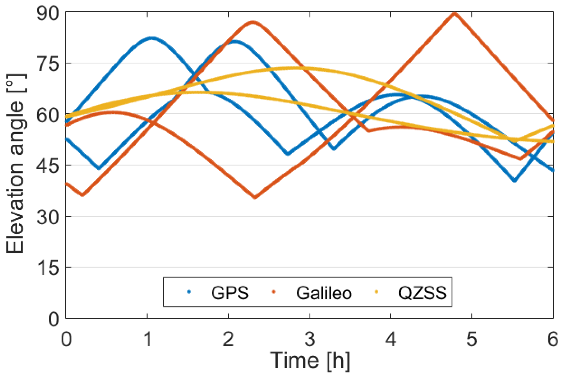
To intuitively display the satellite geometry when only three satellites can be observed for each system, Figure 7 and Figure 8 show the elevation angles of three and two satellites observed for each system, respectively. In Figure 7, the average elevation angle is approximately 50°, and the elevation angles of only two satellites are less than 30° over a fraction of time. In Figure 8, all elevation angles are greater than 35°, and almost all satellites are concentrated in the zenith direction. Only six satellites can be observed, and the satellite geometry is poor; therefore, AR is generally difficult in this situation.

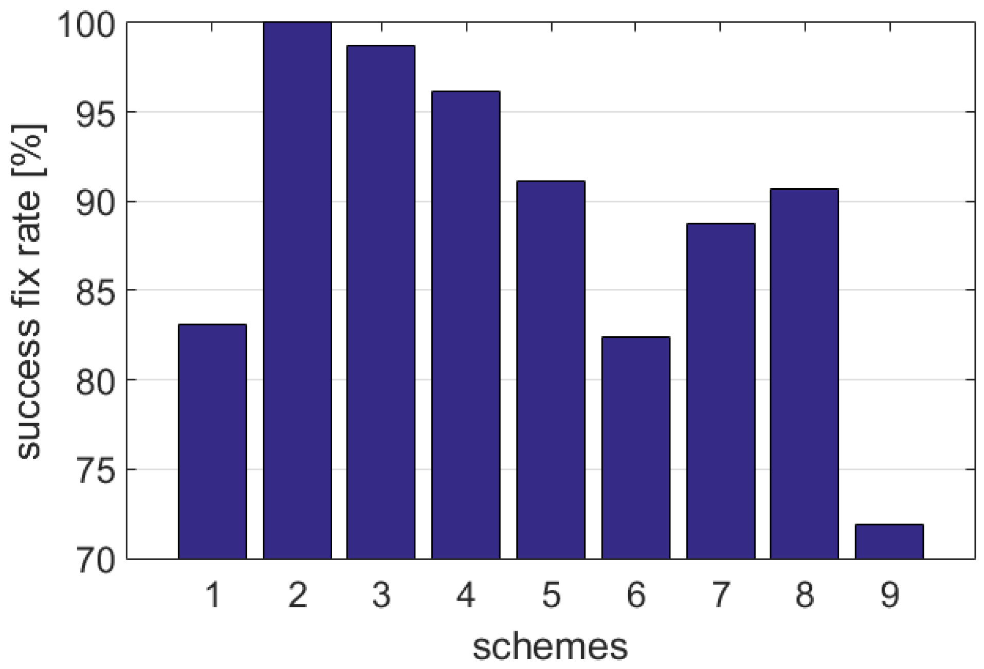
PPP-AR numerical experiments were conducted based on the design of the experiment introduced in Datasets and evaluation indicators, and the following statistical results were obtained. In the proposed method, fixed ambiguities from the last epoch are used to limit the current float ambiguities. This strategy ensures a continuous fixed state for a period after the user receiver enters a shaded environment. However, it is difficult to determine whether ambiguities can still be fixed when a cycle slip occurs, or when a new satellite is tracked, which largely determines the success fix rate. Figure 9 shows the average ${\mathrm{P}}_{\mathrm{s}\mathrm{f}}$ for all schemes. It should be noted that Schemes 1 and 2 should not be compared directly because the ZTD parameter of Scheme 1 was fixed before AR, whereas it remained floating in Scheme 2. Nevertheless, the ${\mathrm{P}}_{\mathrm{s}\mathrm{f}}$ improved from 83% to 100% after the tight integration method was used. Eight satellites were observed in Schemes 3–5, with ${\mathrm{P}}_{\mathrm{s}\mathrm{f}}$ values greater than 91%. For Schemes 6–8 with seven satellites, the ${\mathrm{P}}_{\mathrm{s}\mathrm{f}}$ range was 82–90%. However, when the number of satellites decreased to six, the ${\mathrm{P}}_{\mathrm{s}\mathrm{f}}$ was only 72%, even with tight integration.

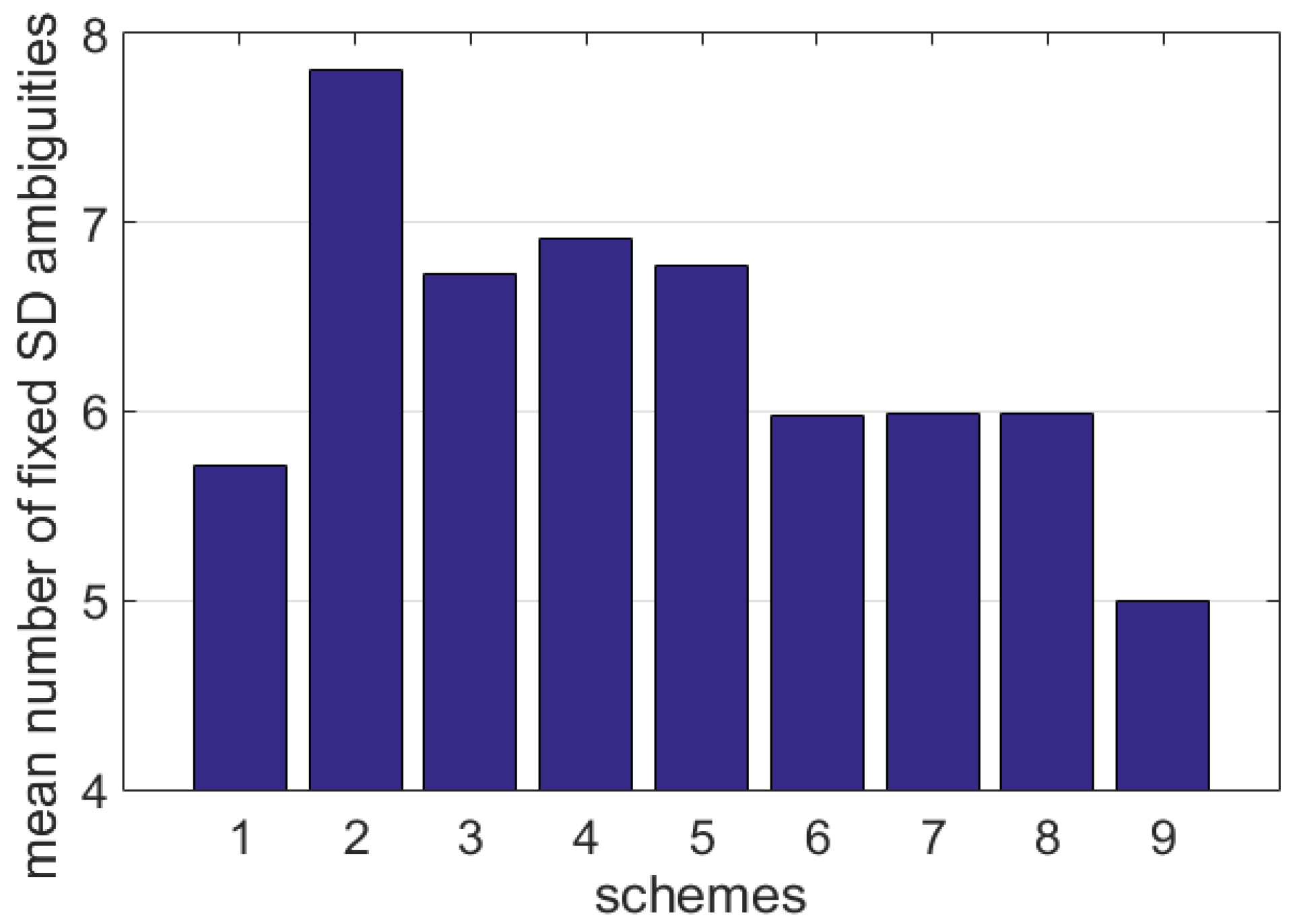
Figure 10 shows the average number of fixed SD ambiguities for all schemes. Compared to Scheme 1, Scheme 2 estimates two more intersystem SD ambiguities; therefore, the average fixed ambiguity number is increased by two. For Schemes 2–5, the resolution of a new NL ambiguity is delayed when it is not sufficiently precise or the WL ambiguity fails to be fixed. Thus, the continuous fix state will not be lost in this situation, owing to the relatively higher number of ambiguities. The number of available ambiguities is strictly limited for Schemes 6–9; therefore, once a new ambiguity replaces an old one and the new ambiguity is not precise enough to be fixed, the AR can hardly succeed because of the terrible satellite geometry. Thus, the average number of fixed ambiguities in Schemes 6–9 is close to an integer.

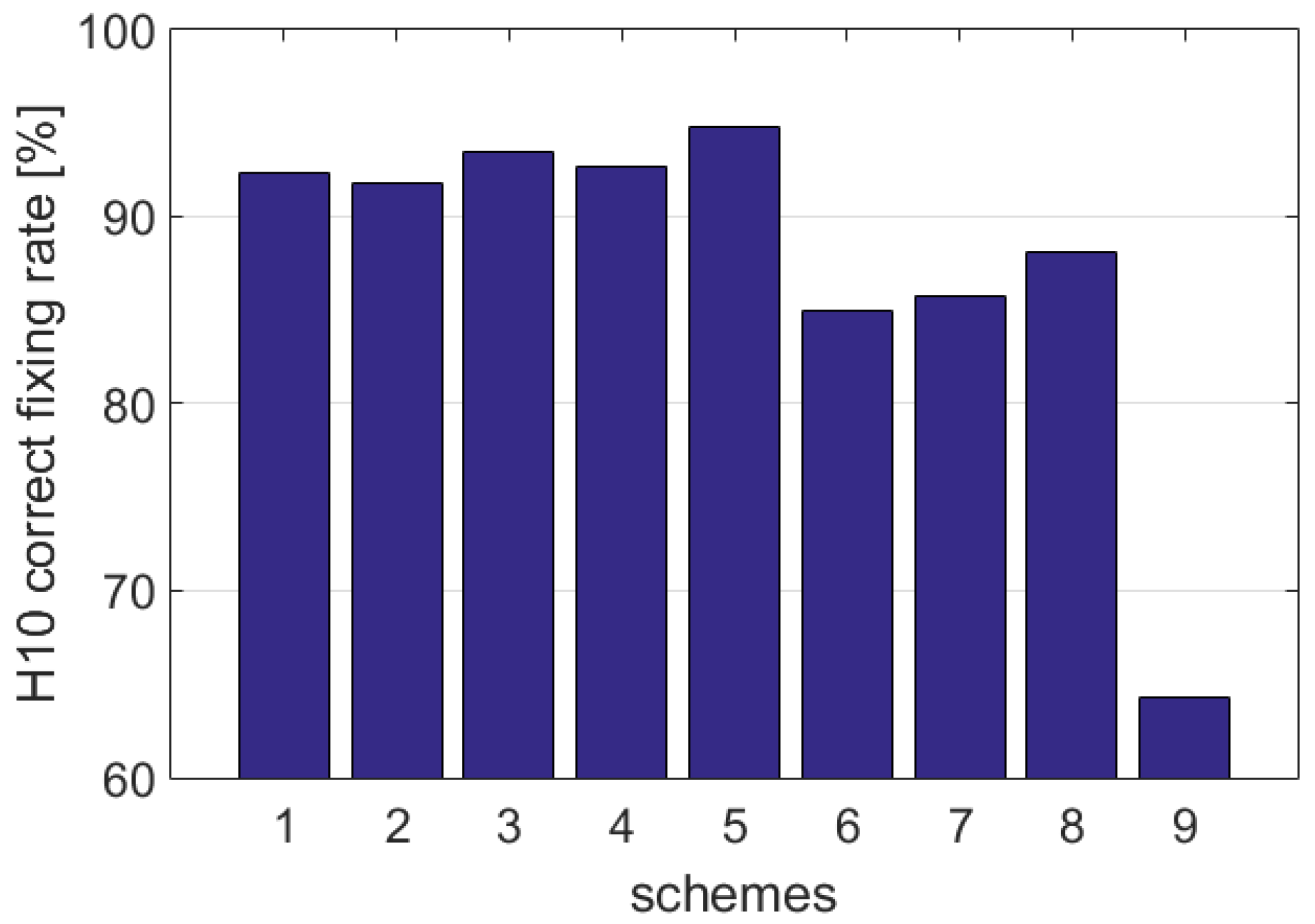
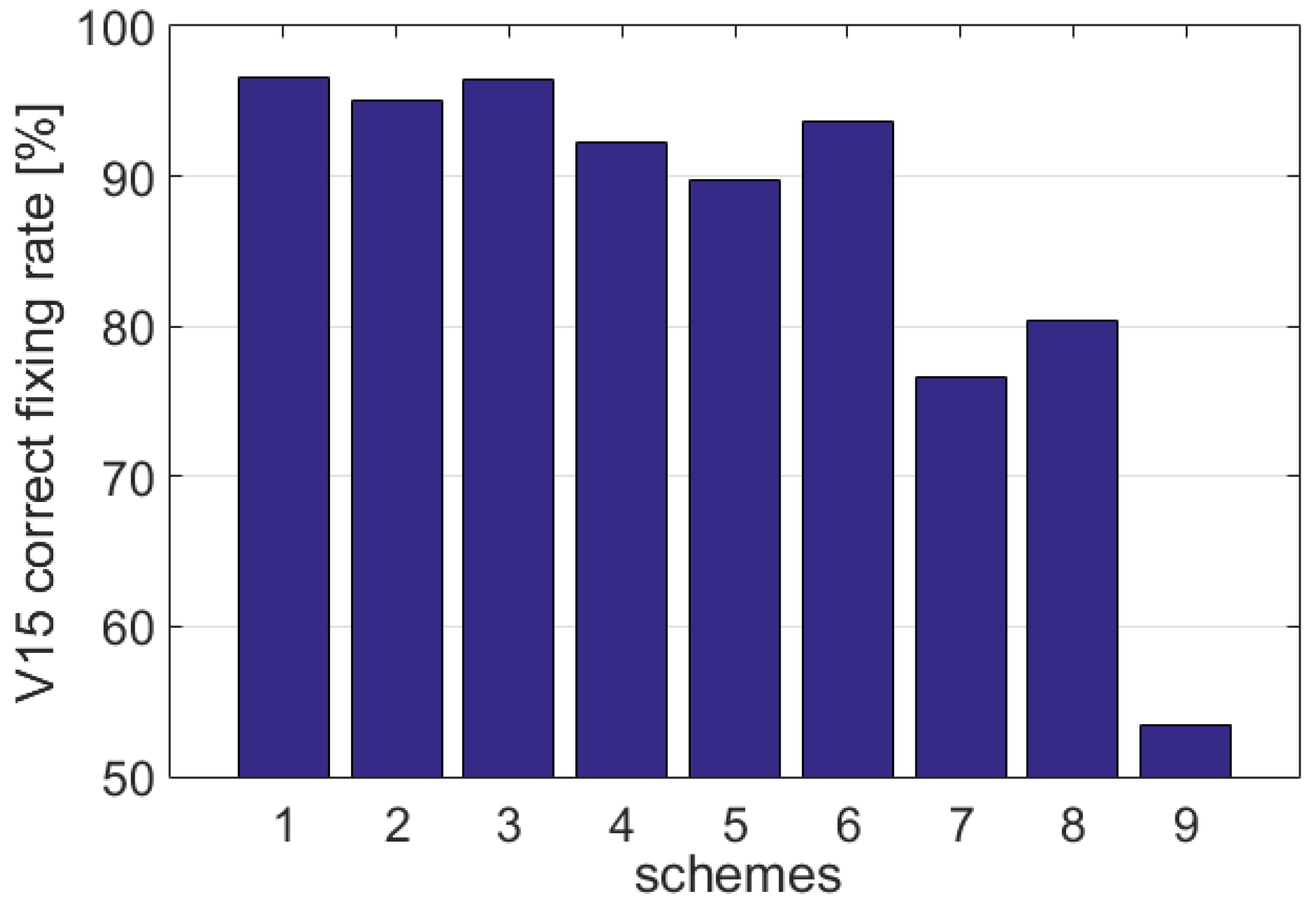
Figure 11 and Figure 12 show the average H10 and V15 ${\mathrm{P}}_{\mathrm{c}\mathrm{f}}$ values of all schemes, respectively. The detailed statistical results of ${\mathrm{P}}_{\mathrm{c}\mathrm{f}}$ for all position error thresholds are listed in

Table 2. Correct fixing rate according to the given error thresholds.

Scheme	1	2	3	4	5	6	7	8	9
H5 ${\mathrm{P}}_{\mathrm{c}\mathrm{f}}$ [%]	83.4	64.3	66.3	63.8	72.6	46.2	54.3	65.3	36.3
H10 ${\mathrm{P}}_{\mathrm{c}\mathrm{f}}$ [%]	92.4	91.7	93.4	92.7	94.8	84.9	85.7	88.0	64.3
H15 ${\mathrm{P}}_{\mathrm{c}\mathrm{f}}$ [%]	95.2	97.7	98.0	98.4	99.3	95.6	90.8	96.2	75.2
V10 ${\mathrm{P}}_{\mathrm{c}\mathrm{f}}$ [%]	84.7	82.8	86.8	83.1	79.5	74.9	65.1	66.4	46.2
V15 ${\mathrm{P}}_{\mathrm{c}\mathrm{f}}$ [%]	96.5	95.0	96.3	92.1	89.7	93.6	76.5	80.4	53.4

. The statistical results after further classification according to the satellite number are shown in

Table 3. Success fixing rate and correct fixing rate after classification according to the number of available satellites.

Number of Satellites	9	8	7	6
${\mathrm{P}}_{\mathrm{s}\mathrm{f}}$ [%]	100	95.3	87.2	71.9
H5 ${\mathrm{P}}_{\mathrm{c}\mathrm{f}}$ [%]	64.3	67.6	55.2	36.3
H10 ${\mathrm{P}}_{\mathrm{c}\mathrm{f}}$ [%]	91.7	93.6	86.2	64.3
H15 ${\mathrm{P}}_{\mathrm{c}\mathrm{f}}$ [%]	97.7	98.5	94.2	75.2
V10 ${\mathrm{P}}_{\mathrm{c}\mathrm{f}}$ [%]	82.8	83.1	68.8	46.2
V15 ${\mathrm{P}}_{\mathrm{c}\mathrm{f}}$ [%]	95.0	92.7	83.5	53.4
Number of fixed SD ambiguities	7.81	6.80	5.99	5.00

.

The lower the number of observed satellites, the lower the ${\mathrm{P}}_{\mathrm{c}\mathrm{f}}$. The H10 and V15 ${\mathrm{P}}_{\mathrm{c}\mathrm{f}}$ values are above 90% when eight or nine satellites were observed. However, the average H10 ${\mathrm{P}}_{\mathrm{c}\mathrm{f}}$ was only 86% and 64% and the average V15 ${\mathrm{P}}_{\mathrm{c}\mathrm{f}}$ values were 84% and 53% when the number of satellites was 7 and 6, respectively. For schemes in which the number of satellites are identical, the values of ${\mathrm{P}}_{\mathrm{c}\mathrm{f}}$ are quite similar, except for Scheme 6 in Figure 12. This is because the elevation angle of the QZSS satellite with the third highest elevation is relatively low; thus, its improvement in the vertical coordinate is more significant.

In conclusion, the proposed tightly integrated PPP-AR approach used overlapping frequency signals to improve the availability of fixed solutions markedly. The proposed method can still provide users with fixed-coordinate solutions for a period, particularly when the traditional kinematic PPP-AR method fails because of the lack of observed satellites.

5. Conclusions

This study presented a tightly integrated UPD-based PPP-AR approach using overlapping frequency signals to exploit the overlapping frequency signals of multi-GNSSs to improve the PPP-AR method. The detailed algorithm flow is introduced, including multiple parts such as integer ambiguity information storage, wide lane (WL)/narrow lane (NL) DISB estimation, accounting for a change in the UPD reference, imposing constraints on ZTD parameters, usage of DISB, and the utilization of integer ambiguity information of the last epoch. Finally, a series of kinematic PPP-AR experiments were conducted in a highly obstructed observation environment to demonstrate the effectiveness of the proposed method.

The WL receiver-related hardware delays were observed to change moderately, with a maximum fluctuation range of approximately 0.15 cycles within 6 h. However, the fluctuation range of NL hardware delays was larger than that of WL, reaching 1.6, 1.1, and 1.7 cycles for GPS, Galileo, and QZSS, respectively. The PPP-AR experiment results indicate that the ${\mathrm{P}}_{\mathrm{s}\mathrm{f}}$ improves from 83% to 100% after using the tight integration method compared with the traditional method in high-shade situations where only three satellites are tracked for each system. However, for the worst condition, in which fewer than nine satellites are tracked, the traditional method is futile, whereas the proposed method still produces fixed-coordinate solutions in our experiments.