Optimal Automatic Wide-Area Discrimination of Fish Shoals from Seafloor Geology with Multi-Spectral Ocean Acoustic Waveguide Remote Sensing in the Gulf of Maine

Abstract

Ocean Acoustic Waveguide Remote Sensing (OAWRS) enables fish population density distributions to be instantaneously quantified and continuously monitored over wide areas. Returns from seafloor geology can also be received as background or clutter by OAWRS when insufficient fish populations are present in any region. Given the large spatial regions that fish inhabit and roam over, it is important to develop automatic methods for determining whether fish are present at any pixel in an OAWRS image so that their population distributions, migrations and behaviour can be efficiently analyzed and monitored in large data sets. Here, a statistically optimal automated approach for distinguishing fish from seafloor geology in OAWRS imagery is demonstrated with Neyman–Pearson hypothesis testing which provides the highest true-positive classification rate for a given false-positive rate. Multispectral OAWRS images of large herring shoals during spawning migration to Georges Bank are analyzed. Automated Neyman-Pearson hypothesis testing is shown to accurately distinguish fish from seafloor geology through their differing spectral responses at any space and time pixel in OAWRS imagery. These spectral differences are most dramatic in the vicinity of swimbladder resonances of the fish probed by OAWRS. When such significantly different spectral dependencies exist between fish and geologic scattering, the approach presented provides an instantaneous, reliable and statistically optimal means of automatically distinguishing fish from seafloor geology at any spatial pixel in wide-area OAWRS images. Employing Kullback–Leibler divergence or the relative entropy in bits from Information Theory is shown to also enable automatic discrimination of fish from seafloor by their distinct statistical scattering properties across sensing frequency, but without the statistical optimal properties of the Neyman–Pearson approach.

1. Introduction

Fish populations comprise a large part of the marine biomass, play a major role in the inter-trophic chain and provide roughly $16\%$ of human protein consumption [1]. Concerns about adverse affects from climate change and overfishing have highlighted the need for ecosystem-scale sensing and monitoring of marine habitats [2]. Fish populations in ocean environments, however, are primarily monitored with highly localized line transect methods using high-frequency downward directed echo-sounders or capture trawl from slow-moving research vessels that significantly undersample populations in time and space, leaving an incomplete and ambiguous record of abundance and behavior [3,4,5].

Ocean Acoustic Waveguide Remote Sensing (OAWRS) has the potential to significantly improve sampling of oceanic fish populations and behavior to help sustain and properly manage the world’s fish populations. The OAWRS technology has been shown to enable instantaneous population density quantification and continuous monitoring of fish populations over thousands of square kilometers, with space-time sampling rates tens of thousands to millions of times higher than line transect methods by employing the natural capacity of the oceans for long-range sound channeling at lower frequencies [3,4,6]. Fish populations and behavior have been studied with OAWRS over wide areas in the Mid-Atlantic Bite [3], the Gulf of Maine [7] and the Nordic Seas [8,9,10,11]. To summarize some key results, the instantaneous horizontal structures and volatile short-term behavior of very large fish shoals, containing tens to hundreds of millions of fish and stretching for many kilometers, have been revealed by OAWRS, including the presence of population density waves within the shoals that exceed fish swimming speeds [3,7]. Theoretical predictions that a transition from random to synchronous group behavior should occur when a critical population density is attained have been proven in the natural environment with OAWRS imagery showing the formation and migration of massive spawning shoals of herring stretching for many kilometers over Georges Bank [7]. There, the depth of large upslope migrating fish shoals from deep waters to shallow spawning grounds was also remotely determined by multi-spectral OAWRS imagery, providing three-dimensional images of the shoals’ morphology [12]. Interactions between multi-species whale predators and spawning herring prey was revealed over tens of thousands of square kilometers in the Gulf of Maine using OAWRS [13]. Accurate enumeration of the entire Georges Bank herring spawning population was made from a single instantaneous OAWRS image per day over the 8-day peak spawning period, to within 7% of the independent NOAA estimate for 2006, which required weeks of surveying [8,14]. Cod spawning shoals sizes quantified with OAWRS in Lofoten Norway, with spatial diameters of up to roughly 40 km, were used to help quantify conditions leading to Cod stock collapses [8]. These results have been obtained in tandem with advances in accurately predicting and modeling the acoustic scattering from marine life that makes OAWRS possible [6,7,10,11,12,15,16,17,18,19,20] as well as with advances in equipment development for long-range, wide-area ocean acoustics sensing [21,22,23].

Since OAWRS instantaneously provides continuous spatial coverage over thousands of square kilometers, the seafloor is sometimes imaged when insufficient fish populations are present, assuming scattered returns are not ambient noise limited which is typically the case by design [3]. Currently, distinction between regions of fish versus seafloor geology in OAWRS imagery is achieved manually by [3,7] (1) analysis of the space-time dynamical patterns of prominent returns, (2) confirmation with highly localized measurements with trawls or downward directed echo sounders, which are limited to a very small subset of the areas instantaneously surveyed with OAWRS, and (3) analysis of differences in the frequency response between fish and seafloor, where such spectral methods have also enabled fish depth to be estimated [12,15,16,17].

Given the large open ocean habits of fish, and the large data sets produced by OAWRS, it is more efficient to have automated rather than manual procedures for distinguishing regions containing fish from those dominated by seafloor scattering [16] in OAWRS imagery. It is then a natural goal to employ an easily automated and statistically optimal methodology for making such a binary decision at any pixel in an OAWRS image. Such a methodology exists in Neyman–Pearson Hypothesis testing which delivers the maximum possible true positive decision rate for a given allowable false-positive rate [24], and so is the optimal approach for such automated decision making. We apply this approach to data collected during the OAWRS 2006 experiment in the Gulf of Maine [7] where multi-spectral OAWRS imagery is available at frequencies in the vicinity of the swimbladder resonances of the spawning herring shoals studied [12,15,16,17]. In this experiment, herring shoals were observed by OAWRS to form each day in deep waters at the northern flank of Georges bank near sunset and to migrate to shallow waters on Georges Bank to spawn. The analysis here is conducted using examples of multi-spectral OAWRS images of these spawning shoals at various days during the spawning period, which was observed to last for roughly one week. Since the herring frequency response is significantly different [12,17] from the frequency response of seafloor scattering [16], this data set is particularly well suited to automatically distinguishing fish from seafloor at each pixel in an OAWRS image. The automatic classification is performed by choosing between two competing hypotheses, one corresponding to fish shoals dominating the scattered returns with their characteristic frequency response and the other for seafloor scattering with its characteristic frequency response, using theoretically and empirically determined multivariate probability density functions for scattering strength from the herring shoals and those for the seafloor [12,15,16,17,25,26,27].

The statistically optimal and automated approach presented here should significantly help to identify, analyze and monitor fish population densities over the very large oceanic regions they inhabit.

2. Materials and Methods

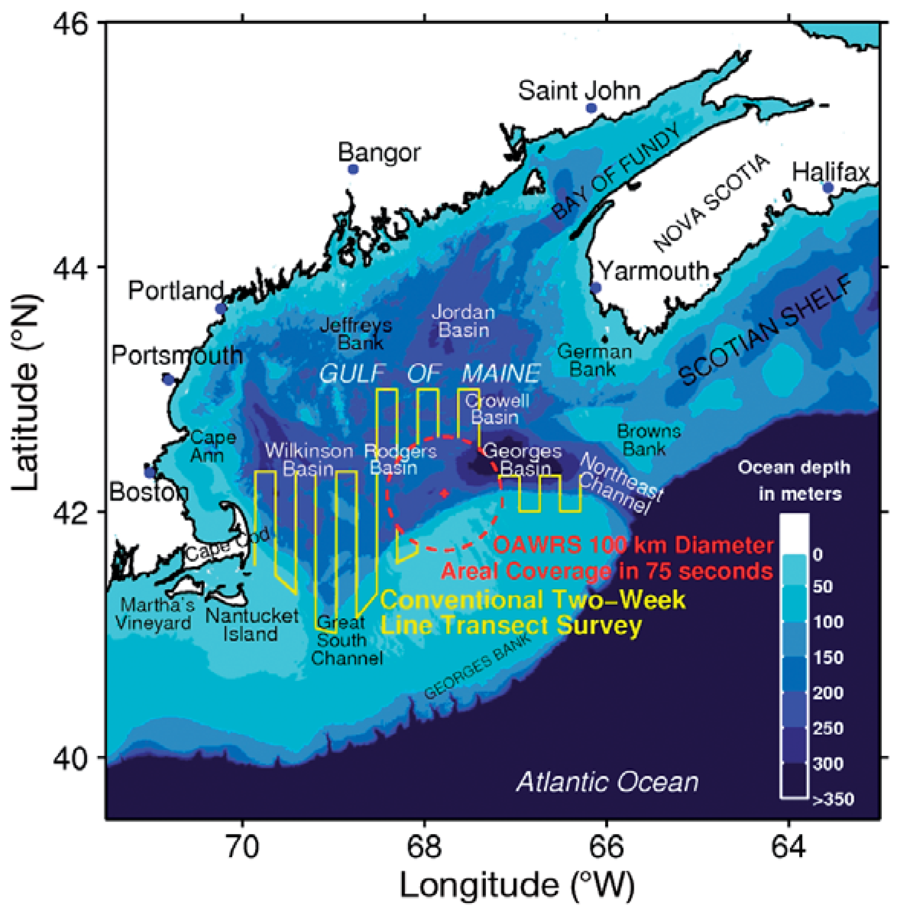
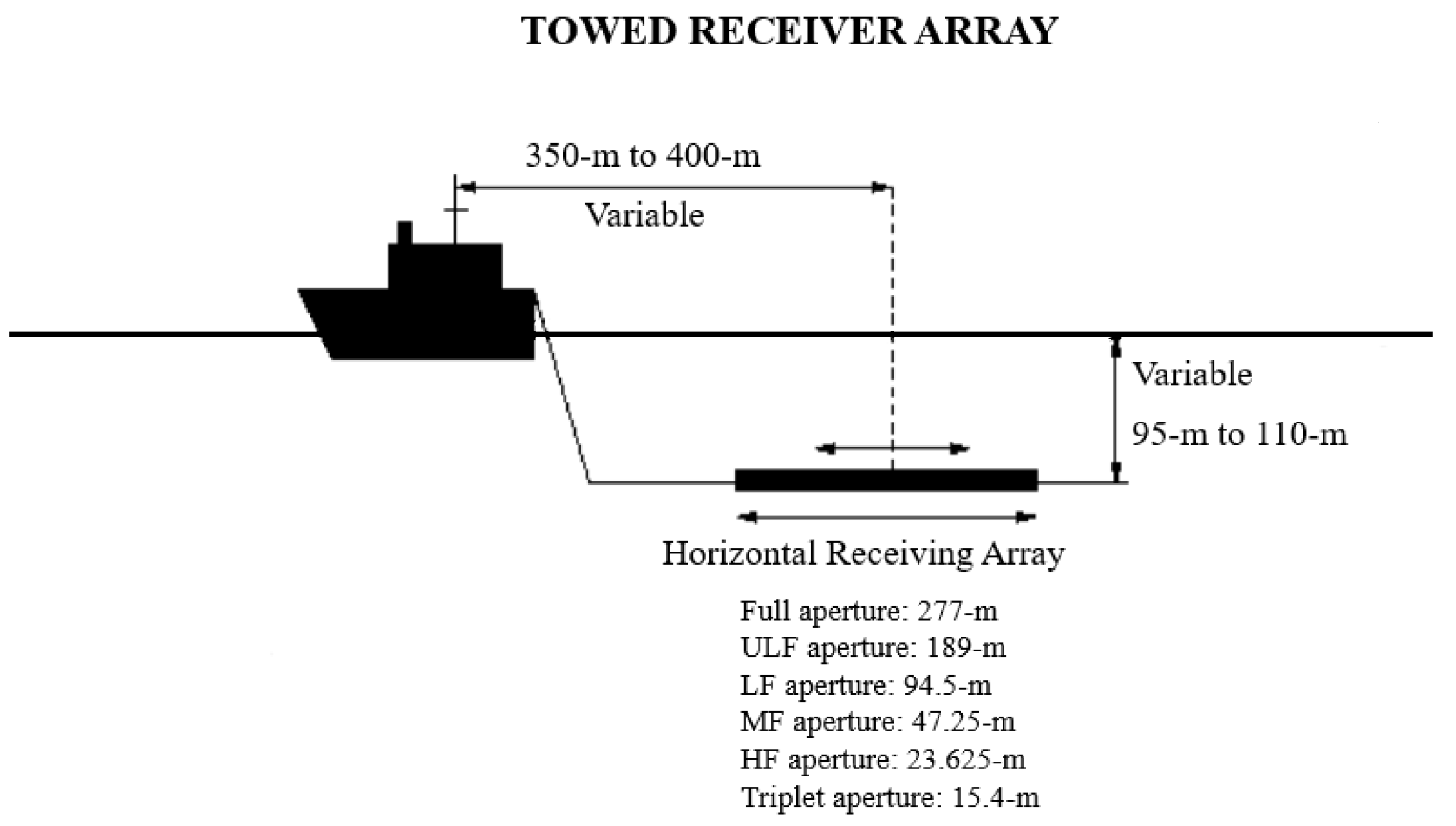
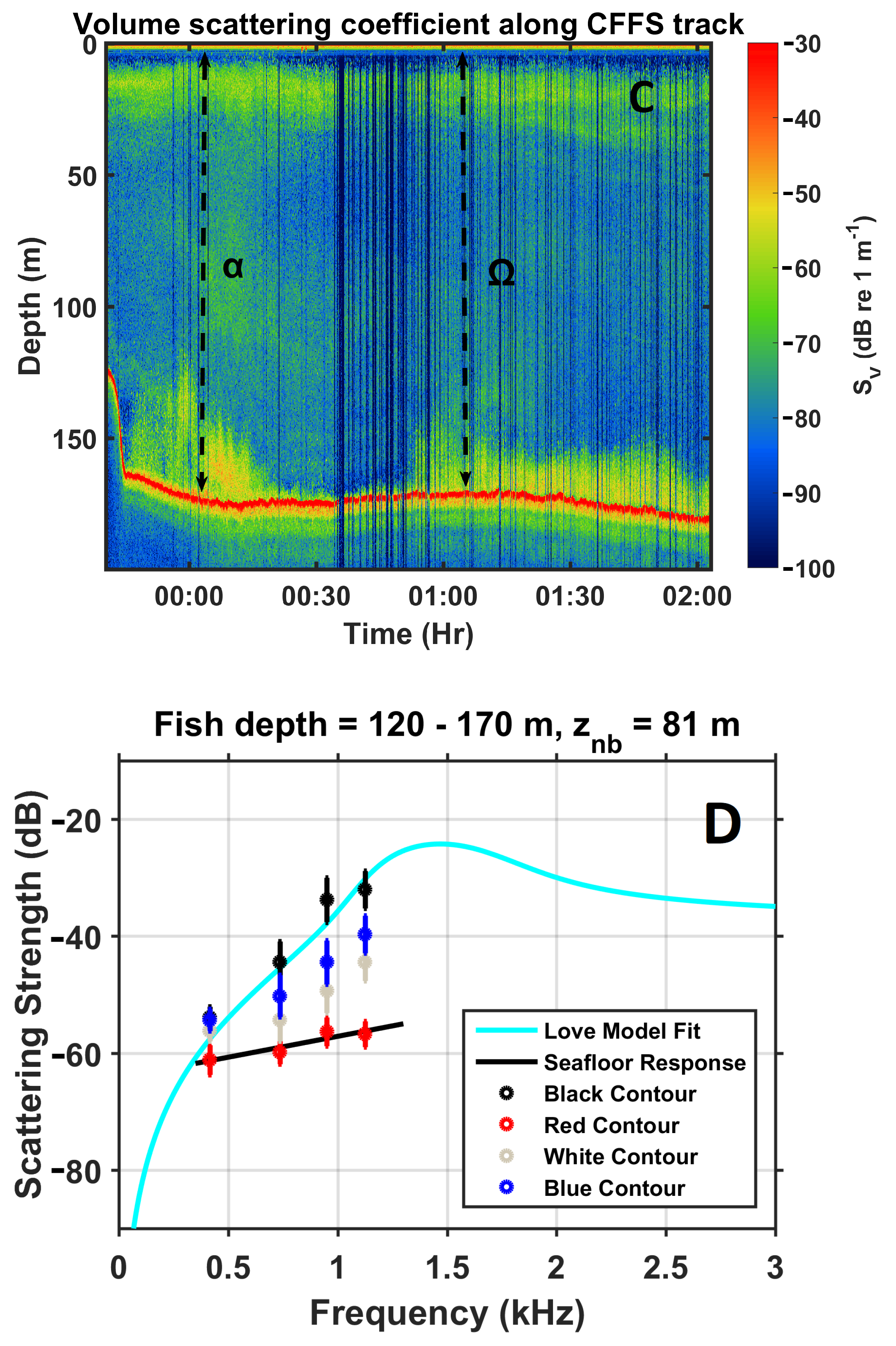
2.1. OAWRS Gulf of Maine 2006 Experiment

The data presented here are from the Gulf of Maine 2006 OAWRS Experiment (Figure 1) conducted on the western flank of Georges Bank area from 19 September to 6 October 2006, in conjunction with the U.S. National Marine Fisheries Service Annual Atlantic Herring Acoustic Survey [4,5,14]. In this experiment, spatial and temporal population density distributions, group behavior and physical scattering characteristics of Atlantic Herring (Clupea harengus) were quantified during their annual spawning period in their primary spawning ground in the Gulf of Maine [6,7,8,10,12,13,16,17,18,19,28].

Fish aggregations were instantaneously imaged over a 100 km diameter area and continuously monitored with consecutive image updates in a complex continental-shelf environment with variable bathymetry and oceanography [7]. The herring shoals imaged by OAWRS typically corresponded to tens to hundreds of millions of individuals, and extended for many kilometers across the western flank of Georges Bank. Simultaneously, ground truth sampling of herring shoals identified by OAWRS was performed with local downward directed echo-sounding and concurrent trawl sampling from supporting research vessels.

In this experiment, the OAWRS system employed a vertical source array to transmit linear frequency modulated (LFM) pulses centered at a range of frequencies from 390 to 1150 Hz and with 50 Hz bandwidth and 1 s duration [7,12,17]. Scattered returns from the environment were received with a horizontal towed line array with multiple nested sub-apertures at half-wavelength sensor spacing spanning 5 octaves (Figure 2). Three 64-element apertures were used in this analysis, with inter-element spacing of 1.5 m, 0.75 m and 0.375 m nominally for the low (LF), mid (MF) and high frequency (HF), respectively [29]. Beamforming coherently combining all sensors in these three apertures is employed here to obtain the high resolution in horizontal azimuth [30]. This eventually leads to a fixed range resolution of roughly 15 m, and an azimuthal resolution varying as $\lambda /(Lcos\theta )$ in radians away from array endfire, where $\theta$ is the scan angle from array broadside, $\lambda$ is the acoustic wavelength and L is the array aperture length. Matched filtering with the transmitted waveform follows beamforming, which is in turn followed by spatial charting of scattered returns [3,7,17,31,32]. Instantaneous snapshots of the ocean environment over the two-way travel times of the scattered returns are then obtained with sufficient imaging resolution to investigate the group behavior of oceanic fish over vast regions.

2.2. Automatic Distinction of Fish Shoals from Seafloor in Multi-Spectral OAWRS Imagery via Neyman–Pearson Hypothesis Testing

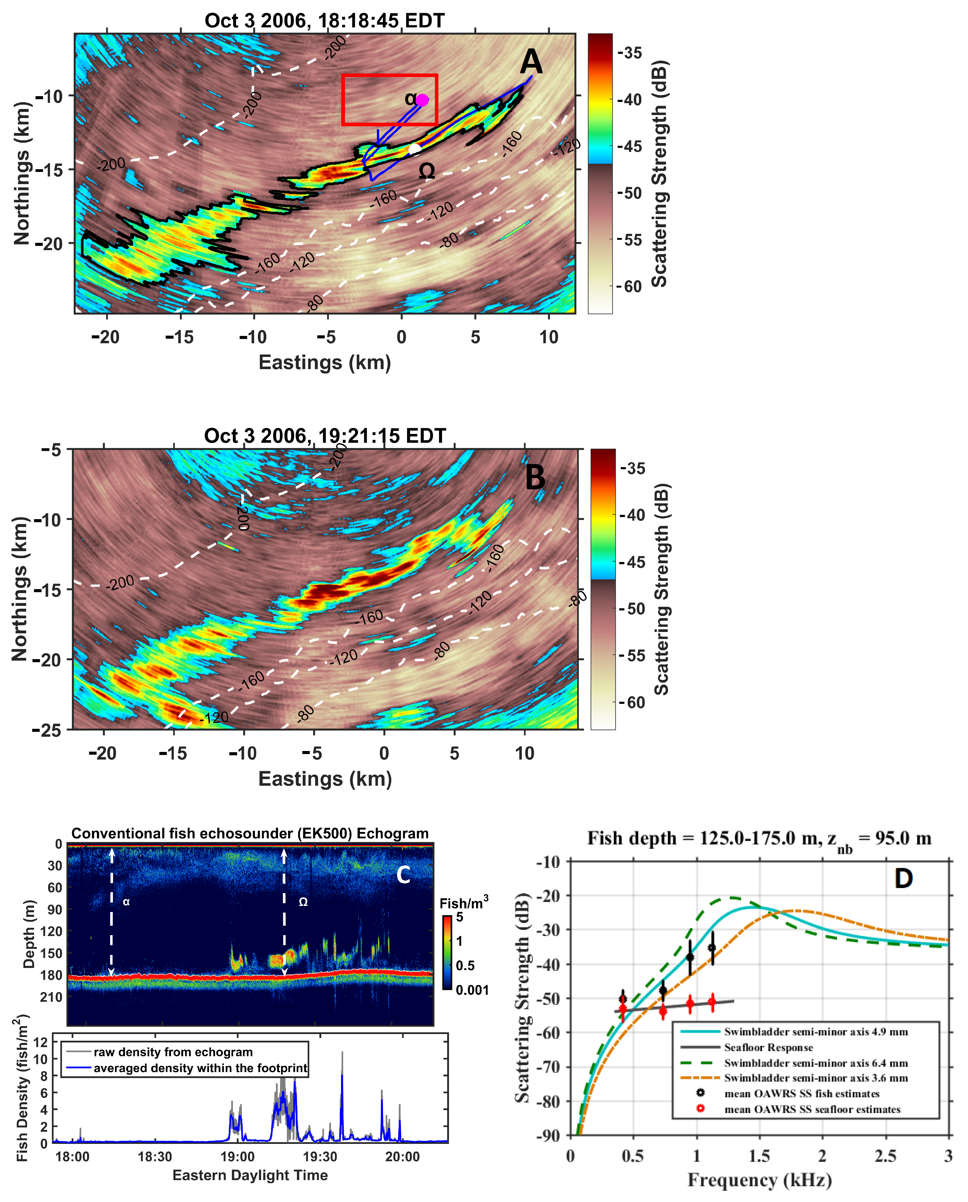
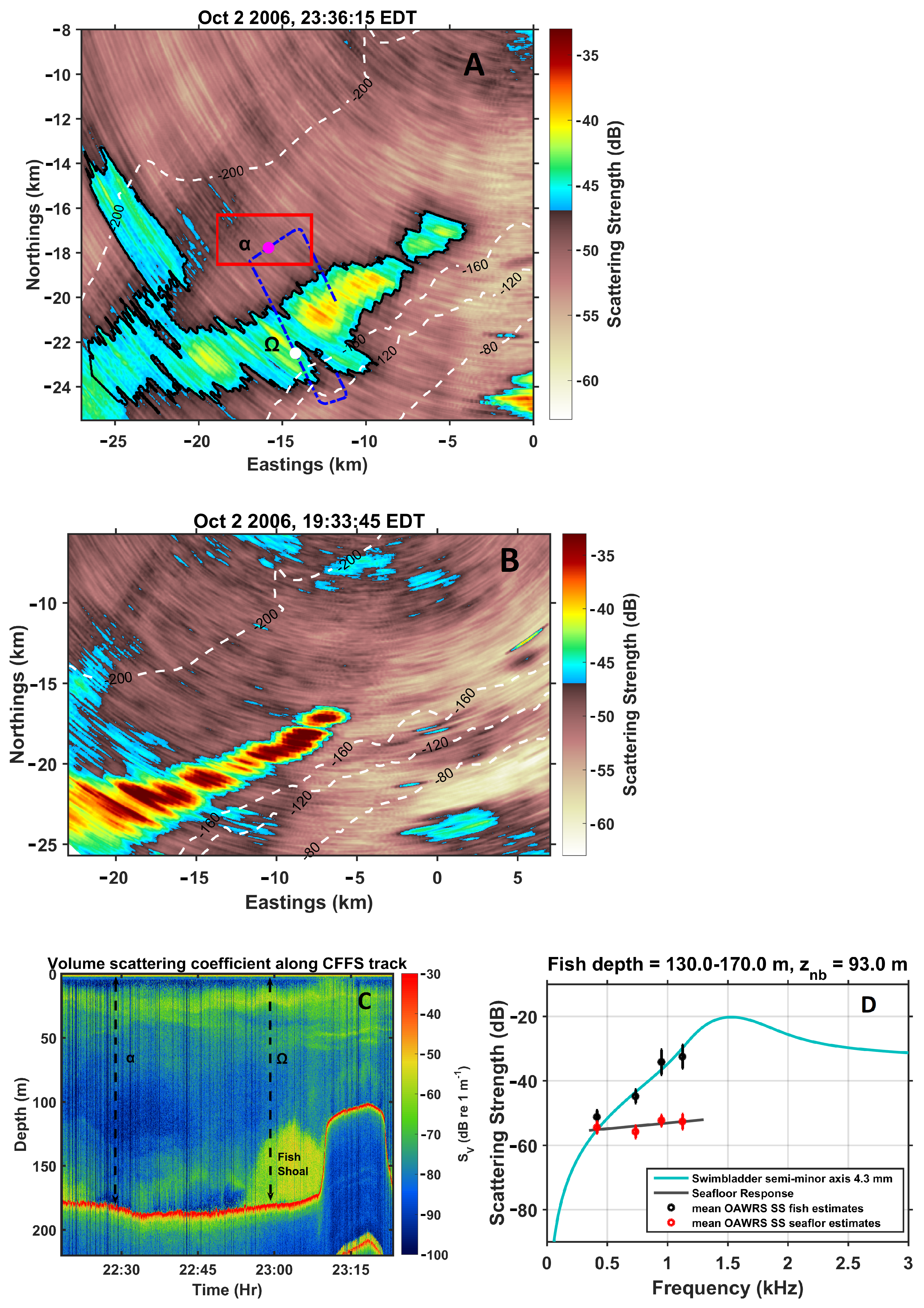
Here, we apply Neyman–Pearson hypothesis testing [24], which provides the highest probability of detection for a chosen false-alarm rate, to automatically distinguish fish from seafloor in wide-area multispectral OAWRS population density images.

First, we apply beamforming and matched filtering acoustic pressure field returns from an OAWRS transmission at a given center frequency and spatially charting their intensities to the spatial locations from which they were returned. Subsequently, the scattering strength for a given center frequency is determined at each spatial pixel by correcting for transmission loss over the OAWRS system resolution footprint following the approach described in References [3,6,7,12,17,28]. Examples of the resulting OAWRS image are shown in Figure 3A,B for a transmission with center frequency at 950 Hz, which is just below the expected swimbladder resonance peak for the swimbladder semi-minor axis length determined from trawl data (Figure 3C) as shown in Figure 3D [33]. Scattering strength images for the same times and locations were obtained for transmissions at four center frequencies—415, 735, 950 and 1125 Hz.

For a given OAWRS scattering strength image at a given center frequency, such as Figure 3A, taken to be training data, histograms are formed for scattering in regions with significant fish populations. These histograms represent the $H_1$ hypothesis of fish dominating scattering in a given region. The same is applied for regions with negligible fish populations, where the histograms represent the $H_0$ hypothesis of seafloor dominating scattering in a given region. The hypotheses are verified by: independent in situ conventional downward directed echo-sounder measurements as in Figure 3C; capture trawl; time-space variations in sequential OAWRS images consistent with dynamic fish migration; and frequency analysis as in Figure 3D, where scattering from fish swimbladder resonance exhibits a dramatic spectral dependence [3,6,7,12,17] not seen in seafloor scattering [16]. The process is repeated for all center frequencies. Both the multivariate $H_1$ and $H_0$ scattering strength probability density functions corresponding to these histograms are found to follow a Gaussian distribution by a Chi-Square goodness of fit test [34,35] with 5% of significance level as expected since the acoustic field can be described as a Circular Complex Gaussian Random variable (CCGR) [3,17,25,26,27].

The multivariate Gaussian probability density found for the $H_1$ hypothesis is then

$$\begin{array}{c}\hfill p_{H_1}({\mathit{SS}}_{\mathit{1}};{\mathit{\mu }}_1,{\Sigma }_1)=\frac{1}{{\left(2\pi \right)}^2{\left({\sigma }_{11}^2{\sigma }_{12}^2{\sigma }_{13}^2{\sigma }_{14}^2\right)}^{(1/2)}}exp\left(-\frac{1}{2}\left(\sum _{i=1}^4\frac{1}{{\sigma }_{1i}^2}{(S{S}_{1i}-{\mu }_{1i})}^2\right)\right).\end{array}$$

(1)

where ${\mathit{SS}}_{\mathbf{1}}$ is the random scattering strength vector for regions where fish scattering is dominant with four components $S_{1i}$ for $i=1,2,3,4$ corresponding to the four scattering strengths at OAWRS center frequencies 415, 735, 950, 1125 Hz. The mean of ${\mathit{SS}}_{\mathbf{1}}$ is ${\mathit{\mu }}_1$ with diagonal covariance ${\Sigma }_1$ that has variances ${\sigma }_{1i}$ determined from the training data. Similarly, for the $H_0$ hypothesis for regions with negligible fish scattering, the multivariate density is

$$\begin{array}{c}\hfill p_{H_0}({\mathit{SS}}_{\mathbf{0}};{\mathit{\mu }}_0,{\Sigma }_0)=\frac{1}{{\left(2\pi \right)}^2{\left({\sigma }_{01}^2{\sigma }_{02}^2{\sigma }_{03}^2{\sigma }_{04}^2\right)}^{(1/2)}}exp\left(-\frac{1}{2}\left(\sum _{i=1}^4\frac{1}{{\sigma }_{0i}^2}{(S{S}_{0i}-{\mu }_{0i})}^2\right)\right).\end{array}$$

(2)

where ${\mathit{SS}}_{\mathbf{0}}$ is the random scattering strength vector for regions where seafloor scattering is dominant, with four components $S_{0i}$ corresponding to scattering strengths at the four OAWRS center frequencies, with mean ${\mathit{\mu }}_0$ and variances ${\sigma }_{0i}$ determined from the training data.

To determine whether scattering at any spatial pixel in an OAWRS image is from fish or seafloor geology by Neyman–Pearson hypothesis testing, given measured scattering vector $\mathit{SS}$ at that pixel, the log of the likelihood ratio

$$\begin{array}{c}\hfill {\lambda }_{LR}=ln\left(\frac{P_{H_1}(\mathit{SS};{\mathit{\mu }}_1,{\Sigma }_1)}{P_{H_0}(\mathit{SS};{\mathit{\mu }}_0,{\Sigma }_0)}\right),\end{array}$$

(3)

is used [24]. In the log-likelihood ratio test, fish are taken to be present at a given spatial pixel if

$$\begin{array}{c}\hfill {\lambda }_{LR}\left(\mathit{SS}\right)>c_{critical},\end{array}$$

(4)

where $c_{critical}$ is chosen to yield a $1\%$ significance level of allowable false-positive detection rate.

3. Results

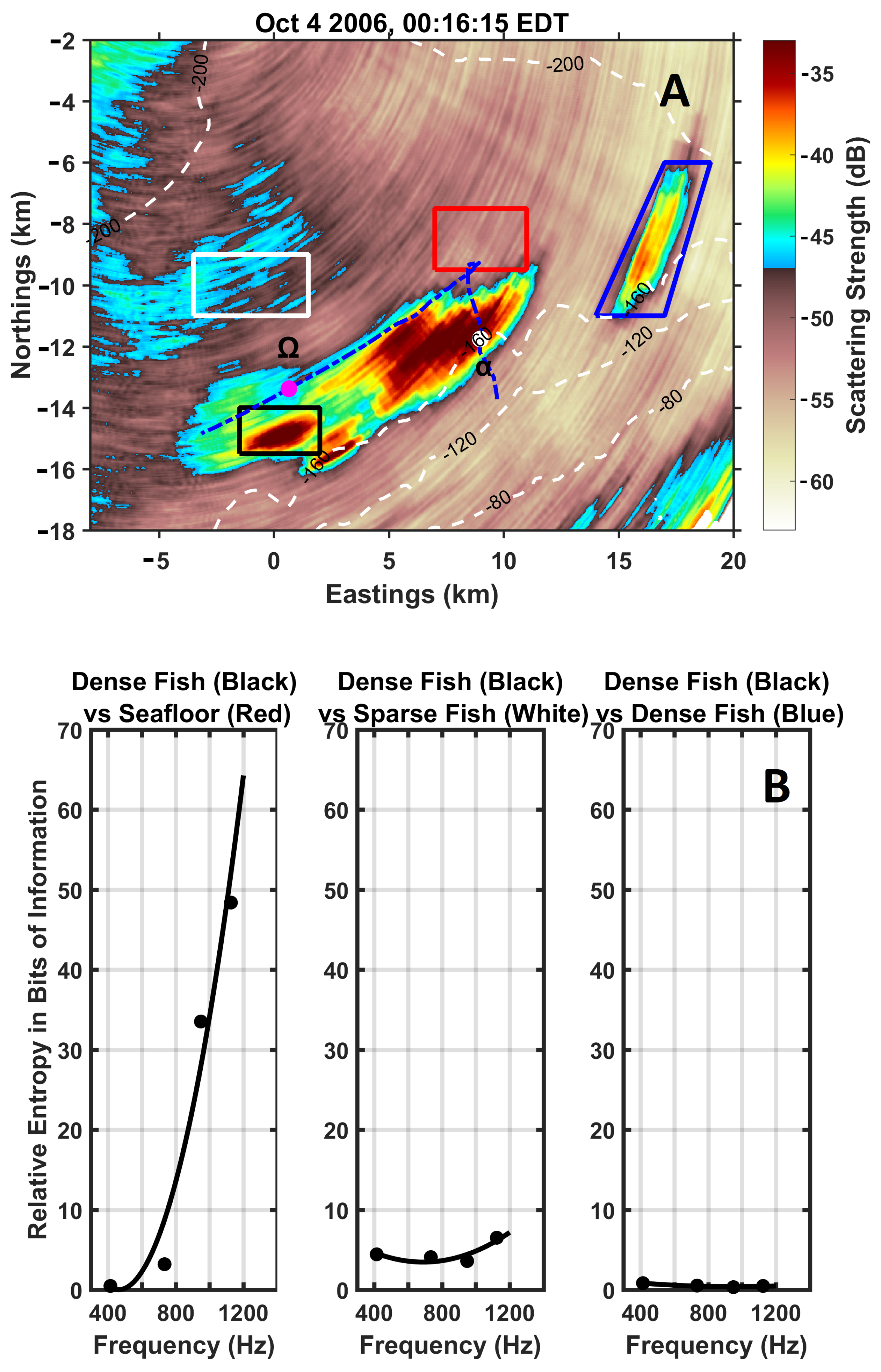
3.1. Automatic Optimal Discrimination of Fish from Seafloor Geology with Absolute Scattering Strength Levels

Neyman–Pearson hypothesis testing using the optimal decision rule of relation (4) is used to automatically evaluate whether a spatial pixel in multispectral OAWRS imagery is dominated by fish or seafloor geology. Test data $\mathit{SS}$ at pixels in Figure 3B are used, while training ${\mathit{SS}}_{\mathbf{0}}$ and ${\mathit{SS}}_{\mathbf{1}}$ data to determine the mean and covariances of the two hypotheses are from Figure 3A. The automatic classification results are as shown in Figure 4A, for pixels identified as primarily containing fish, and Figure 4B for regions dominated by seafloor scattering. These results correspond well with those determined from ground truth measurements, observation of temporal evolution, and manual spectral analysis.

Similarly, Neyman–Pearson hypothesis testing is applied for training data of Figure 5A, with ground truth data shown in Figure 5C,D, to test data in Figure 5B, leading to automatic pixel-by-pixel classification of fish-dominated versus seafloor-dominated scattering regions in Figure 6A,B. Again, the results correspond well with those determined from ground truth measurements, observation of temporal evolution and manual spectral analysis.

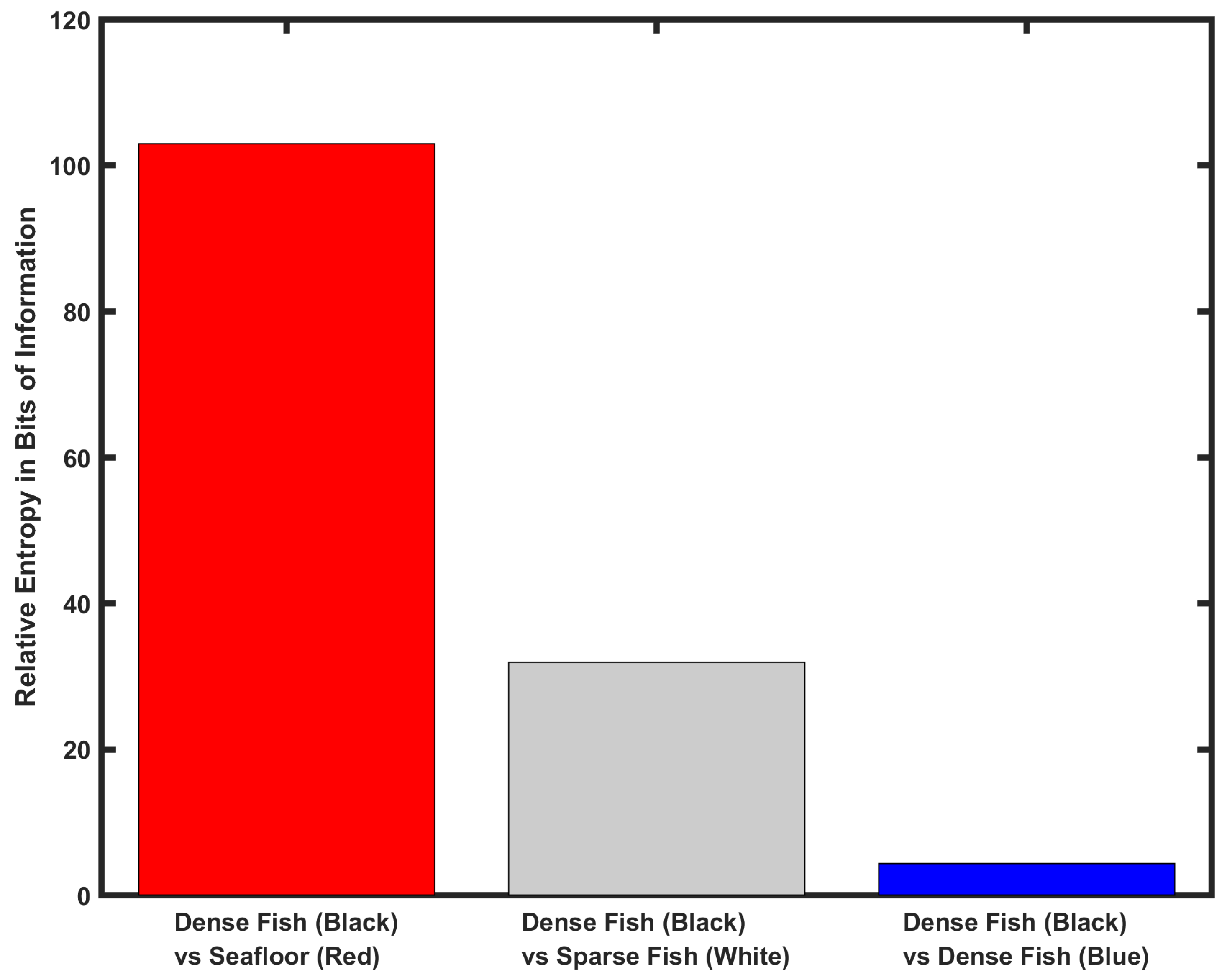
3.2. Automatic Optimal Discrimination of Fish from Seafloor Geology with Relative Spectral Dependencies

The approach of the previous section of using the absolute levels of scattering to distinguish fish from seafloor geology may restrict it to scenarios where the training data are very specifically tuned to specific environmental conditions where both fish shoals and seafloor geology have absolute scattering strength levels that are invariant. A more general approach is to use only the relative spectral dependencies of fish versus seafloor scattering in the hypothesis test which tends to be more invariant to changes in herring population density and seafloor depth, morphology and composition. This is accomplished by substituting ${\mathit{SS}}^{\prime }$ for $\mathit{SS}$ where ${\mathit{SS}}^{\prime }=\mathit{SS}-\frac{1}{N}{\sum }_{i=1}^{4}S{S}_i$ for $i=1,2,3,4$ scattering at four center frequencies. Similar offset adjustment by subtracting the mean scattering strength across frequency leads to ${\mathit{SS}}_{\mathbf{0}}^{\prime }$ and ${\mathit{SS}}_{\mathbf{1}}^{\prime }$, and all corresponding means and covariances of these random vectors as in Figure 7A,B. The modified, primed scattering strength vectors and their means and covariances are then substituted in Equations (1)–(3) and the relation (4) decision rule in place of the unprimed variables.

Neyman–Pearson hypothesis testing using the optimal decision rule of relation (4) is again used with the same critical value. Test data ${\mathit{SS}}^{\prime }$ at pixels in Figure 3B are used, while training data ${\mathit{SS}}_{\mathbf{0}}^{\prime }$ and ${\mathit{SS}}_{\mathbf{1}}^{\prime }$ for the two hypotheses are taken from Figure 3A. The automatic classification results are as shown in Figure 8A, for pixels identified as primarily containing fish, and Figure 8B for regions dominated by seafloor scattering. Similarly, Neyman–Pearson hypothesis testing is applied for training data of Figure 5A, with ground truth data shown in Figure 5C,D, to test data in Figure 5B, leading to automatic pixel by pixel classification of fish-dominated versus seafloor-dominated scattering regions in Figure 9A,B.

The results when only spectral dependencies are used in the classification are similar to those obtained when the absolute scattering strengths are used. Differences between the two approaches appear primarily at the edges of fish shoals. There, both spectral dependencies and levels of the mixed fish and seafloor returns differ from those of both the purely fish scattering Hypothesis 1 and the purely seafloor scattering Hypothesis 0 of the Neyman–Pearson test. Edges of shoals, however, comprise a small fraction of the area and total population of a shoal, especially when the scattering strength levels there are comparable with seafloor scattering.

4. Discussion

Since OAWRS may image many diverse environmental scatterers when sensing fish populations over wide areas, including those from seafloor geology, it is important to develop methods to efficiently identify pixels dominated by fish scattering in large data sets. Here, a method is developed and demonstrated to accomplish this task in an systematic, automatic and optimal manner given prior knowledge of the physical and statistical scattering properties of each type of scatterer. The particular prior knowledge employed here is for large herring shoals in their annual fall migration to spawning grounds on the northern flank of Georges Bank. The herring groups have been observed to migrate upslope near the seafloor from depths in the vicinity of 200-m to the very shallow regions for spawning with very similar scattering characteristics each day [7]. Strong variations in the spectral scattering response of the herring groups, which typically include or are in the vicinity of the swimbladder resonance peak, have been previously shown to be in the OAWRS spectral range of the present study [7,12,17]. Seafloor scattering in the vicinity has also been characterized and shown to have a very different and a far more constant or gradual spectral dependence over this OAWRS frequency range [16,36]. While the approach presented here is general, the training data are specific to herring shoals in the Northern Flank of Georges Bank during spawning migrations. For other regions and species, different training data or alternatively physical models will be necessary. With the current data, two approaches are employed. In the first, absolute scattering strengths measured are used to train and test the alternate Neyman–Pearson Hypotheses. In the second, only the normalized spectral dependence of scattering strength is used in the training and testing. The latter has advantages when fish populations densities or seafloor scatterers undergo large variations in absolute level, but maintain their spectral characteristics, making it more broadly applicable. Differences between the two approaches are found in regions where fish population densities are so low that their contribution to the total scattered field across frequency is similar to that of geologic seafloor scattering in the same pixel and neither hypothesis is best. For the large fish shoals of the present analysis, this is sometimes found at the shoal boundary, which comprises a very small part of the entire shoal area or population and so is not of critical importance. The creation of a third mixed hypothesis in this case is the subject of future work, with variable weighting for fish or seafloor that can be estimated from the data.

Another approach described in Appendix A, employing Kullback–Leibler divergence or relative entropy from Information Theory [37,38] is shown to also enable automatic discrimination of regions containing fish from those containing seafloor by use of their statistical scattering properties across sensing frequency. The approach shows that a significant difference, roughly two orders of magnitude larger in quantifiable bits of information, exists between regions dominated by fish versus seafloor scattering. To obtain robust divergences in bits, the approach of Appendix A is formulated purely in terms of empirical differences between the measured statistics of scattering between two regions containing a large number of independent pixels at each independent sensing frequency. As a result, it is not well-suited for discrimination at a single pixel, as is the Neyman–Pearson hypothesis testing approach presented in earlier sections.

5. Conclusions

Fish are optimally and automatically distinguished from seafloor geology at every pixel in multi-spectral Ocean Acoustic Waveguide Remote Sensing (OAWRS) images that instantaneously cover ecosystem scales. The optimality is attained by determining OAWRS scattering statistics of the competing hypotheses from prior data using the Neyman–Pearson decision rule, which provides the highest true positive detection rate possible for a given false alarm rate. Frequency-dependent scattering strengths of herring aggregations measured near their swimbladder resonance with OAWRS in the Gulf of Maine during the Autumn 2006 spawning season are used to develop and test the approach. Near swimbladder resonance, herring have a prominent spectral peak and sharp low frequency roll-off that distinguishes it from the mildly increasing to level frequency response of surrounding seafloor in the same frequency band. The likelihood function for herring and seafloor scattering are determined from the measured multi-spectral OAWRS imagery. The models are then applied to automate the discrimination of regions dominated by fish from those dominated by seafloor via the optimal Neyman–Pearson decision rule applied at each spatial pixel in instantaneous wide-area multi-spectral OAWRS imagery. The automated results are verified with ground-truth measurements of fish presence via local conventional echo-sounder measurements, capture trawls, analysis of time-space variations in scattered returns, as well as their spectral characteristics. The approach is found to be robust and should be broadly applicable.

The demonstrated pixel-by-pixel discrimination of fish from seafloor geology, optimized and automated over wide areas, has the potential to significantly impact the study of fish population dynamics, behavior and resource management. This is made even more compelling given current concerns about the effects of increased industrialization on the oceans and the effect of this and other modern pressures on the world’s fish populations.

Another approach, employing Kullback–Leibler divergence or relative entropy from Information Theory, is shown to also enable automatic discrimination of regions containing fish from those containing seafloor by use of their statistical scattering properties across sensing frequency. To garner robust divergences in quantifiable bits, however, this approach requires a large number of independent pixels in each region compared and so is less well suited to single-pixel discrimination than Neyman–Pearson hypothesis testing. It is also suboptimal in the sense that it does not provide the maximum true-positive detection rate for a given false-positive rate as does the Neyman–Pearson approach.

References

1. Gødo, O.R. Technology Answers to the Requirements Set by the Ecosystem Approach. In The Future of Fisheries Science in North America; Beamish, R.J., Rothschild, B.J., Eds.; Fish and Fisheries Series; Springer: Dordrecht, The Netherlands, 2009; Volume 31, pp. 373–403. [Google Scholar]
2. Nakken, O. Norwegian Spring-Spawning Herring & Northeast Arctic Cod: 100 Years of Research Management, 1st ed.; Tapir Academic Press: Trondheim, Norway, 2008. [Google Scholar]
3. Makris, N.C.; Ratilal, P.; Symonds, D.T.; Jagannathan, S.; Lee, S.; Nero, R.W. Fish Population and behavior revealed by instantaneous continental shelf-scale imaging. Science 2006, 311, 660–663. [Google Scholar] [CrossRef] [PubMed]
4. Overholtz, W.J.; Jech, J.M.; Michaels, W.I.; Jacobson, I.D.; Sullivan, P.J. Empirical comparisons of survey design in acoustic surveys of Gulf of Maine-Georges Bank Atlantic herring. J. Northwest Atl. Fish. Sci. 2006, 36, 127–144. [Google Scholar] [CrossRef]
5. Overholtz, W.J.; Friedland, K.D. Recovery of the Gulf of Maine herring (Clupea harengus) complex: Perspectives based on bottom trawl survey data. Fish. Bull 2002, 100, 593–608. [Google Scholar]
6. Jagannathan, S.; Bertsatos, I.; Symonds, D.; Chen, T.; Nia, H.; Jain, A.; Andrews, M.; Gong, Z.; Nero, R.; Ngor, L.; et al. Ocean Acoustic Waveguide Remote Sensing (OAWRS) of marine ecosystems. Mar. Ecol. Prog. Ser. 2009, 395, 137–160. [Google Scholar] [CrossRef]
7. Makris, N.C.; Ratilal, P.; Jagannathan, S.; Gong, Z.; Andrews, M.; Bertsatos, I.; Gødo, O.R.; Nero, R.W.; Jech, M. Critical population density triggers rapid formation of vast oceanic fish shoals. Science 2009, 323, 1734–1737. [Google Scholar] [CrossRef] [Green Version]
8. Makris, N.C.; Godø, O.R.; Yi, D.H.; Macaulay, G.J.; Jain, A.D.; Cho, B.; Gong, Z.; Jech, M.J.; Ratilal, P. Instantaneous areal population density of entire Atlantic cod and herring spawning groups and group size distribution relative to total spawning population. Fish Fish. 2019, 20, 201–213. [Google Scholar] [CrossRef] [Green Version]
9. Duane, D.; Cho, B.; Jain, A.D.; Gødo, O.R.; Makris, N.C. The Effect of Attenuation from Fish Shoals on Long-Range, Wide-Area Acoustic Sensing in the Ocean. Remote Sens. 2019, 11, 2464. [Google Scholar] [CrossRef] [Green Version]
10. Duane, D.; Gødo, O.R.; Makris, N.C. Quantification of Wide-Area Norwegian Spring-Spawning Herring Population Density with Ocean Acoustic Waveguide Remote Sensing (OAWRS). Remote Sens. 2021, 13, 4546. [Google Scholar] [CrossRef]
11. Duane, D.; Zhu, C.; Piavsky, F.; Godø, O.R.; Makris, N.C. The Effect of Attenuation from Fish on Passive Detection of Sound Sources in Ocean Waveguide Environments. Remote Sens. 2021, 13, 4369. [Google Scholar] [CrossRef]
12. Yi, D.H.; Gong, Z.; Jech, J.M.; Ratilal, P.; Makris, N.C. Instantaneous 3D Continental-Shelf Scale Imaging of Oceanic Fish by Multi-Spectral Resonance Sensing Reveals Group Behavior during Spawning Migration. Remote Sens. 2018, 10, 108. [Google Scholar] [CrossRef] [Green Version]
13. Wang, D.; Garcia, H.; Huang, W.; Tran, D.D.; Jain, A.D.; Yi, D.H.; Gong, Z.; Jech, J.M.; Gødo, O.R.; Makris, N.C.; et al. Vast assembly of vocal marine mammals from diverse species on fish spawning ground. Nature 2016, 531, 366–369. [Google Scholar] [CrossRef] [PubMed]
14. Overholtz, W.J. The Gulf of Maine-Georges Bank Atlantic herring (Clupea harengus): Spatial pattern analysis of the collapse and recovery of a large marine fish complex. Fish. Res. 2002, 57, 237–254. [Google Scholar] [CrossRef]
15. Love, R.H. A comparison of volume scattering strength data with model calculations based on quasisynoptically collected fishery data. J. Acoust. Soc. Am. 1993, 94, 2255–2268. [Google Scholar] [CrossRef]
16. Jain, A.D.; Ignisca, A.; Yi, D.H.; Ratilal, P.; Makris, N.C. Feasibility of Ocean Acoustic Waveguide Remote Sensing (OAWRS) of Atlantic Cod with Seafloor Scattering Limitations. Remote Sens. 2013, 6, 180–208. [Google Scholar] [CrossRef] [Green Version]
17. Gong, Z.; Andrews, M.; Jagannathanm, S.; Patel, R.; Jech, J.; Makris, N.C.; Ratilal, P. Low-frequency target strength and abundance of shoaling Atlantic herring (Clupea harengus) in the Gulf of Maine during the Ocean Acoustic Waveguide Remote Sensing 2006 Experiment. J. Acoust. Soc. Am. 2010, 127, 104–123. [Google Scholar] [CrossRef]
18. Chen, T.; Ratilal, P.; Makris, N.C. Temporal coherence after multiple forward scattering through inhomogeneities in an ocean waveguide. J. Acoust. Soc. Am. 2008, 124, 2812–2822. [Google Scholar] [CrossRef] [Green Version]
19. Yi, D.H.; Makris, N.C. Feasibility of Acoustic Remote Sensing of Large Herring Shoals and Seafloor by Baleen Whales. Remote Sens. 2016, 8, 693. [Google Scholar] [CrossRef] [Green Version]
20. Cho, B.; Makris, N.C. Predicting the Effects of Random Ocean Dynamic Processes on Underwater Acoustics Sensing and Communication. Sci. Rep. 2020, 10, 4525. [Google Scholar] [CrossRef] [Green Version]
21. Schinault, M.E.; Seri, S.G.; Radermacher, M.K.; Mohebbi-Kalkhoran, H.; Zhu, C.; Makris, N.C.; Ratilal, P. Development of a large-aperture 160-element coherent hydrophone array system for instantaneous wide area ocean acoustic sensing. In Proceedings of the OCEANS 2022, Hampton Roads, VA, USA, 17–20 October 2022. [Google Scholar]
22. Mohebbi-Kalkhoran, H.; Schinault, M.E.; Makris, N.C.; Ratilal, P. Integrated computing system for real-time data processing, storage, and communication for large aperture 160-element coherent hydrophone array. In Proceedings of the OCEANS 2022, Hampton Roads, VA, USA, 17–20 October 2022. [Google Scholar]
23. Ratilal, P.; Seri, S.G.; Mohebbi-Kalkhoran, H.; Zhu, B.; Schinault, M.E.; Radermacher, M.K.; Makris, N.C. Continental Shelf-scale Passive Ocean Acoustic Waveguide Remote Sensing of Marine Ecosystems, Dynamics and Directional Soundscapes: Sensing Whales, Fish, Ships and other Sound Producers in near Real-Time. In Proceedings of the OCEANS 2022, Hampton Roads, VA, USA, 17–20 October 2022. [Google Scholar]
24. Kay, S.M. Fundamental of Statistical Signal Processing—Vol. 2 Detection Theory, 1st ed.; McGraw-Hill: Providence, RI, USA, 1993; pp. 60–93. [Google Scholar]
25. Andrews, M.; Chen, J.M.; Ratilal, P. Empirical dependence of acoustic transmission scintillation statistics on bandwidth, frequency, and range on New Jersey continental shelf. J. Acoust. Soc. Am. 2009, 125, 111–124. [Google Scholar] [CrossRef] [Green Version]
26. Makris, N.C. A foundation for logarithmic measures of fluctuating intensity in pattern recognition. Opt. Lett. 1995, 20, 2012–2014. [Google Scholar] [CrossRef]
27. Makris, N.C. The effect of saturated transmission scintillation on ocean acoustic intensity measurements. J. Acoust. Soc. Am. 1996, 100, 769–783. [Google Scholar] [CrossRef]
28. Jain, A.D.; Makris, N.C. Maximum Likelihood Deconvolution of Beamformed Images with Signal-Dependent Speckle Fluctuations from Gaussian Random Fields: With Application to Ocean Acoustic Waveguide Remote Sensing (OAWRS). Remote Sens. 2016, 8, 694. [Google Scholar] [CrossRef] [Green Version]
29. Becker, K.; Preston, J. The ONR five octave research array (FORA) at Penn State. In Proceedings of the Oceans 2003, Celebrating the Past…Teaming Toward the Future. (IEEE Cat. No.03CH37492), San Diego, CA, USA, 22–26 September 2003; Volume 5, pp. 2607–2610. [Google Scholar]
30. Wang, D.; Ratilal, P. Angular Resolution Enhancement Provided by Nonuniformly-Spaced Linear Hydrophone Arrays in Ocean Acoustic Waveguide Remote Sensing. Remote Sens. 2017, 9, 1036. [Google Scholar] [CrossRef] [Green Version]
31. Makris, N.C.; Avelino, I.Z.; Menis, R. Deterministic reverbation from ocean ridges. J. Acoust. Soc. Am. 1994, 97, 3547–3574. [Google Scholar] [CrossRef]
32. Ratilal, P.; Lai, Y.; Symonds, D.; Ruhlmann, I.A.; Preston, J.R.; Scheer, E.K.; Garr, M.T.; Holland, C.W.; Goff, J.A.; Makris, N.C. Long range acoustic imaging of the continental shelf environment: The Acoustic Clutter Reconnaissance Experiment 2001. J. Acoust. Soc. Am. 2005, 117, 1977–1998. [Google Scholar] [CrossRef] [Green Version]
33. Love, R.H. Resonant acoustic scattering by swimbladder-bearing fish. J. Acoust. Soc. Am. 1978, 64, 571–580. [Google Scholar] [CrossRef]
34. Pearson, K. On the criterion that a given system of deviations from the probable in the case of a correlated system of variables is such that it can be reasonably supposed to have arisen from random sampling. Philos. Mag. 1900, 50, 157–175. [Google Scholar] [CrossRef] [Green Version]
35. Kay, S.M. Fundamental of Statistical Signal Processing—Vol. 1 Estimation Theory, 1st ed.; McGraw-Hill: Providence, RI, USA, 1993. [Google Scholar]
36. Kaklamanis, E. Spectral Discrimination of Fish Shoals from Seafloor in the Gulf of Maine during the Ocean Acoustic Waveguide Remote Sensing (OAWRS) 2006 Experiment. Ph.D. Thesis, Massachusetts Institute of Technology (MIT), Cambridge, MA, USA, 2021. [Google Scholar]
37. Kullback, S. Information Theory and Statistics; John Wiley and Sons: Hoboken, NJ, USA, 1959. [Google Scholar]
38. Kullback, S.; Leibler, R.A. On information and sufficiency. Ann. Math. Stat. 1951, 22, 79–86. [Google Scholar] [CrossRef]
Figure 1. Instantaneous areal coverage of a single OAWRS transmission in the Gulf of Maine 2006 experiment shown over bathymetry. A region of 100 km in diameter (red circle) and roughly 8000 square kilometers is surveyed within 75 s by OAWRS. Widely spaced line transects of the concurrent National Marine Fisheries Service (NMFS) two-week survey. NMFS used a downward directed echo-sounder to sense within a few horizontal meters of the research vessel track shown in yellow. Yellow NMFS survey tracks are not shown within the OAWRS circle to avoid visual clutter, but extended there along the lines shown.
Remotesensing 15 00437 g001
Figure 2. OAWRS receiving array system used during the Gulf of Maine 2006 Experiment [7]. The towed horizontal receiving array and OAWRS vertical source array were separately deployed from two research vessels for bistatic measurements.
Remotesensing 15 00437 g002
Figure 3. Discrimination of fish from seafloor scattering regions by Neyman–Pearson hypothesis testing. (A) OAWRS 950 Hz scattering strength measured on 3 October, at 18:18:45 EDT, with bathymetric contours (dashed white lines) dominated by scattering from massive fish shoal extending for roughly 30 km (training data within black contour) and seafloor geology (training data within red contour). Coordinate origin is located at the source array location. Data from these respective contoured regions are used to determine the likelihood functions. (B) OAWRS 950 Hz scattering strength image containing fish and seafloor scattering at various pixels measured on 3 October, at 19:21:15 EDT to be sorted as test data using Neyman–Pearson decision rule. (C) Time-depth profile of fish volumetric density (fish/m3) measured by high-frequency downward-directed echo-sounding, along the blue line-transect of NOAA FRV Delaware II research vessel through the shoal shown in (A). White dashed vertical lines correspond to Delaware II transect start α and end Ω points. (D) Measured scattering strength ( SS ) versus frequency for four OAWRS center frequencies for black-bounded region in (A) shows excellent least-square fit with Love-model frequency response for herring with swimbladder semi-minor mean of 4.9 mm, with standard deviation typically within + / 30% of semi-minor axis mean. Scattering strength versus frequency of red-bounded region in (A) show excellent correspondence with seafloor scattering [16].
Remotesensing 15 00437 g003
Figure 4. Each pixel in Figure 3B measured on 3 October, 19:21:15 EDT is classified as being dominated by fish or seafloor scattering with the likelihood ratio test of Equation (3). (A) Pixels classified as dominated by fish scattering. (B) Pixels classified as dominated by seafloor scattering.
Remotesensing 15 00437 g004
Figure 5. Same as Figure 3 except OAWRS scattering strength in (A) is measured on 2 October 23:36:15 EDT and (B)—on 2 October 19:33:45 EDT, echosounder tracks in (C) are shown with blue line in (A) and scattering strength versus frequency for fish and seafloor in (D) are within black and red contours, respectively.
Remotesensing 15 00437 g005
Figure 6. Each pixel in Figure 5B measured on 2 October 19:33:45 EDT is classified as being dominated by fish or seafloor scattering with the likelihood ratio test of Equation (3). (A) Pixels classified as dominated by fish scattering. (B) Pixels classified as dominated by seafloor scattering.
Remotesensing 15 00437 g006
Figure 7. Relative scattering strength versus frequency for fish and seafloor after subtracting instantaneous average scattering strength over frequency at each pixel comprising different relative spectral dependencies measured on (A) 3 October 18:18:45 EDT and (B) 2 October 23:36:15 EDT.
Remotesensing 15 00437 g007
Figure 8. Each pixel in Figure 3B measured on 3 October 19:21:15 EDT is classified as being dominated by fish or seafloor scattering with the log-likelihood ratio test of Equation (3) using relative frequency responses obtained by subtracting the mean instantaneous average scattering strength across frequency at each pixel. (A) Pixels classified as dominated by fish scattering. (B) Pixels classified as dominated by seafloor scattering.
Remotesensing 15 00437 g008
Figure 9. Same as Figure 8 except OAWRS scattering strength is measured on 2 October 19:33:45 EDT. Each pixel in Figure 5B is classified as being dominated by fish or seafloor scattering using relative frequency responses obtained by subtracting the mean instantaneous average scattering strength across frequency at each pixel. (A) Pixels classified as dominated by fish scattering. (B) Pixels classified as dominated by seafloor scattering.
Remotesensing 15 00437 g009
Disclaimer/Publisher’s Note: The statements, opinions and data contained in all publications are solely those of the individual author(s) and contributor(s) and not of MDPI and/or the editor(s). MDPI and/or the editor(s) disclaim responsibility for any injury to people or property resulting from any ideas, methods, instructions or products referred to in the content.