Article

Dry Matter Yield and Nitrogen Content Estimation in Grassland Using Hyperspectral Sensor

1
Agrosystems Research Institute, Wageningen University & Research, 6700 AA Wageningen, The Netherlands
2
KUBOTA Corporation, 1-11 Takumi-cho, Sakai-ku, Sakai 590-0908, Osaka, Japan
3
Livestock and Environment, Wageningen Livestock Research Institute, Wageningen University & Research, 6708 WD Wageningen, The Netherlands
*
Author to whom correspondence should be addressed.
Remote Sens. 2023, 15(2), 419; https://doi.org/10.3390/rs15020419
Submission received: 21 October 2022 / Revised: 30 December 2022 / Accepted: 7 January 2023 / Published: 10 January 2023
(This article belongs to the Special Issue Remote Sensing of Agro-Ecosystems)

Abstract

:
Estimation of Dry Matter Yield (DMY) and Nitrogen Content (NC) in forage is a big concern for growers. In this study, an estimation model of DMY and NC using Visible and Near Infrared (V-NIR) spectroscopy was developed. An adequate number of grass samples (5078) of perennial ryegrass (Lolium perenne), collected from Dutch grassland in 2019 and 2020 were sensed with a hyperspectral sensor, while grass height was recorded in situ by an ultrasonic sensor mounted on a tractor. The samples were treated with Artificial Intelligence (AI) techniques. PCA based feature selection was applied first, revealing that visible green wavelength (around 500 nm) and red edge wavelength (around 700 nm) were enough to express the overall variability of the dataset. Then, Feature Importance analysis of Random Forest Regressor showed that NIR wavelengths (around 910, 960 and 990nm) were the most sensitive in DMY estimation, while red edge (around 710 nm) and visible orange wavelengths (around 610 nm) were the most related to NC estimation. Finally, SHAP (SHapley Additive exPlanations) analysis was applied to the Random Forest estimation models, resulting in the visualization of wavelength selection, thus assisting in the interpretation of the results and the intermediate processes. Overall, this method can lead to the reduction of the number of wavelengths to be measured in the field and thus, to the possible development of a low cost hyperspectral sensor for the above purposes.

1. Introduction

Grassland research is one of the indispensable studies in Europe, given that approximately 34% of agricultural land in the European Union is regarded as permanent grassland [1]. In the Netherlands, United Kingdom, and Ireland, grassland covers 54%, 72%, and 92% of land, respectively [2]. Grassland is not only considered as a need for animal products, but also plays a vital role in the environment, such as minimizing the damage of erosion and flood [3]. Although the multifunctional traits of grassland are well-known in the context of the ecosystem, the area of grassland has declined in Europe over the decades due to land use change, which is related to political transformation and environmental concerns (livestock, methane emission), and intensification [4]. In this context, it is important to find a strategy to improve productivity within the limited grassland area to provide animal products in a more efficient way [3,5].
According to previous studies [6,7], nitrogen use efficiency in grassland is very limited, because more than 50% of the N applied is not assimilated by plants. Furthermore, environmental awareness of high nitrogen input through manure and chemical fertilizers is very important since it could potentially cause deterioration of groundwater and surface water [7].
Another aspect is that in grassland farming assessing Dry Matter yield (DMY) and nitrogen content (NC) is a big concern for farmers. DMY is not only directly related to the amount of pasture but also utilized for post processes such as tedding, raking, baling, or making silage in the form of DMY within a harvested pasture. NC is strongly related to crude protein content within the pasture, and crude protein is a key factor for the total intake and digestion of cattle.
In order to monitor DMY or NC, several approaches have been developed. In general, grass samples are collected in the field and sent to a laboratory to be analyzed by chemical methods. However, this is usually costly and takes time.
There have been studies to estimate DMY and NC using near infra-red spectroscopy. In this area of research, it is important to identify the wavelengths that contribute to the estimation, which will lead to the development of low-cost sensors [8,9,10,11]. One common method for this purpose is principal component analysis (PCA) [12,13,14]. For each feature, the contribution value to the principal components is calculated by PCA. Based on this contribution value, dominant features, i.e., bands in this case, can be selected. Another method for band selection is random forest regressor [15]. Band selection is performed according to the importance of the features calculated by the structure of random forest regressor. Other methods, genetic algorithm (GA), phased regression (PHR), or principal component regressor are also used [16,17]. However, with the above methods, feature importance is expressed as an absolute value, no matter if the correlation is positive or negative. If the transition of the importance of wavelength can be analyzed more precisely, such as when the importance becomes high, low, or even negative, the wavelength for sensors can be selected more reasonably. In addition, it could be useful for a deeper understanding of measured values or results of prediction models, and also for data pre-processing and designing models themselves.
For further utilization of near-infrared spectroscopy in grassland management, this research addresses the improvement of the estimation accuracy of DMY and NC and develops a feature selection method to determine the dominant wavelength. Combining hyperspectral absorbance data with other field measurements, specifically the plant height sensor, focuses on improving the accuracy of DMY and NC estimation. In addition, for more detailed wavelength analysis, several techniques to identify wavelengths which contribute for estimating DMY and NC of pasture are examined. Reducing the number of wavelengths to be measured by hyperspectral sensor might lead to the development of lower cost sensors. Each specific methodology is discussed in following sections.

2. Materials and Methods
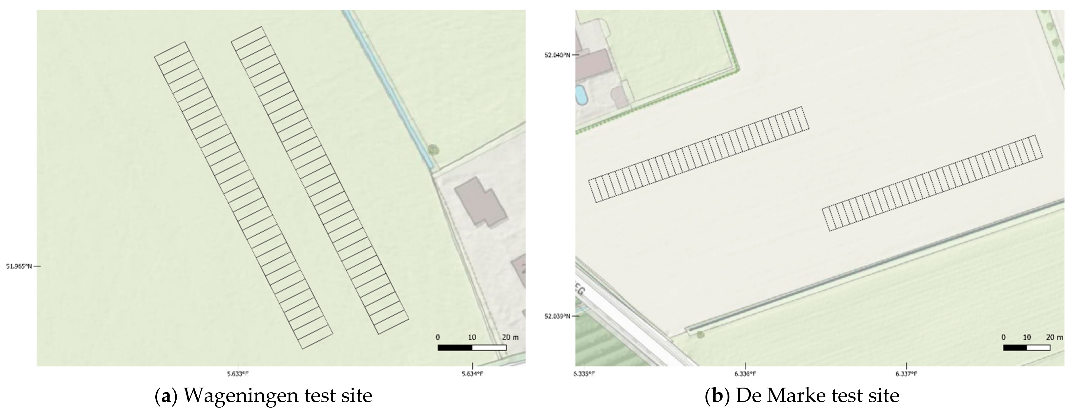
2.1. Study Site

An experiment of grassland fields was conducted in the 2019 and 2020 crop seasons from May to October. The dominant grass vegetation was Lolium perenne, one of the perennial ryegrasses widely grown as pasture for livestock not only in the Netherlands but also around the world. The study sites were in Wageningen (51.964°N–51.966°N, 5.632°E–5.634°E) and De Marke (52.040°N–52.039°N, 6.355°E–6.338°E), both a part of The Netherlands. Both fields have 64 plots and each plot has an area of 10 m × 3 m, as shown in Figure 1. The soil type of the field in Wageningen is clay soil, whereas that in De Marke is sandy soil. Annual precipitation (mm/h), minimum temperature (°C), maximum temperature (°C), and average temperature (°C) in Wageningen throughout 2019 and 2020 are 2.3, 7.4, 15.2, and 11.1, respectively, while their statistics in De Marke are 2.2, 7.4, 15.0 and 11.0, respectively.
In Wageningen, harvesting and data acquisition were performed five times in 2019 (30th April, 17th June, 29th July, 3rd September and 29th October) and four times in 2020 (6th May, 22nd June, 11th September and 15th October). In De Marke, harvesting and data acquisition were performed four times in 2019 (13th May, 24th June, 2nd September and 21st October), and five times in 2020 (6th May, 8th June, 17th July, 16th September and 26th October)
In 2019, 32 out of 64 plots were unfertilized, and the remaining 32 fields were fertilized by applying nitrogen. Plots in Wageningen were fertilized in amounts of 140 kg/ha, 100 kg/ha, 60 kg/ha and 40 kg/ha from the 1st cut to the 4th cut, for a total of 340 kg/ha. Plots in De Marke were fertilized in amounts of 140 kg/ha, 90 kg/ha, 81 kg/ha, 54 kg/ha, and 40 kg/ha from the 1st cut to the 5th cut, for a total of 405 kg/ha. On the other hand, different fertilizing methods were employed in order to artificially create different growing conditions in 2020. Specifically, 8 out of 64 plots were unfertilized, 28 plots were equally fertilized, which means the same way as the fertilizing scheme in 2019, and the remaining 28 plots were fertilized in different ways in order to artificially create different growing conditions. For the remaining 28 plots, based on the NC from grass in 2019, more fertilizer was applied to the plots that had more nitrogen.

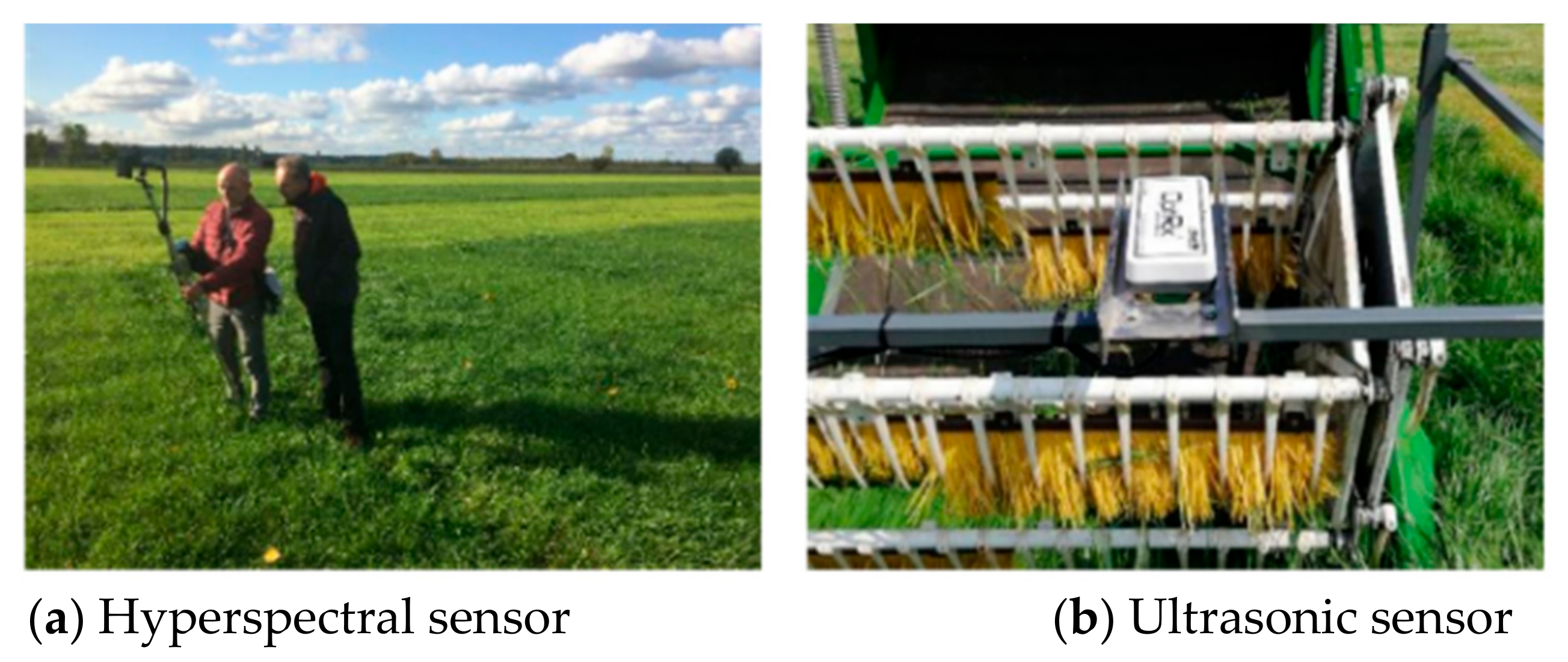
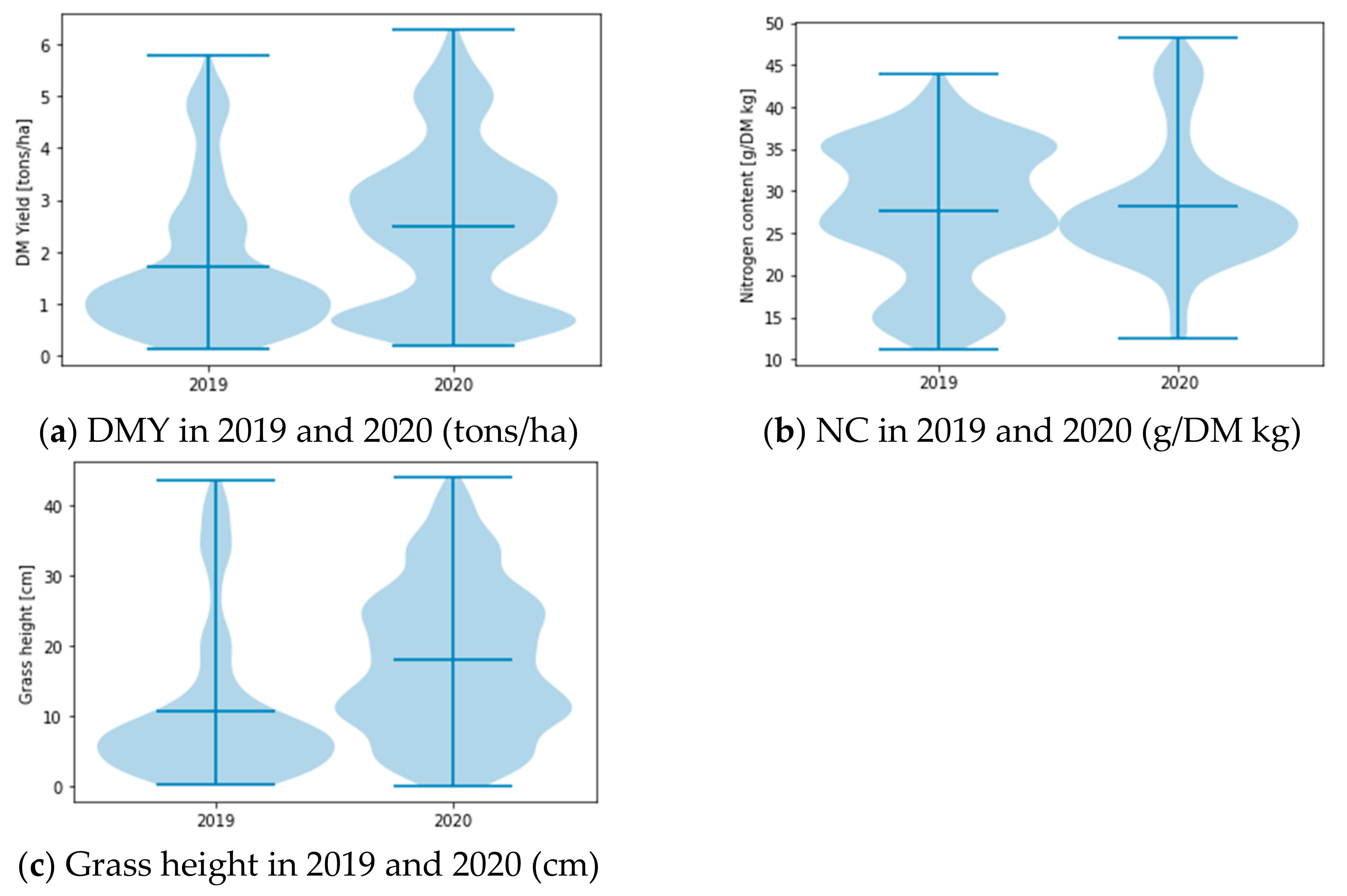
2.2. Data Collection

In this field experiment, the grass was cut four to five times a year. All plots per location were harvested on the same day using a forage harvester from Haldrup GmbH “https://www.haldrup.net/ (accessed on 9th January 2023)” specially designed for this experiment. The harvesting area was 10 × 1.5 m inside each plot.
First, the weight of harvested fresh grass on each plot was measured. After assessing the fresh weight per plot, approximately 300 to 500 g of grass was randomly sampled in order to determine the DMY. These samples were dried for 48 h at 70 °C and homogenized by grinding in a 0.5 mm mill. Samples were taken from these materials to assess the remaining moisture content by drying at 105 °C. Samples were taken from the remaining materials to assess the total NC by the method of “digestion H2SO4-H2O2-Se; SFA-Nt/Pt”.
Grass height was measured with a Pasture Reader “http://pasturereader.com.au/ (accessed on 9th January 2023)” which is placed in front of the forage harvester. The Pasture Reader is a sensor that measures the height and the density of the grasses ultrasonic waves. Plant height was measured weekly for each plot.
Before each harvest, crop reflectance was measured by Tec5 HandySpec Field equipment “https://tec5.com/en/products/nir-systems/ (accessed on 9th January 2023)”. It is a spectroscopic sensor system that measures the light absorption of plants or soil in specific wavelength bands based on near-infrared spectroscopy. Measurements are independent of atmospheric influence because of permanent referencing of the ambient light (upper sensor). The spectral data can be used to evaluate biomass, leaf area and nitrogen status. The instrument measures incoming and reflected light simultaneously. The covered wavelength is 400–1000 nm with a spectral resolution of 10 nm. The sensor is held manually at a height of approx. 1.8 m above the top of the canopy and pointed directly downward. The field of view of the sensor is ±25°, which results in a measurement of roughly 0.5 m2 of the crop. The sensors used for data collection are shown in Figure 2. The methods and parameters used to measure grass samples from each harvesting area are summarized in Table 1.
Measurements were taken only when the crop was dry. Measurements were taken between 10:00 am and 4:00 pm in order to avoid low solar angles. The operator faced the sun to prevent shading the object. Measurements were made on six different spots within the harvest area of each plot.
Throughout two years of data collection, 2434 and 2644 measurements were collected during harvest in 2019 and 2020, respectively. Histograms of measured data are shown in Figure 3.
DMY and grass height in 2020 were higher than in 2019. There was a lack of precipitation during the crop season in 2020, but optimization of water supply in 2020 with a dripping irrigation system, which could have caused a higher yield. Accumulated rainfall in the pasture growing season in 2019 and 2020 was 474 mm and 411 mm, respectively, in Wageningen, and 480 mm and 425 mm, respectively, in De Marke, i.e., 13% and 11% less, respectively, in 2020. In Wageningen, no irrigation was applied in 2019, while the amount of irrigation in 2020 was 12 mm on 20th May, 15 mm on 27th May, and 15 mm on 10th August, totaling 42 mm. In De Marke, the amount of irrigation in 2019 was 27 mm on 11th July and 34 mm on 31st July, totaling 61 mm, while irrigation in 2020 was 17 mm on 17th April, 18 mm on 13th May, 21 mm on 4th June, 17 mm on 1st August, 22 mm on 7th August, 21 mm on 15th August and 12 mm on 20th September, totaling 129 mm. Here, the growing season was assumed to be from 1st April to 31st October.

2.3. Data Analysis

Using the measurement data collected as the described in previous section, estimation model of DMY and NC is developed. In this section, the methods of the model development and its analysis are explained.

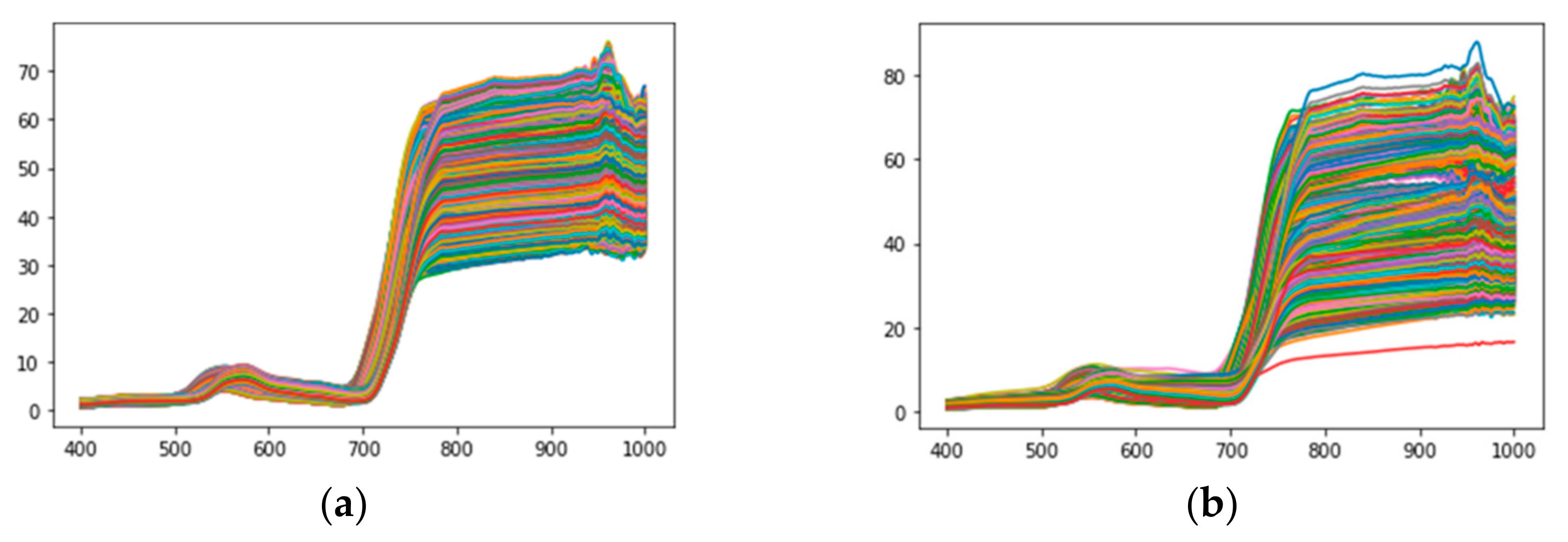
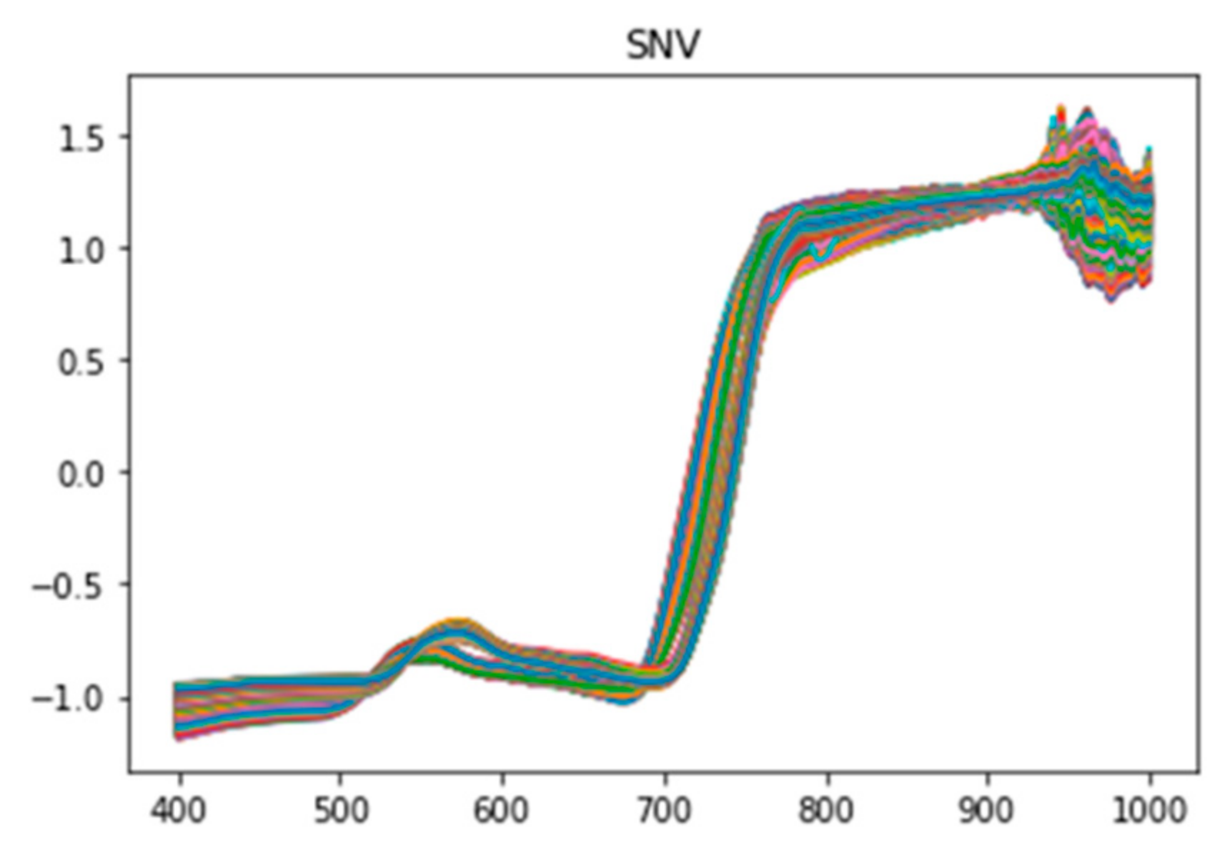
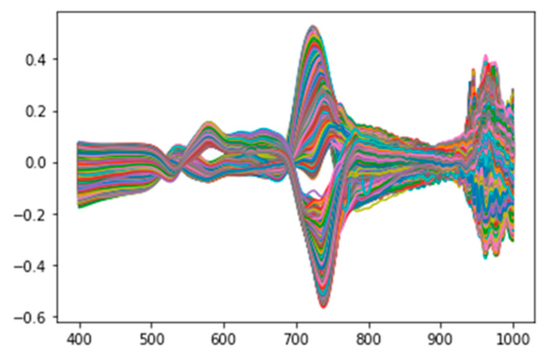
2.3.1. Data Pre-Process

In general, measurement data of living organisms such as plants contain a lot of noise. Therefore, pre-processing of the data to create clean data is indispensable for the application of multivariate analysis, artificial intelligence (AI), etc. to obtain robust and reliable results. For this purpose, the data pre-process procedure shown in Figure 4 was applied.
Details of each procedure are explained in Appendix A. By pre-processing, noise and outliers are removed, the difference in the absolute value of each variable is smoothed out and the useful variables are emphasized, which in turn leads to good data analysis results.

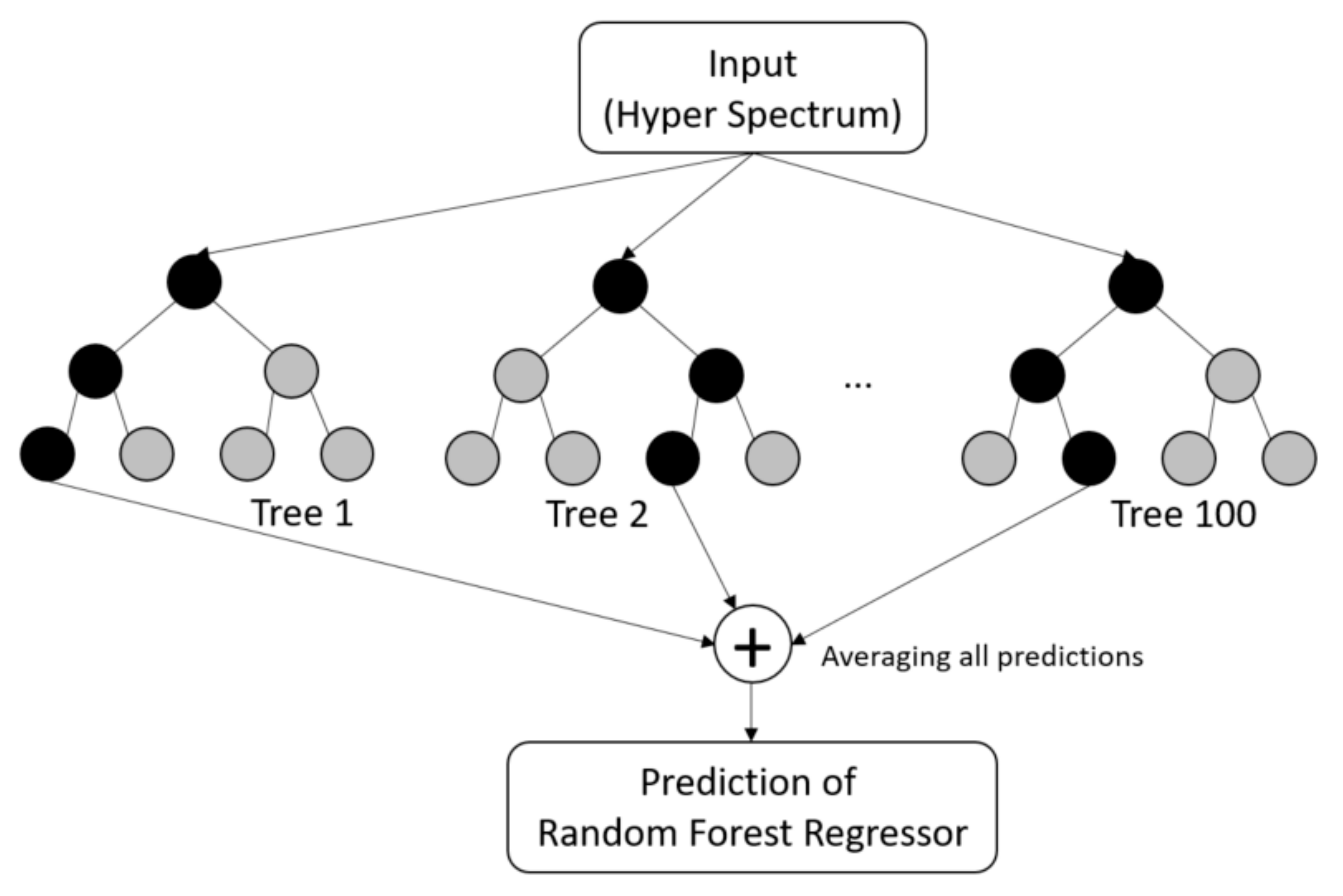
2.3.2. Random Forest Regressor

Random forest regressor [14] is used to build a prediction model of DMY and NC of grass from hyperspectral measurement data. Random forest regressor is a kind of supervised learning algorithm for regression. It uses an ensemble learning method, which combines the output (prediction) from multiple decision trees.
Random forest regressor has less computational costs and it is easier to understand the output since it is based on a decision tree algorithm. The structure of the random forest regressor is shown in Figure 5.
For the purpose of building an estimation model, PLS (partial least squares regression) [15,16,17], MPLS (modified partial least squares regression) [18,19], PCR (principal component regression), and GA [13,15] are generally used in related research. Compared to them, fewer parameters of random forest regressor (number of estimators and max depth of each tree) are also one of the advantages.
“Number of estimators” and “max depth” are set to “100” and “none”, respectively. When “max depth” is “none,” nodes are expanded until all leaves become pure. Since the random forest-based approach is known to be parameter robust [20], the default value of 100 for the number of trees parameter of the software library “scikit-learn” described in the following section were applied.
By using random forest regressor, feature importance which indicates the magnitude of the effect of each feature (i.e., wavelength) on the estimation, can be calculated as the mean and standard deviation of accumulation of the impurity decrease within each tree.

2.3.3. X-Loading Analysis

Loadings in principal component analysis (PCA) are interpreted as the coefficients of the linear combination of the initial variables from which the principal components (PCs) are constructed. Loadings are also known as the values that represent the contribution of each variable (i.e., the importance of each variable) [7,21]. Therefore, X-Loadings analysis can reveal the important variables of principal components (in this case, the wavelength band), which explains the variance of the measured grass samples well.

2.3.4. SHAP Analysis

SHAP (shapley additive explanations) analysis is a method to calculate the contribution rate of each feature of each input value to the output of recognition or regression models [22]. The SHAP value is calculated by the following formula and expressed by each input value, that is, the absorbance magnitude of each wavelength band in this document. Hence, it is possible to explain why the prediction was made for the predicted value. For example, SHAP can visualize not only the importance of features that can be visualized by conventional methods such as PCA, but also the contribution of each data at the level of each variable and the positive or negative effect between features and output. More importantly, SHAP analysis is applicable to all AI models besides random forest regressor. Therefore, it is a means to solve the disadvantage of AI, which is considered to be one of the biggest disadvantages of being a black box.
When given the input x and trained model f   , the model f   is approximated with model g   to explain the contribution rate of each input variable. Model g   is defined as the following Equation (1):
g z = ϕ 0 + i = 1 M ϕ i z i
where ϕ i is the contribution of i   -th variable of input x   and z i indicates 1 when i   -th variable is observed, otherwise 0. More details are explained in [22].
For the purpose of investigating the importance of features, feature selection methods such as PCA, random forest regressor, GA or phased regression (PHR) [12,13] are commonly used. GA is an algorithm that uses the evolutionary mechanism of organisms to evolve into highly superior individuals through crossover or mutation, and PHR is a model that performs stepwise regression. However, these methodologies only show the importance of features as an absolute value, no matter if the correlation is positive or negative. By using SHAP analysis, both strong positive and negative values can be calculated as positive or negative SHAP values. Besides, how each feature of each input value affects the output values can be calculated and visualized.

2.4. Computational Environment

All the computations in this paper were performed in the virtual environment of Python 3.7.1, which is built on Cluster Computing Environment of Wageningen University & Research. The operation system is Scientific Linux 7.9. Assigned CPU and memory to the virtual environment were one core and 8 GB, respectively.
For the purpose of statistical analysis of measurement data, the following packages were used:

3. Results & Discussion

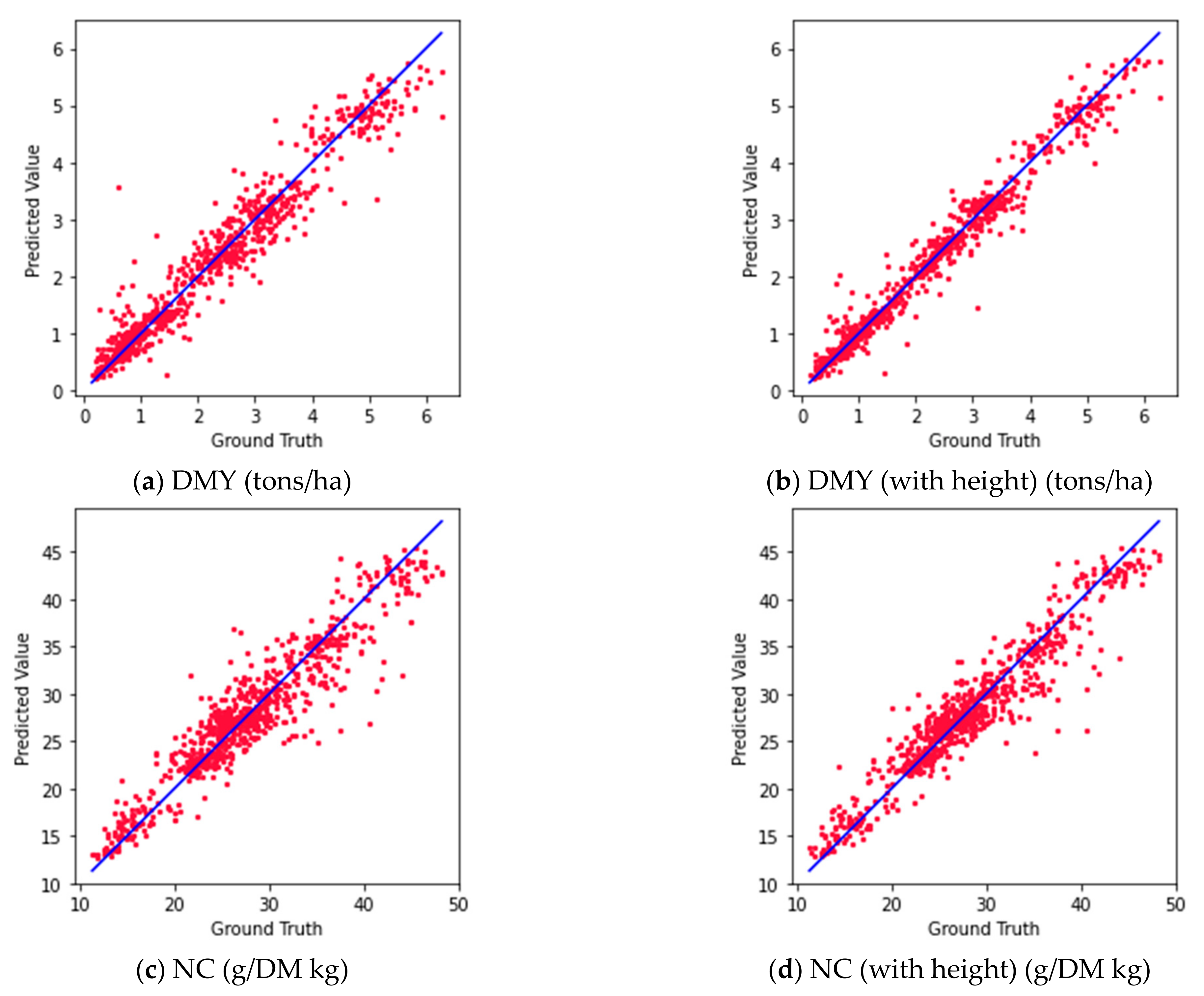
3.1. Estimation of DMY and NC

In this paper, random forest regressor was used as one of the AI models, as is simple and easy to understand its structure and behavior. Using this model, the regression model was trained to estimate DMY and NC. As input features, reflection values from a hyperspectral sensor were used. Then, a sensor fusion approach was carried out to improve the estimation performance of the AI model. Data acquired by other sensors, specifically the plant height sensor, were integrated into hyperspectral absorbance data as input to the model. If performance could be improved by the sensor fusion approach, it would lead to the realization of a more accurate model or a more feasible system by combining it with lower cost sensor. Datasets were randomly split into 80% as training data and 20% as test data.
Table 2 shows the results of the trained regression model evaluated by test data. R- squared (r2), root-mean-square deviation (RMSE) and mean absolute error (MAE) are shown here. The r2 of DMY and NC are 0.94 and 0.88, respectively, and are considered acceptable. By adding height sensor data to input, r2 values of DMY and NC are slightly improved by 0.03 and 0.02, respectively, and RMSE and MAE of DMY and NC values are decreased by 30% and 10%, respectively.
Here, the performance of DMY and NC (including crude protein content, which is strongly related to NC) calibration is shown in Table 3. From this table, the performance of this study regarding DMY (with/without height) estimation is comparable to or better than the related research, which is from 0.85 at the minimum and 0.9 or higher. Since the sensors used can be easily mounted to tractors and can measure from a distance of 1 m, this performance is considered acceptable. Regarding NC, compared to related research, the result of statistical parameters of r2 and RMSE are considered better, especially when combined with height sensor information, except compared to research that used dried and milled samples [23,24]. Most of the other research shows from 0.8 and up to around 0.9 of r2. Figure 6 shows the pair plots between ground truth and predicted values by random forest regressor of DMY and NC.

3.2. Wavelength Analysis

In this section, by using several methodologies, wavelengths that are important to describe the characteristics or composition of grass were investigated. One approach is based on PCA, which is one of the most common approaches in an unsupervised method for analyzing multivariate analysis. The other approach is based on the regression model, which is trained to estimate specific objective values.
There are related papers that analyzed the hyperspectral wavelength in grassland. The well-known wavelengths relevant to certain grass compositions and those revealed to be important in this section are listed in Appendix B. The similarity or differences between them are discussed here.

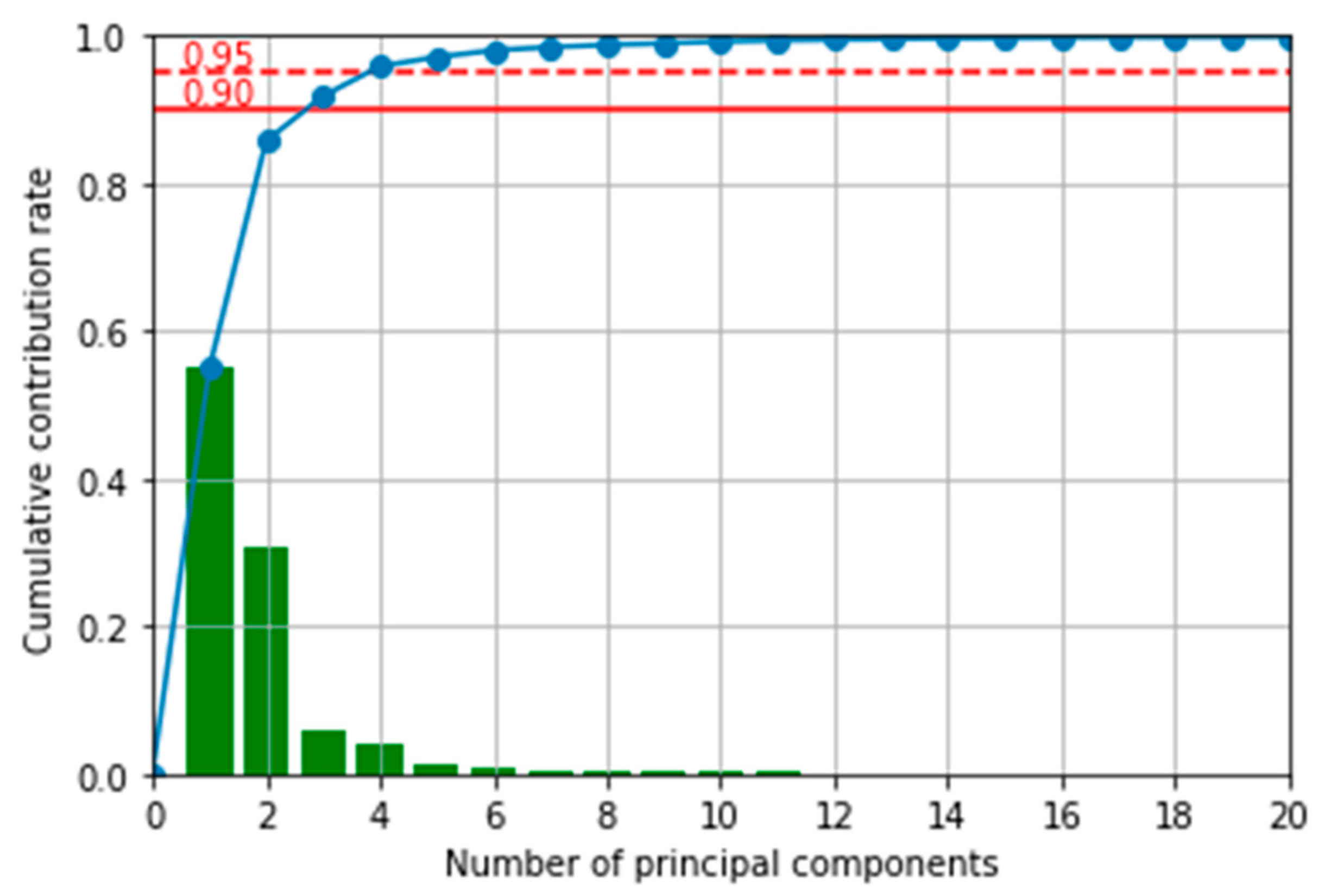
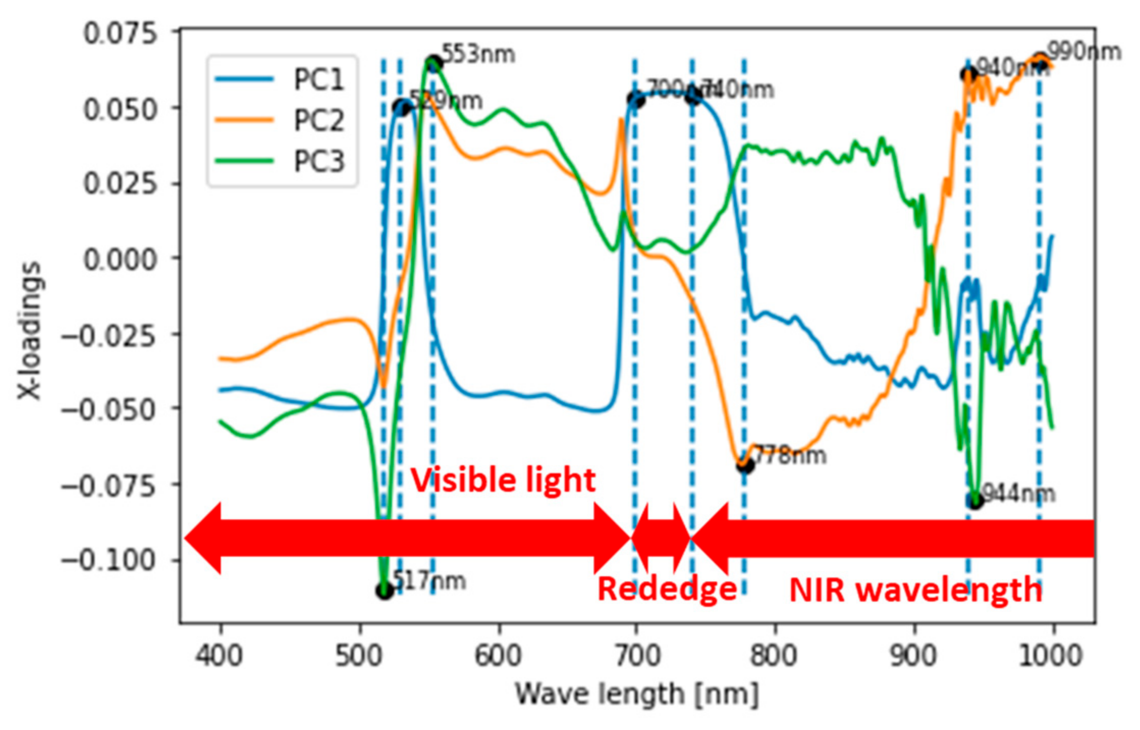
3.2.1. PCA Based Approach

Figure 7 shows the contribution rate and the cumulative contribution rate of components from PCA. From this figure, 90% of information is covered by three PCs, and 95% is covered by four PCs. Then, X-loadings were calculated of three principal components with the highest contribution rate.
Figure 8 shows the X-loadings value of the top three PCs, which covers 90% of the overall information. There are three peaks at around 530 nm, 700 nm, and over 900 nm, which are visible green, red edge, and NIR wavelengths, respectively. The list of bands known as absorption wavelengths of pasture components in the visible and near-infrared regions is shown in Table A1. Around 530 nm, where PC1, 2, and 3 have some peaks, there are crude protein wavelength bands at 535 nm and 545 nm. The wavelength band near the red edge 700–740 nm, where the peaks are seen in PC1 and 2, contains wavelength bands of major pasture components such as chlorophyll, neutral detergent fiber, and nitrogen and is commonly used in vegetation indices such as the normalized difference red edge index (NDRE) as an index for monitoring the vigor level of plants. The band of 900 nm and higher, which has many small peaks, mainly for PC2 and 3, has wavelength bands for proteins, lipids, and sugars, in addition to being highly absorbed by water.
Wavelength bands known to be sensitive to major grass constituents, as described above, were also detected as important in the X-loading analysis, and this result is considered reasonable since the grass samples collected throughout the two-year experiment should vary in terms of these compositions.
Table 4 shows the top 10 wavelengths with high loading values for PC1 and PC2, which explain 85% of all the information. They are divided into wavelengths around 530 nm and 700 nm, which are the range of red edge and visible green, respectively. In the vicinity of 736 nm and 734 nm, which showed high loadings, there is a wavelength band of 707 nm, which is known to be sensitive to nitrogen. As mentioned above, it is also a red-edge wavelength band widely used as a vegetation value. Around the neighborhood of 539 nm and 542 nm, which have high loads, there are wavelength bands of 535 nm and 545 nm that respond with crude protein. From the viewpoint of PCA data separation, components such as nitrogen, chlorophyll, and crude protein content vary greatly depending on the grass samples contributing to the distribution of the data. Therefore, the result is considered to be understandable.

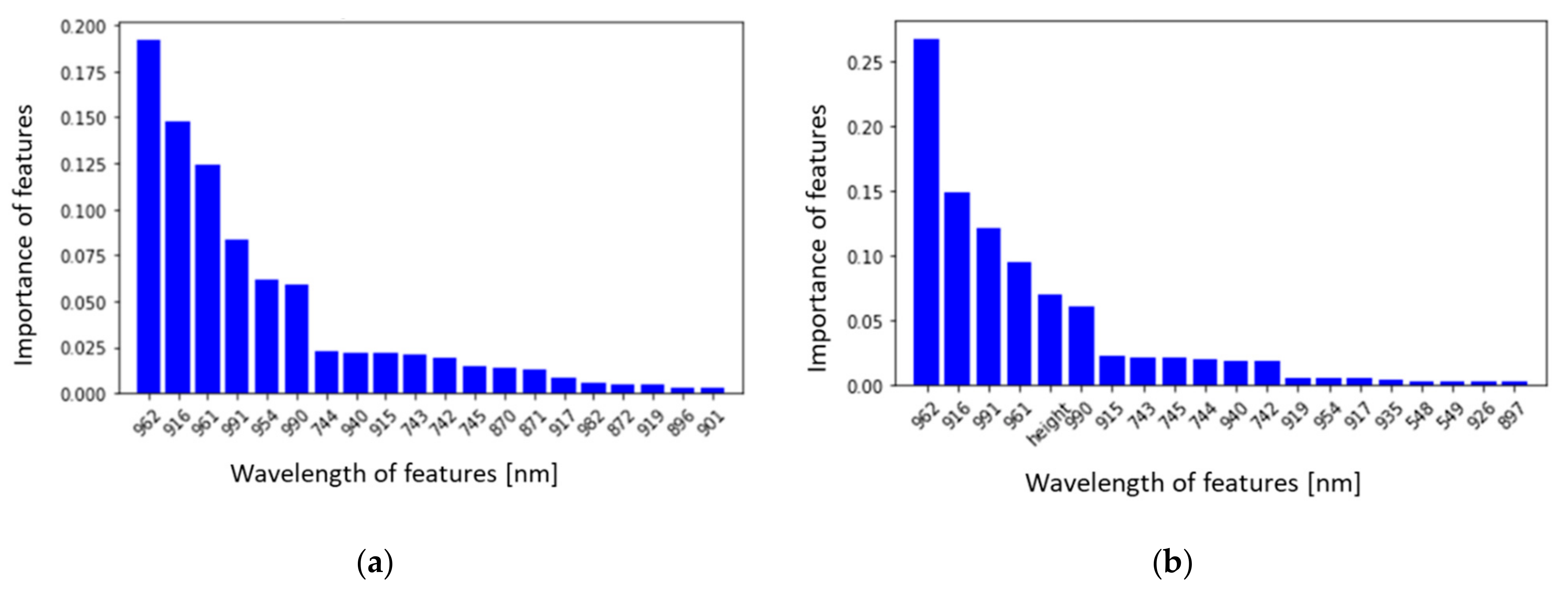
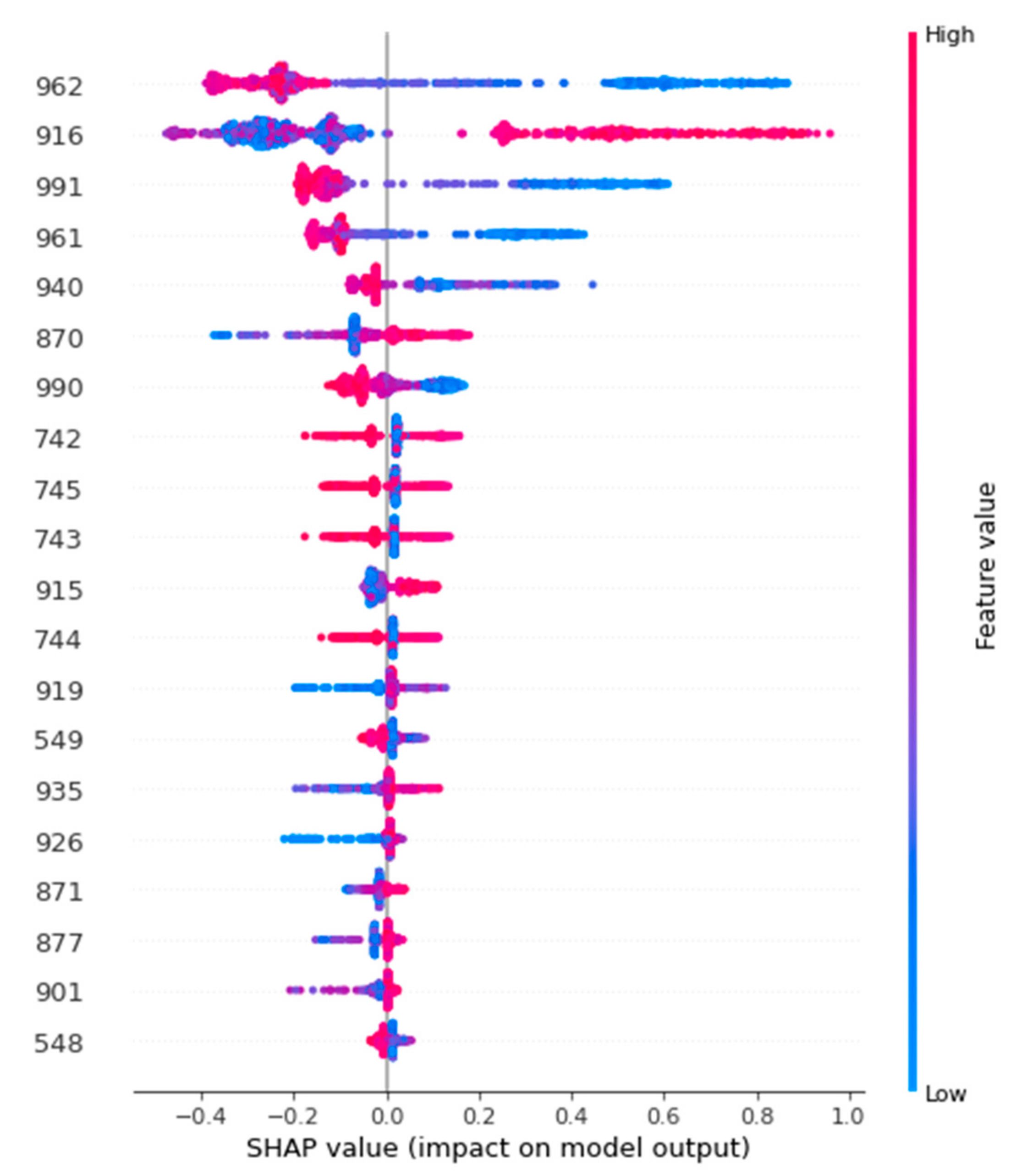
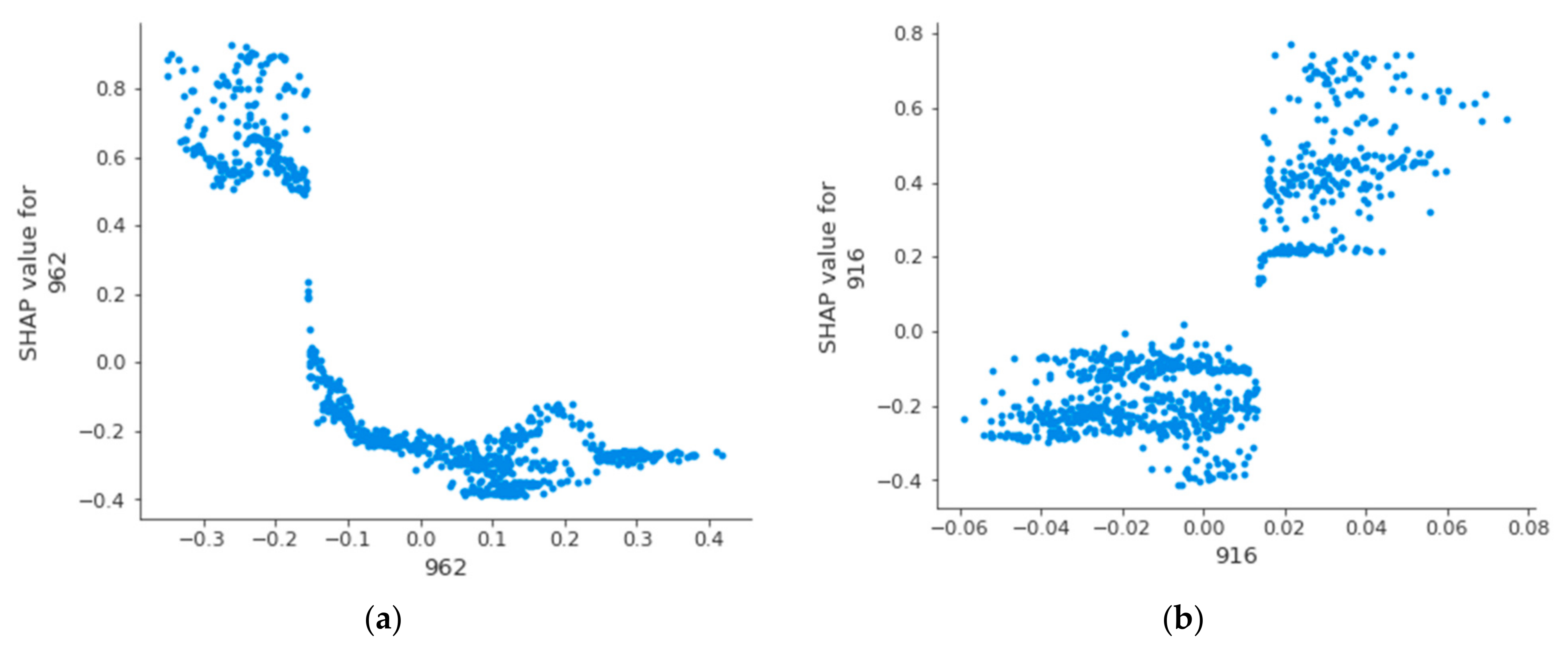
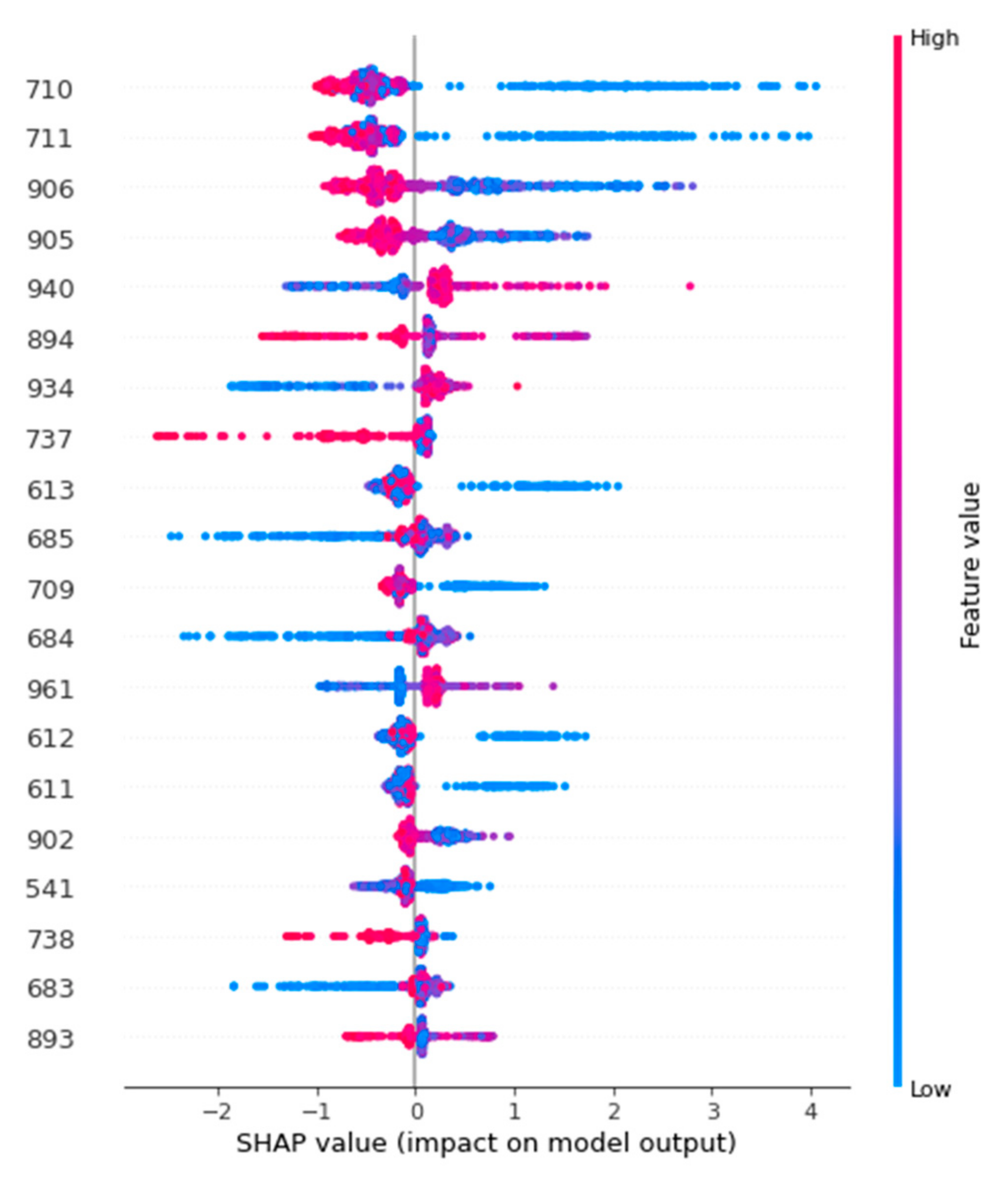
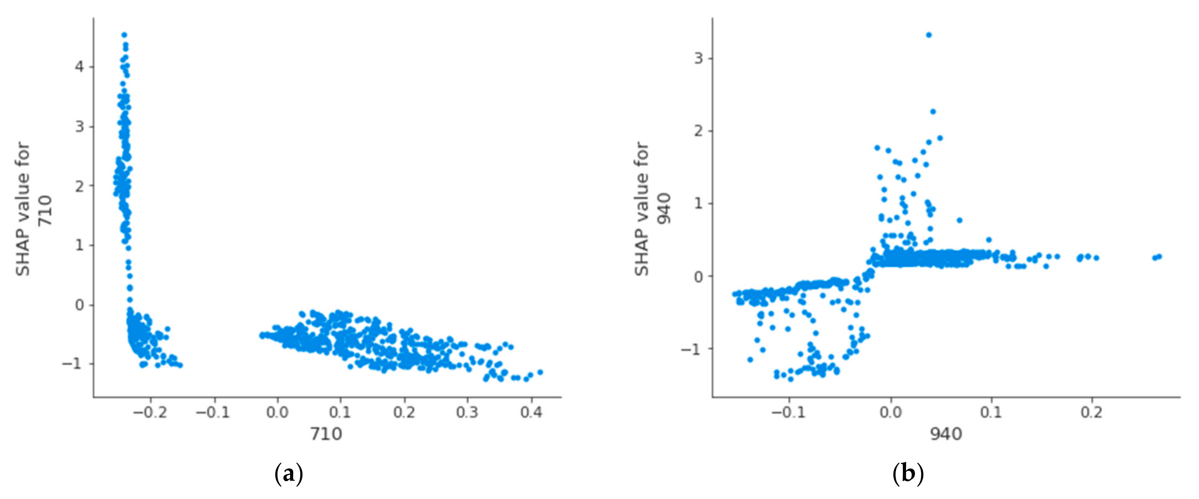
3.2.2. AI Model-Based Approach

By analyzing the structure of the random forest regressor model trained to estimate DMY and NC, the important wavelength for this purpose is revealed.
Figure 9 shows the importance of features to estimate DMY with/without height sensor data. For this purpose, the NIR wavelength range above 900 nm is judged as important both with and without a height sensor. Especially observed wavelength bands of 954 nm, 961 nm, 962 nm, 990 nm, and 991 nm are around 960 nm and 990 nm, which are reported to be related to starch and moisture. This is a reasonable result since starch is an important index which is related to grass growth, and water content obviously has a strong relation to DMY. Height sensor data also showed some amount of importance, and this is intuitively understandable.
Figure 10 represents the importance of features to estimate NC with/without height sensor data. In contrast to DMY estimating model, the red edge range strongly contributes to the estimation. NIR wavelengths and visible orange range around 600 nm also show high importance. This is a persuasive result since the wavelength bands determined to be important here are quite close to 705 nm and 721 nm, which are reported to be directly related to nitrogen, and wavelengths around 609 nm, 680 nm, and 705 nm, which are highly related to chlorophyll and neutral detergent fibers. When combined with height sensor data, this measurement data showed the greatest importance over the other wavelengths. The difference in importance between plant height and absorbance data is very large, but it is not an incorrect result simply because the amount of grass should be proportional to the amount of NC.
The top 20 SHAP values of the random forest regressor model, which was trained to estimate DMY (without height sensor data) are shown in Figure 11. In DMY estimation, NIR range is more relevant than the other wavelength range. The wavelengths chosen here are equivalent to the wavelengths chosen based on the feature importance of the random forest regressor. However, it also implies that a higher reflection value around 960 nm that is known to be relevant to water content, which means less water content, tends to result in less DMY. In contrast, a lower reflection value of 916 nm which is assigned to a higher amount of protein content, shows a negative relation to DMY. A higher reflection value of 916 nm, which means less protein content, can be both positive and negative in DM estimation, since red dots are observed for both positive and negative SHAP ranges.
Thus, unlike other methods such as random forest regressor, the biggest advantage of introducing SHAP is that it is possible to clearly indicate how “each feature value” of “each measurement data”, that is, the absorbance at each wavelength, affects the estimated target value.
Figure 12 shows the SHAP value transition over the feature value of random forest regressor to estimate DMY. Here, the features of 962 nm and 916 nm, which have high SHAP value contributions while having different trends, are chosen. From figure (a) 962 nm, the negative feature value tends to be higher in relation to the SHAP value, while the positive feature value tends to be a constant negative SHAP value around −0.3. In contrast, from Figure 12b, related to 916 nm, the positive feature value tends to be higher in relation to the SHAP value, while the negative feature value tends to lower the negative SHAP value. In addition, the range of the X-axis is −0.3 to −0.4 in the case of (a), while it is −0.06 to 0.08 in (b). This means that SHAP value varies considerably with little change in feature. Therefore, (b) is considered more sensitive to SHAP value.
In Figure 13, the top 20 SHAP values of the random forest regressor model for estimating NC (without height sensor data) are shown. The features identified as having high relevance by SHAP are also close to the wavelength selected based on the feature importance of the random forest regressor. From this figure, red edge wavelength is found to be relevant in addition to NIR range. Less reflection value around 710 nm and 906 nm that are known to be related to NC and protein content, respectively, in related research, which means a high amount of NC or protein content, also shows the high NC in this analysis. A higher reflection value around 940 nm which is known to be related to lipid content, which means less amount of lipid, shows the relation to higher NC.
Same as Figure 12, Figure 14 exhibits the SHAP value transition over the feature value of Random Forest Regressor to estimate NC. Here, the features of 710nm and 940nm, which have high SHAP value contributions while having different trends, are chosen. From the figure of (a) 710nm, the lower feature value than –0.2 shows a very high relation and sensitivity to the positive SHAP value, while a higher feature value than –0.2 tends to be a constant negative SHAP value around –0.1. In contrast, from the figure of (b) 940nm, positive/negative relation between feature value and SHAP value can be observed. Still, a constant SHAP value over any feature value around zero is also observed. This implies that there are cases where 940nm directly affects SHAP values, and cases where other features rather than 940nm are related to SHAP values.
As stated in the discussion for each result, most wavelengths revealed that strongly contribute to the estimation in this paper can be linked to well-known wavelengths in the related papers shown in Table A1. In addition, some negative relations, such as lipid content against NC are also revealed. More importantly, this SHAP analysis revealed: “how the feature value changes affected the output value of the regressor, which is represented as SHAP value.” This is clearly outstanding from previous research and may encourage the use of AI models that have been black boxes until now. It also provides more detailed analysis and insight into the field of multivariate analysis, such as spectroscopy, insisting on the possibility of finding previously missed relationships between measurement data and estimated values.

4. Conclusions

In this research, using data collected with a hyperspectral sensor from grassland under different fertilization schemes, a regression model was constructed to estimate the DMY and NC of grass. The wavelength bands useful for regression analysis were clarified by X-Loading analysis, feature quantity analysis, and SHAP analysis. From PCA based approach, the visible green wavelength (around 500 nm) and red edge wavelength (around 700 nm) are revealed to represent the overall variability. According to the analysis of the feature importance of the Random Forest Regressor, NIR wavelengths (around 960, 910, and 990 nm) are more sensitive to DMY estimation, while red edge (about 710 nm) and visible orange wavelengths (about 610 nm) are more related to NC estimation.
Moreover, by introducing SHAP analysis, not only the positive effect of features but also negative relations such as protein content (around 906 nm) against DMY estimation or lipid content (940 nm) against NC estimation can be revealed, which is capable of being introduced to other composition analysis as well in the future. This method offers new options for approaches such as spectroscopic analysis and sensor fusion using AI estimation models, which have high estimation accuracy but lack convincing results due to the difficulty of logically explaining their behavior. And this approach might give opportunities for detailed data analysis, which leads to finding previously missed data relationships.
In addition, estimation models of DMY and NC, in which plant height data was added to the input in addition to the hyperspectral sensor data, showed that the estimation accuracy was improved by 30% and 10%, respectively.
In future works, it would be interesting to compare the results which are measured in different environments, such as grasslands where legumes are the main species. If there are differences in the results, investigating the detailed reasons using the results of SHAP analysis will give new insights. In addition, by adding optimal data besides plant height, such as weather data and soil data, it will be possible to build a more accurate or robust measurement model.

Author Contributions

Conceptualization, H.N. and J.O.; methodology, software, validation and formal analysis, H.N.; investigation, H.N., K.J. and J.O.; resources and data curation, J.O., G.-J.N., F.S., F.H. and B.M.; writing—original draft preparation, H.N., J.O. and K.J.; writing—review and editing, H.N., J.O., K.J., I.H., C.K., P.v.d.V. and M.B.; visualization, H.N.; supervision, project administration and funding acquisition, C.K. All authors have read and agreed to the published version of the manuscript.

Funding

This research was founded by “Precision Agriculture 4.0” project and Public Private Project “DISAC (Data Intensive Smart Agrifood Chains)”. The APC was funded by Precision Agriculture 4.0. Keiji Jindo wishes to acknowledge financial support (3710473400).

Data Availability Statement

Not applicable.

Acknowledgments

We thank Peter van der Vlugt, Max Bouten, Leandro Santos and Masahiro Kawabata from Kubota Corporation for all the support and assistance with the discussion on data collection and technical comments in the frame of Public Private Project “DISAC (Data Intensive Smart Agrifood Chains)” and “Precision Agriculture 4.0”.

Conflicts of Interest

The authors declare no conflict of interest.

Appendix A

Appendix A.1. Outlier Removal

Outliers are the values obtained that have a large residual from their true value and are often included in real-world measurement data. Outliers have a negative impact on multivariate analysis or AI model performance and must be removed appropriately.
For this purpose, the isolation forest method [29] which classifies outliers based on the distance of decision tree structure was applied. Since isolation forest is one of the unsupervised methods, it does not require the definition of ‘correct data’ by user parameters. In isolation forest, an anomaly score s(x, n) for each sample x was defined as the following Equation (A1):
s x , n = 2 E h x c n
where E(h(x)) is the average value of h(x) on the set of isolation trees, h(x) is the height of sample x in each isolation tree, and c(n) is the average path length (depth) for binary search. In this way, s(x, n) is regularized between 0 and 1. Since the number of anomaly data is small and separated at early stage (or shallow part of the tree), the sample x which has s(x, n) close to 1 is anomaly data. In contrast, the sample x which has smaller s(x, n) is classified as normal data. ‘Contamination’ is a parameter that defines how much anomaly data is included in the dataset. Here it is set to 0.05. Depending on the magnitude of s(x, n), data with the ratio determined by the parameter is removed as anomaly data. Figure A1. shows the remaining spectrum and separated spectrum after applying outlier removal.
Figure A1. Normal and outlier spectrum separated by isolation forest: (a) Normal data separated from all the measurement hyper spectrum data by isolation forest (n = 4154); (b) Remaining outliers separated by isolation forest (n = 904). X-axis represents wavelength of feature (Unit: nm) while Y-axis represents reflection value (Unit: Reflection Unit). The color of lines represents each reflectance value of grass samples.
Remotesensing 15 00419 g0a1

Appendix A.2. Correction of Variation

Near-infrared spectroscopy reflectance data from non-uniform samples such as grass contain noise due to variations in optical path length and light scattering. To reduce and compensate for these effects, standard normal variate (SNV) [30] or multiplicative scatter correction (MSC) are generally used [31]. In this experiment, since the reference spectrum which is required in MSC is unavailable, SNV was applied. After applying SNV, standard deviation of each wavelength is set to be one. Corrected spectrum by SNV is shown in Figure A2. In this research, since the amount of ambient light varied greatly for each measurement because of the outdoor reflection measurement from a distance of about 1 m, it is considered that the correction of variation worked well.
Figure A2. Spectrum corrected by standard normal variate (SNV). X-axis represents wavelength of feature (Unit: nm) while Y-axis represents standardized reflection value. The color of lines represents each reflectance value of grass samples.
Remotesensing 15 00419 g0a2

Appendix A.3. Centering

In order to obtain better results in multivariate analysis, the mean and standard deviation of the values for each variable need to be standardized to be treated equally. Since standard deviation is already corrected throughout applying SNV, centering is applied here to correct the mean value. AI models such as random forest regressor focus on changes in features between data, so there is no adverse effect from centering. Since PCA includes centering in its algorithm, it is not necessary to apply centering, but there is no problem if it is applied. Centering the spectrum x is calculated as following Equation (A2):
C e n t e r x = x E x
where, E(x) is the average value of x. Corrected spectrum by centering is shown as Figure A3. By applying this, the signal strength at each wavelength is standardized, and the difference in the signal of the wavelength where the change in reflection is large is emphasized.
Figure A3. Spectrum corrected by centering. X-axis represents wavelength of feature (Unit: nm) while Y-axis represents standardized and centered reflection value. The color of lines represents each reflectance value of grass samples.
Remotesensing 15 00419 g0a3

Appendix B

Table A1 shows the wavelength which has a strong contribution to estimation through experimental results, and the well-known wavelength which has similar range to the experimental results of this paper.
Table A1. Contributed wavelength to estimation model, well-known wavelength and their chemical/biochemical characteristics.
Wavelength (nm)Electron Transition/Bond Vibration/Red EdgeBiochemical ComponentExperiment in This ResearchReferences
430Electron transitionChlorophyll a-[32]
460Electron transitionChlorophyll b-[32]
523Electron transition-3.2.1. PC1/2-
530Electron transition-3.2.1 X-loadings-
532Electron transition-3.2.1 PC1/2-
535Electron transitionCrude protein-[13]
539Electron transition-3.2.1 PC1/2-
542Electron transition-3.2.1 PC1/2-
545Electron transitionCrude protein-[13]
609Electron transitionChlorophyll --
612Electron transition-3.2.2. NC estimation-
680Red edgeChlorophyll
Neutral detergent fiber
-[32,33]
698Red edge-3.2.1 PC1/2-
699Red edge-3.2.1 PC1/2-
705Red edgeNeutral detergent fiber-[32]
707Red edgeNitrogen-[12]
710Red edge-3.2.2 NC estimation
711Red edge-3.2.2 NC estimation
721Red edgeNitrogen-[12]
734Red edge-3.2.1 PC1/2-
736Red edge-3.2.1 PC1/2-
895--3.2.2 NC estimation
910C-H stretch, 3rd overtoneProtein-[32]
912C-H stretch, 3rd overtone-3.2.2 DMY estimation
930C-H stretch, 3rd overtoneLipid-[32]
940C-H stretch, 3rd overtone-3.2.2 NC estimation
X-loadings (PC1)
960O-H bend, 1st overtone-3.2.2 DMY estimation
970O-H bend, 1st overtoneWater, starch-[32]
990O-H stretch, 2nd overtoneStarch-[32]
991O-H stretch, 2nd overtone-3.2.2 DMY estimation-

References

  1. Eurostat. Share of Main Land Types in Utilised Agricultural Area (UAA) by NUTS 2 Regions; Eurostat: Luxembourg, 2020. [Google Scholar]
  2. Schils, R.L.M.; Van den Berg, W.; Van der Schoot, J.R.; Groten, J.A.M.; Rijk, B.; Van de Ven, G.W.J.; Van Middelkoop, J.C.; Holshof, G.; Van Ittersum, M.K. Disentangling genetic and non-genetic components of yield trends of Dutch forage crops in the Netherlands. Field Crops Res. 2020, 249, 107755. [Google Scholar] [CrossRef]
  3. Schils, R.L.; Bufe, C.; Rhymer, C.M.; Francksen, R.M.; Klaus, V.H.; Abdalla, M.; Milazzo, F.; Lellei-Kovács, E.; ten Berge, H.; Bertora, C.; et al. Permanent grasslands in Europe: Land use change and intensification decrease their multifunctionality. Agric. Ecosyst. Environ. 2022, 330, 107891. [Google Scholar] [CrossRef]
  4. Smit, H.; Metzger, M.; Ewert, F. Spatial distribution of grassland productivity and land use in Europe. Agric. Syst. 2008, 98, 208–219. [Google Scholar] [CrossRef]
  5. Robertson, G.P.; Vitousek, P.M. Nitrogen in agriculture: Balancing the cost of an essential resource. Annu. Rev. Environ. Resour. 2009, 34, 97–125. [Google Scholar] [CrossRef] [Green Version]
  6. Oenema, J.; van Ittersum, M.; van Keulen, H. Improving nitrogen management on grassland on commercial pilot dairy farms in the Netherlands. Agric. Ecosyst. Environ. 2012, 162, 116–126. [Google Scholar] [CrossRef]
  7. Zhao, Y.R.; Yu, K.Q.; Li, X.; He, Y. Detection of Fungus Infection on Petals of Rapeseed (Brassica napus L.) Using NIR Hyperspectral Imaging. Sci. Rep. 2016, 6, 38878. [Google Scholar] [CrossRef]
  8. Thenkabail, P.S.; Smith, R.B.; De Pauw, E. Evaluation of narrowband and broadband vegetation indices for determining optimal hyperspectral wavebands for agricultural crop characterization. Photogramm. Eng. Remote Sens. 2002, 68, 607–621. [Google Scholar]
  9. Yi, Q.-X.; Huang, J.-F.; Wang, F.-M.; Wang, X.-Z.; Liu, Z.-Y. Monitoring rice nitrogen status using hyperspectral reflectance and artificial neural network. Environ. Sci. Technol. 2007, 41, 6770–6775. [Google Scholar] [CrossRef] [PubMed]
  10. Thenkabail, P.S.; Enclona, E.A.; Ashton, M.S.; Van Der Meer, B. Accuracy assessments of hyperspectral waveband performance for vegetation analysis applications. Remote Sens. Environ. 2004, 91, 354–376. [Google Scholar] [CrossRef]
  11. Chan, J.C.W.; Paelinckx, D. Evaluation of Random Forest and Adaboost tree-based ensemble classification and spectral band selection for ecotope mapping using airborne hyperspectral imagery. Remote Sens. Environ. 2008, 112, 2999–3011. [Google Scholar] [CrossRef]
  12. Kawamura, K.; Watanabe, N.; Sakanoue, S.; Lee, H.-J.; Inoue, Y. Waveband selection using a phased regression with a bootstrap procedure for estimating legume content in a mixed sown pasture. Jpn. Soc. Grassl. Sci. Grassl. Sci. 2011, 57, 81–93. [Google Scholar] [CrossRef]
  13. Alckmin, G.; Lucieer, A.; Roerink, G.; Rawnsley, R.; Hoving, I.; Kooistra, L. Retrieval of Crude Protein in Perennial Ryegrass Using Spectral Data at the Canopy Level. Remote Sens. 2020, 12, 2958. [Google Scholar] [CrossRef]
  14. Liaw, A.; Wiener, M. Classification and Regression by randomForest. R News 2002, 2, 18–22. [Google Scholar]
  15. Kawamura, K.; Watanabe, N.; Sakanoue, S.; Inoue, Y.; Odagawa, S.; Lee, H.-J. Testing genetic algorithm as a tool to select relevant wavebands from field hyperspectral data for estimating pasture mass and quality in a mixed sown pasture using partial least squares regression. Grassl. Sci. 2010, 56, 205–216. [Google Scholar] [CrossRef]
  16. Lobos, I.; Moscoso, C.J.; Pavez, P. Calibration models for the nutritional quality of fresh pastures by nearinfrared reflectance spectroscopy. Cienc. Investig. Agrar. 2019, 46, 234–242. [Google Scholar] [CrossRef]
  17. Parrini, S.; Acciaioli, A.; Franci, O.; Pugliese, C.; Bozzi, R. Near Infrared Spectroscopy technology for prediction of chemical composition of natural fresh pastures. J. Appl. Anim. Res. 2019, 47, 514–520. [Google Scholar] [CrossRef] [Green Version]
  18. Alomar, D.; Fuchslocher, R.; Cuevas, J.; Mardones, R.; Cuevas, E. Prediction of the composition of fresh pastures by near infrared reflectance or interactance-reflectance spectroscopy. Chil. J. Agric. Res. 2009, 69, 198–206. [Google Scholar] [CrossRef] [Green Version]
  19. Park, R.S.; Agnew, R.E.; Gordon, F.J.; Steen, R.W.J. The use of near infrared reflectance spectroscopy (NIRS) on undried samples of grass silage to predict chemical composition and digestibility parameters. Anim. Feed. Sci. Technol. 1998, 72, 155–167. [Google Scholar] [CrossRef]
  20. Sage, A.J. Random Forest Robustness, Variable Importance, and Tree Aggregation. Ph.D. Thesis, Iowa State University, Ames, IA, USA, 2018. [Google Scholar]
  21. Khanal, K.; Bhusal, S.; Karkee, M.; Zhang, Q. Distinguishing One Year and Two Year Old Canes of Red Raspberry Plant using Spectral Reflectance. IFAC-PapersOnLine 2018, 51, 39–44. [Google Scholar] [CrossRef]
  22. Lundberg, S.M.; Lee, S.I. A Unified Approach to Interpreting Model Predictions. In Proceedings of the 31st Conference on Neural Information Processing Systems (NIPS 2017), Long Beach, CA, USA, 4–9 December 2017. [Google Scholar]
  23. Burns, G.A.; Gilliland, T.J.; Grogan, D.; Watson, S.; O’Kiely, P. Assessment of herbage yield and quality traits of perennial ryegrasses from a national variety evaluation scheme. J. Agric. Sci. 2013, 151, 331–346. [Google Scholar] [CrossRef]
  24. Jafari, A.; Connolly, V.; Frolich, A.; Walsh, E.J. A Note on Estimation of Quality Parameters in Perennial Ryegrass by near Infrared. Ir. J. Agric. Food Res. 2003, 42, 293–299. [Google Scholar]
  25. Murphy, D.J.; O’Brien, B.; O’Donovan, M.; Condon, T.; Murphy, M.D. A near infrared spectroscopy calibration for the prediction of fresh grass quality on Irish pastures. Inf. Process. Agric. 2022, 9, 243–253. [Google Scholar] [CrossRef]
  26. Klaus, V.H.; Kleinebecker, T.; Boch, S.; Müller, J.; Socher, S.A.; Prati, D.; Fischer, M.; Hölzel, N. NIRS meets Ellenberg’s indicator values: Prediction of moisture and nitrogen values of agricultural grassland vegetation by means of near-infrared spectral characteristics. Ecol. Indic. 2012, 14, 82–86. [Google Scholar] [CrossRef]
  27. Bonnal, L.; Julien, L.; Delalande, M.; Bastianelli, D. How can a dry forage database be used to predict fresh grass composition by NIR spectroscopy? Data transfer vs spectra transfer. In Proceedings of the International Conference on Near Infrared Spectroscopy (NIR 2013), La Grande-Motte, France, 2–7 June 2013; Maurel, V.B., Williams, P., Downey, G., Kaboré, R., Eds.; IRSTEA—France Institut National de Recherche en Sciences et Technologies pour L’environnement et L’agriculture: Montpellier, France, 2013; Volume 16, pp. 685–693. [Google Scholar]
  28. McClure, W.F.; Crowell, B.; Stanfield, D.L.; Mohapatra, S.; Morimoto, S.; Batten, G. Near infrared technology for precision environmental measurements: Part 1. Determination of nitrogen in green- and dry-grass tissue. J. Infrared Spectrosc. 2002, 10, 177–185. [Google Scholar] [CrossRef]
  29. Liu, F.T.; Ting, K.M.; Zhou, Z.H. Isolation Forest. In Proceedings of the 2008 Eighth IEEE International Conference on Data Mining, Pisa, Italy, 15–19 December 2008. [Google Scholar]
  30. Barnes, R.J.; Dhanoa, M.S.; Lister, S.J. Standard Normal Variate Transformation and De-Trending of Near-Infrared Diffuse Reflectance Spectra. Appl. Spectrosc. 1989, 43, 772–777. [Google Scholar] [CrossRef]
  31. Geladi, P.; MacDougall, D.; Martens, H. Linearization and Scatter-Correction for Near-Infrared Reflectance Spectra of Meat. Appl. Spectrosc. 1985, 39, 491–500. [Google Scholar] [CrossRef]
  32. Curran, P.J. Remote sensing of foliar chemistry. Remote Sens. 1989, 30, 271–278. [Google Scholar] [CrossRef]
  33. Post, C.J.; Degloria, S.D.; Cherney, J.H.; Mikhailova, E.A. Spectral Measurements of Alfalfa/Grass Fields Related to Forage Properties and Species Composition. J. Plant Nutr. 2007, 30, 1779–1789. [Google Scholar] [CrossRef]
Figure 1. Design of experimental fields: (a) Wageningen test site (clay soil); (b) De Marke test site (sandy soil).
Remotesensing 15 00419 g001
Figure 2. Sensors used to measure grass in the field experiment.
Remotesensing 15 00419 g002
Figure 3. Histograms of measured data during harvest in 2019 and 2020: (a) DMY in 2019 and 2020; (b) NC in 2019 and 2020; (c) Grass height in 2019 and 2020. The width of the graph represents the number of samples, while Y-axis corresponds to the measured variables. The measurement of DMY and NC were conducted by using the absolute dry method and the “digestion H2SO4-H2O2-Se; SFA-Nt/Pt” method, respectively. In addition, grass height was measured by ultrasonic sensor.
Remotesensing 15 00419 g003
Figure 4. Flowchart of data pre-process of measured data.
Remotesensing 15 00419 g004
Figure 5. Structure of random forest regressor.
Remotesensing 15 00419 g005
Figure 6. Plots of ground truth and predicted values. X-axis represents the ground truth data of the test dataset. In contrast, the Y-axis represents the predicted values by random forest regressor model using input features of the test data set. (a) DMY using hyperspectral data as input; (b) DMY using hyperspectral data and height data; (c) NC using hyperspectral data as input; (d) NC using hyperspectral data and height data.
Remotesensing 15 00419 g006
Figure 7. The cumulative contribution rate of components from PCA. The X-axis represents PCs sorted in ascending order of contribution rate, while the bar and line charts of the Y-axis represent contribution rates and cumulative contribution rates, respectively.
Remotesensing 15 00419 g007
Figure 8. X-loadings analysis of Principal Component Analysis (PCA). X-axis represents wavelength of feature (Unit: nm) while Y-axis represents X-loading values of Principal Components.
Remotesensing 15 00419 g008
Figure 9. Importance of features of random forest regressor. (a) Trained to estimate DMY from hyper spectrum; (b) Trained to estimate DMY from the hyper spectrum with grass height. X-axis represents the wavelength of the feature (Unit: nm) or grass height (indicated as height), while the Y-axis represents the importance of features.
Remotesensing 15 00419 g009
Figure 10. Importance of features of random forest regressor. (a) Trained to estimate NC from hyper spectrum; (b) Trained to estimate NC from the hyper spectrum with grass height. X-axis represents the wavelength of feature (Unit: nm) or grass height (indicated as height) while Y-axis represents the importance of features.
Remotesensing 15 00419 g010
Figure 11. Shapley additive explanations (SHAP) value analysis for DMY. X-axis represents SHAP value while Y-axis represents wavelength of feature (Unit: nm). Color represents the reflection value of each feature.
Remotesensing 15 00419 g011
Figure 12. Shapley additive explanations (SHAP) value transition over feature value of random forest regressor to estimate DM content. (a) SHAP value for the feature of 962 nm; (b) SHAP value for the feature of 916 nm. X-axis represents feature value while Y-axis represents SHAP value.
Remotesensing 15 00419 g012
Figure 13. Shapley additive explanations (SHAP) value analysis for NC. X-axis represents SHAP value while Y-axis represents the wavelength of the feature (Unit: nm).
Remotesensing 15 00419 g013
Figure 14. Shapley additive explanations (SHAP) value transition over feature value of random forest regressor to estimate NC. (a) SHAP value for the feature of 710 nm; (b) SHAP value for the feature of 940 nm. X-axis represents feature value while Y-axis represents SHAP value.
Remotesensing 15 00419 g014
Table 1. Measured Parameters of Grass.
Measured ParameterTechnological Device or Method for Data AcquisitionDuring Harvest Lab Analysis
Plant height (cm)Pasture Readerx
Fresh Grass Weight (t/ha)Weight scalex
Hyper Spectrum reflectanceTec5 HandySpec Field equipmentx
DMY (t/ha)Absolutely dry method x
NC (g N/kg DM)Digestion H2SO4-H2O2-Se; SFA-Nt/Pt x
Table 2. Performance of estimation by random forest regressor using statistical parameters of r- squared (r2), root-mean-square deviation (RMSE) and mean absolute error (MAE).
DMYDMY
(with Height)
NCNC
(with Height)
r20.940.970.880.90
RMSE0.350.172.592.35
MAE0.230.251.881.68
Table 3. Performance of calibrations for DMY, NC or crude protein (CP) in related research.
StudyCountryAnalyteParametersSampler2 RMSE
DMYCP, NCDMYCP, NC
[13]Austria,
Netherlands
Fresh grassCP231-0.81-85.5 kg CP/ha
[15]JapanFresh grassCP100-0.85-6.46 g/DM kg
[25]IrelandFresh grassDMY, CP490.860.849.46 g/kg20.38 g/DM kg
[26]GermanyDried, milled grassMoisture, CP18120.910.840.450.47
[16]ChileFresh grassDMY, CP9150.930.8411.3 g/kg22.2 g/DM kg
[17]ItalyFresh grassDMY, CP1000.870.882.75 g/kg2.14 g/DM kg
[27]FranceFresh grassCP103-0.93-1.55 g/DM kg
[18]ChileFresh grassDMY, CP1070.990.916.55 g/kg18.4 g/DM kg
[28]USAFresh grassNC31-0.88-6 g/DM kg
[19]IrelandFresh grass silageDM, NC1360.850.78-4.8 g/DM kg
[23]IrelandDried, milled grassCP2076-0.98--
[24]IrelandDried, milled grassCP153-0.96--
Table 4. Top 10 wavelength which have high loadings for PC1 and PC2.
Wavelength [nm]Loading
7360.485
5390.396
7340.384
5420.371
6990.262
5320.217
5230.214
6980.213
5310.197
5340.187
Disclaimer/Publisher’s Note: The statements, opinions and data contained in all publications are solely those of the individual author(s) and contributor(s) and not of MDPI and/or the editor(s). MDPI and/or the editor(s) disclaim responsibility for any injury to people or property resulting from any ideas, methods, instructions or products referred to in the content.

