Article

Gap-Filling Sentinel-1 Offshore Wind Speed Image Time Series Using Multiple-Point Geostatistical Simulation and Reanalysis Data

by
Stylianos Hadjipetrou
1,*,
Gregoire Mariethoz
2 and
Phaedon Kyriakidis
1
1
Department of Civil Engineering and Geomatics, Cyprus University of Technology, Limassol 3036, Cyprus
2
Institute of Earth Surface Dynamics, University of Lausanne, 1015 Lausanne, Switzerland
*
Author to whom correspondence should be addressed.
Remote Sens. 2023, 15(2), 409; https://doi.org/10.3390/rs15020409
Submission received: 28 November 2022 / Revised: 31 December 2022 / Accepted: 6 January 2023 / Published: 9 January 2023

Abstract

:
Offshore wind is expected to play a key role in future energy systems. Wind energy resource studies often call for long-term and spatially consistent datasets to assess the wind potential. Despite the vast amount of available data sources, no current means can provide relevant sub-daily information at a fine spatial scale (~1 km). Synthetic aperture radar (SAR) delivers wind field estimates over the ocean at fine spatial resolution but suffers from partial coverage and irregular revisit times. Physical model outputs, which are the basis of reanalysis products, can be queried at any time step but lack fine-scale spatial variability. To combine the advantages of both, we use the framework of multiple-point geostatistics to realistically reconstruct wind speed patterns at time instances for which satellite information is absent. Synthetic fine-resolution wind speed images are generated conditioned to coregistered regional reanalysis information at a coarser scale. Available simultaneous data sources are used as training data to generate the synthetic image time series. The latter are then evaluated via cross validation and statistical comparison against reference satellite data. Multiple realizations are also generated to assess the uncertainty associated with the simulation outputs. Results show that the proposed methodology can realistically reproduce fine-scale spatiotemporal variability while honoring the wind speed patterns at the coarse scale and thus filling the satellite information gaps in space and time.

1. Introduction

Renewable energy sources (RES) appear as a solution for decarbonizing the energy sector. Offshore wind has been recognized as a key contributor to a more sustainable green energy production worldwide. A substantial increase in annual installed capacity in the last decade demonstrates the promising potential for such energy systems [1,2]. A critical step prior to exploiting wind energy is the assessment of the wind resource potential at regional and local scales using long-term datasets. While originally developed for weather forecasting, numerical weather prediction (NWP) mesoscale models are routinely used to obtain the required wind speed distributions [3,4]. When the model outputs are combined with observations via a data assimilation process to account for biases, the resulting gridded datasets are referred to as reanalysis data [5]. Despite their temporally continuous and spatially exhaustive coverage, computational and other constraints limit the spatial resolution of reanalysis data (ranging between 5 and 50 km), thus hindering their utility in the assessment of wind resources at the local scale, for which finely resolved data products are needed [5,6,7]. Therefore, the inherent spatiotemporal variability of wind speed cannot be derived from such coarse-scale models. Furthermore, NWP-derived wind profile uncertainty cannot be directly quantified and propagated to subsequent wind energy analyses [8].
Given the limitations of reanalysis-based estimates, alternative data sources have been used to supplement the information provided by mesoscale models. Because in situ measurements over the ocean are rather sparse, satellite-based remote sensing has been widely exploited to acquire detailed knowledge of offshore wind speed spatiotemporal variations. Active microwave sensors, such as synthetic aperture radar (SAR) and Scatterometers (SCATs) have been providing images pertaining to offshore wind for more than 20 years, and future satellite missions are already being planned or considered [9]. This cost-efficient information is vital for a plethora of energy-related applications ranging from pinpointing ideal wind farm siting locations [10,11,12] to identifying wake effects downstream of offshore wind farms [13,14]. While both SAR and SCAT sensors retrieve wind speed information in a similar way via the inversion of an empirical geophysical model function (GMF) relating backscattered normalized radar cross section (NRCS) to incidence angle and near-surface wind speed and direction, they mainly differ in terms of spatial resolution [15]. SAR has prevailed over SCAT for wind speed retrievals due to its relatively fine spatial resolution and consequent ability to detect small-scale offshore wind variations, in particular close to the coast [16,17]. SAR sensors, such as those mounted on ERS-1 and 2, ENVISAT, RADARSAT-1 and 2, TerraSAR-X and, most recently, on Sentinel-1A and 1B satellites, have been operating at different wavelength bands to provide the means for retrieving wind speed over the ocean surface. The exploitation of Sentinel-1 SAR data, in particular, has been attracting increasing interest in an attempt to obtain an accurate characterization of offshore wind regimes. Relevant examples include the recent work of [18] focused on the offshore area around Cyprus, as well as the case studies of [19] and [20] assessing wind resource potential using Sentinel-1 SAR estimates northwest and northeast of Sardinia and offshore Ireland, respectively. The main drawback of utilizing Sentinel-1 SAR data for wind resource potential assessment, as concluded in all the studies mentioned above, is the relatively short data time series (2014-present) and the limited number of estimates derived from the sensors, as the satellite orbit leads to gaps between consecutive passes [21]. In the absence of such information, spatiotemporal prediction or simulation methods must be employed to form a complete and consistent image time series, thus filling the missing satellite information (gaps) necessary for a thorough wind resource assessment while preserving the local wind features. To the best of our knowledge, few studies have attempted to address this problem by assimilating coarse-scale remote sensing or reanalysis data via a simulation approach [22,23] and even fewer within a geostatistical context. Moreover, existing studies have focused on reconstructing missing values due to, for example, cloud contamination (in the case of optical sensing) or systematic errors in the relevant satellite images rather than simulating large continuous patterns or even entire images in the time series. Although this literature gap was first identified by [24], referred to as “weakly constrained gap-filling problems”, limited progress has been made since.
The applicability of multiple-point (geo)statistics (MPS) in the reconstruction of spatial and/or temporal patterns across multiple scales has been previously demonstrated in a variety of fields. [24] pioneered the use of MPS simulation to fill artificially imposed gaps of weather research and forecasting (WRF) simulation outputs pertaining to latent heat flux, surface temperature and soil moisture. [25] followed a similar approach using a 20-year time series of both coarse- and fine-spatial-resolution WRF outputs as training data to simulate fine-scale data for future dates for which only coarse-scale outputs were available. The work was later extended in an attempt to downscale temperature, along with a highly non-stationary variable (i.e., precipitation), considering their interdependencies [26]. Although the above studies proved that MPS can simultaneously account for complex structural and textural properties, as well as non-linear dependencies among multiple interrelated variables, they involve coarse-resolution model-derived data that do not exhibit strong temporal variability. Moreover, in the former case, relatively small gaps were filled, whereas in the latter two cases, a fully informed and sufficiently long time series is assumed to be available as training data. [27] study based on Landsat 7 imagery was the only attempt involving satellite data in the MPS gap-filling simulation process. In this case, however, single images were considered rather than image time series, with the study being focused on highlighting the method’s ability to reconstruct spatial heterogeneity across different regions. Most recently, [28] investigated the efficiency of MPS to simulate rainfall fields using radar images as training data. The main novelty of this work is related to the classification of weather patterns using a set of climate indicators and their subsequent use to create conditional training image sets (CTIS). Daily rainfall was then simulated conditionally on a selected CTIS with a similar weather state.
In a similar way, we formed a multivariate CTIS by selecting pairs of uncertainties in ensembles of regional reanalyses (UERRA) and Sentinel-1 images to simulate the missing Sentinel-1 information. However, the underlying physical laws of wind fields are not described using a set of climate data but considered to be expressed by the physics-based UERRA model outputs. Therefore, no multiple-point statistics are required to generate the TIs, which are directly selected by the historical record using a statistical metric instead. The selected CTIS for each gap datetime is then used to simulate the missing wind fields at the fine scale.
Accordingly, the aim of this work was to further advance the use of MPS for spatiotemporal gap filling by simulating fine-scale offshore wind speed patterns around Cyprus via the combined use of fine-scale satellite-derived wind speed estimates, thus retaining the spatial variability of wind speed at the local scale, with physics-informed reanalysis model data, from which coarse-scale wind speed pattern norms are inherited. The contribution of this work is summarized in the following points:
  • A novel TI selection method is presented to form the CTIS used to simulate the missing patterns at each time step. This method is based on the dependence between the coregistered coarse- and fine-scale information included in the training images. Once the CTIS is formed, fine-scale patterns are simulated and locally conditioned to the coarse-scale data.
  • An MPS algorithm recently developed by [29], namely quick sampling (QS), is exploited for the first time in a spatiotemporal gap-filling application. The precise aim of this study is to take advantage of the robustness and computational efficiency of the algorithm to investigate its potential to provide realistic reconstructions of spatially complex patterns of continuous fields.
  • A first real-world case study of image time-series expansion is provided in an offshore wind speed context by generating wind fields of realistic spatial and temporal variability while preserving the complex multivariate wind relationships. Considering the complex variability and dynamic nature of wind speed both in space and time, this endeavor is rather challenging and often fails to reproduce the inherent variability at the fine scale, especially when long-term training datasets are not available.
The remainder of this paper is structured as follows. The data sources and the study area considered in this work are described in the subsequent section. The adopted methodological framework and the validation tools employed in this study are presented in Section 3. Section 4 presents and analyzes the simulation outputs and the evaluation results. Finally, Section 5 and Section 6 are dedicated to discussion, as well as conclusions and future research outlooks.

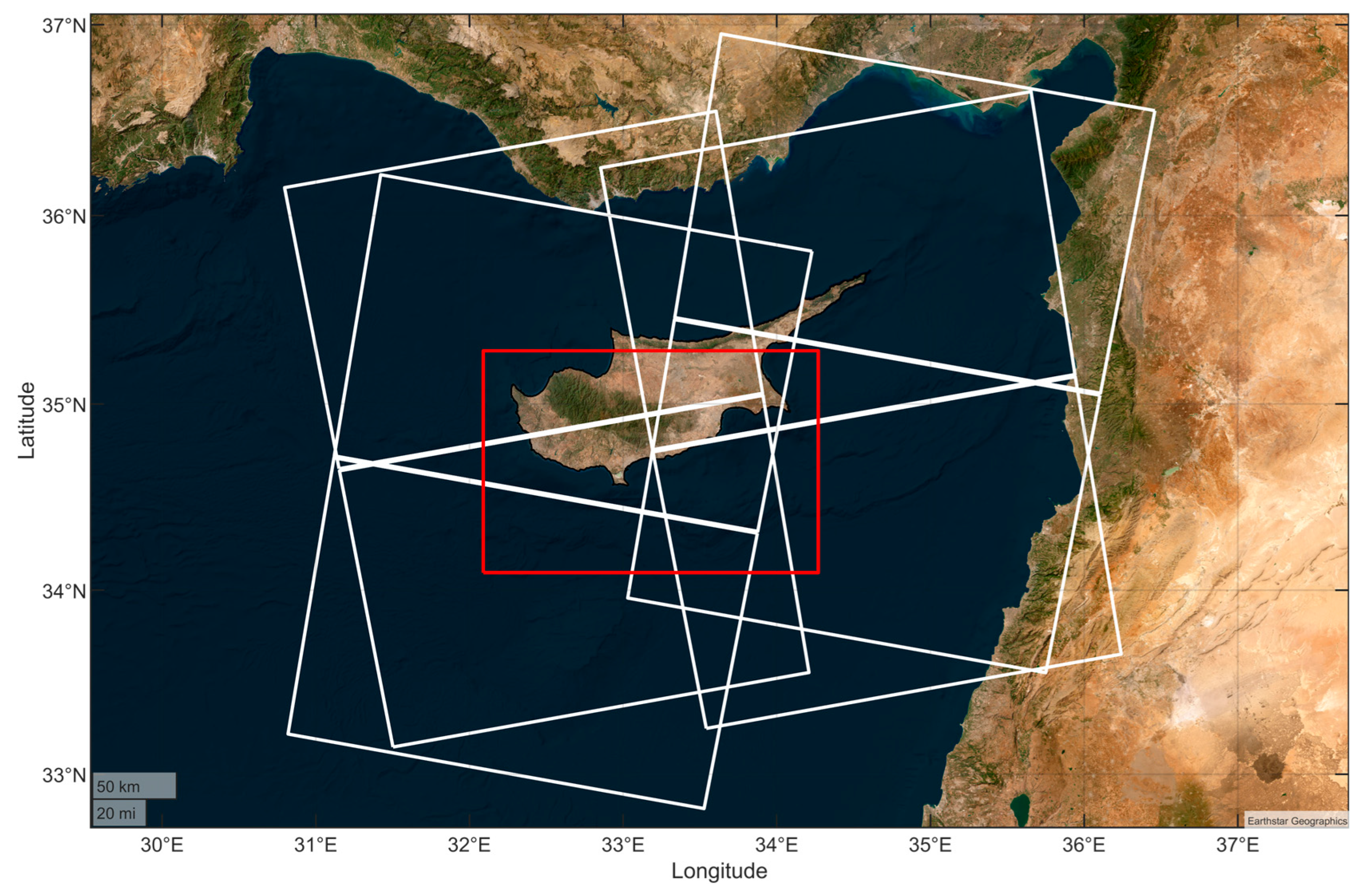
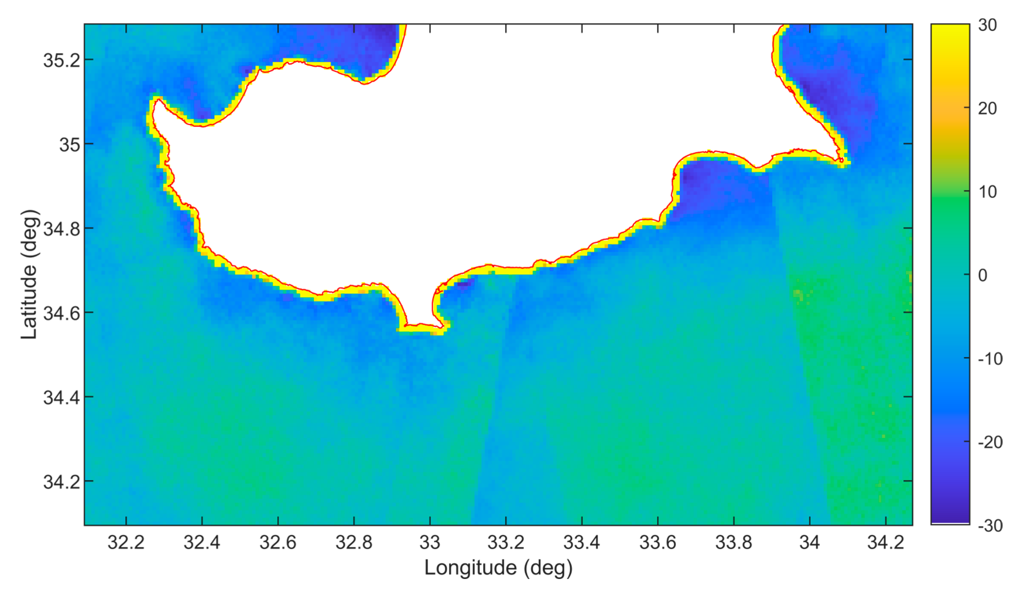
2. Area of Study and Training Datasets

Despite being generalizable to any area of interest and conditions, the method proposed in this study focuses on the offshore area around Cyprus (Figure 1) to simulate wind speed at datetimes when Sentinel-1 information is absent or partly recorded over the study area. As latest statistical indications from the [30] conclude, Cyprus lags in the exploitation of renewable energy sources; thus, remedial steps should be taken in this direction. The remote location of the island further highlights the need for disengagement from fossil fuels, as high dependence on such energy sources has kept electricity cost at peak levels, placing Cyprus among the most expensive EU member states in terms of electricity prices [31]. The dynamic climate conditions due to mesoscale influences in the southeastern Mediterranean region cause variable winds, which are further influenced by the orographic effects of the Cyprus mainland [32]. This fact alone provides an added value to the current work, as typically exploited wind field datasets are unable to identify fine-scale spatial patterns of interannual and intraseasonal variability [33] and accurately assess the wind resources in the study area.
Data consist of image time series from UERRA-HARMONIE [34] regional reanalysis and Sentinel-1 SAR Level-2 OCN datasets [35], which were initially made available at the spatial resolutions of 11 km and 1 km, respectively. As both datasets originally come as gridded products, the study area is discretized into 132 × 242 cells of 0.009° (~1 km), matching the spatial resolution of the finest-scale product (Sentinel-1). Onshore (land) areas of Cyprus where SAR wind retrievals are not available are masked-out. The sample period for both datasets extends from 1 June 2017 to 31 May 2019, encompassing two (2) full season cycles. A visual depiction of the image time series derived from the two data sources is provided in Figure 2.

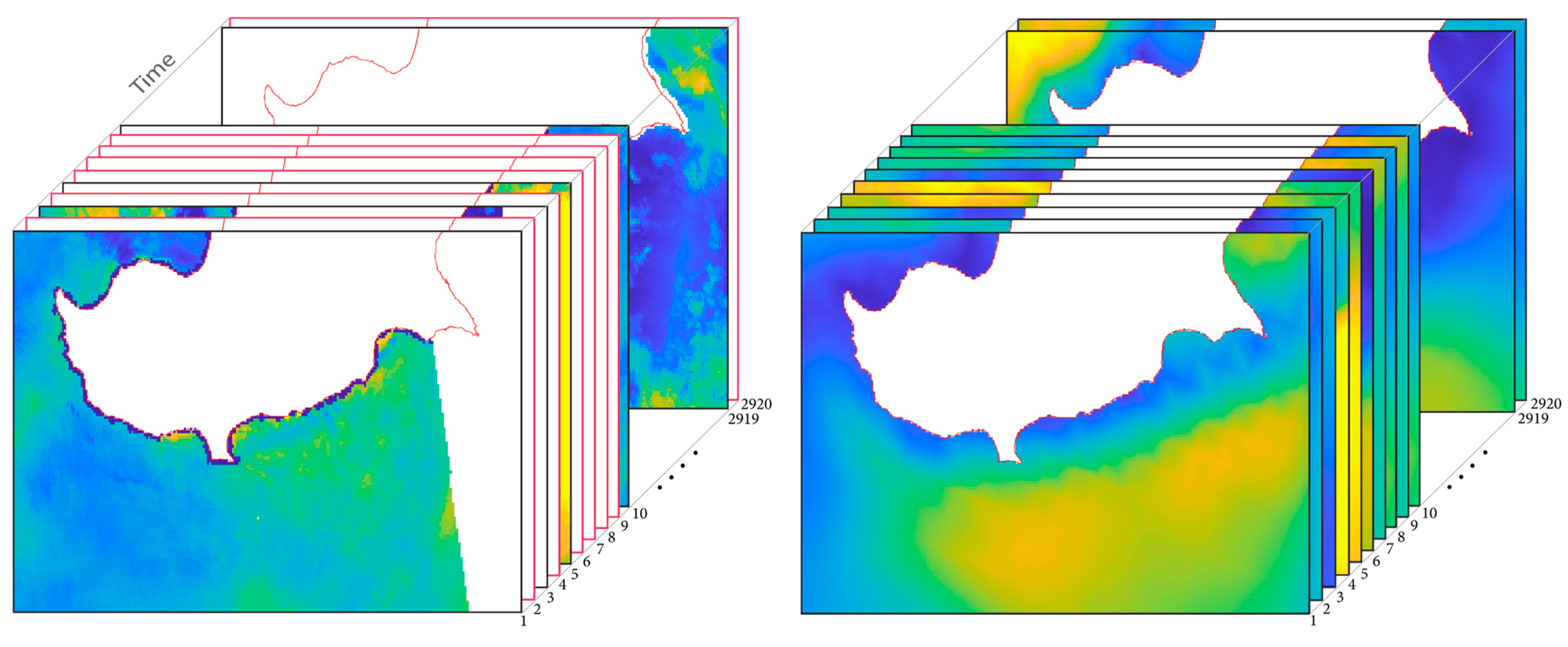
2.1. Sentinel-1A/B SAR Wind Retrievals

The Sentinel-1 near-polar, sun-synchronous-orbiting satellite constellation operates during both day and night to acquire C-band (5.405 GHz) SAR imagery unaffected by daylight and cloud conditions. Each satellite has a 12-day repeat cycle, reducing the combined repeat cycle to 6 days. Satellites share the same orbital plane, albeit with a 180° orbital phasing difference. Sentinel-1 wind retrieval is achieved via the inversion of the estimated NRCS using CMOD-IFR2 GMF by default and a priori wind information obtained from the European Centre for Medium Forecast (ECMWF) atmospheric model. Bayesian inference is then used to estimate the wind vectors in each grid cell [36]. Images in the offshore area around Cyprus are acquired by both satellites in an interferometric wide (IW)-swath mode and under vertical–vertical (VV) + vertical–horizontal (VH) dual polarization operation at approximately 3:45 and 15:45 coordinated universal time (UTC). Therefore, one to two scenes partially cover the study area each day within a 4-day run, leaving 3 days in-between without a scene. The ability of Sentinel-1 C-band SAR instruments to acquire simultaneous co- and cross-polarization imagery, in combination with the fine spatial resolution of the final products, offers a great potential for retrieving the spatial variability of offshore wind at a high level of detail, especially in areas such as coastal waters, where small-scale wind features cannot be revealed by other means [37]. Hence, Sentinel-1 data can serve as primary input for offshore wind resource assessment studies or for the validation of wind speed estimates derived from other data sources (e.g., physical model outputs).
In this work, Sentinel-1 Level-2 OCN products from 483 tiles were acquired in bulk via the Alaska Satellite Facility (ASF). Ocean wind field (OWI) geophysical component data, in particular, refer to fine-spatial-resolution (1 km) ground-range gridded estimates of the surface wind speed a height of 10 m above the sea surface. Sentinel-1 Level 2 OCN wind fields are associated with a quality flag at the pixel level, ranging between 0 and 3 (high to low quality). The flag value communicates the inversion quality but is also related to the geophysical quality of the product, as well as the estimated NRCS quality [38]. Low-quality wing flag values, typically found around the coastline, were completely discarded. Sentinel-1 SAR images also exhibit systematic border noise [39], resulting in artefacts along the east and west image edges. The problematic image rows/columns were completely removed from these images. Sentinel pixel values are resampled to the closest regular square grid node, and a maximum distance of 1 pixel (0.009°) is set to prevent long-distance allocation of remote pixel values. The regular grid-bounding box and Sentinel tiles recorded around the study area within a one-week period are indicated by red and white outlines, respectively, in Figure 1. Tiles tilting to the right occur during descending orbits, whereas tiles tilting to the left occur when the satellites are ascending. The tilting of Sentinel products and the spatial microvariability related to satellite images specify different pseudo-grids for almost every tile.

2.2. UERRA-HARMONIE Regional Reanalysis

Reanalysis methods attempt to provide a comprehensive description of the atmospheric state by reconstructing past weather conditions via a data assimilation scheme. The provision of estimates at each grid point in a region (e.g., Europe) for each regular output time over a long period and always using the same format makes reanalyses very convenient and popular datasets to work with. Regional reanalyses are also produced within the context of the UERRA project and delivered by the Copernicus Climate Change Service. The UERRA-HARMONIE three-dimensional variational data assimilation system delivers pan-European reanalysis gridded data that are made available online by the European Centre for Medium-Range Weather Forecasts (ECMWF) [40]. The selected dataset refers to a single pressure level, providing wind speed estimates at a height of 10 m above the sea surface every 6 h, starting from 00:00 UTC each day and at a horizontal spatial resolution of 11 km. Therefore, UERRA data were also clipped and resampled via linear interpolation to the Sentinel-1 grid to provide both coarse- and fine-scale information in the same spatial domain. Model outputs for the 2-year period between June 2017 and May 2019 are used in this work as auxiliary data, initially for TI selection and subsequently to locally constrain the simulation outputs. It should be stressed here that the Sentinel-1 and UERRA datasets are produced by different means and with different purposes; therefore, they are not considered to represent the same type of information at two different scales. Rather, their complementarity is used to realistically reconstruct the wind speed patterns for the dates and times for which fine-scale information is not available.

3. Methodology

3.1. Multiple-Point Statistical (MPS) Simulation Framework

Geostatistical simulation provides an attractive means of estimating spatiotemporal distributions, taking into consideration local variability, thus avoiding the smoothing effects of kriging interpolation [41]. Falling in the realm of stochastic approaches, simulation aims to produce multiple realizations (2D or 3D synthetic representations) of the considered attribute, thus also providing a measure of spatial uncertainty [42]. However, simulation methods based on two-point (pairwise) measures of spatial heterogeneity, such as variograms or correlograms do not adequately reproduce complex patterns in simulated realizations [43,44] such as those characterizing highly variable climate parameters (e.g., wind and precipitation), nor do they account for non-linear dependencies among multiple variables. Therefore, higher-order statistics are required [45].
MPS, having undergone remarkable progress since their first introduction, replace two-point variograms with training images (TIs). The latter are considered repositories of spatial patterns from which one infers higher-order (multiple-point) statistics, e.g., involving triplets, quadruplets or more complex combinations of attribute values [46,47], without adopting a random function model [48]. MPS can simultaneously account for spatial dependence between attribute values involving multiple points at a time based on higher-order (multiple-point) statistics extracted from TIs, while respecting data; imposing constraints of data fidelity/reproduction is termed conditioning [47]. As natural phenomena, such as wind, present continually recurrent spatial patterns, one or more representative TI can adequately describe a time-varying dataset. Once identified, these patterns can be used in the gap-filling process to simulate the missing information. MPS have been alternatively (to traditional stochastic simulation techniques) exploited to reconstruct complex patterns using samples of historical data, while respecting the spatial variability of the phenomenon under consideration. This data-driven approach falls in the same realm as analog forecasting, the main idea being that weather patterns reoccur in time, and therefore, long-term forecasting of probability distribution functions (PDFs) is feasible using relevant prior information [49]. This is achieved in MPS by computing the conditional probability of joint combinations of attribute values (known as data events) occurring based on patterns contained in the selected TI, such as higher-order (beyond bivariate) statistical dependencies. The conditional cumulative distribution function (CCDF) estimated for the simulation of random variable Z ( x ) at each successive location is expressed as:
F ( z , x | d n ) = P r o b { Z ( x ) z | d n }   ,   d n = { z ( x 1 ) , ,   z ( x n )   } ,
where x is the pixel where simulation is to be performed, and d n represents the data events consisting of z values in the n neighboring pixels (local conditioning; either data or simulated values at previously visited nodes). Pixels are simulated sequentially in a random order called the simulation path. The above formula can be extended to meet the requirements of multivariate cases of m variables as:
F ( z , x | d n 1 1 ,   , d n m m ) = P r o b { Z v ( x ) z | d n 1 1 ,   , d n m m }   ,   v = 1 ,   ,   m
Because different neighborhoods and data events can be defined for each variable ( Z k ), the definition of a joint data event for a simulation node ( x ) involves the computation of lag vectors ( L v ) such as:
d n ( x ) = { d n 1 1 ( x ,   L 1 ) , , d n m m ( x ,   L m )   }
For a single variable, the lag vectors at each node (x) in the simulation path are therefore computed by means of subtraction considering the n closest grid nodes as L = { x 1 x , , x n x } . The distance (dissimilarity) between the simulation grid (SG) and the TI joint data events can be subsequently evaluated as the weighted average of distances/dissimilarities between joint data events for each variable using various metrics (e.g., Euclidean, Manhattan, etc.).

3.2. Quick Sampling (QS) Algorithm

A comprehensive description of existing MPS algorithms is given provided by [50]. Despite the high degree of similarity among the majority of them, they mainly differ in terms of the means extracting and storing the pattern information from the TI [51]. SNESIM [52], ENESIM [46], IMPALA [53] and direct sampling (DS) [54] are the most widespread pixel-based MPS simulation algorithms. The latter abandons the concept of explicitly computing the conditional probability distribution in each sequential step but rather directly samples from the TI. This provides the flexibility to deal with one or multiple continuous and/or categorical variables of any structure while accounting for their complex relationships in a computationally efficient way. However, this efficiency has been proven quite sensitive to the selection of the appropriate distance/dissimilarity threshold best-suited for each application, as well as the fraction of the TI to be scanned [55]. In the same vein, quick sampling (QS) [29] computes a mismatch map between the searched pattern and each location in the TI to determine the k best candidates for the node to be simulated, bypassing the computation of the conditional probability distribution. Like in DS, the mismatch refers to the distance/dissimilarity between the data event contained in the SG and the corresponding data events in the TI. The contribution of QS lies in the decomposition of the distance norms and the computation of the mismatch map using fast Fourier transform (FFT), as well as the optimized partial sorting technique applied for ranking the k best candidates, enabling improved scalability and computational efficiency for the performance of MPS simulations. The construction of a mismatch map for each node in the TI instead of relying on a distance threshold to sample the best candidate allows for the simulation of more representative patterns in constant and predictable computation time. The inherent ability of QS to deal with multiple continuous variables is key in addressing the “weakly constrained gap-filling problem” in our work due to the low temporal sampling frequency of Sentinel-1. A predefined kernel (ki) of any type (e.g., exponential or uniform) can be used in QS to apply a weighting scheme to account for both the spatial (auto)correlation between the simulation node and neighboring node values and to assign relative weights to different variables in the multivariate case. More specifically, the QS algorithm consists of the steps described in Algorithm 1 (Inputs, parameters and pseudocode of the quick sampling (QS) algorithm).
Algorithm 1: Quick Sampling
Inputs and parameters:ti(s): training image(s), di: destination image (or simulation grid), sp: simulation path,
dt: data type, k: number of best candidates, n: number of closest neighbors, ki: kernel
Step 1:For every uninformed node x in the defined path ( s p )
Step 2:Retrieve data event d n ( x ) in the d i within the predefined radius
Step 3:Compute the mismatch map by calculating the distance/dissimilarity between data event d n ( x ) in di and d n ( y ) for every node in ti
Step 4:Rank distances in the mismatch map using quantile sorting to determine the k best candidate(s)
Step 5:Sample among the k best candidates and assign the selected value to node x in the d i

3.3. Parametrization

A full list of mandatory and optional QS parameters is provided in the online documentation of the algorithm available at https://gaia-unil.github.io/G2S/ (accessed 2 December 2022), where the latest open-source distribution of QS is also available. These include parameters that can vary and others that are commonly set for the whole configuration. The former include the number of neighbors (n), the kernel (ki) and the data type (dt), whereas the most important among the global parameters is the number of best candidates (k). The remaining parameters used in this study, namely training images (ti), destination image (di) and simulation path (sp) are described in the following section. The rationale behind the choice of both the individual parameter set for each variable (Table 1) and the global parameters is explained in the remainder of this section.
All the variables included in the model setup are continuous. The data type (dt) for each variable is set to 0, which appropriately adjusts the distance (dissimilarity) metric applied; Euclidean distance is used in this case. One of the most important parameters in QS—and MPS in general—is the number of closest neighbors (n) to be accounted for. As n highly depends on the application at hand, it was defined for UERRA and Sentinel-1 variables via trial and error after simulating a subset of the image time series and calculating mismatch statistics between the reference and simulated Sentinel-1 images. The simulated node is therefore conditioned to a pattern consisting of the 25 closest neighbors for UERRA and the 75 closest neighbors for Sentinel-1. A high number of neighbors is required for Sentinel to adequately characterize a specific pattern due to the complex heterogeneity and variability of wind speed, whereas for UERRA, n must be large enough to represent the large-scale wind speed fluctuations detected in the images to properly condition the simulation on the coarse-scale patterns. The rest of the variables, namely longitude, latitude and distance to the coast, are used in this study to account for the non-stationary nature of the wind speed patterns following previous MPS-related applications [26,28]. This is achieved by defining the position of a simulation node ( x ) in order to guarantee that both the location and the orientation of the wind speed patterns are consistent between the TIs and the simulation output. Therefore, a value of n = 1 is used to restrict the nodes among which the mismatch between di and ti is computed to 1. The spatial continuity of the wind speed patterns and the relative weighting of each variable were considered by defining a radial basis function (RBF) kernel expressed by:
K = w e ( h · d ) 2
where h is the bandwidth parameter adjusting for the relative weighting between large- and small-scale variations, and d is the Euclidean (geographical) distance from the center of the kernel. Higher h values translate into a narrow kernel in which only pixels close to the center can significantly contribute. As bandwidth value increases, the relative weight of distant points increases exponentially. The amplitude of the Kernel was adjusted by defining relative weights ( w ) for each variable, as shown in Table 1. In this study, h was set to 0.001 to account for the gradual decrease in the spatial continuity of the wind speed patterns, whereas a different w value was set for each variable. In the case of Sentinel-1, a weight of 1 was used to account for the complex variability of wind speed. A reduced weight of 0.01 was defined for the UERRA auxiliary variable, whereas a 0.1 weight was defined for the three constant variables in time (latitude, longitude and distance to coast).
The number of best candidates (k) parameter can take any value, including decimals. When k is an integer, the sample is derived from a uniform distribution such that every candidate has an equal probability to be drawn. In the case of non-integer k values, the probabilities are defined as follows: First, k is split into integer (int) and decimal (dec) parts. The number of candidates is then defined as i n t + 1 . Each of the candidates except the last one then has a probability of 1 / k of being selected, whereas the last candidate has a probability proportional to the decimal part, which equals 1 ( 1 / k i n t ) . Using k 1 prevents borrowing of identical patterns from the TI, a phenomenon commonly termed verbatim copying. In this study, the number of k best candidates was set to 1.2 to avoid borrowing of large-scale patterns from the TIs while still selecting among the two candidates with the lowest distance between multivariate patterns. Therefore, the selected candidate is chosen among the 2 best (i.e., those with the lowest distance values in the mismatch map), with probabilities of occurrence of 83.33% and 16.67%, respectively. It should be stressed that the selection of n and ki parameters is based on the sensitivity analysis conducted by [29] and was fine-tuned via the examination of the simulated nodes index for the case study presented here.

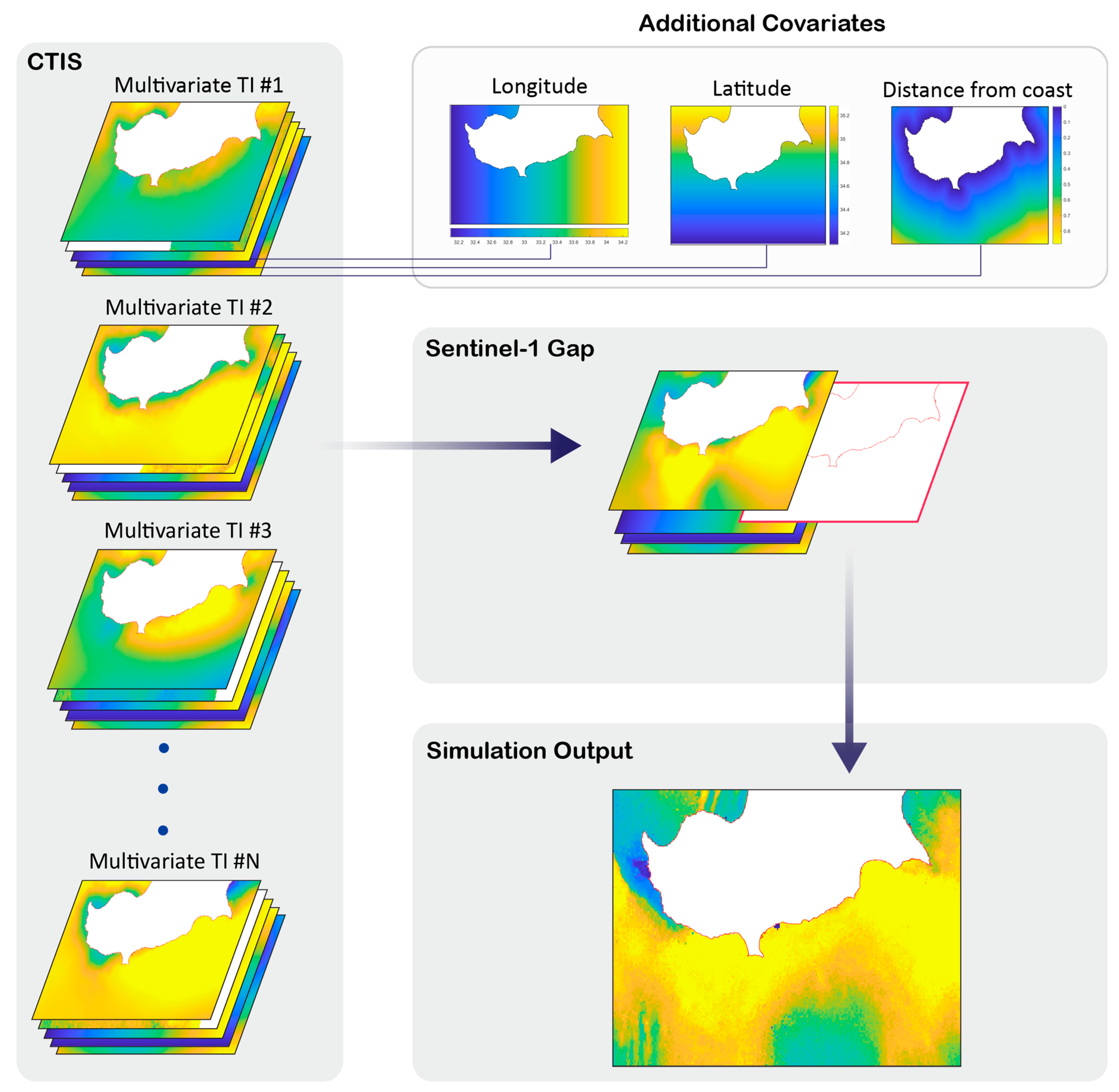
3.4. Conditional Training Image Set (CTIS)

Highly complex wind field spatial patterns reoccur at different times and locations and under different weather conditions within the study region. The non-stationary nature of such structures cannot be modeled or simulated using the complete Sentinel-1 image record but must be reconstructed using a representative sample of the fine-scale satellite imagery. The selected multivariate image set for each gap to be simulated is hereafter termed CTIS. A two-step image classification process was followed in this study to form the CTIS for each gap to be simulated. The first step involves pairing between UERRA and Sentinel-1 training images. To form the UERRA-Sentinel-1 training image pairs while accounting for possible time lags between both datasets, their mismatch within a 12 h time interval is summarized via the root mean square error (RMSE). As UERRA model outputs are available every 6 h, the aforementioned interval involves 3 UERRA images. The UERRA image corresponding to the lowest R M S E is then selected and paired with the informed Sentinel-1 image. Once all the TI pairs have been determined, these are stacked with the rest of the auxiliary variables, namely longitude, latitude and distance from the coast, to form a multivariate TI candidate. The second step involves the computation of R M S E between each pair of UERRA images at Sentinel-1-informed and gap datetimes to identify similar wind speed conditions as those observed in the simulation time steps. Because no Sentinel-1 image is available for these time steps, UERRA is used as a criterion to match the wind speed conditions. The entries of the resulting R M S E matrix are then ranked in ascending order to allow for the selection of Tis, which will form the CTIS at each iteration. A visual example of a CTIS formation is depicted in Figure 3.

3.5. Offshore Wind Speed Image Time Series Simulation

Once Sentinel-UERRA pairs have been formed and the ranked RMSE values between pairs of UERRA images at gap and Sentinel-1-informed datetimes have been generated, the proposed methodology proceeds with TI set selection and the sequential simulation of the missing Sentinel-1 images. As part of the simulation process, the number of training images in the CTIS for each gap to be simulated is determined by an RMSE threshold of 1.5 m/s determined via stepwise optimization on a subset of images.
Despite the threshold set, the number of TIs cannot go below 8 or exceed 13. This range was also determined via trial and error and may vary in different applications depending, among other factors, on the multivariate relationship between the selected variables. Here, having either a lower or higher number of TIs than the aforementioned thresholds can lead to misrepresentation of the fine-scale wind speed patterns to be simulated. Moreover, using a high number of TIs to simulate a single image could significantly increase the computation time without providing added value in terms of the realistic reconstruction of the non-stationary wind fields. If no representative UERRA image can be identified to be used in the CTIS, the gap is not simulated. Once the CTIS has been defined and QS parameters have been set as described in Section 3.3, fine-scale offshore wind speed images are simulated in sequence until all Sentinel-1 image time-series gaps have been filled. Figure 4 provides a step-by-step schematic workflow of the proposed methodological framework.

3.6. Evaluation Metrics

A set of statistical measures were used to evaluate the simulation performance. Sentinel-1-informed images were previously validated [18] against coastal meteorological stations and are thus considered reference data against which the simulation outputs are evaluated. To allow for comparisons between the simulated and reference images, the leave-one (image)-out cross-validation (LOOCV) technique was employed. This evaluation measure refers to the splitting of the dataset into test (used for validation) and training data, the latter of which is used to train the model. In this work, LOOCV refers to leaving an informed Sentinel-1 image out at each iteration and attempting to reconstruct it anew by selecting among the remaining Sentinel-1-informed images to form the CTIS. The process is repeated until all Sentinel-1-informed images are left out once, except when the RMSE threshold is exceeded, in which case image simulation is skipped. The following statistical measures are then used to compare the spatiotemporal distributions of the image time series.

3.6.1. Similarity and Divergence Measures

The Perkins skill score (PSS) and Kullback–Leibler (KL) divergence are used to statistically compare the reference and simulation distributions in each grid cell. The PSS [56] provides a similarity measure by quantifying the overlapping area between two probability density functions (PDFs). This allows for evaluation of the resemblance of the reference distribution by the generated realizations while comparing across entire PDFs. PSS is formulated as follows:
P S S = b = 1 B m i n i m u m ( q b ( x ) , p b ( x ) )
where q b ( x ) and p b ( x ) are the simulation and reference distributions, respectively, and B is the total number of bins. As the PSS provides a calculation of the cumulative minimum value of two distributions by bins, possible values range between 0 and 1, with the former suggesting no overlap between the distributions and the latter indicating a perfect distribution match. KL divergence (or relative entropy), on the other hand, uses the same frequencies on the log scale to quantify the divergence between two probability distributions. This is essentially an indicator of how the two distributions differ or how much information is lost during the attempt to match the reference probability distribution. As opposed to PSS, a KL value of 0 indicates two identical distributions; otherwise, the larger the value, the more different the distributions are supposed to be. KL divergence, in its most common form, is expressed as:
D K L ( p || q ) = b = 1 B p b ( x ) · log ( p b ( x ) q b ( x ) )
Note that D K L ( p || q ) is a non-negative measure. Moreover, zero (0) values in either the reference or simulation distribution would lead to complications in the computation of log ( p b ( x ) q b ( x ) ) . This issue is addressed here by smoothing both distributions via the introduction of a small constant (c ( c = 10 3 )) such as p b ( x ) > 0 and q b ( x ) > 0 . Furthermore, P S S , D K L ( p || q ) and B can vary from one location to another; however, for notational simplicity, we do not explicate the dependence of B on x . Despite being visually presented in the following section in the form of maps, both measures described above implicitly characterize the temporal behavior of wind speed time series in each grid cell. This is particularly important because most applications related to wind resource evaluation focus on cumulative wind resources over specific areas rather than wind speed values at particular time instances.

3.6.2. Spatial Correlation

Experimental (sample) semi-variograms of reference and simulated Sentinel-1 images are compared for the two example dates provided in Section 4. Variograms allow for comparison of spatial correlation (or continuity) of the related structures by quantifying the average similarity among attribute values separated by given distance lags. To examine whether spatial correlation varies with direction, one can compute directional variograms along different directions. Here, both omnidirectional and directional variograms along 90° and 180° directions are computed to evaluate the capability of the proposed method to capture the spatial correlation in the wind speed field on target (training) dates.

3.6.3. Relative Bias (%)

A simple yet useful spatiotemporal metric to evaluate the performance of the simulation technique used in this study is the relative bias (RB) in percent. For every informed Sentinel-1 image, a bias map is computed by subtracting the reference image from the mean of the realizations generated for this datetime at the pixel level. By dividing the result by the reference value and multiplying by 100, we obtain a relative bias for each evaluation time step. The bias associated with each grid cell with respect to the reference value is computed as follows:
R B = i = 1 N ( z ¯ s ( x i ) z ( x i ) ) i = 1 N z ( x i ) · 100
where z ¯ s ( x i ) is the mean of realizations in the i t h grid cell, and z ( x i ) is the corresponding reference wind speed value. This study makes use of the median relative bias (MRB) which refers to the ensemble median of the estimated relative bias maps.

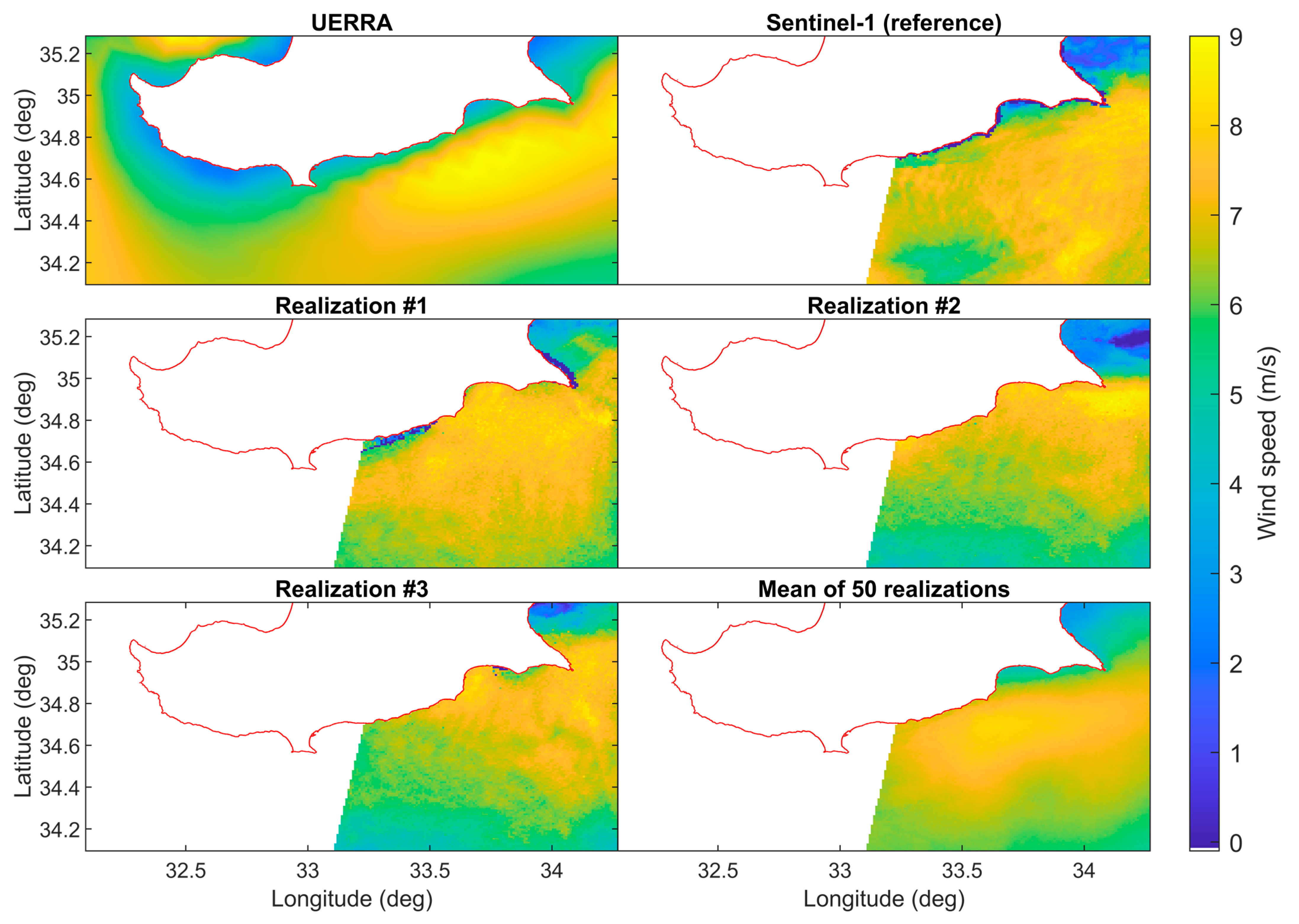
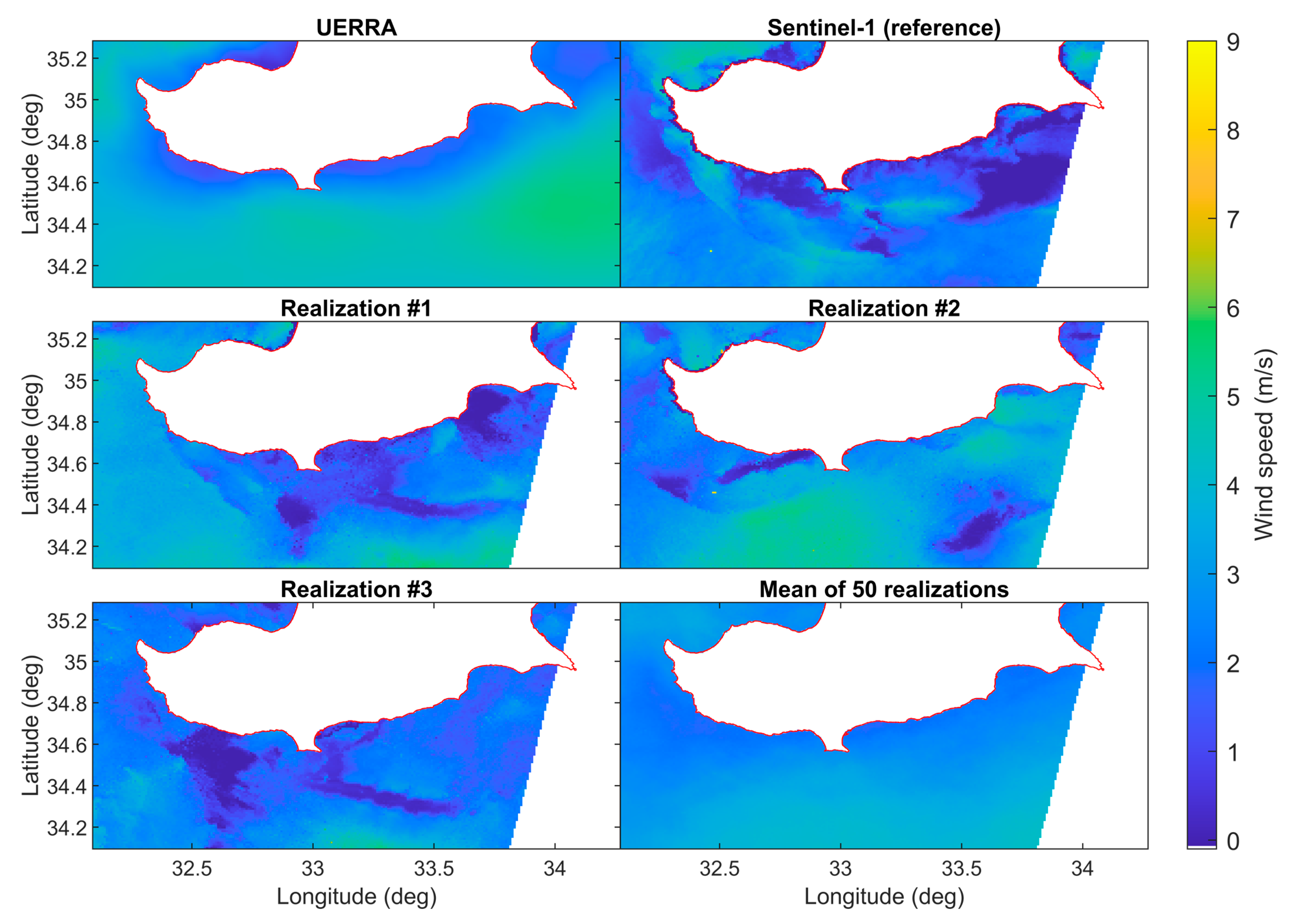
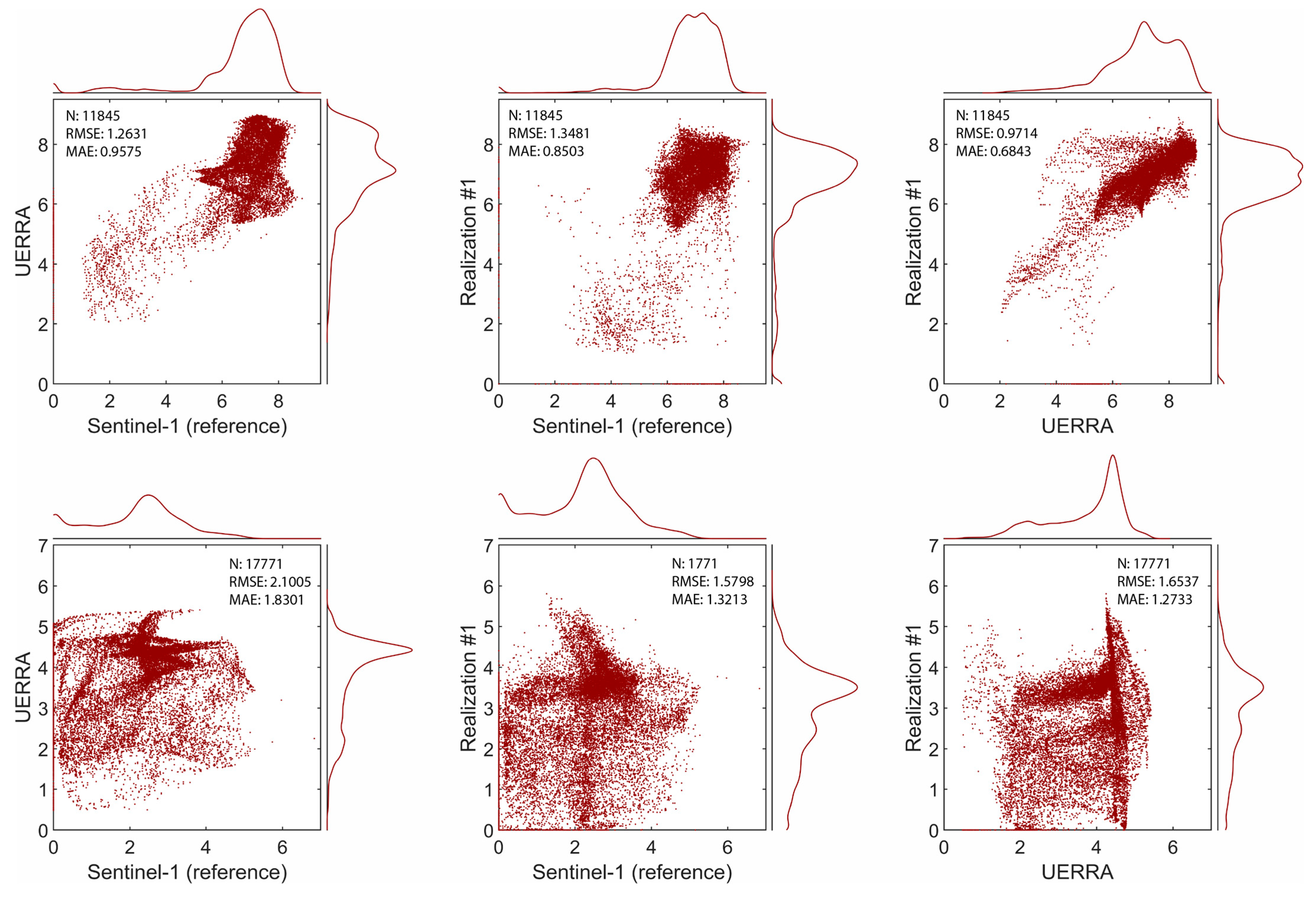
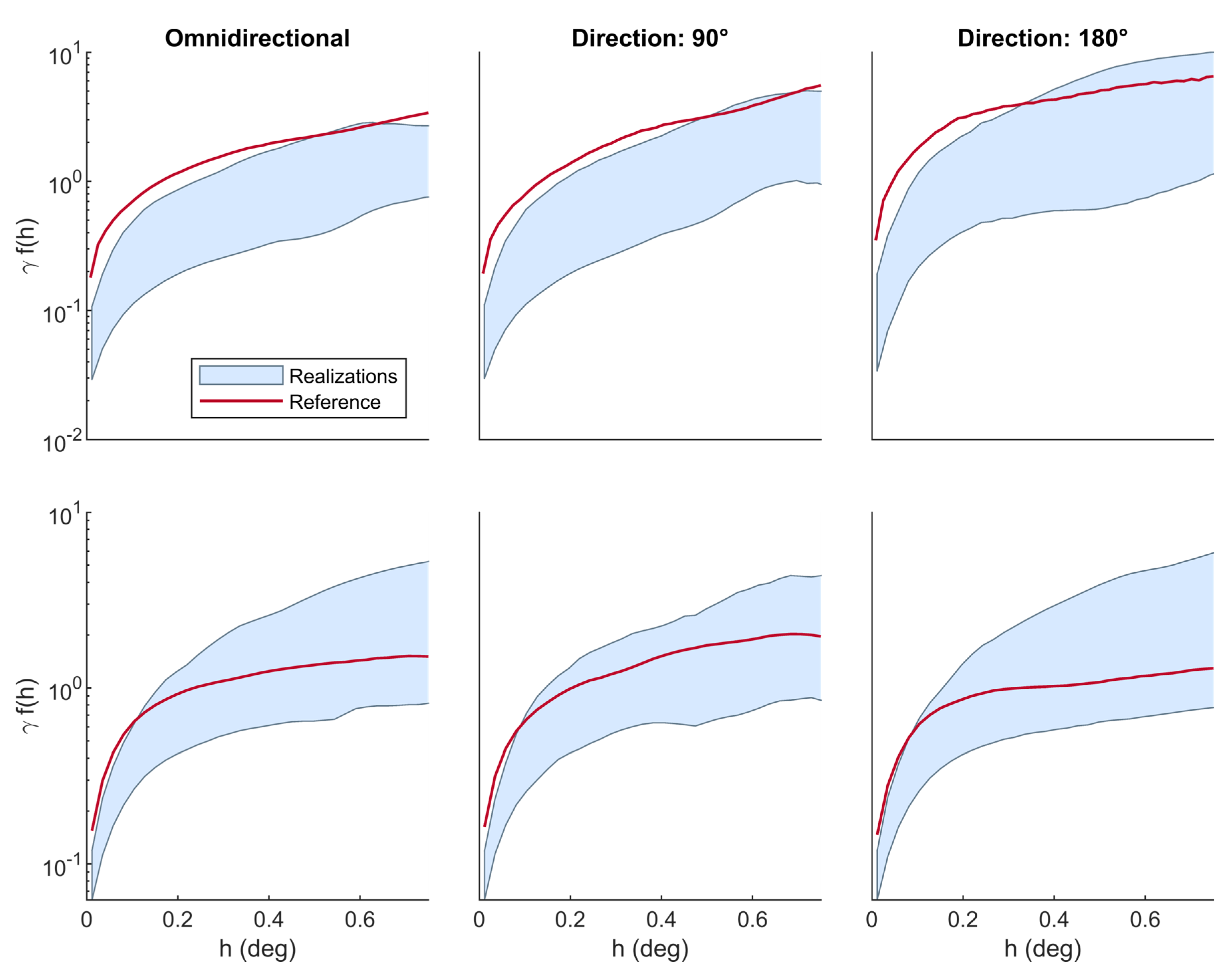
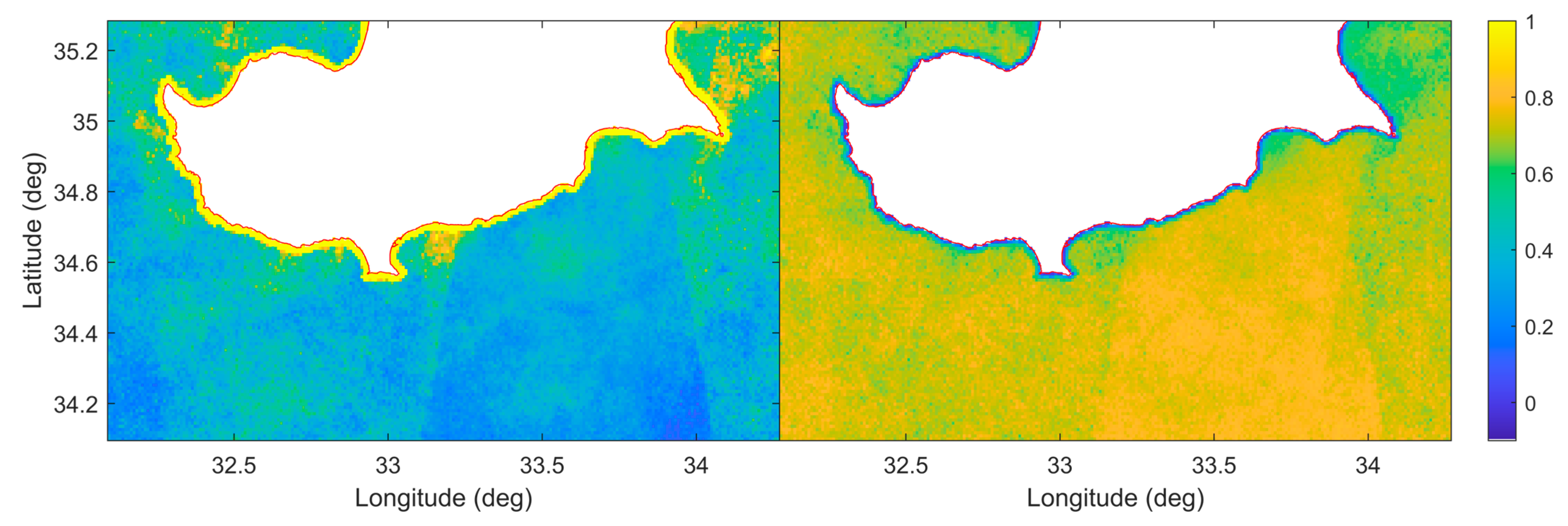
4. Results and Evaluation

A visual comparison between simulated wind fields and reference Sentinel-1 images precedes the statistical comparison using the abovementioned indicators. Two selected examples are demonstrated in Figure 5 and Figure 6 to showcase the ability of the proposed methodology to reconstruct the reference wind speed patterns. The selection of these cases is based on the wind speed pattern structure and variability characterizing the two reference images, which are representative of low-to-moderate and high-intensity wind speed events over the study area. The cases also highlight the ability of MPS and the proposed method to simulate complex spatial patterns. Note that the reference image depicted in the two examples was not included in the training dataset used for the simulation, as this would lead to biased estimates. It is also important to mention here that a larger part of the image is simulated in the second case, in which the Sentinel-1-informed image covers almost the entire area of interest. Therefore, larger-scale wind speed patterns have to be identified in the CTIS and matched by the QS algorithm for the simulation.
Figure 5 depicts an example in which UERRA coarse-scale wind speed patterns spatially cluster in accordance with Sentinel-1 estimates, albeit generally exhibiting slightly higher wind speed values. Therefore, simulated realizations are able to reconstruct the reference spatial variability while reproducing the structure, location and orientation of wind speed patterns. Such realistic patterns are evident in the realizations presented in Figure 5. However, in Figure 6, not only the variability but also the wind speed patterns differ in space between UERRA and Sentinel-1. Whereas wind speed in UERRA is spatially clustered in low- and moderate-wind-speed blobs close to and further from the coast, respectively, Sentinel-1 images present with complex wind speed spatial heterogeneity and no clear structure regarding the wind speed intensity. As the simulation is conditioned to UERRA, this difference is also reflected in the three generated realizations, as well as in the average of the realization ensemble, in which the wind speed intensity appears smooth across the entire area of interest. However, our aim was to reproduce fine-scale wind speed pattern variability and spatiotemporal heterogeneity rather than to recreate the exact reference field, as this also largely depends on the dependence between primary and auxiliary information—Sentinel-1 and UERRA in this case.
The scatterplots and marginal distributions presented in Figure 7 are used to compare the reference and simulated fields, as well as the UERRA auxiliary variable at the same datetimes. The two rows of subfigures refer to the wind speed values derived from the images of the examples presented above. A linear relationship is quite evident in the first example, in which all three variables seem to be pairwise-correlated. In the second example, however, there is no linear correlation between UERRA and the two fine-scale images, and the simulated realization seems to generally overestimate the reference field. This is also confirmed by the accompanying statistics (RMSE and MAE) computed between each pair of wind speed images. Furthermore, the deviation largely originates from the high number of zero (0)-wind-speed values only apparent in the Sentinel-1 image, the existence of which should be further investigated, as they commonly appear in many reference images. A slight overestimation of the reference wind speed values by the realization is evident in both examples, which is also explained by the higher UERRA wind speed values compared to the reference image. It should be noted that points depicted in the scatterplots between the realization and the reference images (second column) are not expected to be aligned on a 1:1 basis, as no reference conditioning data are available. It is anticipated, however, that the correlation (dependence) between UERRA and reference images (first column) is adequately reproduced in the realizations (third column).
In contrast to previous metrics, the spatial dependence expressed in terms of omnidirectional and anisotropic (along 90° and 190° directions) variograms between the reference and simulated wind fields (Figure 8) appears to be better represented in the second example. As previously mentioned, although wind speed patterns are not locally respected, the spatial variability is well reproduced over the study area. The reference experimental variogram thus appears close to the middle of the 5%–95% envelope both for the omni- and the directional realization variograms. However, the corresponding variograms on 10 June 2017 present a slight semi-variance overestimation compared to the reference image, spanning across different ranges according to the direction. A better reproduction of the spatial dependence of the reference wind field by the realizations is evident along the 180° direction in distances greater than 0.3 degrees. Furthermore, there is small-scale variability for negligibly small distances in the reference variograms of both dates, a phenomenon that is commonly termed a nugget effect in geostatistics. Because the simulated fields are conditioned to UERRA coarse-scale patterns, they cannot easily reconstruct this variability in such small distances. As the distance increases, however, the reconstruction appears to better reproduce the reference spatial variability. Nonetheless, realizations seem to generally respect the spatial dependence characterizing Sentinel-1 wind speed images.
Kullback–Leibler divergence and Perkins skill score plots (Figure 9) also indicate an overall convergence between the reference and simulation distributions. Both metrics were computed over the full reference and simulation image time series (461 images). The highest KL values (and lowest PSS values) are observed around the northeast edge of the study area, where pattern matches are limited by the spatially discontinuous subdomain due to Cyprus mainland and edge effects. Moreover, the substantial number of missing values close to the coast (discarded due to low-quality flag values) does not allow for an efficient reconstruction. Conversely, the highest number of Sentinel-1 nodes is within the area enclosed by the sharp edges evident in the east of the study area. There, both metrics indicate a better agreement between the two distributions in comparison to the rest of the domain, indicating the potential for the reconstruction of longer time series as more Sentinel-1-informed images become available.
The sharp boundaries due to the difference of Sentinel-1 samples in each node are more evident in Figure 10, which depicts the median relative bias plot. Whereas KL and PSS plots were computed by per-pixel comparisons of the distributions in time, the MRB plot results from the subtraction of the reference and simulation spatial distributions at each simulation time step. This is more useful to assess the reconstruction of the reference wind fields in space. In general, an overestimation of the reference spatial distribution by the simulation can be concluded. The opposite is true for the northern areas of the domain, especially close to the coastline. The southeastern part of the study area, where the fewest Sentinel-1-informed nodes reside, presents the highest positive bias of the order of 5–10%. Nevertheless, the bias ranges between −5 and 0% in most of the study area, indicating a relatively low MRB between the reference and the mean of 50 realizations at each simulation time step.

5. Discussion

5.1. Challenges and Emerging Opportunities

QS—and MPS in general—attempts to reconstruct image patterns by resampling values from the available training dataset. The simulation of values beyond the range of the TIs is thus not possible without involving parametric approaches [57]. This makes the algorithm inefficient when called to simulate extreme or rare events, as the pool of relative values in the TI set is small. A longer image time series including more representative values for every class would eventually lead to a better representation of infrequent wind speed patterns and more accurate image reconstructions by the proposed technique. Sentinel-1 satellites already count more than 5 years of lifetime providing fine-spatial-resolution wind speed estimates on a global scale. The resulting image time series can serve as primary data in the proposed simulation framework to provide realistic reconstruction of the wind speed patterns in time instances for which no information is available. It should be stressed that the examples provide a demonstration of the ability of the proposed method to simulate wind speed patterns at fine spatial resolution while reproducing the fine-scale variability of the reference fields. As the study area grows and Sentinel-1 continues spanning the earth, more TIs and therefore more patterns will be available to avoid wind field gaps where they exist.
Apart from the long-term statistical outputs, intermittency is also important when assessing the wind speed and, more importantly, the wind energy potential. Although a seasonal analysis goes beyond the scope of this study, it could further reveal how well the proposed methodology can reproduce the wind speed conditions in each season. A deeper study of the physical processes driving the wind fields would shed light on the reoccurrence of wind speed patterns, which is crucial for selecting the appropriate TIs. However, given that Sentinel-1 SAR can only provide estimates of near-surface wind fields, no safe conclusions can be drawn regarding the variations in wind speed at different pressure levels (i.e., upper-level and turbine-height level). For example, diurnal cycles are known to vary depending on the height, although offshore sites tend to exhibit less significant variations [58]. Although various techniques have been applied to extrapolate near-surface offshore wind speed at different heights using mathematical functions [59,60,61], diurnal variations at different altitudes cannot be resolved in such datasets.
The fact that Sentinel-1 (reference) images in the examples presented in Section 4 are only partially informed over the study area makes the reconstruction of such fine-scale wind speed fields even more challenging. The resulting spatially discontinuous fields do not offer a complete set of possible pattern matches, especially when searching within a defined radius. A possible solution would be to extend the spatial domain of interest, although this would lead to an increase in the computation time linearly analogous to the increase in SG size and following a power function of n log ( n ) with respect to the increase in TI size [29]. Low correlation between UERRA and Sentinel-1 pairs in the formed CTIS due to inconsistent wind speed patterns can also lead to poor simulation performance. The simulated fields in such cases mostly follow the structure of the coarse-spatial-resolution product. However, the spatial variability of Sentinel-1 images can be reproduced well in the simulated images.
Lastly, the proposed framework uses a configuration that has been fine-tuned for the specific area of interest and conditions. Although the method is flexible enough to be employed in any region, both the method and QS setup should be adapted to the selected area of interest after careful consideration of the climate conditions.

5.2. Alternative Auxiliary Data Sources

A plethora of regional and global reanalysis datasets at different temporal and spatial resolutions exists. Once validated against more accurate measurements, such auxiliary datasets can be used alone or combined in the proposed simulation framework. This will allow for the selection of the most informative long-term dataset to supplement the fine-scale Sentinel-1 SAR information and subsequently lead to better-informed simulation outputs. Nevertheless, the proposed method of TI selection to form the CTIS for the simulation of each datetime gap appears to be quite efficient despite the bias between Sentinel-1 and UERRA images. The use of additional covariates that may possess high correlation with wind speed (e.g., elevation and temperature) can also be investigated, although this may prove computationally demanding. Highly correlated variables may also be involved in the process of TI selection and the formation of the CTIS. A weather classification technique can be also applied once the appropriate climate variables have been defined and used as auxiliary data. A similar approach was carried out in [28].

6. Conclusions

In this work, we propose a novel geostatistical simulation framework to reconstruct fine-scale offshore wind speed patterns and gap fill Sentinel-1 image time series. The proposed method is based on a statistical classification scheme for TI selection and an MPS algorithm, namely QS, to generate multiple wind field realizations on time instances for which relevant Sentinel-1 information is not available. Evaluation results highlight the ability of the proposed method to realistically simulate wind speed patterns at fine spatial resolution while reproducing the reference variability. Based on our analysis, we conclude that the simulation performance using the technique proposed herein can be further improved. The formation of a CTIS for each simulated gap rather than using the complete image time series as TIs has been proven efficient to adequately characterize the spatial heterogeneity of the underlying wind fields. This technique can also be employed to simulate similarly complex spatial fields (e.g., rainfall) exhibiting non-linear multivariate dependencies.
The overarching objective of a resource assessment is to accurately assess wind energy potential and identify potential hot spots for wind farms siting within an area of interest. This involves the fitting of statistical distributions known to follow wind speed time series, e.g., Weibull and gamma, the parameters of which are used for wind power density estimation. Therefore, future work will focus on taking advantage of the simulated fine-spatial-resolution wind speed time series to estimate the wind power potential in the offshore area around Cyprus and identify hot spots for wind farm project development. Once clusters of high wind speed are identified, local assessment and feasibility analysis will be conducted to assist micrositing studies. Short-term wind speed forecasting using the proposed simulation framework can also be employed to inform current coarse-scale datasets. Seasonal analyses, along with intermittent energy storage plans, will additional areas of future focus.

Author Contributions

Conceptualization, S.H., G.M. and P.K.; methodology, S.H. and G.M.; validation, S.H., G.M. and P.K.; formal analysis, S.H.; investigation, S.H., G.M. and P.K.; resources, S.H., P.K. and G.M.; data curation, S.H.; writing—original draft preparation, S.H.; writing—review and editing, S.H., G.M. and P.K.; visualization, S.H.; supervision, G.M. and P.K.; project administration, S.H., G.M. and P.K.; funding acquisition, S.H. All authors have read and agreed to the published version of the manuscript.

Funding

This research was partially funded by the Swiss Federal Commission for Scholarships for Foreign Students (FCS) via Swiss Government Excellence Research Scholarships (ESKAS-Nr: 2020.0314).

Acknowledgments

The authors would like to thank Mathieu Gravey for his support in the use of the quick sampling (QS) algorithm.

Conflicts of Interest

The authors declare no conflict of interest.

Nomenclature

x Pixel location in the simulation grid
y Pixel location in the training image
F ( · ) Conditional cumulative distribution function (CCDF)
Z ( x ) Random variable at location x
z Outcome of random variable Z , an attribute value
n Subscript indicating the number of neighboring pixels
iSubscript indicating the index of a pixel over the entire image
d n Data event ( z values) of n neighboring pixels
L Lag vectors of data events
m Superscript indicating multiple variables
v Variable index
hKernel bandwidth (degrees)
dEuclidean distance from kernel center (degrees)
w Relative variable weight
D K L ( p || q ) Kullback–Leibler divergence (relative entropy) from q to p
p b ( x ) Reference distribution for b t h bin at location x
q b ( x ) Simulation distribution for b t h bin at location x
B Number of bins
bSubscript indicating the index of a bin
z ¯ s ( x i ) Mean of realizations at i t h grid cell
z ( x i ) Reference attribute value at i t h grid cell
N Number of pixels over the entire image

Abbreviations

SARSynthetic aperture radar
MPSMultiple-point statistics
NWPNumerical weather prediction
SCATScatterometers
GMFGeophysical model function
NRCSNormalized radar cross section
WRFWeather research and forecasting
TITraining image
CTISConditional training image set
UERRAUncertainties in ensembles of regional reanalyses
QSQuick sampling
EUEuropean Union
ECMWFEuropean Centre for Medium Forecast
IWInterferometric wide
VVVertical–vertical
VHVertical–horizontal
UTCCoordinated universal time
ASFAlaska Satellite Facility
OWIOcean wind fields
PDFProbability distribution function
CCDFConditional cumulative distribution function
SGSimulation grid
DSDirect sampling
FFTFast Fourier transform
RBFRadial basis function
RMSERoot mean square error
MAEMean absolute error
LOOCVLeave-one-out cross validation
PSSPerkins skill score
KLKullback–Leibler
MRBMedian relative bias

References

  1. GWEC Global Wind Report 2021|Global Wind Energy Council. Available online: https://gwec.net/global-wind-report-2021/ (accessed on 24 September 2021).
  2. WindEurope. Offshore Wind in Europe—Key Trends and Statistics 2020; WindEurope: Brussels, Belgium, 2021; Volume 3. [Google Scholar]
  3. Al-Yahyai, S.; Charabi, Y.; Gastli, A. Review of the Use of Numerical Weather Prediction (NWP) Models for Wind Energy Assessment. Renew. Sustain. Energy Rev. 2010, 14, 3192–3198. [Google Scholar] [CrossRef]
  4. Gryning, S.E.; Floors, R. Investigating Predictability of Offshore Winds Using a Mesoscale Model Driven by Forecast and Reanalysis Data. Meteorol. Z. 2020, 29, 117–130. [Google Scholar] [CrossRef]
  5. Bailey, B.H. Wind Resources for Offshore Wind Farms: Characteristics and Assessment. In Offshore Wind Farms: Technologies, Design and Operation; Ng, C., Ran, L., Eds.; Woodhead Publishing: Sawston, UK, 2016; pp. 29–58. ISBN 9780081007808. [Google Scholar]
  6. Olsen, B.T.; Hahmann, A.N.; Sempreviva, A.M.; Badger, J.; Jørgensen, H.E. An Intercomparison of Mesoscale Models at Simple Sites for Wind Energy Applications. Wind Energ. Sci. 2017, 2, 211–228. [Google Scholar] [CrossRef] [Green Version]
  7. Castorrini, A.; Gentile, S.; Geraldi, E.; Bonfiglioli, A. Increasing Spatial Resolution of Wind Resource Prediction Using NWP and RANS Simulation. J. Wind Eng. Ind. Aerodyn. 2021, 210, 104499. [Google Scholar] [CrossRef]
  8. Optis, M.; Kumler, A.; Brodie, J.; Miles, T. Quantifying Sensitivity in Numerical Weather Prediction-Modeled Offshore Wind Speeds through an Ensemble Modeling Approach. Wind Energy 2021, 24, 957–973. [Google Scholar] [CrossRef]
  9. Karagali, I.; Badger, M.; Hasager, C. Spaceborne Earth Observation for Offshore Wind Energy Applications; Institute of Electrical and Electronics Engineers (IEEE): Piscataway, NJ, USA, 2021; pp. 172–175. [Google Scholar]
  10. Cameron, I.; Lumsdon, P.; Walker, N.; Woodhouse, I. Synthetic Aperture Radar for Offshore Wind Resource Assessment and Wind Farm Development in the UK. In Proceedings of the SEASAR 2006: Advances in SAR Oceanography from ENVISAT and ERS Missions, Frascati, Italy, 23–26 January 2006. [Google Scholar]
  11. Furevik, B.R.; Espedal, H.A.; Hamre, T.; Hasager, C.B.; Johannessen, O.M.; Jørgensen, B.H.; Rathmann, O. Satellite-Based Wind Maps as Guidance for Siting Offshore Wind Farms. Wind Eng. 2016, 27, 327–338. [Google Scholar] [CrossRef]
  12. Ahsbahs, T.; Badger, M.; Volker, P.; Hansen, K.S.; Hasager, C.B. Applications of Satellite Winds for the Offshore Wind Farm Site Anholt. Wind Energy Sci. 2018, 3, 573–588. [Google Scholar] [CrossRef] [Green Version]
  13. Ahsbahs, T.; MacLaurin, G.; Draxl, C.; Jackson, C.R.; Monaldo, F.; Badger, M. US East Coast Synthetic Aperture Radar Wind Atlas for Offshore Wind Energy. Wind Energy Sci. 2020, 5, 1191–1210. [Google Scholar] [CrossRef]
  14. Schulz-Stellenfleth, J.; Djath, B. Hereon SAR Observations of Offshore Windfarm Wakes. In Handbook of Wind Energy Aerodynamics; Stoevesandt, B., Schepers, G., Fuglsang, P., Yuping, S., Eds.; Springer International Publishing: Cham, Switzerland, 2021; pp. 1–33. ISBN 978-3-030-05455-7. [Google Scholar]
  15. Zhang, B.; Mouche, A.; Lu, Y.; Perrie, W.; Zhang, G.; Wang, H. A Geophysical Model Function for Wind Speed Retrieval from C-Band HH-Polarized Synthetic Aperture Radar. IEEE Geosci. Remote Sens. Lett. 2019, 16, 1521–1525. [Google Scholar] [CrossRef]
  16. Bruun Christiansen, M.; Koch, W.; Horstmann, J.; Bay Hasager, C.; Nielsen, M. Wind Resource Assessment from C-Band SAR. Remote Sens. Environ. 2006, 105, 68–81. [Google Scholar] [CrossRef]
  17. Beaucage, P.; Bernier, M.; Member, S.; Lafrance, G.; Choisnard, J. Regional Mapping of the Offshore Wind Resource: Towards a Significant Contribution from Space-Borne Synthetic Aperture Radars. IEEE J. Sel. Top. Appl. Earth Obs. Remote Sens. 2008, 1, 48–56. [Google Scholar] [CrossRef]
  18. Hadjipetrou, S.; Liodakis, S.; Sykioti, A.; Katikas, L.; Park, N.-W.; Kalogirou, S.; Akylas, E.; Kyriakidis, P. Evaluating the Suitability of Sentinel-1 SAR Data for Offshore Wind Resource Assessment around Cyprus. Renew. Energy 2022, 182, 1228–1239. [Google Scholar] [CrossRef]
  19. Majidi Nezhad, M.; Heydari, A.; Groppi, D.; Cumo, F.; Astiaso Garcia, D. Wind Source Potential Assessment Using Sentinel 1 Satellite and a New Forecasting Model Based on Machine Learning: A Case Study Sardinia Islands. Renew. Energy 2020, 155, 212–224. [Google Scholar] [CrossRef]
  20. De Montera, L.; Remmers, T.; O’Connell, R.; Desmond, C. Validation of Sentinel-1 Offshore Winds and Average Wind Power Estimation around Ireland. Wind Energy Sci. 2020, 5, 1023–1036. [Google Scholar] [CrossRef]
  21. Bourassa, M.A.; Meissner, T.; Cerovecki, I.; Chang, P.; Dong, X.; De Chiara, G.; Donlon, C.; Dukhovskoy, D.; Elya, J.; Fore, A.; et al. Remotely Sensed Winds and Wind Stresses for Marine Forecasting and Ocean Modeling. Front. Mar. Sci. 2019, 6, 443. [Google Scholar] [CrossRef] [Green Version]
  22. Yi, Y.; Johnson, J.T.; Wang, X. On the Estimation of Wind Speed Diurnal Cycles Using Simulated Measurements of CYGNSS and ASCAT. IEEE Geosci. Remote Sens. Lett. 2019, 16, 168–172. [Google Scholar] [CrossRef]
  23. Lu, J.; Ren, K.; Li, X.; Zhao, Y.; Xu, Z.; Ren, X. From Reanalysis to Satellite Observations: Gap-Filling with Imbalanced Learning. Geoinformatica 2021, 26, 397–428. [Google Scholar] [CrossRef]
  24. Mariethoz, G.; McCabe, M.F.; Renard, P. Spatiotemporal Reconstruction of Gaps in Multivariate Fields Using the Direct Sampling Approach. Water Resour. Res. 2012, 48, 1–13. [Google Scholar] [CrossRef] [Green Version]
  25. Jha, S.K.; Mariethoz, G.; Evans, J.P.; McCabe, M.F. Demonstration of a Geostatistical Approach to Physically Consistent Downscaling of Climate Modeling Simulations. Water Resour. Res. 2013, 49, 245–259. [Google Scholar] [CrossRef] [Green Version]
  26. Jha, S.K.; Mariethoz, G.; Evans, J.; McCabe, M.F.; Sharma, A. A Space and Time Scale-Dependent Nonlinear Geostatistical Approach for Downscaling Daily Precipitation and Temperature. Water Resour. Res. 2015, 51, 6244–6261. [Google Scholar] [CrossRef]
  27. Yin, G.; Mariethoz, G.; McCabe, M.F. Gap-Filling of Landsat 7 Imagery Using the Direct Sampling Method. Remote Sens. 2017, 9, 12. [Google Scholar] [CrossRef] [Green Version]
  28. Oriani, F.; Ohana-Levi, N.; Marra, F.; Straubhaar, J.; Mariethoz, G.; Renard, P.; Karnieli, A.; Morin, E. Simulating Small-Scale Rainfall Fields Conditioned by Weather State and Elevation: A Data-Driven Approach Based on Rainfall Radar Images. Water Resour. Res. 2017, 53, 8512–8532. [Google Scholar] [CrossRef]
  29. Gravey, M.; Mariethoz, G. QuickSampling v1.0: A Robust and Simplified Pixel-Based Multiple-Point Simulation Approach. Geosci. Model Dev. 2020, 13, 2611–2630. [Google Scholar] [CrossRef]
  30. European Commission Renewable Energy Statistics: Statistics Explained. Available online: https://ec.europa.eu/eurostat/statistics-explained/index.php/Renewable_energy_statistics%0Awww.irena.org/Publications%0Ahttps://ec.europa.eu/eurostat/statistics-explained/index.php/Renewable_energy_statistics%0Awww.irena.org/Publications (accessed on 22 February 2022).
  31. Eurostat Electricity Price Statistics—Statistics Explained. Available online: https://ec.europa.eu/eurostat/statistics-explained/index.php/Electricity_price_statistics (accessed on 16 December 2021).
  32. Soukissian, T.; Karathanasi, F.; Axaopoulos, P.; Voukouvalas, E.; Kotroni, V. Offshore Wind Climate Analysis and Variability in the Mediterranean Sea. Int. J. Climatol. 2018, 38, 384–402. [Google Scholar] [CrossRef]
  33. Barbariol, F.; Davison, S.; Falcieri, F.M.; Ferretti, R.; Ricchi, A.; Sclavo, M.; Benetazzo, A. Wind Waves in the Mediterranean Sea: An ERA5 Reanalysis Wind-Based Climatology. Front. Mar. Sci. 2021, 8, 1615. [Google Scholar] [CrossRef]
  34. Copernicus climate change service (C3S). Documentation of the RRA System: UERRA. Available online: https://cds.climate.copernicus.eu/cdsapp#!/dataset/reanalysis-uerra-europe-complete?tab=doc (accessed on 21 February 2022).
  35. ESA Sentinel-1—Missions—Sentinel Online. Available online: https://sentinel.esa.int/web/sentinel/missions/sentinel-1 (accessed on 22 December 2021).
  36. Mouche, A. Sentinel-1 Ocean Wind Fields (OWI) Algorithm Definition. Available online: https://sentinels.copernicus.eu/documents/247904/3861173/DI-MPC-IPF-OWI_2_1_OWIAlgorithmDefinition.pdf/dc452ea7-cb37-c227-ac74-0c07a3fb714a?t=1644835258554 (accessed on 14 October 2022).
  37. Hasager, C.B. Offshore Winds Mapped from Satellite Remote Sensing. Wiley Interdiscip. Rev. Energy Environ. 2014, 3, 594–603. [Google Scholar] [CrossRef] [Green Version]
  38. Vincent, P.; Bourbigot, M.; Johnsen, H.; Piantanida, R.; Poullaouec, J.; Hajduch, G. Sentinel-1 ESA Unclassified for Official Use Sentinel-1 Product Specification. Available online: https://sentinel.esa.int/documents/247904/1877131/Sentinel-1-Product-Specification (accessed on 22 February 2022).
  39. Ali, I.; Cao, S.; Naeimi, V.; Paulik, C.; Wagner, W. Methods to Remove the Border Noise from Sentinel-1 Synthetic Aperture Radar Data: Implications and Importance for Time-Series Analysis. IEEE J. Sel. Top. Appl. Earth Obs. Remote Sens. 2018, 11, 777–786. [Google Scholar] [CrossRef] [Green Version]
  40. Copernicus climate change service (C3S). UERRA Data User Guide. Available online: https://cds.climate.copernicus.eu/cdsapp#!/dataset/reanalysis-uerra-europe-complete?tab=doc (accessed on 14 December 2021).
  41. Chilès, J.P.; Delfiner, P. Geostatistics: Modeling Spatial Uncertainty: Second Edition; Wiley-Blackwell: Hoboken, NJ, USA, 2012; ISBN 9780470183151. [Google Scholar]
  42. Atkinson, P.M.; Lloyd, C.D. Geostatistical Models and Spatial Interpolation. Handb. Reg. Sci. 2014, 1461–1476. [Google Scholar] [CrossRef]
  43. Hashemi, S.; Javaherian, A.; Ataee-pour, M.; Khoshdel, H. Two-Point versus Multiple-Point Geostatistics: The Ability of Geostatistical Methods to Capture Complex Geobodies and Their Facies Associations—An Application to a Channelized Carbonate Reservoir, Southwest Iran. J. Geophys. Eng. 2014, 11, 065002. [Google Scholar] [CrossRef]
  44. Tahmasebi, P. Multiple Point Statistics: A Review. In Handbook of Mathematical Geosciences: Fifty Years of IAMG; Daya Sagar, B.S., Cheng, Q., Agterberg, F., Eds.; Springer International Publishing: Cham, Switzerland, 2018; pp. 613–643. ISBN 9783319789996. [Google Scholar]
  45. Journel, A.G. Beyond Covariance: The Advent of Multiple-Point Geostatistics. In Geostatistics Banff 2004; Springer: Dordrecht, The Netherlands, 2004; pp. 225–233. [Google Scholar] [CrossRef]
  46. Guardiano, F.B.; Srivastava, R.M. Multivariate Geostatistics: Beyond Bivariate Moments. In Geostatistics Troia ’92; Springer: Dordrecht, The Netherlands, 1993; Volume 1, pp. 133–144. [Google Scholar] [CrossRef]
  47. Strebelle, S. Multiple-Point Geostatistics: From Theory to Practice. Proc. Geostats 2012, 2012, 1–9. [Google Scholar]
  48. Hu, L.Y.; Chugunova, T. Multiple-Point Geostatistics for Modeling Subsurface Heterogeneity: A Comprehensive Review. Water Resour. Res. 2008, 44, 1–14. [Google Scholar] [CrossRef]
  49. Lorenz, E. Atmospheric Predictability as Revealed by Naturally Occurring Analogues. Available online: https://www.semanticscholar.org/paper/Atmospheric-Predictability-as-Revealed-by-Naturally-Lorenz/515deec4e011ebeb02c3f356380dbbc010417b30 (accessed on 14 April 2022).
  50. Mariethoz, G.; Caers, J. Multiple-Point Geostatistics: Stochastic Modeling with Training Images; John Wiley & Sons: Hoboken, NJ, USA, 2014; pp. 1–364. [Google Scholar] [CrossRef]
  51. Grana, D.; Azevedo, L. Subsurface Geostatistical Modeling, 2nd ed.; Elsevier Inc.: Amsterdam, The Netherlands, 2021; ISBN 9780124095489. [Google Scholar]
  52. Strebelle, S. Conditional Simulation of Complex Geological Structures Using Multiple-Point Statistics. Math. Geol. 2002, 34, 1–21. [Google Scholar] [CrossRef]
  53. Straubhaar, J.; Renard, P.; Mariethoz, G.; Froidevaux, R.; Besson, O. An Improved Parallel Multiple-Point Algorithm Using a List Approach. Math. Geosci. 2011, 43, 305–328. [Google Scholar] [CrossRef]
  54. Mariethoz, G.; Renard, P.; Straubhaar, J. The Direct Sampling Method to Perform Multiple-Point Geostatistical Simulations. Water Resour. Res. 2010, 46, 1–14. [Google Scholar] [CrossRef] [Green Version]
  55. Meerschman, E.; Pirot, G.; Mariethoz, G.; Straubhaar, J.; Van Meirvenne, M.; Renard, P. A Practical Guide to Performing Multiple-Point Statistical Simulations with the Direct Sampling Algorithm. Comput. Geosci. 2013, 52, 307–324. [Google Scholar] [CrossRef] [Green Version]
  56. Perkins, S.E.; Pitman, A.J.; Holbrook, N.J.; McAneney, J. Evaluation of the AR4 Climate Models’ Simulated Daily Maximum Temperature, Minimum Temperature, and Precipitation over Australia Using Probability Density Functions. J. Clim. 2007, 20, 4356–4376. [Google Scholar] [CrossRef]
  57. Opitz, T.; Allard, D.; Mariethoz, G. Semi-Parametric Resampling with Extremes. Spat. Stat. 2021, 42, 100445. [Google Scholar] [CrossRef] [Green Version]
  58. Elliott, D.; Schwartz, M.; Scott, G. Wind Resource Base. Encycl. Energy 2004, 6, 465–479. [Google Scholar] [CrossRef]
  59. Badger, M.; Peña, A.; Hahmann, A.N.; Mouche, A.A.; Hasager, C.B. Extrapolating Satellite Winds to Turbine Operating Heights. J. Appl. Meteorol. Climatol. 2016, 55, 975–991. [Google Scholar] [CrossRef]
  60. Diaz, P.; Erlend, R.; Bay, C. Bringing Satellite Winds to Hub-Height. In Proceedings of the EWEA 2012—European Wind Energy Conference & Exhibition, Copenhagen, Denmark, 6–19 April 2012. [Google Scholar]
  61. Optis, M.; Bodini, N.; Debnath, M.; Doubrawa, P. New Methods to Improve the Vertical Extrapolation of Near-Surface Offshore Wind Speeds. Wind Energy Sci. 2021, 6, 935–948. [Google Scholar] [CrossRef]
Figure 1. Outline of the study area (red polygon) and typical Sentinel tiles within a one-week period (white polygons). (Satellite base map is hosted by Esri).
Remotesensing 15 00409 g001
Figure 2. Sentinel-1 and UERRA image time series over the 2-year period of interest. Images with a red outline (left) represent Sentinel-1 gap datetimes.
Remotesensing 15 00409 g002
Figure 3. Example of Sentinel-1 gap simulation output using a CTIS.
Remotesensing 15 00409 g003
Figure 4. Methodological workflow.
Remotesensing 15 00409 g004
Figure 5. Visual comparison between wind speed (m/s) images from UERRA, Sentinel-1, 3 realizations and the mean of 50 realizations on 10 June 2017.
Remotesensing 15 00409 g005
Figure 6. Visual comparison between wind speed (m/s) images from UERRA, Sentinel-1, 3 realizations and the mean of 50 realizations on 15 June 2017.
Remotesensing 15 00409 g006
Figure 7. Scatterplots and marginal distributions between wind speed values (m/s) from UERRA, Sentinel-1 (reference) and one realization each on 10 June 2017 (first row) and 15 June 2017 (second row).
Remotesensing 15 00409 g007
Figure 8. Experimental omnidirectional and directional (along 90° and 180° directions) variograms for the reference and 5%–95% envelope of 50 realizations on 10 June 2017 (first row) and 15 June 2017 (second row).
Remotesensing 15 00409 g008
Figure 9. Kullback–Leibler divergence (left) and Perkins skill score (right) used to quantify the divergence and similarity of the reference and simulation distributions per grid cell, respectively.
Remotesensing 15 00409 g009
Figure 10. Median relative bias plot (%) resulting from the relative bias between the reference and the mean of 50 realizations at each simulation time step.
Remotesensing 15 00409 g010
Table 1. Parameters used in QS for each variable.
Variables
ParameterUERRASentinel-1LongitudeLatitudeDistance to the Coast
n2575111
ki103 × 103 RBF (h = 0.001, w = 0.01)103 × 103 RBF (h = 0.001, w = 1)103 × 103 RBF (h = 0.001, w = 0.1)103 × 103 RBF (h = 0.001, w = 0.1)103 × 103 RBF (h = 0.001, w = 0.1)
Disclaimer/Publisher’s Note: The statements, opinions and data contained in all publications are solely those of the individual author(s) and contributor(s) and not of MDPI and/or the editor(s). MDPI and/or the editor(s) disclaim responsibility for any injury to people or property resulting from any ideas, methods, instructions or products referred to in the content.

