Technical Note

Low Blind Zone Atmospheric Lidar Based on Fiber Bundle Receiving

1
School of Remote Sensing and Information Engineering, Wuhan University, Wuhan 430079, China
2
Meteorological Observation Center, China Meteorological Administration, Beijing 100081, China
3
Wuhan Institute of Quantum Technology, Wuhan 430206, China
*
Author to whom correspondence should be addressed.
Remote Sens. 2023, 15(19), 4643; https://doi.org/10.3390/rs15194643
Submission received: 8 August 2023 / Revised: 15 September 2023 / Accepted: 21 September 2023 / Published: 22 September 2023

Abstract

:
Atmospheric constituents feature a large vertical gradient in concentration, especially at the first few hundred meters over the earth’s surface. Atmospheric lidar usually cannot cover this range due to the incomplete overlap effect or the limited dynamic range of detectors. This drawback is well known as the blind zone effect, which hinders the application of atmospheric lidars in many aspects. In this work, a method based on an optical fiber bundle was proposed to mitigate the blind zone effect. An optical fiber head with several stages, installed at the focal plane of the telescope, is used to receive backscatter light from different range levels. The design of the optical fiber head is analyzed with the ray-tracing technique. The optical fiber installed at the highest stage of the fiber head can collect far-range light like a small aperture, and all the other optical fibers are bundled into a near-range detection channel to receive backscatter light from the first few hundred meters. This special design can avoid the near-range light loss in conventional lidar systems, usually equipped with a small aperture. Different optical attenuations are then applied to near-range and far-range channels to suppress the overall signal dynamic range. This light-receiving method was applied in a 1030 nm elastic lidar, in which a fiber bundle with a three-stage fiber head was fabricated and installed. A test experiment was performed to verify this approach. A good agreement between simulations and in-system results was found. Based on this design, the blind zone of the lidar system is less than 50 m, and the detectable range can be over 10 km along the lidar’s line of sight with a single telescope receiver. This approach brings a new way of designing atmospheric lidar with a low blind zone and can strengthen our ability to monitor urban pollution and promote land-atmosphere interaction research.

Graphical Abstract

1. Introduction

Atmospheric constituents, including particulate matter, atmospheric molecules, and trace gases, feature a large vertical gradient in concentration [1,2,3]. Due to sources, transport patterns, sedimentation processes, and chemical reactions, atmospheric substances can evolve strongly both on a temporal and spatial scale. On the one hand, atmospheric substances that are lifted high enough to the middle and upper troposphere can influence the formation of clouds, modulate the microphysical properties of hydrometeors, and change the patterns of precipitation and earth radiative transfer balance on a large scale [4,5,6]. In addition, atmospheric substances, located in the lowest part of the atmosphere, from the surface to the top of the atmospheric boundary layer (ABL), also play an important role in our human health and serve as important agents to investigate land-atmosphere interactions [7,8,9]. Therefore, monitoring atmospheric substances from the surface to the upper part of the troposphere is of vital importance to promote our understanding of atmospheric science and protect human health.
Atmospheric lidar is the only instrument that can deliver the vertical distribution of atmospheric substances at a fine spatiotemporal resolution [10,11,12]. For instance, as a simple lidar, the ceilometer is an efficient instrument for deriving vertical distributions of particulate matter and clouds by measuring elastic backscatter. It has been widely deployed on a continental or global scale [13,14]. Polarization lidar can differentiate particle shape by separating parallel and perpendicular backscattering signals [15]. Multiwavelength lidar can be used to characterize particle size by identifying the wavelength dependence of backscatter and extinction at 355, 532, and 1064 nm. Water vapor Raman lidar is capable of monitoring the vertical distribution of moisture by measuring the Raman signal of nitrogen and water vapor molecules at 386 and 407 nm, respectively. Far-range detection of atmospheric constituents heavily relies on transmitting laser power and the size of the receiving telescope. Atmospheric lidars based on elastic backscatter have better performance in far-range detection and can easily achieve a detection range of more than 20 km [16], compared with other lidars based on Raman techniques. Moreover, far-range detection capability can be continuously improved by using more powerful laser heads and larger telescopes. However, near-range detection is hindered by the geometrical overlap factor (GOF), which is closely linked with the system optical design of transmitting and receiving modules and cannot be easily improved.
According to the fraction of overlapped area between the laser beam and the field of view (FOV) of the receiving telescope, near-range detection of atmospheric lidar can be divided into three parts: 1. blind zone, where no backscatter signal can be received; 2. transition zone, where partial backscatter signals can be collected; 3. complete overlap zone, where all backscatter signals can be received. Signals with complete overlap can be directly used for deriving information about atmospheric constituents. The signal at the transition zone can also be applied after correcting GOF, which is a system-relevant function and can be measured by experiments [17,18]. However, the signal at the blind zone is too weak to be used for any purpose, and this especially limits the usage of atmospheric lidars for the investigation of land-atmosphere interactions.
Many novel designs were proposed to improve near-range detection capability. Harms (1978) built up a physical model to quantify the GOF of a biaxial lidar system in which the central parts of the transmitting laser beam and receiving telescope are not aligned [19]. Based on this physical model, different optimized methods were proposed to improve the lidar blind zone. Kamil et al. (2002) proposed a blind zone suppression method by tilting the laser beam [20]. A similar approach was also applied by Mao et al. (2012) to obtain a blind zone of around 100 m [21]. To achieve better performance, a small telescope with a large FOV or an off-axis telescope was used to ensure that the laser beam could quickly enter the FOV of the telescope, which could reach a blind zone of around 50 m or even lower [22,23]. By combining angle tilting and a small Newtonian-type telescope with a large FOV of 8 mrad, Wang et al. (2020) developed a dual-FOV lidar with a blind zone of 15 m [24]. In addition, Comerón et al. (2002) proposed a new method by inserting a field lens at the focal plane of the telescope to suppress the blind zone effect [25]. Despite the improvements made by such measures on biaxial lidar systems, there are drawbacks that cannot be ignored. For instance, for telescope tilting, there is a trade-off between near-range and far-range detection. The improvement of near-range detection is always at the cost of far-range detection ability, which makes it hard to achieve good near- and far-range detection performance at the same time. Therefore, a non-negligible blind zone always exists if far-range detection performance needs to be ensured. Using a small telescope with a large FOV would also require an additional telescope to cover far-range object detection. Therefore, it would pile up the complexity of the system and reduce its stability. Axial lidar design can mitigate the blind zone effect by aligning the transmitting and receiving axes [26]. There are two general scenarios for reaching coaxial design: 1. laser reflection on top of the secondary mirror; 2. transmitting and receiving with the same telescope. Zhang et al. (2005) took the first scheme and developed a coaxial lidar system with a blind zone of around 100 m due to the central obstruction of the secondary mirror [27]. For the second scheme, it can avoid the blind zone effect because nearly all backscatter light can enter the diaphragm and be detected by the detector. However, this would lead to a very large signal dynamic range at the first few hundred meters and could easily saturate the detector [28]. Several measures can be taken to mitigate this effect, for instance, using state-of-the-art detectors with a large signal dynamic range [29]. Some other ways were also proposed to reduce the lidar blind zone. Agishev et al. (2002) introduced a spatial filter scheme for improving the blind zone effect of the biaxial lidar system by using a wedge-like or compensating diaphragm [30]. Freudenthaler et al. (2003) implemented a narrow-slit diaphragm to replace the circle diaphragm in conventional lidar systems to improve near-range detection efficiency and suppress solar background [31]. However, due to the large divergence of near-range backscatter light, it cannot be used for lidar receiving systems with certain requirements of light incident angle, for example, Raman lidar with a narrow band interference filter [32]. Scheimpflug lidar based on the imaging principle can also be used to detect near-range atmospheric matter with very high efficiency; however, it has an inherent issue with far-range object detection, which has limited the detection range, and vertical resolution would be deteriorated strongly at the far-range end [33]. Therefore, designing a generalized and robust scheme for near-range and far-range atmospheric constituent profiling is of vital importance but is still lacking.
Here, we introduce a new light-receiving scheme based on fiber bundles to achieve low blind zone detection while maintaining high efficiency for far-range object detection. Detailed analysis and in-system testing results will be described in Section 2 and Section 3, respectively. Discussions and conclusions will be presented at the end.

2. Methodology

In order to improve near-range detection and keep competitive far-range detection capabilities as conventional lidar systems, the imaging characteristics of objects at different range levels need to be analyzed, which will be introduced in the next subsection. In addition, a fiber bundle design will be introduced to achieve the goals of near- and far-range detection according to the imaging characteristics. Finally, a 1030 nm lidar system based on fiber design will be described to verify the performance of this new design.

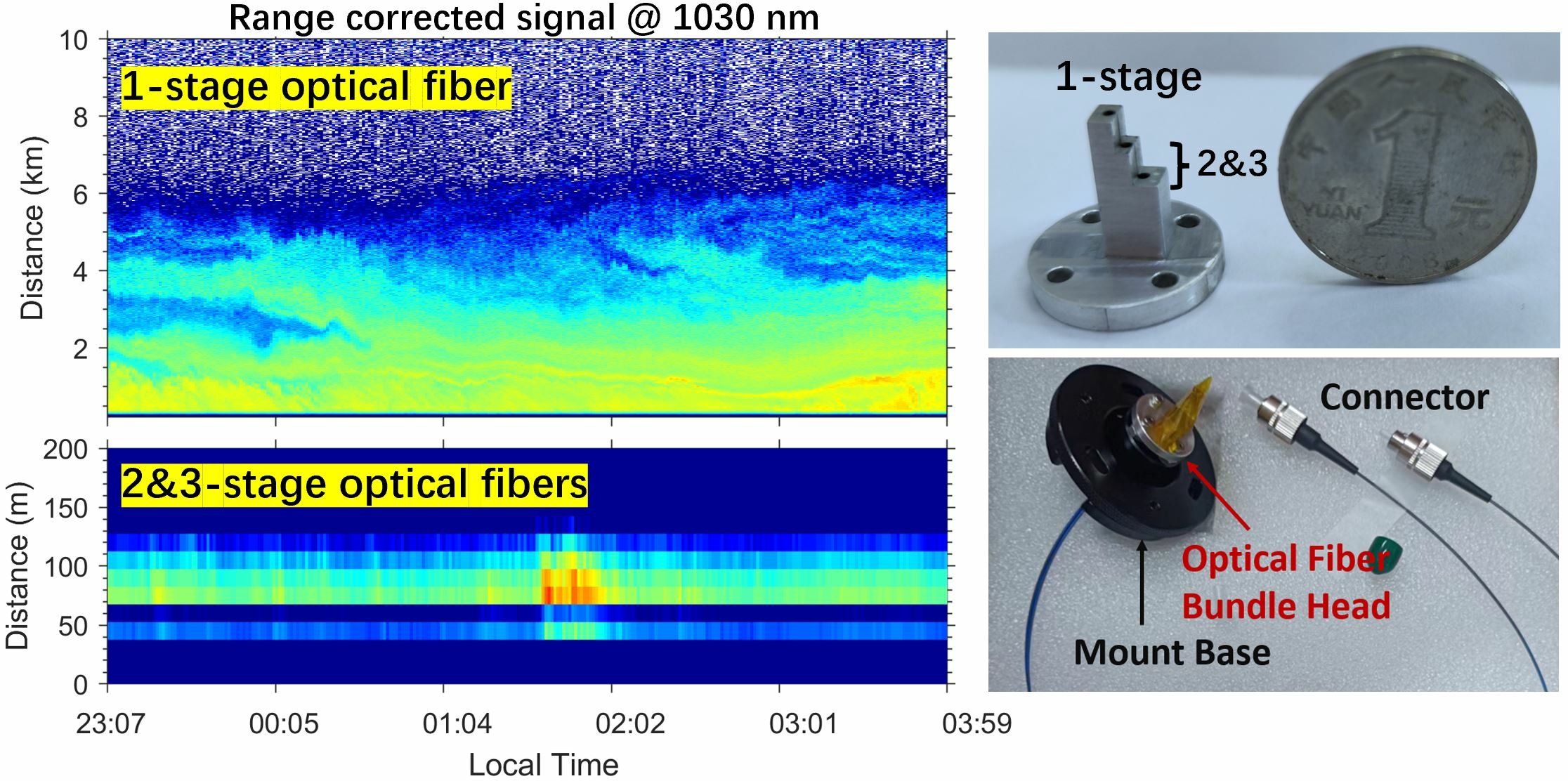
2.1. Imaging of Laser Beam by Receiving Telescope in a Biaxial Lidar System

For a biaxial lidar system, the axis of transmitting the laser beam has a certain distance from the optical axis of receiving the telescope, as shown in Figure 1. Laser beams at different range levels are imaged by the telescope and focused on different image planes. For a laser beam from far range, which is at a distance of around 10 km, it is focused on the center at the focal plane of the telescope. For a laser beam at near-range, which is at a distance of <500 m, it is imaged behind the focal plane at a certain distance from the optical axis of the telescope. While the laser beam has mid-range scattering volume, it is focused in between. Images of laser beams from different range levels can be traced and are illustrated in Figure 1. In a conventional biaxial lidar system, a small circle diaphragm was placed at the center of the focal plane, which would receive all backscatter light from far-range; however, it would block partial or all backscatter light from near-range scattering volume, depending on the radius of the diaphragm, which would lead to the transition zone or blind zone in the lidar signal. The radius of the diaphragm needs to be optimized between near-range detection efficiency and solar background suppression. Usually, this radius is on the order of 1 mm for a focal length of 1000 mm or so. In order to improve the efficiency of light receiving at near-range while maintaining sufficient solar background suppression, additional diaphragms need to be inserted at the focusing positions of laser beams from mid- and near-range distances.

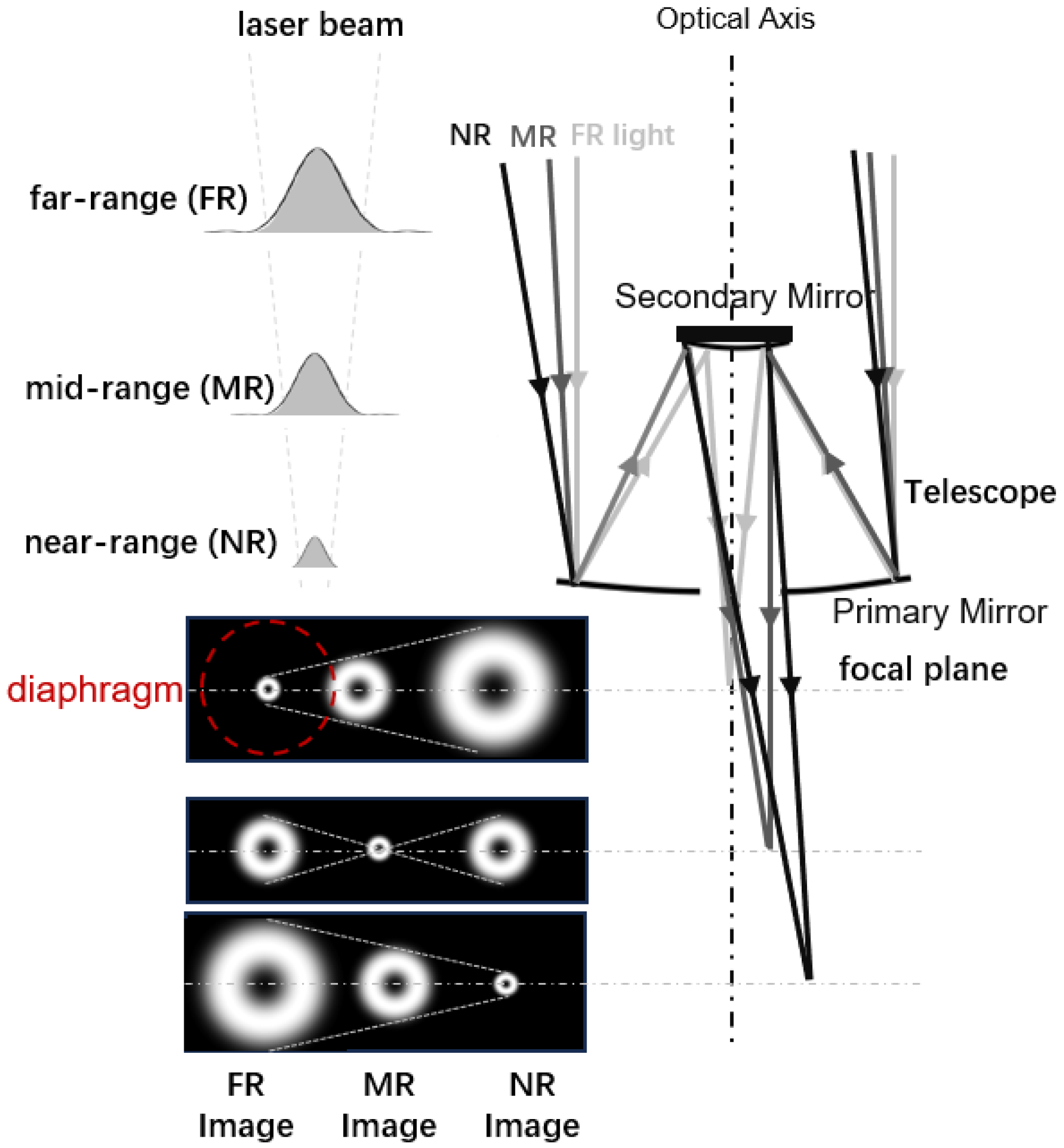
2.2. Optical Fiber Bundle Design

Optical fibers can be used as diaphragms and have better capacity for light transformation. In order to improve near-range light-collecting efficiency, several optical fibers can be placed at the focusing positions of laser beams from different range levels. In Figure 2, an example of this optical fiber bundle head with seven stages is displayed, targeting the scattering volume from 40 m to 15 km. Each stage is a few millimeters high, depending on the specific systematic parameters of the focal length of the receiving telescope and the distance between the transmitting laser beam and the optical axis of the telescope. Each optical fiber goes through the optical fiber bundle head and can be bundled after leaving the optical fiber bundle head, as is shown in Figure 2b. The optical fiber planted at the center of the optical fiber bundle aims at far-range signal detection, while the other six optical fibers are responsible for mid-range and near-range signal detection and can be bundled together.
The final GOF of this optical fiber bundle can be determined according to the physical model proposed by Harms (1978), assuming the distance between the transmitting laser beam and the optical axis of the receiving telescope ( d ) of 500 mm, the focal length of the telescope ( f ) of 500 mm, the optical fiber N/A of 0.22, and the diameter of the optical fiber of 200 μm. The FOV of each optical fiber is 0.4 mrad. The detailed parameters of the seven-stage optical fiber head are listed in Table 1. It would lead to a binding zone of 350 m and a transitioning zone from 350 to 900 m if only one optical fiber is installed at the center of the optical fiber bundle head, as shown in Figure 3. All the other six optical fibers cover a detection range of a few tens of meters, between 40 and 400 m. Thus, bundling the seven optical fibers can reach the detection of backscatter light starting at 40 m.

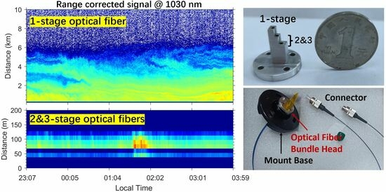
2.3. Low Blind Zone Lidar at 1030 nm

In order to verify the performance of the design described above, an elastic lidar at 1030 nm was built with a three-stage optical fiber bundle. This lidar aims at aerosol detection from 50 m to 10 km. A 1030 nm micro-pulse laser is used with a repetition rate of 5 kHz and a single pulse energy of 160 μJ. A 136-millimeter Ritchey-Chretien telescope with a focal length of 500 mm is used for backscatter light detection. Si-APD is used for light detection, with an effective signal dynamic range of four orders of magnitude. The detailed parameters of this lidar system can be found in Table 2. To meet the requirement of the seven-order dynamic range of a near-infrared lidar signal from 50 m to 10 km, two detection channels are designed to receive far- and near-range light from the central optical fiber and the other optical fibers, respectively. Narrow interference filters (NIFs) with a central wavelength of 1030 nm and FWHM of 3 nm are used to block solar background. In order to eliminate the angular response effects of NIFs, achromatic fiber collimators are used to form a collimated light beam. The collimated beam goes through neutral-density filters and NIFs. Ultimately, the light beam is coupled into the Si-APD by the other chromatic fiber collimator, as can be seen in Figure 4.
The design of the optical fiber bundle head is optimized based on the listed systematic parameters in Table 2. Scattering volumes at 50, 100, and 5000 m are selected as the optimized objects for the highest detection efficiency. The first two ranges stand for the objective for the near-range channel, while the target located at 5000 m stands for the objective for the far-range channel (Figure 5a). The images of the scattering volume from the three different ranges are ray-traced by ZEMAX [32]. The minimum imaging spots are displayed in Figure 5a. The scattering volume at 5000 m is projected at the center of the focal plane, 2 mm above the bottom of the primary mirror. The size of the imaging spot is around 50 μm, which can be fully received by the optical fiber with an effective core size of 200 μm in the first stage, considering the effective core size of 200 μm. The scattering volume at 100 m is projected on the plane with 0.45 mm below the primary mirror and around 1 mm at the right of the optical axis, and its size is 220 μm. While scattering volume at 50 m, it is projected on the plane with 2.98 mm behind the primary mirror and a spot size of 280 μm. Although only 80% of near-range backscatter scattering light can be collected by the optical fibers, it is still too strong for the Si-APD detector. Therefore, additional attenuation is still needed for the near-range channel. According to the ray-tracing results, a three-stage optical fiber head was designed with holes of 1 mm at the center of each stage. The overall size of this optical fiber head is comparable to a 1-yuan coin, as shown in Figure 5b. Three optical fibers were then inserted into the holes of each stage and fastened with glue. The optical fiber from the highest stage is covered by an opaque plastic tube to avoid contamination from the ambient light, and an FC connector is installed on the other side of the optical fiber to be connected to the fiber collimator, as is displayed in Figure 5c. The other two optical fibers are bundled, and the same connector is installed.
The optical fiber bundle is installed in the 1030 nm elastic lidar system. The general mechanical design of this lidar system is shown in Figure 6. It can be noted that the optical fiber head is installed at the exit pupil of the telescope (Figure 6b). This lidar system was developed and then tested with experiments.

3. Results

A prototype of this 1030 nm elastic lidar with low blind zone capability was built in the laboratory. An experiment to verify the detection performance was conducted on the campus of Wuhan University on 4 August 2023. The measurement site is at the city center of Wuhan, which is a megacity with a population of more than 10 million. The lidar system was tilted with an elevation angle of 17° (73° off zenith). Horizontal measurements of near-surface aerosols with homogeneous distributions cannot be conducted due to the obstructions of high buildings surrounding them. After the position of the optical fiber bundle head was adjusted manually to obtain the largest far- and near-range signal, the lidar system stayed in observation mode. Time-series profiles of the range-corrected signal from the far-range detection channel are displayed in Figure 7a. The complex evolution of aerosols within the atmospheric planetary boundary layer can be noticed. Aerosols within 5 km (in distance) can be easily distinguished and are relatively continuous in time. Aerosols near the surface are expected to be emitted by point sources and influenced by city buildings after low-level transport. As evidence, the range-corrected signal at 80–100 m has strong indications of point sources, as several small-scale enhancements of the backscatter signal can be identified. This feature can be noticed at near-range channel signals, especially between 01:30 and 02:00 a.m., when a burst of near-surface aerosol plume could be noticed (see Figure 7b). In addition, the burst of near-surface aerosol loading can be corroborated by near-surface visibility measurements, which can be seen in Figure 7c. Based on these test measurement results, we could confirm that the far-range channel can provide a broader picture of aerosols and clouds, while the near-range channel can provide information about aerosols near the surface. These features and information can be merged to diagnose aerosol vertical and horizontal transport, especially the upward flux of aerosols from point sources or from the earth’s surface.
A typical signal profile after background and deadtime correction is shown in Figure 8a. The photon counting rate of the far-range signal was adjusted to be less than 10 MHz, which is in the linear response range of the Si-APD. The near-range signal peak value is adjusted to be comparable to the maximum value of the far-range signal, which was achieved by adding a neutral density filter of OD = 0.5 and weakening the coupling efficiency of the near-range fiber coupler. Near-range signals have double peaks at 45 and 100 m, respectively, which agrees with simulations for this three-stage optical fiber bundle. The signal quickly decreases as the range bin increases. Nevertheless, the near-range channel can cover signal detection from 45 to 120 m, which is sensitive to low-level aerosol layers and aerosol vertical transport. Signal after range correction is provided in Figure 8b and can reveal the receiving efficiency of different channels. According to the shape of the range-corrected signal from the far-range channel, the starting range with complete overlap is more than 400 m. A near-range detection channel can produce an effective and useful signal at 50 m. The maximum detection range can exceed 10 km after half-hour signal averaging, according to the signal-to-noise ratio plot in Figure 9. This is sufficient to capture the most aerosol loadings within the troposphere and is a good support for the far-range detection capability of using an optical fiber bundle for backscatter light receiving.

4. Discussion

In this research, a new method based on an optical fiber bundle was introduced for atmospheric lidars. The optical fiber bundle head with multiple stages was optimized according to the imaging of laser beams at different range levels. A 1030 elastic lidar equipped with this optical fiber bundle was developed. Consistency experiment results with simulations were obtained and indicate an effective lowest detection distance down to 50 m and a maximum detection range of 10 km.
The overall performance of the optical fiber bundle is closely associated with the number of stages and optical fibers. The lidar prototype with a three-stage optical fiber bundle still has a blind zone at 200–350 m. Adding more stages and optical fibers can increase the full-range detection efficiency, according to our simulation (see Figure 3). However, considering the size of optical fiber and the precision of mechanical fabrication, the number of stages cannot be infinite. According to our experience, the maximum number of stages is 4, based on the 1030 nm lidar system parameters. However, if thinner optical fiber can be used, for instance, 100 or 150 μm, more stages can be fabricated on top of the optical fiber head. More importantly, if the focus size of the receiving telescope can be decreased, optical fibers with a core size less than 100 μm can also be considered. A good example is the Cloud Thickness from Offbeam Lidar Returns (THOR) [35]. In the THOR lidar system, an optical fiber bundle consisting of 250,000 optical fibers with a core size of 50 μm was fabricated and used for receiving multiple scatterings of light from dense water clouds [35].
For the determination of vertical aerosol distribution, the final geometrical overlap factor needs to be corrected, which can be performed by horizontal experiments [36].
It should be noted that the near- and far-range channels can be bundled together, and a fiber optic attenuator can be used to avoid saturation of the near-range signal. Based on this approach, only one detector would be sufficient so that it could increase system robustness and reduce system complexity.

5. Conclusions

In this research, an attempt at a light-receiving scheme is proposed for atmospheric lidar based on an optical fiber bundle. The principle of geometrical overlap factor for a biaxial lidar system is analyzed. The design of a multiple-stage optical fiber head aimed at near- and far-range signal detection is introduced. A three-stage optical fiber bundle was fabricated and demonstrated on a 1030 nm elastic lidar. Experiment results suggest effective signal detection down to 50 m and a maximum detection range of 10 km, which are consistent with simulations.
This optical fiber bundle can be easily applied in other biaxial systems, for instance, a biaxial Doppler wind lidar, to improve the near-range detection performance [37]. It should be noted that this scenario can also be used in Raman lidar systems as well, because the divergence of near-range backscatter light can be transformed by using a dichromatic fiber coupler. This approach is useful for water vapor and temperature measurement and would bring new possibilities to the investigation of atmosphere-land interactions.

Author Contributions

All the authors made contributions to this research and manuscript. This research was conceived by Z.Y., X.W. and Y.Y. The lidar system was built by Z.Y. and L.W. The field experiments were conducted by Z.Y. and Q.C. The data was analyzed by Z.Y. with contributions from Q.C.; The manuscript was written by Z.Y. All authors have joined the scientific discussion, manuscript review, and editing. All authors have read and agreed to the published version of the manuscript.

Funding

This work was supported by the National Natural Science Foundation of China (grant Nos. 42205130, 62275202, and 62105248), the National Key Research and Development Program of China (grant No. 2021YFC3090200), and the Innovation and Development Project of China Meteorological Administration (grant No. CXFZ2022J060).

Data Availability Statement

The datasets generated during and/or analyzed during the current study are available from the corresponding author upon reasonable request.

Acknowledgments

We are grateful to Hengzhi Wang and Lei Zhao for their technical help in lidar development. We are grateful to Song Mao and Xiangyu Dong for their help in field experiments. It was not possible to perform this research without their assistance.

Conflicts of Interest

The authors declare no conflict of interest.

References

  1. Li, Z.; Guo, J.; Ding, A.; Liao, H.; Liu, J.; Sun, Y.; Wang, T.; Xue, H.; Zhang, H.; Zhu, B. Aerosol and boundary-layer interactions and impact on air quality. Natl. Sci. Rev. 2017, 4, 810–833. [Google Scholar] [CrossRef]
  2. Li, Z.; Wang, Y.; Guo, J.; Zhao, C.; Cribb, M.C.; Dong, X.; Fan, J.; Gong, D.; Huang, J.; Jiang, M.; et al. East Asian Study of Tropospheric Aerosols and their Impact on Regional Clouds, Precipitation, and Climate (EAST-AIRCPC). J. Geophys. Res. Atmos. 2019, 124, 13026–13054. [Google Scholar] [CrossRef]
  3. Wulfmeyer, V.; Hardesty, R.M.; Turner, D.D.; Behrendt, A.; Cadeddu, M.P.; Di Girolamo, P.; Schlüssel, P.; Van Baelen, J.; Zus, F. A review of the remote sensing of lower tropospheric thermodynamic profiles and its indispensable role for the understanding and the simulation of water and energy cycles. Rev. Geophys. 2015, 53, 819–895. [Google Scholar] [CrossRef]
  4. He, Y.; Yi, F.; Liu, F.; Yin, Z.; Zhou, J. Ice Nucleation of Cirrus Clouds Related to the Transported Dust Layer Observed by Ground-Based Lidars over Wuhan, China. Adv. Atmos. Sci. 2022, 39, 2071–2086. [Google Scholar] [CrossRef]
  5. He, Y.; Yin, Z.; Liu, F.; Yi, F. Technical note: Identification of two ice-nucleating regimes for dust-related cirrus clouds based on the relationship between number concentrations of ice-nucleating particles and ice crystals. Atmos. Chem. Phys. 2022, 22, 13067–13085. [Google Scholar] [CrossRef]
  6. Yin, Z.; Yi, F.; He, Y.; Liu, F.; Yu, C.; Zhang, Y.; Wang, W. Asian dust impacts on heterogeneous ice formation at Wuhan based on polarization lidar measurements. Atmos. Environ. 2021, 246, 118166. [Google Scholar] [CrossRef]
  7. Brooks, I.M. Finding boundary layer top: Application of a wavelet covariance transform to lidar backscatter profiles. J. Atmos. Ocean. Technol. 2003, 20, 1092–1105. [Google Scholar] [CrossRef]
  8. Pal, S. Monitoring Depth of Shallow Atmospheric Boundary Layer to Complement LiDAR Measurements Affected by Partial Overlap. Remote Sens. 2014, 6, 8468–8493. [Google Scholar] [CrossRef]
  9. Pal, S.; Lopez, M.; Schmidt, M.; Ramonet, M.; Gibert, F.; Xueref-Remy, I.; Ciais, P. Investigation of the atmospheric boundary layer depth variability and its impact on the 222Rn concentration at a rural site in France. J. Geophys. Res. Atmos. 2015, 120, 623–643. [Google Scholar] [CrossRef]
  10. Lange, D.; Behrendt, A.; Wulfmeyer, V. Compact Operational Tropospheric Water Vapor and Temperature Raman Lidar with Turbulence Resolution. Geophys. Res. Lett. 2019, 46, 14844–14853. [Google Scholar] [CrossRef]
  11. Wang, L.; Yin, Z.; Bu, Z.; Wang, A.; Mao, S.; Yi, Y.; Müller, D.; Chen, Y.; Wang, X. Quality assessment of aerosol lidars at 1064 nm in the framework of the MEMO campaign. Atmos. Meas. Tech. Discuss. 2023, 2023, 1–18. [Google Scholar] [CrossRef]
  12. Wandinger, U. Introduction to Lidar. In Lidar: Range-Resolved Optical Remote Sensing of the Atmosphere; Weitkamp, C., Ed.; Springer: New York, NY, USA, 2005; pp. 1–18. [Google Scholar]
  13. Wiegner, M.; Madonna, F.; Binietoglou, I.; Forkel, R.; Gasteiger, J.; Geiß, A.; Pappalardo, G.; Schäfer, K.; Thomas, W. What is the benefit of ceilometers for aerosol remote sensing? An answer from EARLINET. Atmos. Meas. Tech. 2014, 7, 1979–1997. [Google Scholar] [CrossRef]
  14. Wiegner, M.; Geiß, A. Aerosol profiling with the Jenoptik ceilometer CHM15kx. Atmos. Meas. Tech. 2012, 5, 1953–1964. [Google Scholar] [CrossRef]
  15. Sassen, K. Polarization in Lidar. In Lidar: Range-Resolved Optical Remote Sensing of the Atmosphere; Weitkamp, C., Ed.; Springer: New York, NY, USA, 2005; pp. 19–42. [Google Scholar]
  16. Chen, Q.; Mao, S.; Yin, Z.; Yi, Y.; Li, X.; Wang, A.; Wang, X. Compact and efficient 1064 nm up-conversion atmospheric lidar. Optics Express 2023, 31, 23931–23943. [Google Scholar] [CrossRef]
  17. Wandinger, U.; Ansmann, A. Experimental determination of the lidar overlap profile with Raman lidar. Appl. Opt. 2002, 41, 511–514. [Google Scholar] [CrossRef] [PubMed]
  18. Gong, W.; Mao, F.; Li, J. OFLID: Simple method of overlap factor calculation with laser intensity distribution for biaxial lidar. Opt. Commun. 2011, 284, 2966–2971. [Google Scholar] [CrossRef]
  19. Harms, J.; Lahmann, W.; Weitkamp, C. Geometrical compression of lidar return signals. Appl. Opt. 1978, 17, 1131–1135. [Google Scholar] [CrossRef]
  20. Stelmaszczyk, K.; Dell’Aglio, M.; Chudzyński, S.; Stacewicz, T.; Wöste, L. Analytical function for lidar geometrical compression form-factor calculations. Appl. Opt. 2005, 44, 1323–1331. [Google Scholar] [CrossRef]
  21. Mao, F.; Gong, W.; Li, J. Geometrical form factor calculation using Monte Carlo integration for lidar. Opt. Laser Technol. 2012, 44, 907–912. [Google Scholar] [CrossRef]
  22. Engelmann, R.; Kanitz, T.; Baars, H.; Heese, B.; Althausen, D.; Skupin, A.; Wandinger, U.; Komppula, M.; Stachlewska, I.S.; Amiridis, V.; et al. The automated multiwavelength Raman polarization and water-vapor lidar PollyXT: The neXT generation. Atmos. Meas. Tech. 2016, 9, 1767–1784. [Google Scholar] [CrossRef]
  23. Balin, Y.S.; Bairashin, G.S.; Kokhanenko, G.P.; Penner, I.E.; Samoilova, S.V. LOSA-M2 aerosol Raman lidar. Quantum Electron. 2011, 41, 945. [Google Scholar] [CrossRef]
  24. Wang, J.; Liu, W.; Liu, C.; Zhang, T.; Liu, J.; Chen, Z.; Xiang, Y.; Meng, X. The Determination of Aerosol Distribution by a No-Blind-Zone Scanning Lidar. Remote Sens. 2020, 12, 626. [Google Scholar] [CrossRef]
  25. Comeron, A.; Sicard, M.; Kumar, D.; Rocadenbosch, F. Use of a field lens for improving the overlap function of a lidar system employing an optical fiber in the receiver assembly. Appl. Opt. 2011, 50, 5538–5544. [Google Scholar] [CrossRef]
  26. Campbell, J.R.; Hlavka, D.L.; Welton, E.J.; Flynn, C.J.; Turner, D.D.; Spinhirne, J.D.; Scott, V.S., III; Hwang, I. Full-time, eye-safe cloud and aerosol lidar observation at atmospheric radiation measurement program sites: Instruments and data processing. J. Atmos. Ocean. Technol. 2002, 19, 431–442. [Google Scholar] [CrossRef]
  27. Gaixia, Z.; Yinchao, Z.; Zongming, T.; Xiaoqin, L.; Shisheng, S.; Kun, T.; Yonghui, L.; Jun, Z.; Huanling, H. Lidar geometric form factor and its effect on aerosol detection. Chin. J. Quantum Electron. 2005, 2, 6. [Google Scholar]
  28. Newsom, R.K.; Turner, D.D.; Mielke, B.; Clayton, M.; Ferrare, R.; Sivaraman, C. Simultaneous analog and photon counting detection for Raman lidar. Appl. Opt. 2009, 48, 3903–3914. [Google Scholar] [CrossRef] [PubMed]
  29. Wang, L.; Yin, Z.; Zhao, B.; Mao, S.; Zhang, Q.; Yi, Y.; Wang, X. Performance of Wide Dynamic Photomultiplier Applied in a Low Blind Zone Lidar. Remote Sens. 2023, 15, 4404. [Google Scholar] [CrossRef]
  30. Agishev, R.R.; Comeron, A. Spatial filtering efficiency of monostatic biaxial lidar: Analysis and applications. Appl. Opt. 2002, 41, 7516–7521. [Google Scholar] [CrossRef]
  31. Freudenthaler, V. Optimized background suppression in near field lidar telescopes. In Proceedings of the 6th ISTP International Symposium on Tropospheric Profiling: Needs and Technologies, Leipzig, Germany, 14–20 September 2003. [Google Scholar]
  32. Kokkalis, P. Using paraxial approximation to describe the optical setup of a typical EARLINET lidar system. Atmos. Meas. Tech. 2017, 10, 3103–3115. [Google Scholar] [CrossRef]
  33. Mei, L.; Brydegaard, M. Atmospheric aerosol monitoring by an elastic Scheimpflug lidar system. Opt. Express 2015, 23, A1613–A1628. [Google Scholar] [CrossRef]
  34. Xian, J.; Sun, D.; Amoruso, S.; Xu, W.; Wang, X. Parameter optimization of a visibility LiDAR for sea-fog early warnings. Opt. Express 2020, 28, 23829–23845. [Google Scholar] [CrossRef]
  35. Cahalan, R.F.; McGill, M.; Kolasinski, J.; Várnai, T.; Yetzer, K. THOR—Cloud Thickness from Offbeam Lidar Returns. J. Atmos. Ocean. Technol. 2005, 22, 605–627. [Google Scholar] [CrossRef]
  36. Vande Hey, J.; Coupland, J.; Foo, M.H.; Richards, J.; Sandford, A. Determination of overlap in lidar systems. Appl. Opt. 2011, 50, 5791–5797. [Google Scholar] [CrossRef] [PubMed]
  37. Li, Y.; Wang, C.; Xue, X.; Wang, Y.; Shang, X.; Jia, M.; Chen, T. Study on the Parameters of Ice Clouds Based on 1.5 µm Micropulse Polarization Lidar. Remote Sens. 2022, 14, 5162. [Google Scholar] [CrossRef]
Figure 1. Optical scheme of biaxial lidar for near-range (NR), mid-range (MR), and far-range (FR) imaging. Images of laser beams at different imaging planes with certain distances to the telescope are shown at the lower left part, while the laser beam is projected to a doughnut-shaped circle due to the central obstruction of the secondary mirror.
Remotesensing 15 04643 g001
Figure 2. The optical fiber bundle head consists of seven stages. (a) Front view of the optical fiber bundle head. (b) Vertical view. At the center of each stage, an optical fiber is planted. The optical fibers go through the optical fiber bundle head and can be bundled after leaving the optical fiber bundle head.
Remotesensing 15 04643 g002
Figure 3. Theoretical geometrical overlap factor for a biaxial lidar with a seven-stage optical fiber bundle. A zoom-in plot of the geometrical overlap factor between 0 and 150 m is attached in the middle.
Remotesensing 15 04643 g003
Figure 4. Design of a 1030 nm elastic lidar system, including the key component of a three-stage optical fiber bundle. OFBH is the optical fiber bundle head. FC stands for dichromatic fiber collimator. NDF stands for neutral density filter. NIF is the narrowband interference filter. NR and FR stand for near-range and far-range, respectively.
Remotesensing 15 04643 g004
Figure 5. (a) Design of a three-stage optical fiber head. Shot lines with colors represent the focusing positions of scattering volume from different distances. The width of the shot lines represents the size of the imaging spots. The x-axis stands for the distance of images to the optical axis of the receiving telescope, while the y-axis stands for the vertical distance of images to the focal plane. (b) Photo of the optical fiber bundle head in comparison with a 1-yuan coin; (c) Photo of the optical fiber bundle while a metal mount base is installed for adjustment.
Remotesensing 15 04643 g005
Figure 6. The mechanical design of the 1030 nm elastic lidar has a size of 654 (length) × 554 (width) × 371 (height) mm. (a) Front view of the lidar; (b) back view of the lidar. 1 is the telescope; 2 is the Si-APDs; 3 is the control PC; 4 is the power module; 5 is the fiber couplers; 6 is the optic module; 7 is the laser head; 8 is the optical fiber bundle head installed on a mounting base; 9 is the control board with digitizer installed; (c) A back-view photo of the lidar system.
Remotesensing 15 04643 g006
Figure 7. Time-distance plot of the range-corrected signal from the 1030 nm elastic lidar and time series of visibility from a ground-based visibility sensor. (a) Logarithm of range-corrected signal (in the unit of 1000 * photon count * km2) from the far-range channel. (b) Logarithm of range-corrected signal (in the unit of 1000 * photon count * km2) from the near-range channel. (c) Visibility at ground level. The spatiotemporal resolution is 15 m and 1 min for the lidar signal.
Remotesensing 15 04643 g007
Figure 8. Elastic lidar signal at 1030 nm. (a) Near- and far-range signals; (b) range-corrected signals.
Remotesensing 15 04643 g008
Figure 9. Signal-to-Noise Ratio (SNR) of far-range channel signal (a) and near-range channel signal (b). The minimum threshold for maximum detection range is marked by a red dash line. The maximum detection range is 10.06 km, assuming a minimum threshold of SNR = 3 [34].
Remotesensing 15 04643 g009
Table 1. Parameters of the optical fiber heads with seven stages and three stages, assuming the distance between the transmitting laser beam and the optical axis of the receiving telescope ( d ) of 200 mm, the focal length of the telescope ( f ) of 500 mm, the optical fiber N/A of 0.22, and the diameter of the optical fiber of 150 μm for the seven-stage optical fiber head and 200 μm for the three-stage optical fiber head.
Seven-Stage Optical Fiber Head
Stage NumberDistance to the Optical Axis (mm)Distance to the Base (mm)
1022.00
20.3421.17
30.6820.34
41.0219.51
51.3618.68
61.7017.85
72.0417.02
Three-stage optical fiber head
Stage NumberDistance to the optical axis (mm)Distance to the base (mm)
1022.00
21.0119.55
32.0617.02
Table 2. Parameters of the 1030 nm elastic lidar, where d stands for the distance between the laser beam and the optical axis of the receiving telescope and NIF stands for narrowband interference filter.
ItemParameters
Laser5 kHz and 160 μJ
Telescopefocal length: 500 mm
divergence: 0.2 mrad
diameter of the primary mirror: 136 mm
focus size: ≤30 μm
Optical fibercore size: 200 μm
d200 mm
NIF1030 ± 3 nm
Fiber collimatorfocal length of 40 mm and FC/PC connector
Disclaimer/Publisher’s Note: The statements, opinions and data contained in all publications are solely those of the individual author(s) and contributor(s) and not of MDPI and/or the editor(s). MDPI and/or the editor(s) disclaim responsibility for any injury to people or property resulting from any ideas, methods, instructions or products referred to in the content.

