Estimation of Daily Seamless PM_2.5 Concentrations with Climate Feature in Hubei Province, China

Abstract

The urgent necessity for precise and uninterrupted PM_2.5 datasets of high spatial–temporal resolution is underscored by the significant influence of PM_2.5 on weather, climate, and human health. This study leverages the AOD reconstruction method to compensate for missing values in the MAIAC AOD throughout Hubei Province. The reconstructed AOD dataset, exhibiting an R²/RMSE of 0.76/0.18, compared to AERONET AOD, was subsequently used for PM_2.5 estimation. Our research breaks from traditional methodologies that solely depend on latitude and longitude information. Instead, it emphasizes the use of climate feature as an input for estimating PM_2.5 concentrations. This strategic approach prevents potential spatial discontinuities triggered by geolocation information (latitude and longitude), thus ensuring the precision of the PM_2.5 estimation (sample/spatial CV R² = 0.91/0.88). Moreover, we proposed a method for identifying the absolute feature importance of machine-learning models. Contrasted with the relative feature-importance property typical of machine-learning models (a minor difference in the order of top three between geolocation-based and climate-feature-based models, and the slight difference in the top three: 0.08%/0.17%), our method provides a more comprehensive explanation of the absolute significance of features to the model (maintaining the same order and a larger difference in the top three: 0.99%/0.72%). Crucially, our findings demonstrated that AOD reconstruction can mitigate the overestimation of annual mean PM_2.5 concentrations (ranging from 0.52 to 9.28 µg/m³). In addition, the seamless PM_2.5 dataset contributes to reducing the bias in exposure risk assessment (ranging from −0.11 to 9.81 µg/m³).

1. Introduction

Air pollution, chiefly from PM_2.5 (particulate matter with a diameter of 2.5 microns or less), presents a significant health hazard [1], causing respiratory illnesses [2], cardiovascular complications [3], and even premature mortality [4]. Various methods, ranging from ground-based monitoring stations [5] to numerical simulations [6] and satellite remote sensing [7], have been utilized over recent decades to collect PM_2.5 data. Ground-based stations, while precise, are spatially sparse and unevenly distributed. Prior research typically combined spatial interpolation methods such as Kriging [8] and inverse distance weighted [9] with station observations to develop spatiotemporally continuous PM_2.5 datasets, albeit with restricted accuracy. Numerical simulations leverage algorithms to mimic atmospheric processes and predict spatial–temporal PM_2.5 concentrations, with accuracy heavily dependent on emissions inventory, meteorological input data, and parameterization of chemical and physical processes [10].

Over the past decade, satellite remote sensing has gained prominence as a potent tool for capturing aerosol optical depth (AOD), a parameter closely related to surface PM_2.5 levels. Satellite-derived AOD possesses several advantages, including extensive spatial coverage, repeated observations, and global data availability [11]. Moreover, the application of machine-learning techniques to estimate PM_2.5 concentrations from satellite AOD measurements has gained traction [12], leveraging the correlation between AOD and ground-based PM_2.5 observations to facilitate estimations in regions lacking ground-based monitoring stations. However, the utility of satellite AOD is curtailed by weather conditions such as cloud cover and rain, resulting in spatial gaps in AOD and PM_2.5 datasets [13]. In response, researchers have proposed an AOD reconstruction method to create a comprehensive AOD dataset, which has proven beneficial for PM_2.5 estimation [14]. Yet, the conventional practice of using latitude and longitude as input features leads to spatial discontinuities in the resultant PM_2.5 dataset [15,16,17]. This inconsistency arises due to longitude and latitude being referenced to two straight lines of zero degrees rather than a two-dimensional spatial plane. Meanwhile, existing studies interpreting feature contributions typically employ the relative feature-importance attribute [18,19], neglecting the interplay between input features and, thereby, resulting in an inaccurate interpretation of feature significance in the estimation model [20].

To mitigate the issues outlined above, this study proposes a novel approach that substitutes climate feature for latitude and longitude information to describe spatial characteristics, thus creating a more accurate PM_2.5 estimation model. Additionally, a random rearrangement method will be used to calculate absolute feature importance. Our study primarily focuses on Hubei province in China, covering the period from 2015 to 2020. The initial stage involves filling the gaps in the satellite AOD dataset, which are caused by factors such as cloud cover and rain. Following this, machine-learning algorithms will be deployed to estimate daily average PM_2.5 concentrations. Furthermore, we will evaluate the significance of AOD reconstruction for PM_2.5 exposure risk.

2. Materials and Methods

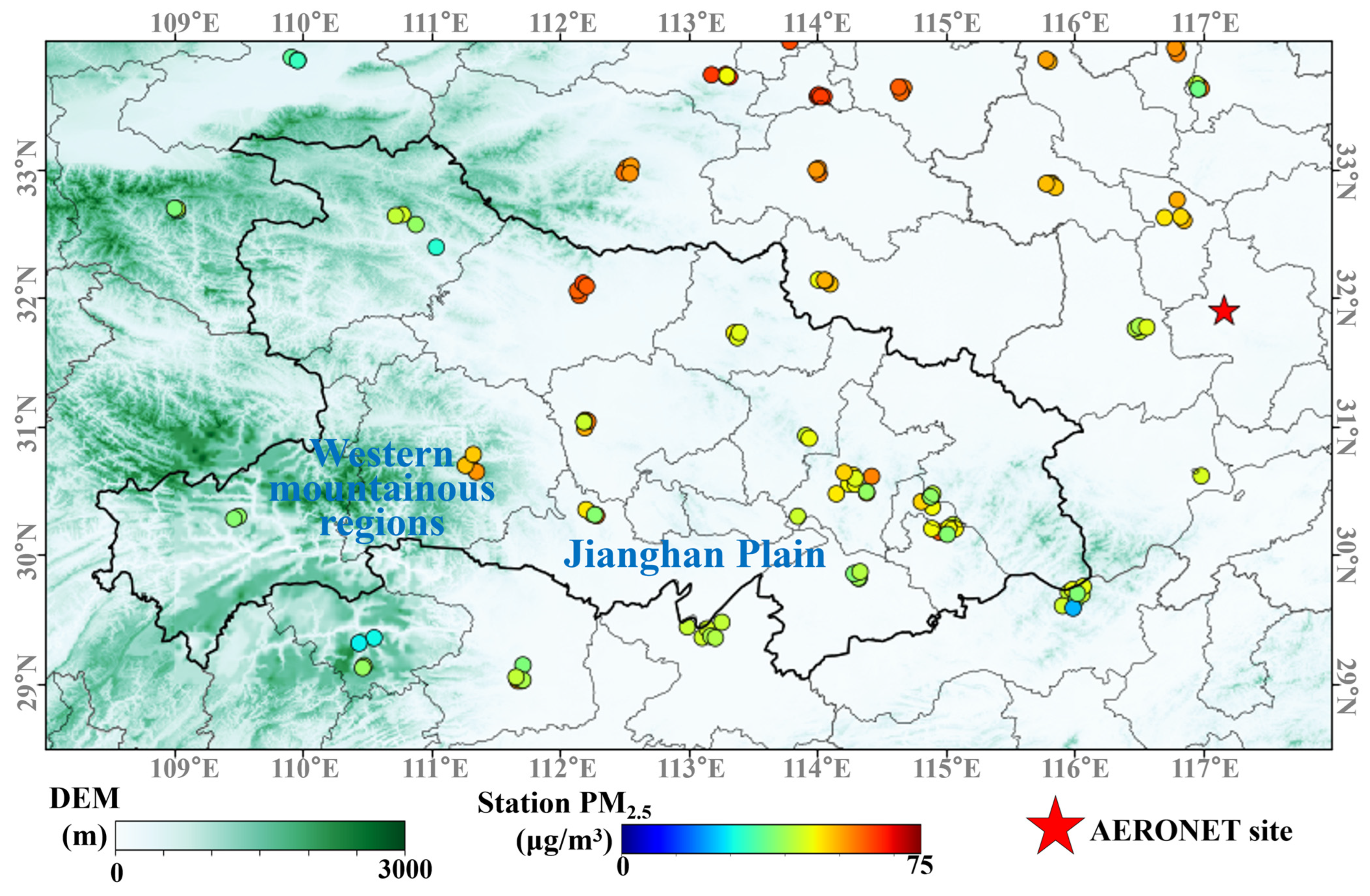
2.1. Study Region

Hubei Province, nestled in the heart of China, is defined by its richly varied topography. As depicted in Figure 1, the province, with openings to the south, is flanked by mountain ranges to the west, north, and east, creating a unique geographical pattern. This unique positioning places Hubei Province within the influence of four haze pollution zones: the North China Plain, Yangtze River Delta, Pearl River Delta, and Sichuan Basin [21]. This makes the province notably vulnerable to the ingress of external air pollutants, which can significantly exacerbate the already substantial pollution levels. Moreover, the accelerated growth and development of heavy industries—notably the automobile, machinery, and steel sectors—have further strained the local air quality [22]. This dual pressure from both external influxes and local industrial expansion creates a challenging scenario for air-quality management in Hubei Province.

2.2. Datasets

2.2.1. PM_2.5 Station Data

This study employs data from 136 PM_2.5 monitoring stations acquired from the China National Environmental Monitoring Centre (CEMC, http://www.cnemc.cn/, accessed on 25 July 2023). The annual average PM_2.5 levels at each station are visually represented in Figure 1, with Xiangyang recording the highest value, closely followed by Jingmen. To generate a daily estimation of PM_2.5 levels, hourly readings from 2015 to 2020 were compiled into daily averages. This was done under the condition that only the data with an effective duration exceeding 16 h per day were incorporated. Consequently, a comprehensive set of 261,586 ground PM_2.5 records pertaining to the study area in Hubei Province was compiled for further PM_2.5 analysis.

2.2.2. AOD Data

The Multiangle Implementation of Atmospheric Correction (MAIAC) Aerosol Optical Depth (AOD) products, furnished with a spatial resolution of 1 km × 1 km, are developed using data from NASA’s MODIS TERRA satellite, which collects data at 10:30 a.m. local time, and the AQUA satellite, operating at 1:30 p.m. local time [23]. This study utilizes the MAIAC AOD products at 550 nm for Hubei Province, spanning a period of six years from 1 January 2015 through 31 December 2020, sourced from the Google Earth Engine (https://code.earthengine.google.com, accessed on 25 July 2023). However, the accuracy of satellite AOD can be compromised due to atmospheric conditions, such as cloud cover or precipitation [13], resulting in spatiotemporal gaps in the MAIAC AOD data. As illustrated in Figure 2, the year 2017 had the highest annual effective observation rate of the MAIAC AOD, being approximately 4% higher than the other years.

To fill in these data gaps in MAIAC AOD, this study applies the Modern Era Retrospective analysis for Research and Applications, Version 2 (MERRA2) dataset. In particular, we use the 550 nm AOD measurements, having a spatial resolution of 0.625° × 0.5° [24], obtained from the Goddard Earth Sciences Data and Information Services Center (GES DISC) at NASA’s Goddard Space Flight Center (https://gmao.gsfc.nasa.gov/reanalysis/MERRA-2, accessed on 25 July 2023). To facilitate the AOD reconstruction process, these hourly AOD values were translated into daily averages.

AERosol RObotic NETwork (AERONET, https://aeronet.gsfc.nasa.gov/, accessed on 25 July 2023), a widely established international network, has the core mission of monitoring and characterizing aerosol properties. However, AERONET’s AOD at 550 nm is currently unavailable. To overcome this limitation, we applied a quadratic polynomial interpolation method that relies on measurements at 440 nm, 500 nm, and 675 nm to estimate the AERONET 550 nm AOD [25]. The adopted formula is described as follows.

lnτ_α = a₀ + a₁lnλ + a₂(lnλ)²,

(1)

where τ_α is the AERONET AOD at λ nm, and a₀, a₁, and a₂ are unknown parameters that can be calculated by the AERONET AOD at 440 nm, 500 nm, and 675 nm. The level 1.5 AOD at the site of SONET_Hefei (31.905°N, 117.162°E, as shown in Figure 1) was used in this study.

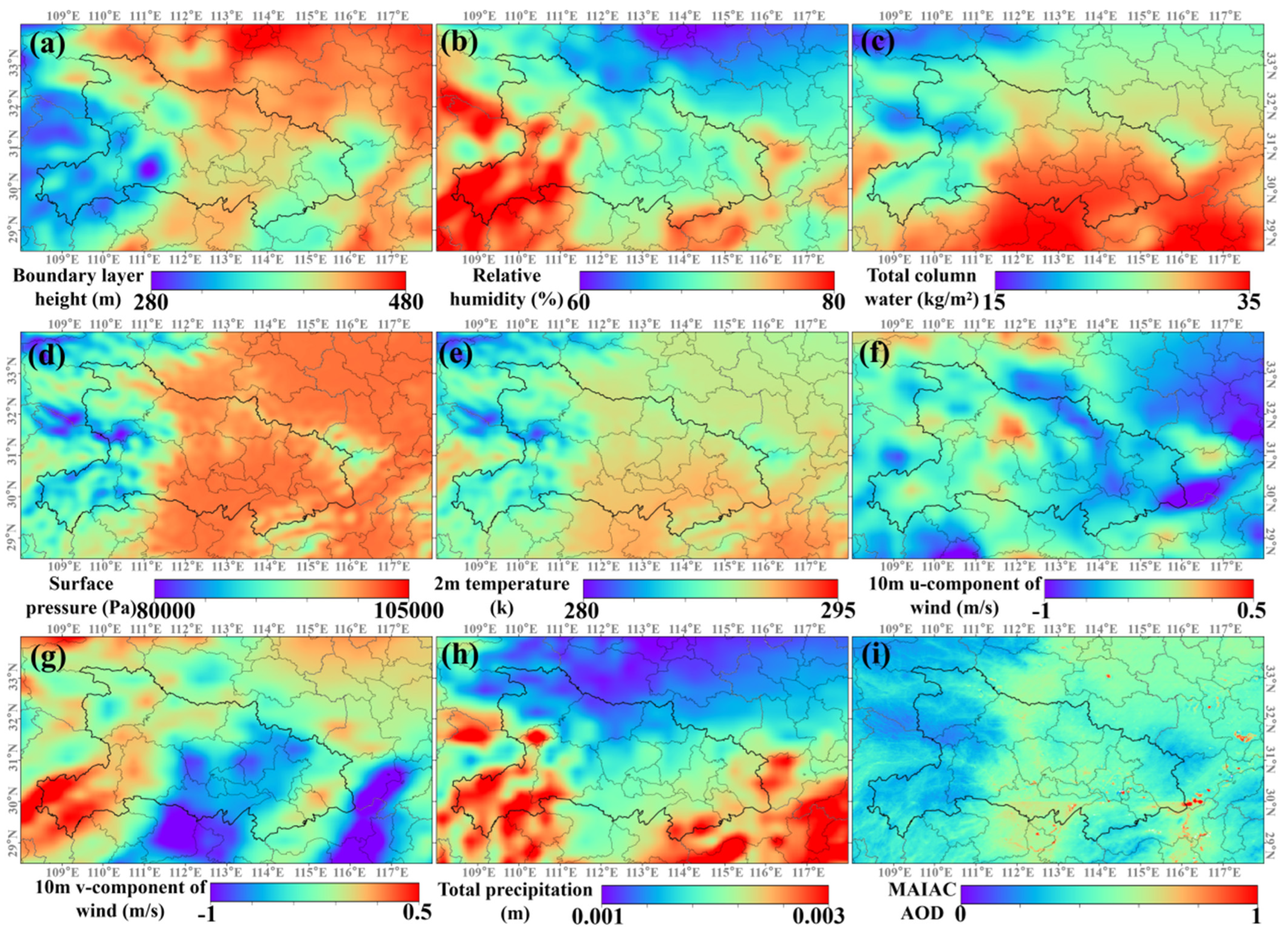
2.2.3. Meteorological Fields

The ERA5, representing the fifth generation of reanalysis datasets, boasts a spatial and temporal resolution of 0.625° × 0.5°/1 h and stands as a comprehensive global dataset disseminated by the European Centre for Medium-Range Weather Forecasts (ECMWF) [26]. A notable extension of this dataset, the ERA5-Land product, elevates the accuracy of ERA5’s land surface parameters by providing a more detailed spatial resolution of 0.1° × 0.1° [27]. This specialized dataset lays a particular emphasis on the land surface characteristics, thus yielding higher quality data.

For the purpose of this study, we sourced a variety of parameters from both ERA5 and ERA5-Land (accessible via CDS, at http://cds.climate.copernicus.eu, accessed on 25 July 2023), each demonstrating significant correlations with aerosols [28,29,30]. These parameters, instrumental in the reconstruction of aerosol optical depth (AOD) and the estimation of PM_2.5, include the boundary layer height (blh), total column water (tcw), relative humidity (rh), surface pressure (sp), total precipitation (tp), the 10 m u-component of wind (u10), the 10 m v-component of wind (v10), and the 2 m temperature (t2m).

2.2.4. Additional Data

The SRTM Version 3 Digital Elevation Model (DEM) dataset, unveiled by the National Aeronautics and Space Administration (NASA) in January 2015, has garnered considerable acclaim for its precision and widespread adoption as one of the most preferred DEMs available [31]. This study utilizes the SRTM DEM Version 3 with a grid resolution of 1 km, obtained from the Resources and Environmental Science and Data Center of the Chinese Academy of Sciences (http://www.resdc.cn, accessed on 25 July 2023). The data, and its representative usage, are illustrated in Figure 1.

Nighttime light remote sensing offers a unique methodology for assessing nocturnal terrestrial environments and human activities, by discerning faint sources of light emissions after sundown. We leverage this nighttime light data to evaluate the extent of human activity, which, in turn, aids in the estimation of PM_2.5 levels. The research utilizes annual nighttime light data (NTL), gathered over the course of 2015 to 2020, which carries a spatial resolution of 15 arc-seconds. This dataset was acquired from the study by Chen et al. [32] (https://doi.org/10.7910/DVN/YGIVCD, accessed on 25 July 2023).

In addition to the above, the study also incorporates annual population data from 2015 to 2020, carrying a spatial resolution of 1 × 1 km. This data, sourced from Worldpop [33] (https://www.worldpop.org/, accessed on 25 July 2023), facilitates the assessment of PM_2.5 exposure risk as weighted by population density, a key focus area of this research.

2.2.5. Data Reprocessing

In the present study, our initial focus was on refining the datasets to include only geographical coordinates ranging from 108°E to 118°E and from 28.5°N to 34°N. This strategic decision effectively restricted our study area to Hubei Province. Following this initial step, we subjected the trimmed datasets to a uniform interpolation process. The result was a refined resolution of 0.01° × 0.01° (550 × 1000), thus ensuring consistency across all the datasets. The subsequent phase of our research involved the organization and combination of the hourly datasets—for instance, meteorological variables and MERRA2 AOD—on a daily basis. This collation process was performed using a simple yet effective daily averaging method. Here, we computed the mean value for each variable over a span of 24 h, adhering to Beijing time (East 8). This approach enabled us to standardize our data and pave the way for further utilization.

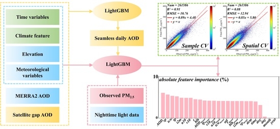
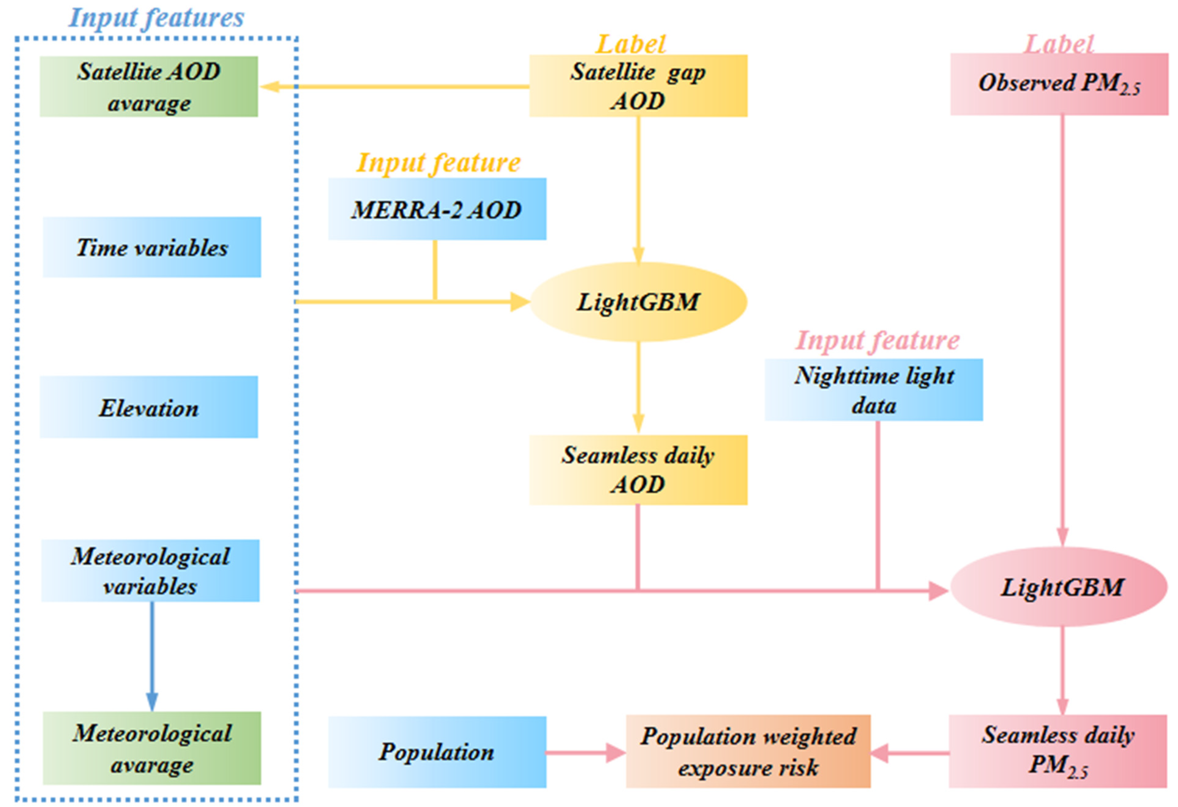
2.3. The Framework of This Study

2.3.1. Climate Feature

Yang et al. [15] indicated that the utilization of geolocation information (specifically latitude and longitude) within a decision-tree model can result in spatial discontinuities in the resulting dataset. This happens because grids with identical latitude or longitude may be assigned identical values during the mapping process, thus leading to the aforementioned spatial discontinuities. Addressing this issue, our study puts forward a novel methodology that uses climatic features as an alternative to latitude and longitude to account for spatial proximity. Particularly, we leverage average meteorological data and MAIAC AOD averages (as depicted in Figure 3) to represent climate features. The distinctiveness of these climatic features fluctuates in relation to their respective spatial distances, thus allowing them to act as effective substitutes for longitude and latitude values.

To clarify, meteorological data in themselves do not inherently contain geolocation information. For instance, the temperature of 30 °C does not have any hidden geolocation information. Hence, previous studies have employed latitude and longitude to convey geolocation information (such as [time, lon, lat, and mete]). Our study diverges from this norm by utilizing the mean values of multiple meteorological variables instead of geographic coordinates (such as [time, climate feature, and mete]). These mean values, indicative of climatic characteristics, enable us to evaluate the spatial proximity of two points based on the closeness of their respective meteorological means, rather than the geographic distance derived from latitude and longitude. Therefore, we are circumventing the limitation Yang et al. [15] mentioned via the utilization of the climate feature.

2.3.2. LightGBM

The Light Gradient Boosting Machine (LightGBM) is a highly esteemed gradient boosting framework, notable for its outstanding performance, efficiency, and accuracy [34]. Developed by Microsoft, it utilizes a unique algorithm designed to expedite training and handle large-scale datasets more proficiently. The distinguishing characteristic of LightGBM is its leaf-wise growth strategy. This approach prioritizes the expansion of leaves that possess the most significant potential for loss reduction when constructing decision trees.

Furthermore, LightGBM introduces advanced features, such as histogram-based binning and exclusive feature bundling, amplifying its predictive prowess. The strategic optimizations adopted by LightGBM offer numerous advantages, encompassing shorter training durations, less memory consumption, and enhanced model performance. Given these attributes, LightGBM is particularly suited for applications that necessitate precise predictions and can process substantial data volumes [35].

In this study, we capitalize on the efficacy of LightGBM for the reconstruction of aerosol optical depth (AOD) and PM_2.5 estimation, demonstrating its capability to manage complex datasets efficiently. To ascertain the optimal set of hyperparameters for LightGBM, an exhaustive range of values was assessed. Specific hyperparameters, including n_estimators (ranging from 2 to 500), max_depth (from 4 to 20), num_leaves (from 5 to 128), subsample (from 0.1 to 0.99), colsample_bytree (from 0.1 to 0.99), and learning_rate (from 0.01 to 0.5), were optimized employing the Bayesian optimization algorithm [36]. This approach was taken to ensure the achievement of the highest possible model performance.

2.3.3. AOD Reconstruction and PM_2.5 Estimation

Currently, the availability of satellite AOD data is restricted due to spatial gaps caused by factors such as cloud cover, rainy weather, and other causes. To overcome this limitation, this study integrates climate features, elevation, meteorological variables, and MERRA-2 AOD as input features of LightGBM. The MAIAC AOD is used as the training label with the objective of filling in the missing values in the MAIAC AOD. The reconstructed AOD dataset plays a critical role in accurate seamless PM_2.5 estimation.

To evaluate the benefits of incorporating climate feature in PM_2.5 estimation, three distinct scenarios (see

Table 1. Summary of designed PM_2.5 estimation cases.

Cases	Input Features	Label
Baseline	Time, DEM, NTL, METE, AOD	PM2.5
+Geolocation	Time, Geolocation, DEM, NTL, METE, AOD
+Climate feature	Time, Climate feature, DEM, NTL, METE, AOD

Note: DEM is the elevation; NTL is the nighttime light data; METE is the 8-variable meteorological matrix; AOD is the reconstructed seamless AOD; Time refers to the year, month, day, DOY (day of the year, 1 to 365/366) and cumulative day (c-day, 1 to 2192); latitude and longitude are Geolocation information; Climate feature is the collection of meteorological mean data and MAIAC average AOD.

) were developed with the help of reconstructed AOD. The overall methodology employed in this research is illustrated in Figure 4, outlining the framework of our study. Our study aims to improve the reliability of PM_2.5 estimation, contributing to a better understanding of air pollution dynamics and its impact on public health.

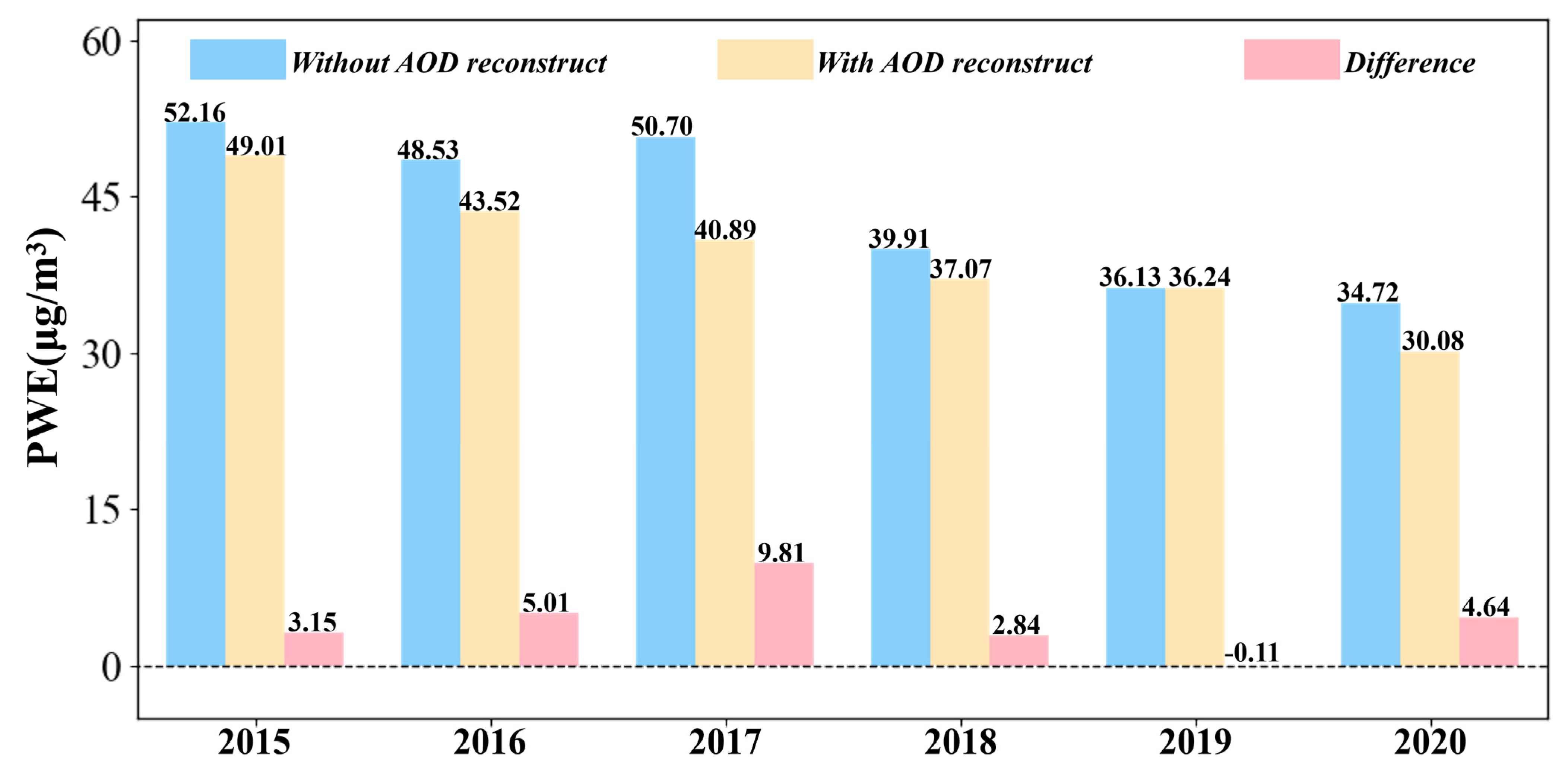
2.3.4. Population-Weighted Exposure

To demonstrate the significance of AOD reconstruction, this study will compare the disparities in assessing population-weighted exposure risk between the gap PM_2.5 datasets constructed by MAIAC AOD and the seamless PM_2.5 datasets constructed by reconstructed AOD. The population-weighted exposure (PWE) can be calculated using the formula below [37].

$$\mathrm{P}\mathrm{W}\mathrm{E}={\displaystyle {\sum }_{\mathrm{i}=1}^{\mathrm{n}}({\mathrm{P}}_{\mathrm{i}}\times {\mathrm{C}}_{\mathrm{i}}})/{\displaystyle {\sum }_{\mathrm{i}=1}^{\mathrm{n}}{\mathrm{P}}_{\mathrm{i}}},$$

(2)

where the P_i is the population in grid i. C_i is the PM_2.5 concentration in grid i.

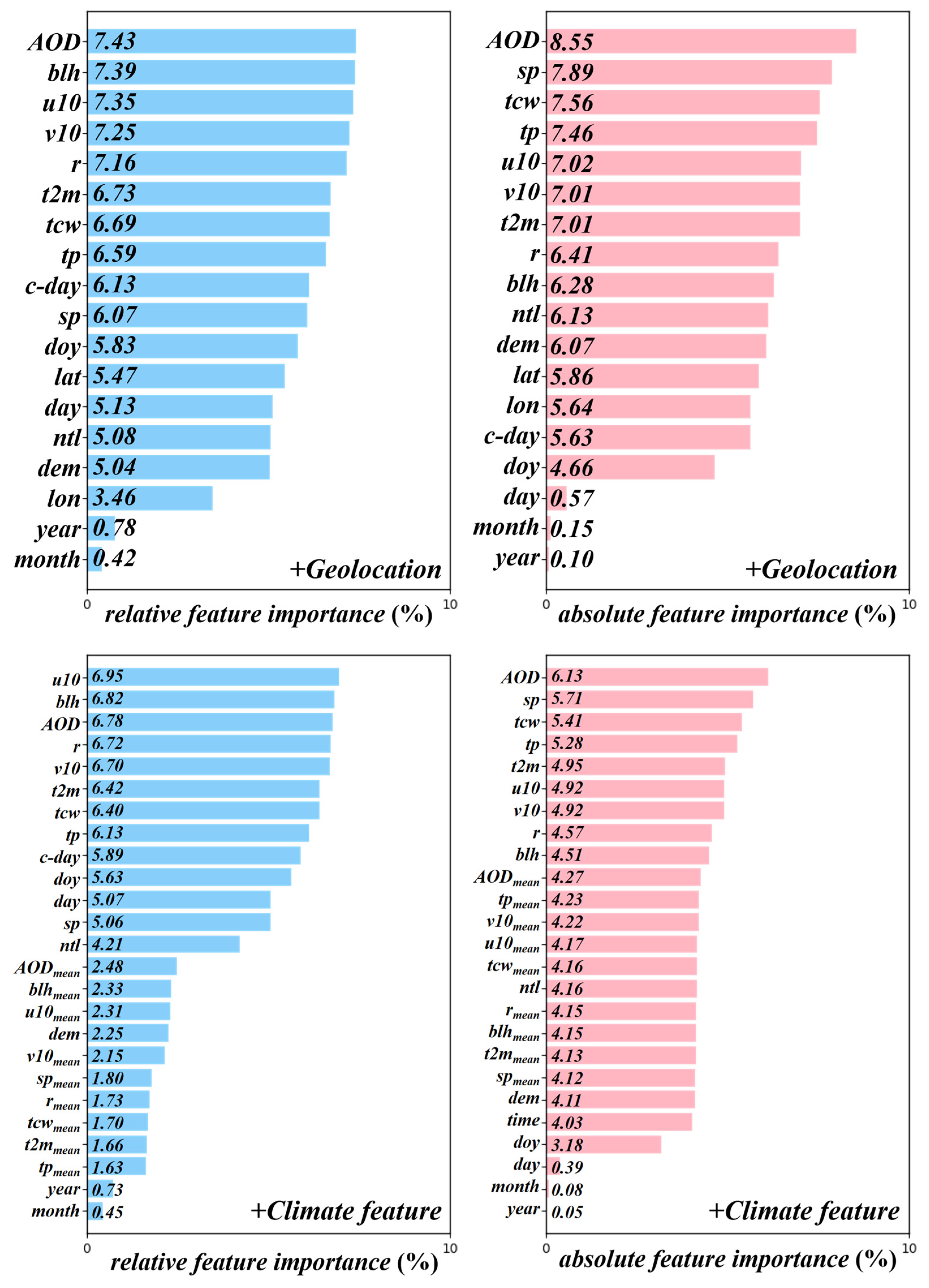
2.3.5. Random Permutation Method for Calculating Absolute Feature Importance

The LightGBM incorporates the relative feature importance attribute that evaluates the significance of input features by using metrics, e.g., the average depth of input features across multiple base models or the number of feature splits in the base models. However, this approach disregards the interactions among input features. This study will use a random permutation method for calculating absolute feature importance to explain the input feature contributions. The specific calculation method is outlined below.

(1)

The whole sample was divided into two parts, with a ratio of 9:1. The training set consisted of 90% of the data, while the remaining 10% was allocated for testing;

(2)

An initial LightGBM model is constructed and its performance on the validation set (mean absolute percentage error, MAPE) is recorded as the baseline performance.

$$\mathrm{M}\mathrm{A}\mathrm{P}{\mathrm{E}}_{\mathrm{b}\mathrm{a}\mathrm{s}\mathrm{e}\mathrm{l}\mathrm{i}\mathrm{n}\mathrm{e}}=\frac{1}{\mathrm{n}}{\displaystyle {\sum }_{\mathrm{i}=1}^{\mathrm{n}}\left|\frac{{\mathrm{x}}_{\mathrm{i}}-{\mathrm{y}}_{\mathrm{i}}}{{\mathrm{x}}_{\mathrm{i}}}\right|}\times 100\%,$$

(3)

where n represents the total number of test records, x_i represents the i_th record of actual value, and y_i represents the i_th record of predicted value;

(3)

For each feature, its value is randomly shuffled and the model’s performance on the testing set is recomputed.

$$\mathrm{M}\mathrm{A}\mathrm{P}{\mathrm{E}}_{\mathrm{s}\mathrm{h}\mathrm{u}\mathrm{f}\mathrm{f}\mathrm{l}\mathrm{e}}=\frac{1}{\mathrm{n}}{\displaystyle {\sum }_{\mathrm{i}=1}^{\mathrm{n}}\left|\frac{{\mathrm{x}}_{\mathrm{i}}-{\mathrm{z}}_{\mathrm{i}}}{{\mathrm{x}}_{\mathrm{i}}}\right|}\times 100\%,$$

(4)

where z_i represents the i_th record of repredicted value;

(4)

The feature importance score can be determined using the following formula.

feature signficance_j = MAPE_shuffle − MAPE_baseline,

(5)

$${\mathrm{absolute}\mathrm{feature}\mathrm{importance}}_{\mathrm{j}}{=\mathrm{feature}\mathrm{signficance}}_{\mathrm{j}}/{\displaystyle {\sum }_{\mathrm{i}=1}^{\mathrm{m}}{\mathrm{feature}\mathrm{signficance}}_{\mathrm{i}}}$$

(6)

where m represents the total number of input features.

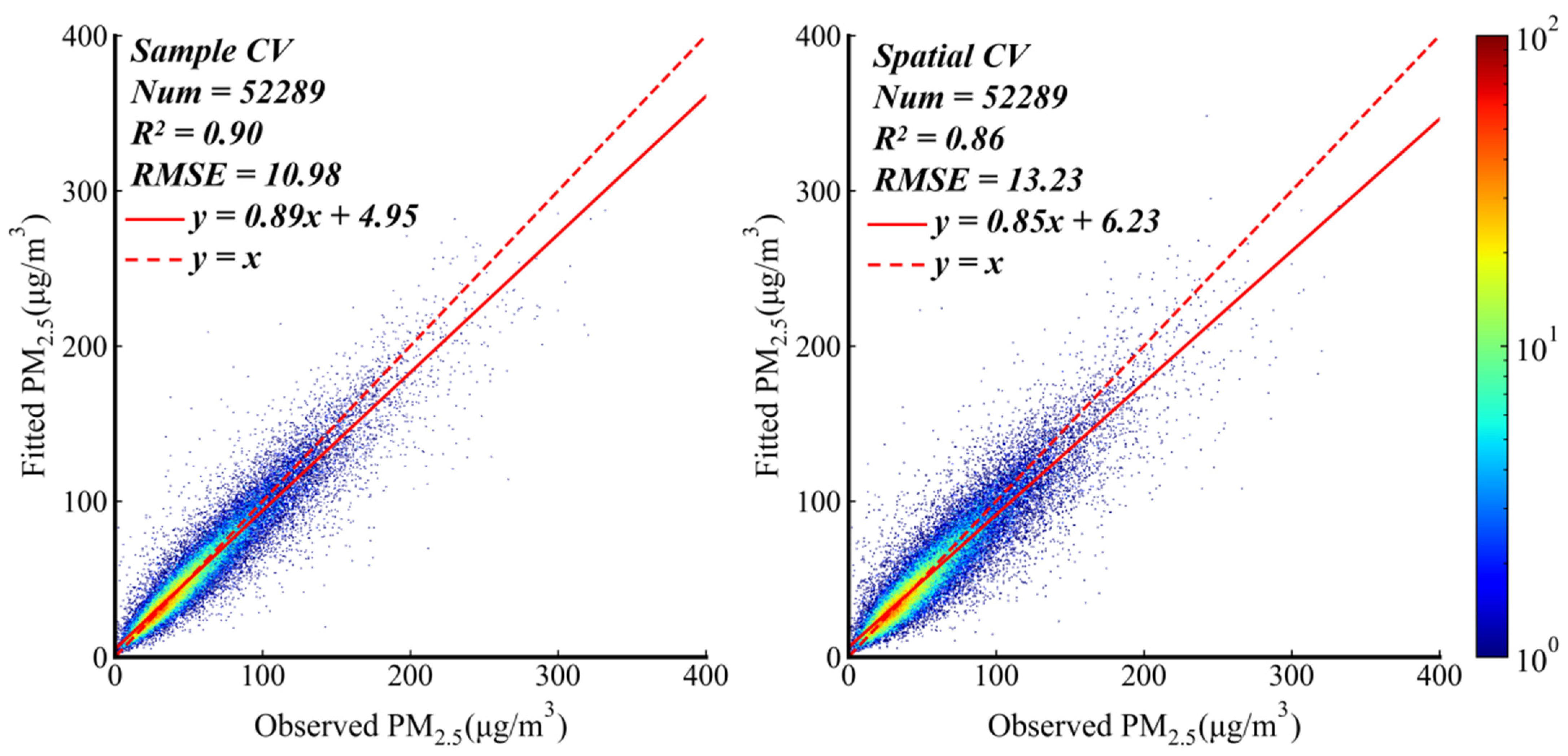
2.4. Model Performance Evaluation

The 10-fold sample/spatial cross-validation (CV) approach was employed to assess the precision of PM_2.5 estimation in this study. Specifically, the sample/spatial CV was repeated ten times, each iteration reserving 10% of the samples/sites for testing purposes while utilizing the remaining 90% for training. The model’s overall performance was evaluated by combining the results from all ten test runs and utilizing the R² (coefficient of determination) and RMSE (root mean square error) metrics.

$${\mathrm{R}}^2=1-{\displaystyle {\sum }_{\mathrm{i}=1}^{\mathrm{n}}({\mathrm{x}}_{\mathrm{i}}-{\mathrm{y}}_{\mathrm{i}}}{)}^2/{\displaystyle {\sum }_{\mathrm{i}=1}^{\mathrm{n}}({\mathrm{x}}_{\mathrm{i}}-\overline{\mathrm{x}}}{)}^2,$$

(7)

$$\mathrm{R}\mathrm{M}\mathrm{S}\mathrm{E}=\sqrt{\frac{1}{\mathrm{n}}{\displaystyle {\sum }_{\mathrm{i}=1}^{\mathrm{n}}({\mathrm{x}}_{\mathrm{i}}-{\mathrm{y}}_{\mathrm{i}}}{)}^2}$$

(8)

where n represents the total number of test records, x_i represents the i_th record of actual value, y_i represents the i_th record of estimated value, and $\stackrel{-}{\mathrm{x}}$ represents the mean of the total actual value.

3. Results

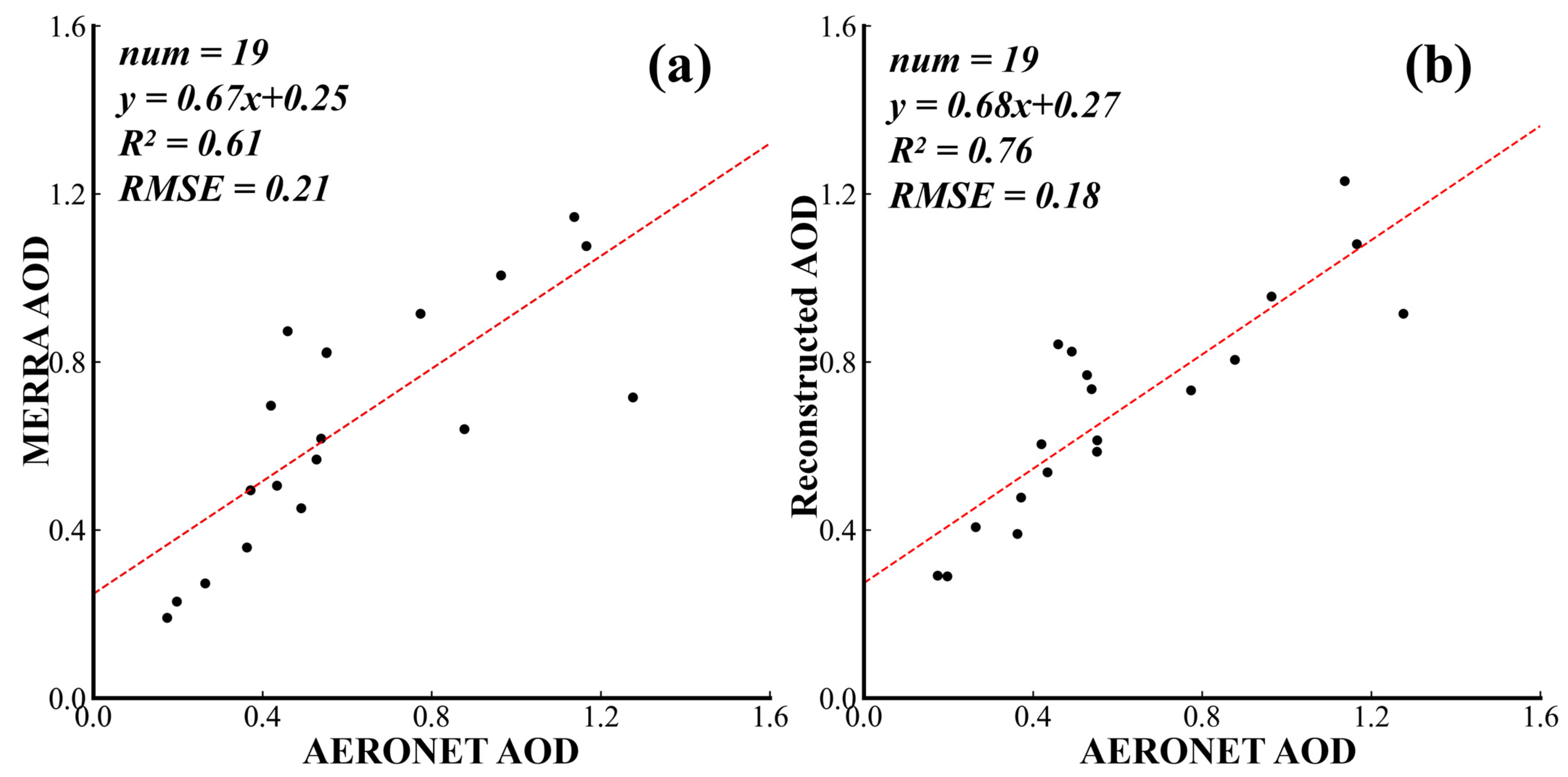
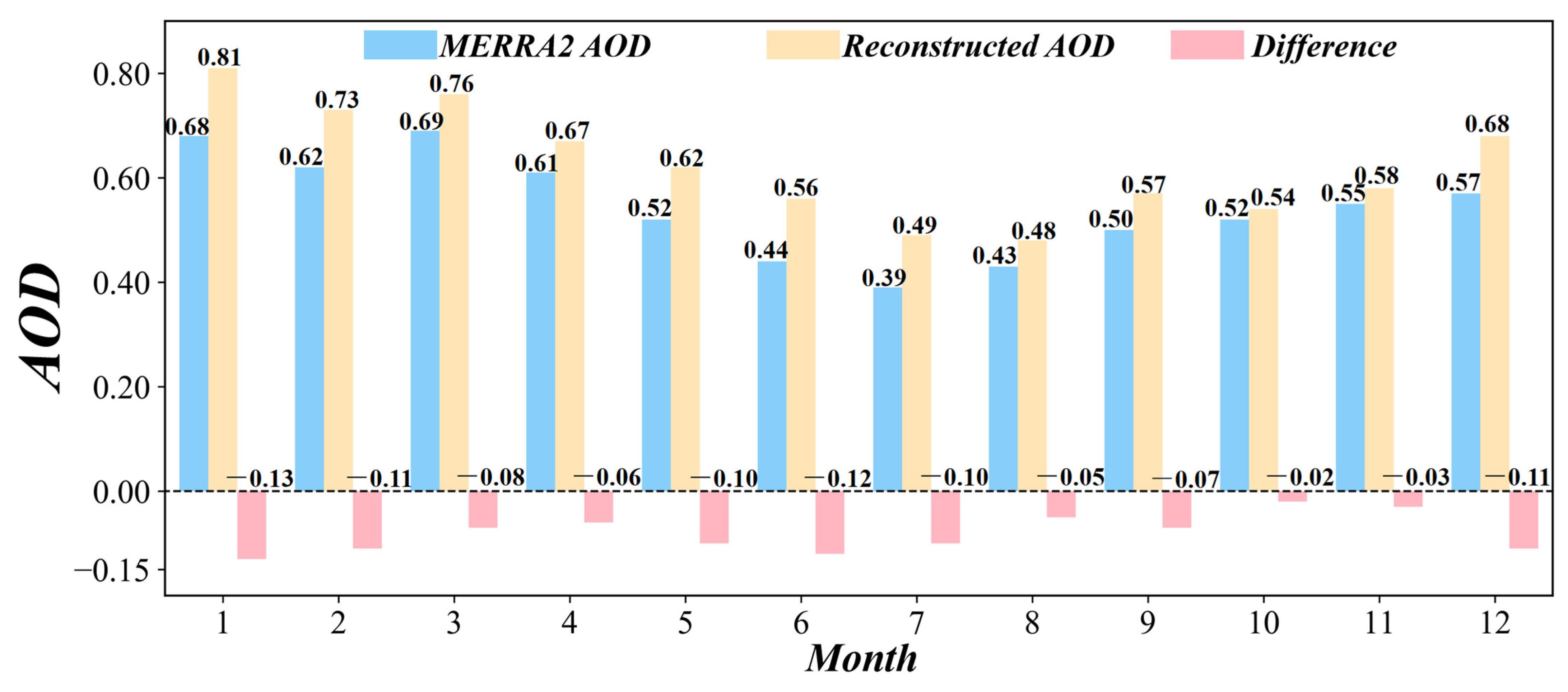
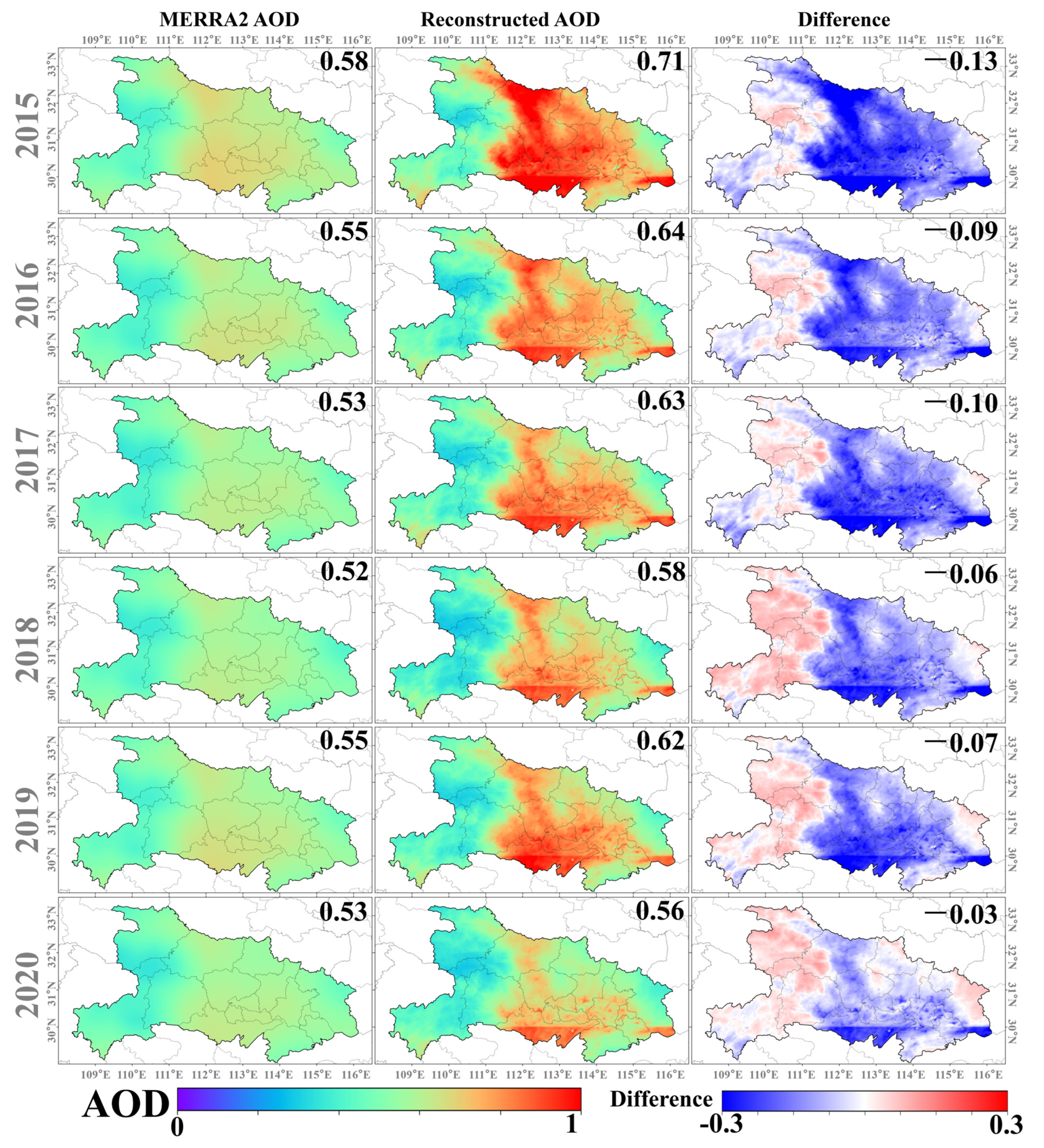
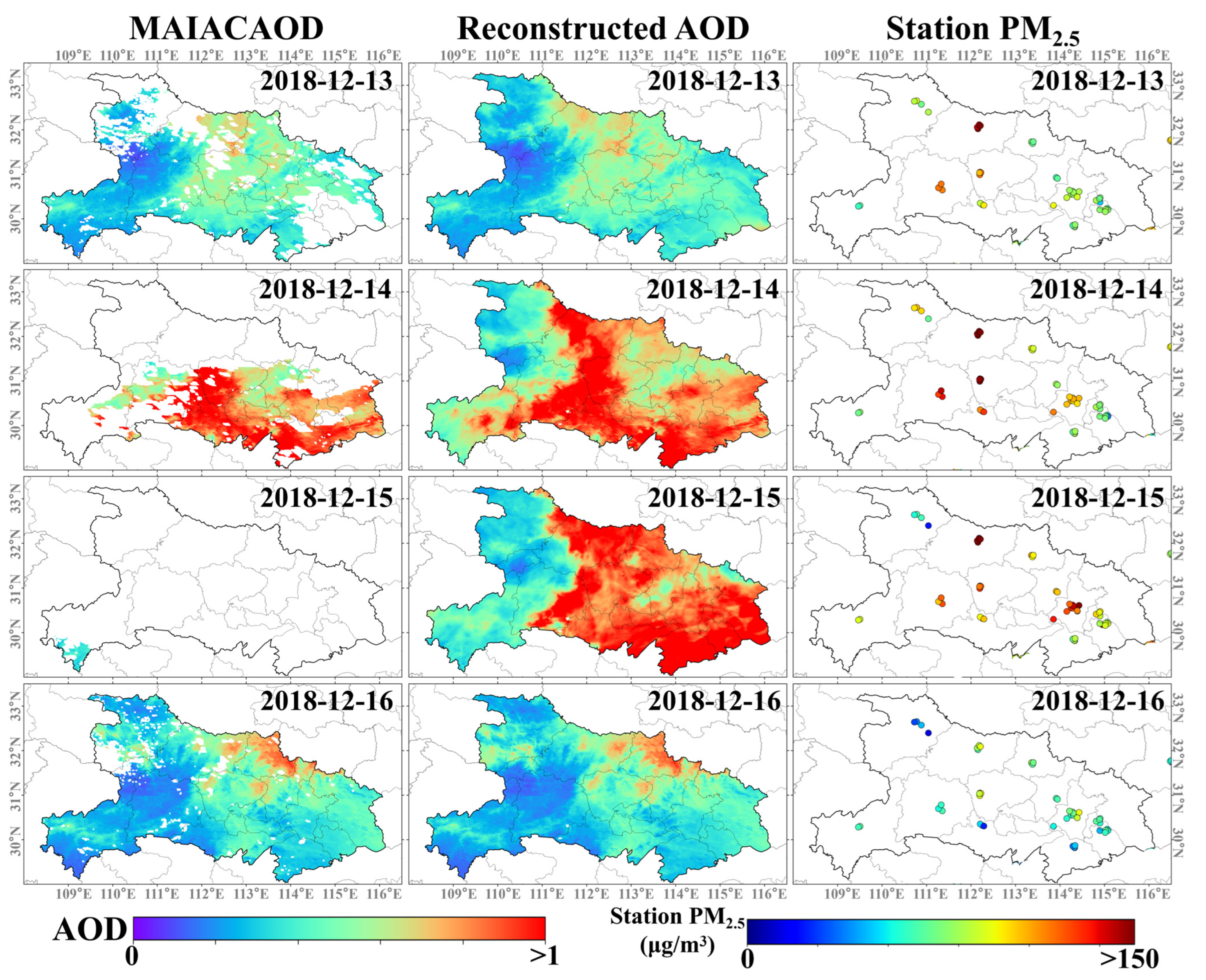
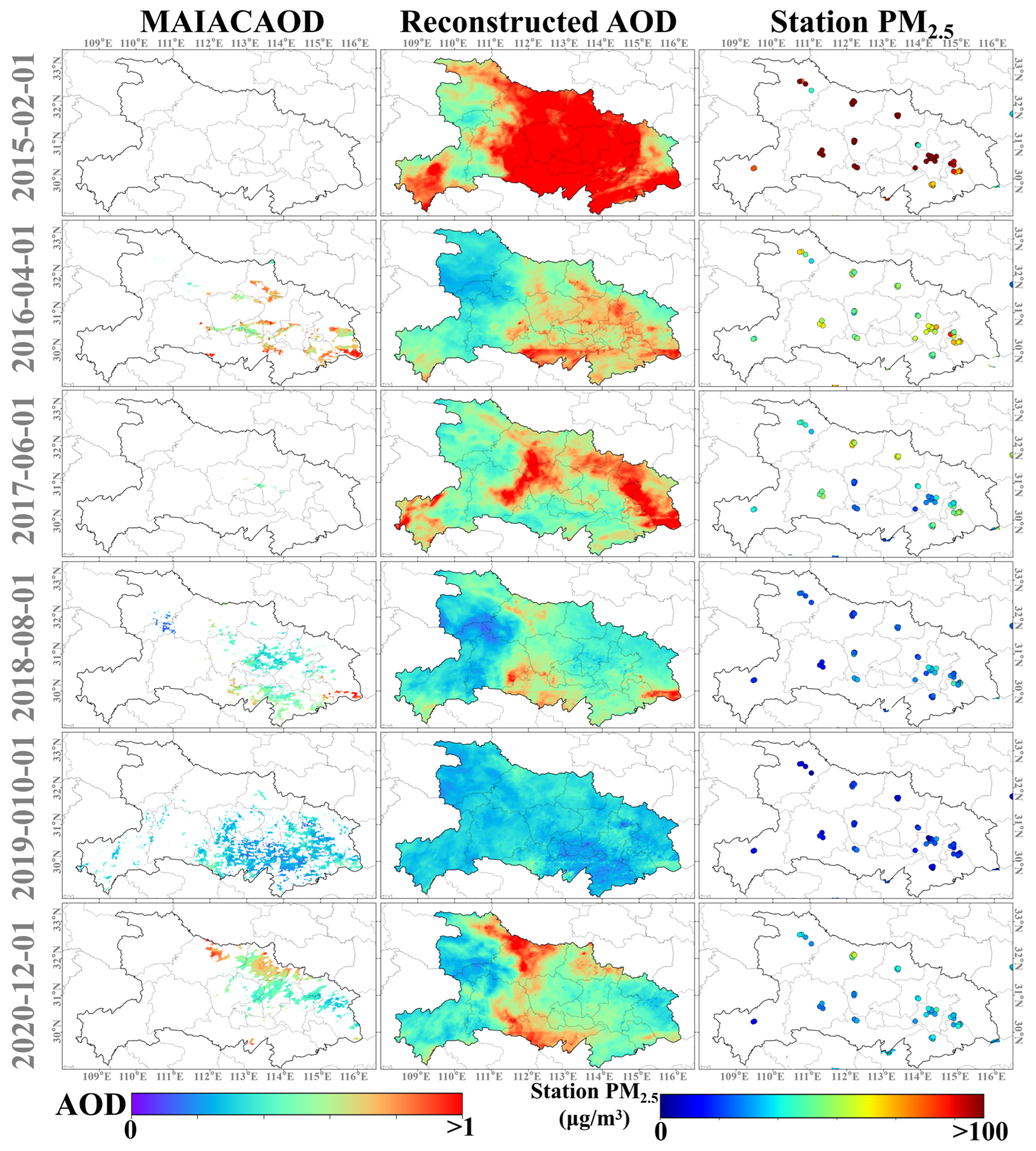
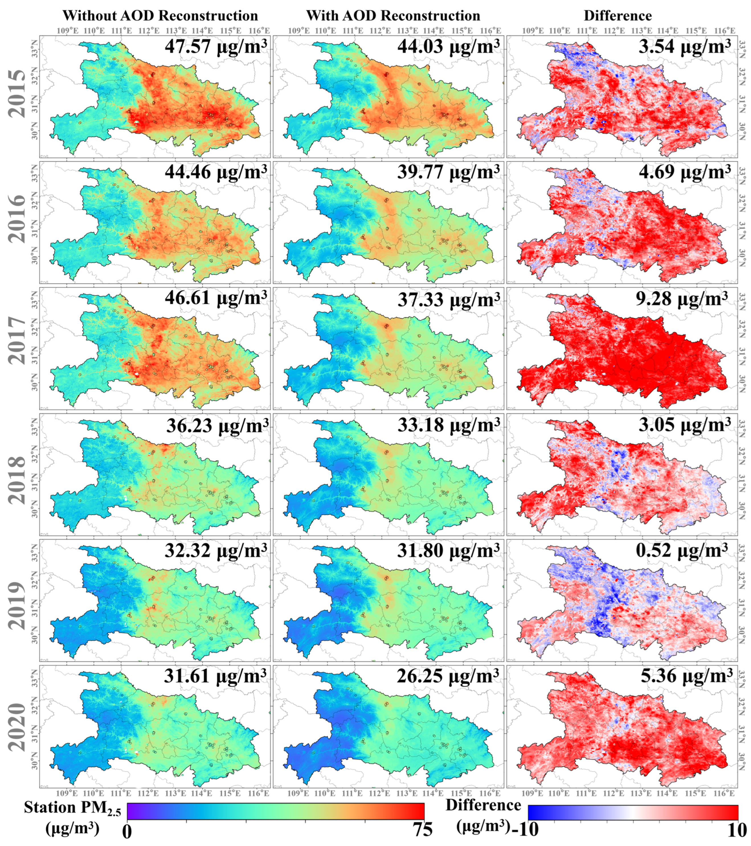
3.1. AOD Reconstruction

Figure 5 illustrates the scatter plot comparing AERONET AOD with MERRA2 AOD (Figure 5a) and reconstructed AOD (Figure 5b). The reconstructed AOD, with an R²/RMSE of 0.76/0.18, surpassing the better performance of MERRA2 AOD (R²/RMSE = 0.61/0.21) by 0.15 in R² and −0.03 in RMSE. Based on the AOD reconstruction, this study produced a seamless daily AOD dataset for Hubei Province, spanning 1 January 2015 to 31 December 2020, at a spatial resolution of 0.01° × 0.01°. Additionally, as shown in Figure 6, the reconstructed AOD exhibited higher monthly mean values compared to MERRA2 AOD, with a difference ranging from 0.02 to 0.13. Regarding the spatial distribution of the annual average AOD (Figure 7), the reconstructed AOD was notably higher than MERRA2 AOD in the Jianghan Plain (~0.15 higher); while in the western mountainous regions, the reconstructed AOD was considerably lower than the MERRA2 AOD (~0.10 lower).

Figure 8 provides an example of gapped and reconstructed daily AOD, demonstrating a significant haze event occurring over a 4-day period. It is worth noting that the original AOD data contained substantial gaps, especially on 15 December 2018, coinciding with the highest PM_2.5 observations. These gaps were a result of the declouding process. Through the AOD reconstruction process, this study successfully restored this high AOD event, capturing intricate small-scale features, which can be attributed to the integration of meteorological information and MERRA2 AOD. Furthermore, as Figure 9 shows, we provide a comparison between MODIS AOD and the reconstructed AOD on the 1st of February 2015, April 2016, June 2017, August 2018, October 2019, and December 2020. This comparison also effectively demonstrates the performance of our reconstruction across various days, seasons, and years.

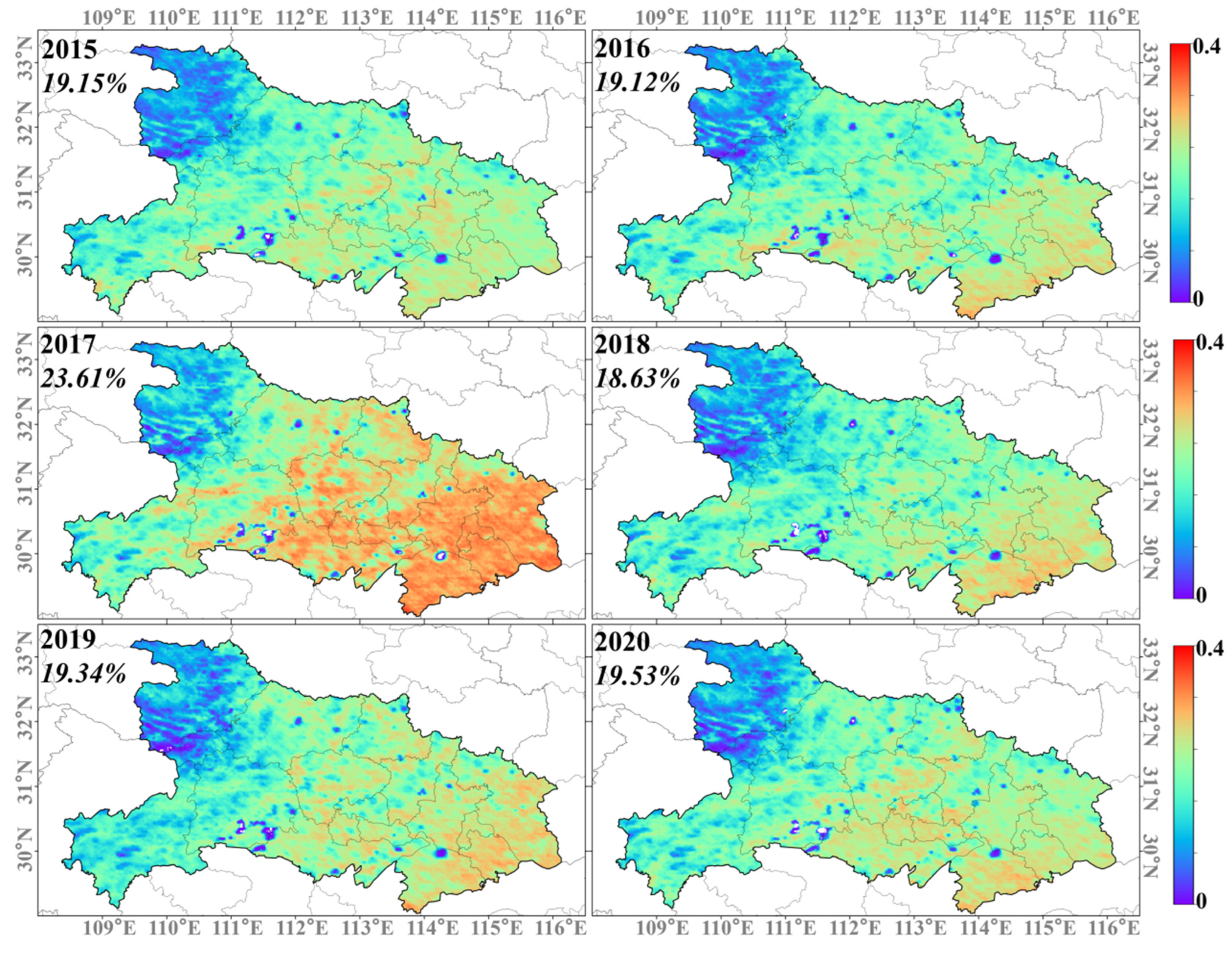
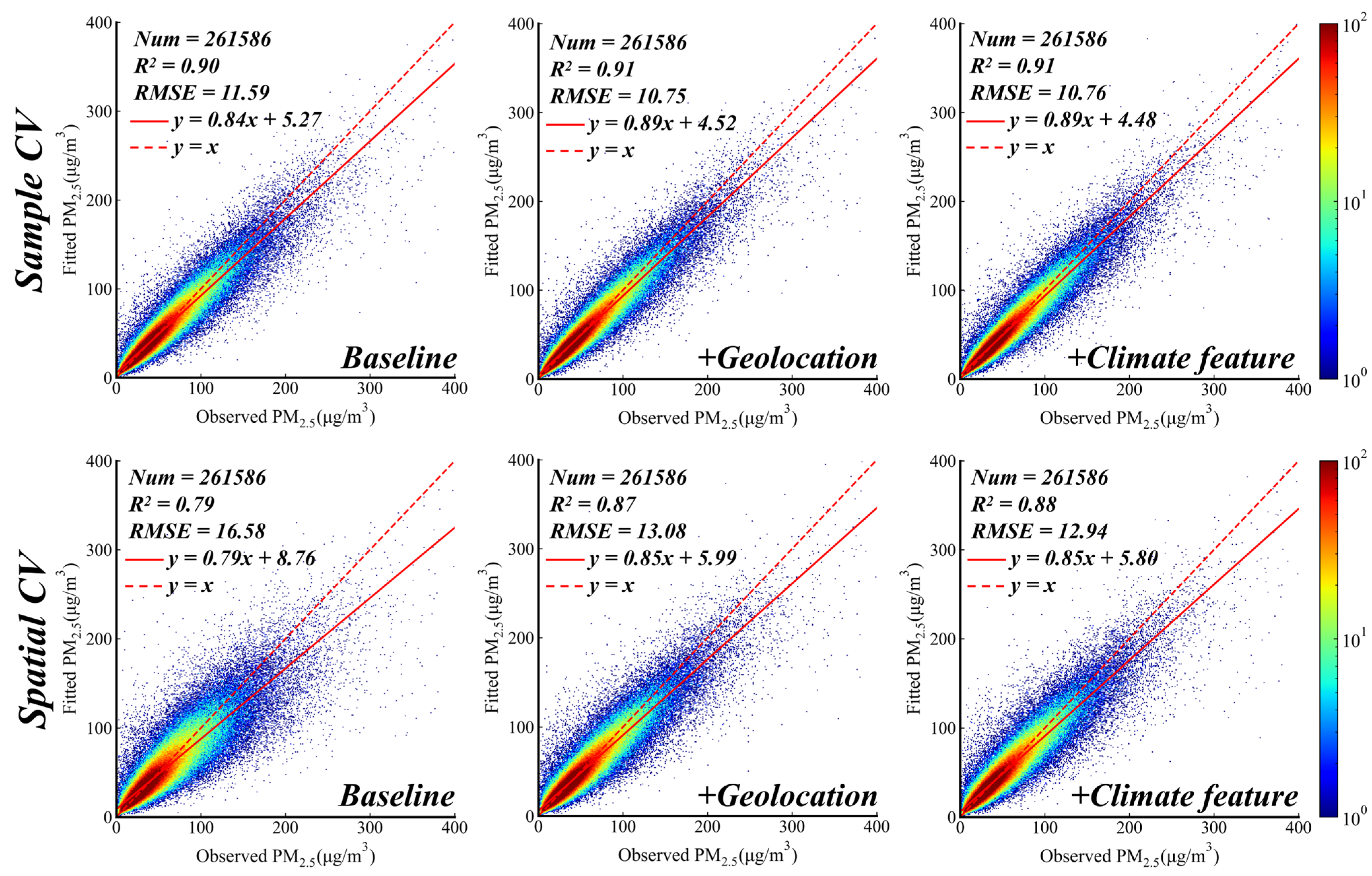
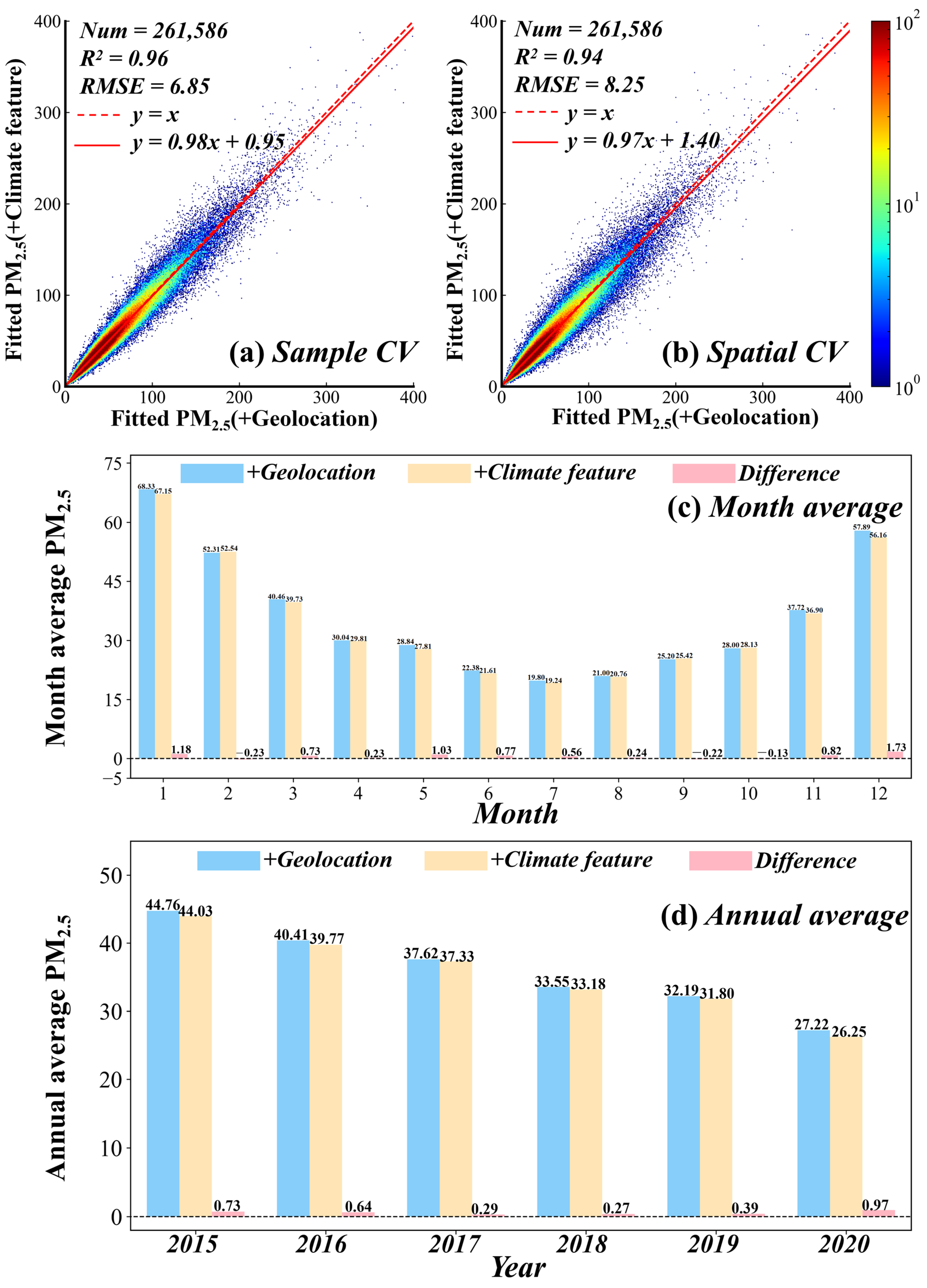
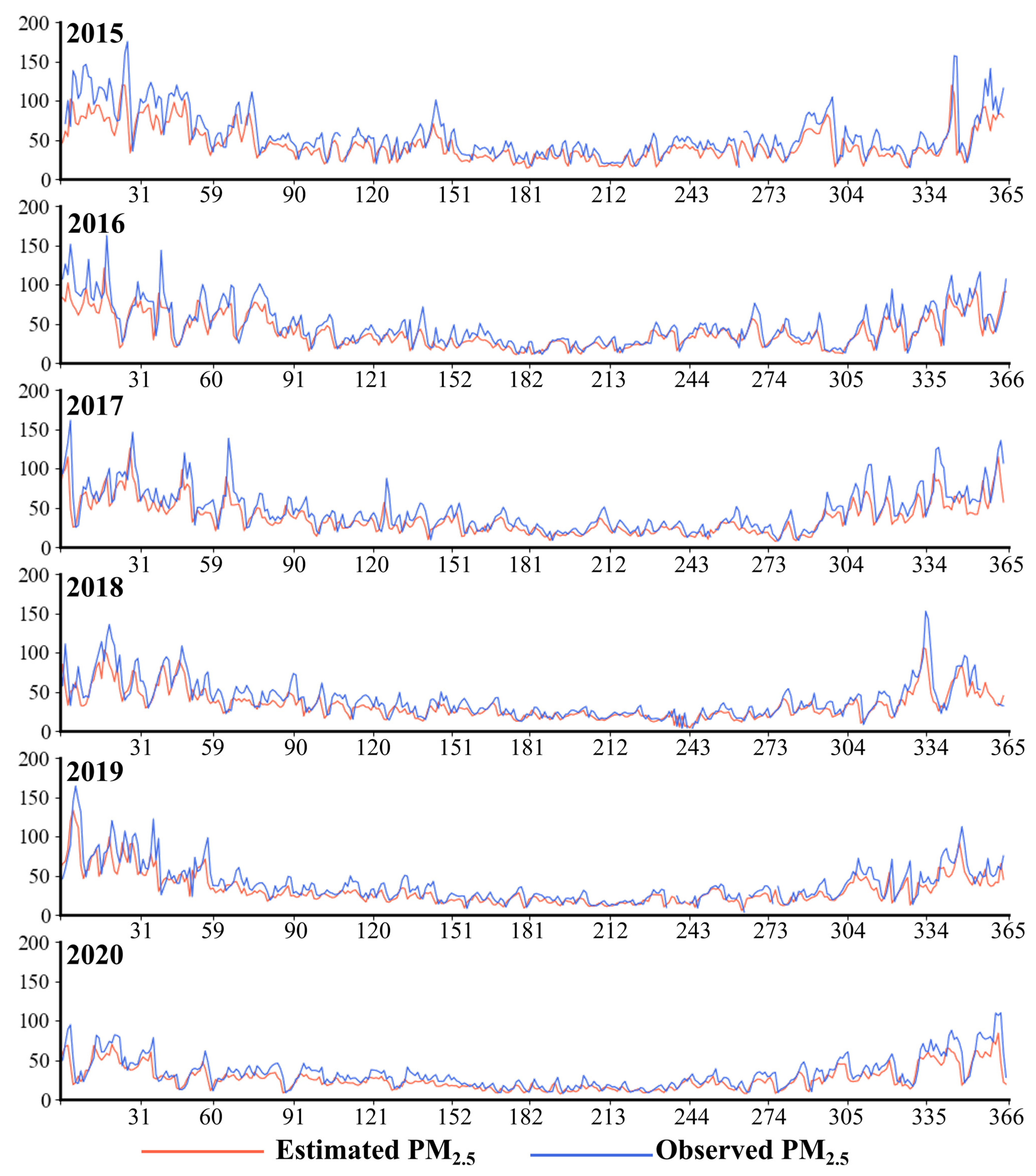
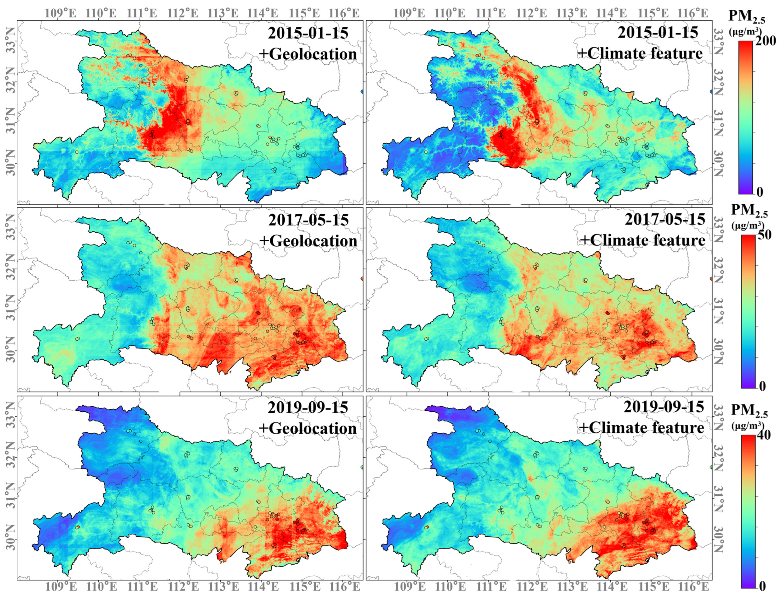
3.2. PM_2.5 Estimation

The 10-fold sample/spatial CV results of different PM_2.5 estimation experiments (introduced in Table 1) are presented in Figure 10. The baseline represents the control case without the geolocation (longitude and latitude) information or climate feature. In comparing the baseline with the sample CV, which reflects the model interpolation capability, it is observed that the geolocation or climate feature played a negligible role in PM_2.5 estimation (R²: increased from 0.90 to 0.91/0.91, RMSE: reduced from 11.59 to 10.75/10.76 µg/m³). Compared with Huang et al.’s [38] study (sample CV-R2/RMSR = 0.89/13.10 µg/m³), our model performed better. However, under spatial CV, which reflects the model extrapolation capability, the geolocation or climate features demonstrated significant importance in PM_2.5 estimation (R²: increased from 0.79 to 0.87/0.88, RMSE: reduced from 16.58 to 13.08/12.94 µg/m³). This phenomenon indicates the crucial role of geolocation information or climate feature in estimating PM_2.5 over out-station areas. The difference between the geolocation-based model and the climate-feature-based model was found to be insignificant. Figure 11a,b illustrates that both models yield similar results in terms of the sample (R² = 0.96) and spatial CV (R² = 0.94). Furthermore, the disparities observed in the monthly (−0.23~1.73 µg/m³, Figure 11c) or annual (0.29~0.97 µg/m³, Figure 11d) averages of the datasets produced by the geolocation-based model and the climate-feature-based model are minimal. Figure 12 shows the comparison between the daily PM_2.5 from the air-quality station and the estimated daily PM_2.5 by our proposed method. The daily PM_2.5 from the air-quality station is significantly higher than the estimated PM_2.5, due to the fact that most of the air-quality monitoring stations are located in urban areas with severe air pollution.

However, if the latitude and longitude contribute highly to the estimation model, grids with identical longitude or latitude values may receive the same value during the mapping process and lead to spatial discontinuities in produced PM_2.5 dataset. Figure 13 presents examples of estimated PM_2.5 using geolocation information (left column) on 15 January 2015, 15 May 2017, and 15 September 2019, which display multiple spatial discontinuities. Conversely, the images generated using climate features (right column) do not exhibit this problem. Hence, employing the climate feature instead of geolocation information as the input feature ensures the produced PM_2.5 dataset with higher quality.

4. Discussion

Previous studies [18,19] have commonly utilized the relative feature-importance attribute from machine-learning models to assess the significance of input features. This attribute is obtained through an ensemble approach that evaluates hyperparameters such as n_estimators and max_depth in base models. However, the relative feature importance calculated ignores the interactions between input features. To address this limitation, we proposed a method for calculating absolute feature importance, which combines the random permutation method [39] with MAPE (mean absolute percentage error).

As shown in Figure 14, the most important input feature in absolute/relative feature importance is AOD/u10. This difference is due to the fact that the relative feature importance is influenced by the interaction between the input features, i.e., the input features are increasing and decreasing in the same way or in the opposite way. Hence, the absolute feature importance is more accurate for describing the significance of the input features to the estimated model.

Under the relative feature importance, the top three important features in both the geolocation-based model and the climate-feature-based model are AOD (7.43%/6.78%), blh (7.39%/6.82%), and u10 (7.35%/6.95%). The order of these features differs between the two models but the differences are minimal (0.08%/0.17%), making it challenging to determine which input feature is explicitly the most important, while under the absolute feature importance, there is greater variability (0.99%/0.72%). Additionally, in both the geolocation-based and climate-feature-based models, AOD (8.55%/6.13%), sp (7.89%/5.71%), and tcw (7.56%/5.41%) occupied the top three of absolute feature importance, which indicates that the absolute feature importance is more able to explain the feature contributions.

On the other hand, to demonstrate the significance of AOD reconstruction, we compared the annual mean difference between two datasets: the gap PM_2.5 dataset (generated without AOD reconstruction, model performance depicted in Figure 15, sample/spatial CV R² = 0.90/0.86) and the seamless PM_2.5 dataset (produced with AOD reconstruction). From 2015 to 2020, the gap PM_2.5 dataset (left column in Figure 16) displayed higher average values (0.52~9.28 µg/m³) compared to the seamless PM_2.5 dataset (center column in Figure 16). The most substantial difference (9.28 µg/m³) was observed in 2017, which can be attributed to the higher AOD coverage (as shown in Figure 2, the AOD availability rate in 2017 exceeded 4%, surpassing other years). The annual average PM_2.5 values fluctuated downwards under the gap PM_2.5 dataset for the period of 2015 to 2020. However, under the seamless PM_2.5 dataset, the annual average PM_2.5 levels in Hubei Province exhibited a consistent decrease each year. Moreover, the variation in annual mean PM_2.5 values (0.52~9.28 µg/m³, right column in Figure 16) also significantly contributed to disparities in the population-exposure risk (−0.11~9.81 µg/m³, as shown in Figure 17). Hence, AOD reconstruction is crucial for the accurate estimation of PM_2.5 levels and the assessment of exposure risk.

5. Conclusions

In this research, we successfully employed the AOD reconstruction method, combined with MERRA AOD, meteorological elements, elevation, and other variables, to interpolate the missing values of MAIAC AOD. Following this, we utilized the reconstructed AOD dataset, which demonstrated an R² of 0.76 compared to AERONET AOD, to derive seamless daily average PM_2.5 concentrations across Hubei Province from 2015 to 2020. Our study emphasizes the utility of incorporating climate features as inputs for PM_2.5 concentration estimation, steering away from the traditional dependence on latitude and longitude data. This strategy mitigates the potential for spatial discontinuity that may arise from latitude and longitude discrepancies, ensuring a more precise PM_2.5 estimation, with a sample/space cross-validation R² of 0.91/0.88.

Moreover, our study introduces a novel method for evaluating the absolute feature importance of machine-learning models. In contrast to the relative feature-importance characteristics inherent in most machine-learning models, where the top three features display a nonsignificant difference of 0.08%/0.17%, our proposed method offers a more nuanced and stable interpretation of feature significance to the model, as evidenced by the substantial difference of 0.99%/0.72% for the top three features. Furthermore, our research discovered that AOD reconstruction can mitigate the overestimation of annual average PM_2.5 concentrations (ranging from 0.52 to 9.28 µg/m³) and decrease the bias in exposure risk assessment (ranging from −0.11 to 9.81 µg/m³).

In conclusion, our results underscore the efficacy of the AOD reconstruction technique in interpolating missing AOD values and estimating PM_2.5 concentrations. Through the incorporation of climate features and the implementation of the absolute feature-importance method, we have enhanced the spatial continuity, accuracy, and interpretability of the PM_2.5 estimations. These improvements amplify our understanding of air pollution dynamics and can aid in devising targeted interventions for improving air quality. Further research should investigate the applicability of this approach in different geographical contexts and evaluate its potential for wider deployment in air-quality monitoring and management systems.

References

1. Xu, L.; Chen, B.; Huang, C.; Zhou, M.; You, S.; Jiang, F.; Chen, W.; Deng, J. Identifying PM2.5-Related Health Burden in the Context of the Integrated Development of Urban Agglomeration Using Remote Sensing and GEMM Model. Remote Sens. 2023, 15, 2770. [Google Scholar] [CrossRef]
2. Kangas, T.; Gadeyne, S.; Lefebvre, W.; Vanpoucke, C.; Rodriguez-Loureiro, L. Are air quality perception and PM2.5 exposure differently associated with cardiovascular and respiratory disease mortality in Brussels? Findings from a census-based study. Environ. Res. 2023, 219, 115180. [Google Scholar] [CrossRef]
3. Krittanawong, C.; Qadeer, Y.K.; Hayes, R.B.; Wang, Z.; Virani, S.; Thurston, G.D.; Lavie, C.J. PM2.5 and Cardiovascular Health Risks. Curr. Probl. Cardiol. 2023, 48, 101670. [Google Scholar] [CrossRef] [PubMed]
4. Zhu, Y.; Shi, Y. Spatio-temporal variations of PM2.5 concentrations and related premature deaths in Asia, Africa, and Europe from 2000 to 2018. Environ. Impact Assess. Rev. 2023, 99, 107046. [Google Scholar] [CrossRef]
5. Bai, H.; Gao, W.; Seong, M.; Yan, R.; Wei, J.; Liu, C. Evaluating and optimizing PM2.5 stations in Yangtze River Delta from a spatial representativeness perspective. Appl. Geogr. 2023, 154, 102949. [Google Scholar] [CrossRef]
6. Wang, Y.; Xu, G.; Chen, L.; Chen, K. Characteristics of Air Pollutant Distribution and Sources in the East China Sea and the Yellow Sea in Spring Based on Multiple Observation Methods. Remote Sens. 2023, 15, 3262. [Google Scholar] [CrossRef]
7. Buya, S.; Usanavasin, S.; Gokon, H.; Karnjana, J. An Estimation of Daily PM2.5 Concentration in Thailand Using Satellite Data at 1-Kilometer Resolution. Sustainability 2023, 15, 10024. [Google Scholar] [CrossRef]
8. Lin, J.; Zhang, A.; Chen, W.; Lin, M. Estimates of Daily PM2.5 Exposure in Beijing Using Spatio-Temporal Kriging Model. Sustainability 2018, 10, 2772. [Google Scholar] [CrossRef] [Green Version]
9. Choi, K.; Chong, K. Modified Inverse Distance Weighting Interpolation for Particulate Matter Estimation and Mapping. Atmosphere 2022, 13, 846. [Google Scholar] [CrossRef]
10. Kim, D.; Jeon, W.; Park, J.; Mun, J.; Choi, H.; Kim, C.-H.; Lee, H.-J.; Jo, H.-Y. A Numerical Analysis of the Changes in O3 Concentration in a Wildfire Plume. Remote Sens. 2022, 14, 4549. [Google Scholar] [CrossRef]
11. Qi, L.; Zheng, H.; Ding, D.; Wang, S. Effects of Anthropogenic Emission Control and Meteorology Changes on the Inter-Annual Variations of PM2.5–AOD Relationship in China. Remote Sens. 2022, 14, 4683. [Google Scholar] [CrossRef]
12. Bai, K.; Li, K.; Sun, Y.; Wu, L.; Zhang, Y.; Chang, N.-B.; Li, Z. Global synthesis of two decades of research on improving PM2.5 estimation models from remote sensing and data science perspectives. Earth-Sci. Rev. 2023, 241, 104461. [Google Scholar] [CrossRef]
13. Chen, A.; Yang, J.; He, Y.; Yuan, Q.; Li, Z.; Zhu, L. High spatiotemporal resolution estimation of AOD from Himawari-8 using an ensemble machine learning gap-filling method. Sci. Total Environ. 2023, 857, 159673. [Google Scholar] [CrossRef] [PubMed]
14. Li, L.; Franklin, M.; Girguis, M.; Lurmann, F.; Wu, J.; Pavlovic, N.; Breton, C.; Gilliland, F.; Habre, R. Spatiotemporal imputation of MAIAC AOD using deep learning with downscaling. Remote Sens. Environ. 2020, 237, 111584. [Google Scholar] [CrossRef]
15. Yang, Q.; Yuan, Q.; Li, T. Ultrahigh-resolution PM2.5 estimation from top-of-atmosphere reflectance with machine learning: Theories, methods, and applications. Environ. Pollut. 2022, 306, 119347. [Google Scholar] [CrossRef]
16. Liu, Z.; Xiao, Q.; Li, R. Full Coverage Hourly PM2.5 Concentrations’ Estimation Using Himawari-8 and MERRA-2 AODs in China. Int. J. Environ. Res. Public Health 2023, 20, 1490. [Google Scholar] [CrossRef]
17. Geng, G.; Zhang, Q.; Martin, R.V.; van Donkelaar, A.; Huo, H.; Che, H.; Lin, J.; He, K. Estimating long-term PM2.5 concentrations in China using satellite-based aerosol optical depth and a chemical transport model. Remote Sens. Environ. 2015, 166, 262–270. [Google Scholar] [CrossRef]
18. Peng, J.; Han, H.; Yi, Y.; Huang, H.; Xie, L. Machine learning and deep learning modeling and simulation for predicting PM2.5 concentrations. Chemosphere 2022, 308, 136353. [Google Scholar] [CrossRef]
19. Hao, X.; Hu, X.; Liu, T.; Wang, C.; Wang, L. Estimating urban PM2.5 concentration: An analysis on the nonlinear effects of explanatory variables based on gradient boosted regression tree. Urban Clim. 2022, 44, 101172. [Google Scholar] [CrossRef]
20. Fisher, A.; Rudin, C.; Dominici, F. All Models are Wrong, but Many are Useful: Learning a Variable’s Importance by Studying an Entire Class of Prediction Models Simultaneously. J. Mach. Learn. Res. 2019, 20, 1–81. [Google Scholar] [CrossRef]
21. Li, R.; Mei, X.; Wei, L.; Han, X.; Zhang, M.; Jing, Y. Study on the contribution of transport to PM2.5 in typical regions of China using the regional air quality model RAMS-CMAQ. Atmos. Environ. 2019, 214, 116856. [Google Scholar] [CrossRef]
22. Xu, M.; Weng, Z.; Xie, Y.; Chen, B. Environment and health co-benefits of vehicle emission control policy in Hubei, China. Transp. Res. Part D Transp. Environ. 2023, 120, 103773. [Google Scholar] [CrossRef]
23. Lyapustin, A.; Wang, Y.; Korkin, S.; Huang, D. MODIS Collection 6 MAIAC algorithm. Atmos. Meas. Tech. 2018, 11, 5741–5765. [Google Scholar] [CrossRef] [Green Version]
24. Randles, C.A.; da Silva, A.M.; Buchard, V.; Colarco, P.R.; Darmenov, A.; Govindaraju, R.; Smirnov, A.; Holben, B.; Ferrare, R.; Hair, J.; et al. The MERRA-2 Aerosol Reanalysis, 1980 Onward. Part I: System Description and Data Assimilation Evaluation. J. Clim. 2017, 30, 6823–6850. [Google Scholar] [CrossRef]
25. Ding, Y.; Chen, Z.; Lu, W.; Wang, X. A CatBoost approach with wavelet decomposition to improve satellite-derived high-resolution PM2.5 estimates in Beijing-Tianjin-Hebei. Atmos. Environ. 2021, 249, 118212. [Google Scholar] [CrossRef]
26. Hersbach, H.; Bell, B.; Berrisford, P.; Hirahara, S.; Horányi, A.; Muñoz-Sabater, J.; Nicolas, J.; Peubey, C.; Radu, R.; Schepers, D.; et al. The ERA5 global reanalysis. Q. J. R. Meteorol. Soc. 2020, 146, 1999–2049. [Google Scholar] [CrossRef]
27. Muñoz-Sabater, J.; Dutra, E.; Agustí-Panareda, A.; Albergel, C.; Arduini, G.; Balsamo, G.; Boussetta, S.; Choulga, M.; Harrigan, S.; Hersbach, H.; et al. ERA5-Land: A state-of-the-art global reanalysis dataset for land applications. Earth Syst. Sci. Data 2021, 13, 4349–4383. [Google Scholar] [CrossRef]
28. Chen, S.; Tong, B.; Russell, L.M.; Wei, J.; Guo, J.; Mao, F.; Liu, D.; Huang, Z.; Xie, Y.; Qi, B.; et al. Lidar-based daytime boundary layer height variation and impact on the regional satellite-based PM2.5 estimate. Remote Sens. Environ. 2022, 281, 113224. [Google Scholar] [CrossRef]
29. de Leeuw, G.; Kang, H.; Fan, C.; Li, Z.; Fang, C.; Zhang, Y. Meteorological and anthropogenic contributions to changes in the Aerosol Optical Depth (AOD) over China during the last decade. Atmos. Environ. 2023, 301, 119676. [Google Scholar] [CrossRef]
30. Li, Y.; Chen, Q.; Zhao, H.; Wang, L.; Tao, R. Variations in PM10, PM2.5 and PM1.0 in an Urban Area of the Sichuan Basin and Their Relation to Meteorological Factors. Atmosphere 2015, 6, 150–163. [Google Scholar] [CrossRef] [Green Version]
31. González-Moradas, M.d.R.; Viveen, W. Evaluation of ASTER GDEM2, SRTMv3.0, ALOS AW3D30 and TanDEM-X DEMs for the Peruvian Andes against highly accurate GNSS ground control points and geomorphological-hydrological metrics. Remote Sens. Environ. 2020, 237, 111509. [Google Scholar] [CrossRef]
32. Chen, Z.; Yu, B.; Yang, C.; Zhou, Y.; Yao, S.; Qian, X.; Wang, C.; Wu, B.; Wu, J. An extended time series (2000–2018) of global NPP-VIIRS-like nighttime light data from a cross-sensor calibration. Earth Syst. Sci. Data 2021, 13, 889–906. [Google Scholar] [CrossRef]
33. Tatem, A.J. WorldPop, open data for spatial demography. Sci. Data 2017, 4, 170004. [Google Scholar] [CrossRef] [PubMed]
34. Wang, D.; Zhang, Y.; Zhao, Y. LightGBM: An Effective miRNA Classification Method in Breast Cancer Patients. In Proceedings of the 2017 International Conference on Computational Biology and Bioinformatics, Newark, NJ, USA, 18–20 October 2017; pp. 7–11. [Google Scholar]
35. Hancock, J.; Khoshgoftaar, T.M. Leveraging LightGBM for Categorical Big Data. In Proceedings of the 2021 IEEE Seventh International Conference on Big Data Computing Service and Applications (BigDataService), Oxford, UK, 23–26 August 2021; pp. 149–154. [Google Scholar]
36. Wu, J.; Chen, X.-Y.; Zhang, H.; Xiong, L.-D.; Lei, H.; Deng, S.-H. Hyperparameter Optimization for Machine Learning Models Based on Bayesian Optimizationb. J. Electron. Sci. Technol. 2019, 17, 26–40. [Google Scholar] [CrossRef]
37. Aunan, K.; Ma, Q.; Lund, M.T.; Wang, S. Population-weighted exposure to PM2.5 pollution in China: An integrated approach. Environ. Int. 2018, 120, 111–120. [Google Scholar] [CrossRef]
38. Huang, Y.; Ji, Y.; Zhu, Z.; Zhang, T.; Gong, W.; Xia, X.; Sun, H.; Zhong, X.; Zhou, X.; Chen, D. Satellite-based spatiotemporal trends of ambient PM2.5 concentrations and influential factors in Hubei, Central China. Atmos. Res. 2020, 241, 104929. [Google Scholar] [CrossRef]
39. Breiman, L. Random Forests. Mach. Learn. 2001, 45, 5–32. [Google Scholar] [CrossRef] [Green Version]
Figure 1. Study area map showing 136 PM2.5 recording sites (colorful dots) and elevation (color shading, unit: meters).
Remotesensing 15 03822 g001
Figure 2. Spatial distribution of effective observation rate of MAIAC daily average AOD from 2015 to 2020.
Remotesensing 15 03822 g002
Figure 3. Spatial distribution of climate feature. Climate feature is the collection of the mean of meteorological data and AOD data.
Remotesensing 15 03822 g003
Figure 4. Graphical representation of our study design.
Remotesensing 15 03822 g004
Figure 5. Comparing daily AERONET AOD (as the ground truth) with MERRA2 AOD (a) and reconstructed AOD (b) in Hubei Province.
Remotesensing 15 03822 g005
Figure 6. Comparison of monthly mean of MERRA2 AOD and reconstructed AOD.
Remotesensing 15 03822 g006
Figure 7. Comparison of annual mean of MERRA2 AOD and reconstructed AOD. The spatial discontinuity in the reconstructed AOD around 30°N is attributed to the splicing of MODIS data.
Remotesensing 15 03822 g007
Figure 8. Example of original (left column) and reconstructed (center column) daily AOD from 13 December 2018 to 16 December 2018. The (right column) is the station PM2.5 observations.
Remotesensing 15 03822 g008
Figure 9. Example of original (left column) and reconstructed (center column) daily AOD on 1 February 2015, 1 April 2016, 1 June 2017, 1 August 2018, 1 October 2019, and 1 December 2020. The (right column) is the station PM2.5 observations.
Remotesensing 15 03822 g009
Figure 10. Density scatter plots of 10-fold sample/spatial cross-validation by using different PM2.5 estimation experiments.
Remotesensing 15 03822 g010
Figure 11. Comparison of the model using geographic information and model using climate feature.
Remotesensing 15 03822 g011
Figure 12. Comparison of observed daily PM2.5 from air-quality stations (the daily average of all sites) and estimated PM2.5 by our method (with climate feature, the daily average of the estimated grid dataset).
Remotesensing 15 03822 g012
Figure 13. Comparison of mapping PM2.5 using the geolocation information (left column) and using the climate feature (right column).
Remotesensing 15 03822 g013
Figure 14. Comparison of relative and absolute feature importance.
Remotesensing 15 03822 g014
Figure 15. Density scatter plots of 10-fold sample/spatial cross-validation by using the model with MAIAC AOD rather than reconstructed AOD.
Remotesensing 15 03822 g015
Figure 16. Comparison of annual PM2.5 mean using the gap PM2.5 dataset (produced by MAIAC AOD) and the seamless PM2.5 dataset (produced by reconstructed AOD).
Remotesensing 15 03822 g016
Figure 17. Comparison of population-weighted exposure using the gap PM2.5 dataset (produced by MAIAC AOD) and the seamless PM2.5 dataset (produced by reconstructed AOD).
Remotesensing 15 03822 g017