Article

UniRender: Reconstructing 3D Surfaces from Aerial Images with a Unified Rendering Scheme

1
College of Information and Communication Engineering, Harbin Engineering University, Harbin 150001, China
2
Key Laboratory of Advanced Marine Communication and Information Technology, Ministry of Industry and Information Technology, Harbin Engineering University, Harbin 150001, China
*
Author to whom correspondence should be addressed.
Remote Sens. 2023, 15(18), 4634; https://doi.org/10.3390/rs15184634
Submission received: 26 July 2023 / Revised: 16 September 2023 / Accepted: 18 September 2023 / Published: 21 September 2023

Abstract

:
While recent advances in the field of neural rendering have shown impressive 3D reconstruction performance, it is still a challenge to accurately capture the appearance and geometry of a scene by using neural rendering, especially for remote sensing scenes. This is because both rendering methods, i.e., surface rendering and volume rendering, have their own limitations. Furthermore, when neural rendering is applied to remote sensing scenes, the view sparsity and content complexity that characterize these scenes will severely hinder its performance. In this work, we aim to address these challenges and to make neural rendering techniques available for 3D reconstruction in remote sensing environments. To achieve this, we propose a novel 3D surface reconstruction method called UniRender. UniRender offers three improvements in locating an accurate 3D surface by using neural rendering: (1) unifying surface and volume rendering by employing their strengths while discarding their weaknesses, which enables accurate 3D surface position localization in a coarse-to-fine manner; (2) incorporating photometric consistency constraints during rendering, and utilizing the points reconstructed by structure from motion (SFM) or multi-view stereo (MVS), to constrain reconstructed surfaces, which significantly improves the accuracy of 3D reconstruction; (3) improving the sampling strategy by locating sampling points in the foreground regions where the surface needs to be reconstructed, thus obtaining better detail in the reconstruction results. Extensive experiments demonstrate that UniRender can reconstruct high-quality 3D surfaces in various remote sensing scenes.

Graphical Abstract

1. Introduction

Reconstructing 3D surfaces of a scene from multi-view imagery is one of the key objectives of remote sensing and photogrammetry, as accurate 3D models have a wide range of applications in fields such as urban planning, 3D GPS navigation, and environmental simulation.
Given multi-view input images, traditional surface reconstruction frameworks [1,2,3,4] first use structure-from-motion (SFM) [5] to estimate camera parameters and to reconstruct sparse 3D points.Then, multi-view stereo (MVS) [4,6] is applied, to estimate dense depth maps for each view, and then all the depth maps are fused into a dense point cloud. Finally, the surface reconstruction method, e.g., Poisson surface reconstruction [7], is performed, to reconstruct surface meshes from this point cloud. However, reconstructing complete mesh surfaces from point clouds is challenging, due to the lack of geometric connectivity information. This can lead to incomplete surfaces, particularly in weakly textured or sparse view contexts [8,9]. Additionally, the multi-stage reconstruction pipeline, as opposed to an end-to-end approach, may introduce cumulative errors and noise.
The latest image-based photogrammetry technique, known as neural rendering [8,10,11,12,13,14,15,16,17], employs continuous functions to represent the geometry and appearance of a 3D scene, and it encodes these continuous functions, using neural networks. Additionally, it employs differentiable rendering, to transform the 3D scene into an image, allowing for end-to-end optimization of neural network parameters, by minimizing the disparity between the rendered image and the input image. More specifically, there are two types of rendering manners in neural rendering: surface rendering [8,15,16,17], and volume rendering [13,14,18,19,20,21]. Recent works have tended to use volume rendering to reconstruct 3D surfaces, because it has stronger robustness and is less prone to getting stuck in local minima, compared to surface rendering. However, compared to the impressive performance on indoor datasets, such as DTU [22], high-quality 3D surface reconstruction using volume rendering still remains challenging for remote sensing scenes. A major reason for this dilemma is that the biases that exist in current volume rendering paradigms [13,14,21] are greatly amplified when applied to remote sensing scenes. Furthermore, the view sparsity that characterizes these scenes introduces serious geometric ambiguity.
To address these challenges, and to make neural rendering techniques available for 3D reconstruction in remote sensing, we propose our solution: UniRender, a 3D surface reconstruction method that can achieve high-quality surface reconstruction performance from aerial images. Given a 3D scene described by images, UniRender employs a signed distance field (SDF) [23] to represent the geometry of the scene, and learns the SDF by minimizing the difference between the rendered images and the input images. To achieve precise surface positioning during rendering, we first analyzed the biases that exist in current 3D surface reconstruction methods based on volume rendering [9,13,19,24] and identify the causes of them. Based on this analysis, we designed an approximately unbiased rendering scheme, by naturally unifying surface rendering and volume rendering within a single rendering framework. With such a rendering scheme, UniRender effectively eliminates biases and enables accurate surface position localization in a coarse-to-fine manner. To address the issue of inherent geometric ambiguity in neural rendering, UniRender integrates a geometric constraint mechanism that takes advantage of stereo matching. This mechanism effectively enhances the quality of the reconstructed geometry. Furthermore, to better reconstruct the details of the scene, UniRender adapts a novel spherical sampling algorithm, which can locate the sampling points to the regions that need more attention. In summary, our contribution are as follows:
  • A qualitative and quantitative analysis of the biases that exist in the current volume rendering paradigm.
  • An approximately unbiased rendering scheme.
  • A novel geometric constraint mechanism.
  • A novel spherical sampling algorithm.

2. Related Work

In this section, we offer essential background information on the two primary factors involved in learning 3D geometry from multi-view images using neural rendering: the 3D scene representation and the rendering technique connecting it to 2D observations.

2.1. Neural Implicit Representation

As mentioned in Section 1, traditional multi-view 3D reconstruction frameworks [1,2,3,4] primarily rely on explicit representations, such as point clouds or depth maps, for modeling 3D scenes. These representations are plagued by issues like discretization and limited resolution. By contrast, neural implicit representation [23,25,26] has emerged as an effective solution for 3D geometry and appearance modeling. It leverages continuous implicit functions encoded by neural networks, to represent 3D scenes. Due to its continuity and ability to achieve high spatial resolution, this representation has been widely used. As for learning-based methods, the most commonly used forms are the occupancy field [25] and the signed distance field (SDF) [23].

2.2. 3D Reconstruction with Differentiable Rendering

Unlike traditional photogrammetric techniques [3,4,6,27,28], which treat 3D reconstruction as a cross-view feature matching problem, some approaches [8,13,14,17,19,20,21] treat 3D reconstruction as an inverse rendering problem. They try to estimate the underlying 3D geometry by iteratively rendering the 3D geometry and comparing the rendered image to the input images. The key to this is differentiable rendering [17], which allows the flow of error gradients formed by color differences between the rendered and input images to be back-propagated, thus optimizing the underlying 3D geometry. Depending on the rendering method, we divide these works into two categories: surface rendering and volume rendering.

2.2.1. Surface Rendering

Surface rendering methods [8,15,16,17,29], such as IDR [8], utilize an SDF function encoded by a multi-layer perceptron (MLP), to represent the geometry of a scene. This derives the predicted color from the point where the ray intersects with the surface, which serves as the final rendered color. Subsequently, the MLP is optimized, by using a render loss computed from the rendered color and the color from the input images. However, when propagating backward, the gradient exists only at the surface intersection, leading to a confined spatial receptive field. As a result, these methods usually require mask inputs, to provide additional geometric constraints. Otherwise, the optimization will easily fall into local minima and will produce poor geometric reconstruction.

2.2.2. Density-Field-Based Volume Rendering

By contrast, volume rendering methods [13,14,18,19,20,21] derive the predicted color by integrating colors along the entire ray. Compared to surface rendering, which only optimizes color at a single point, volume rendering benefits from a longer-distance spatial receptive field. NeRF [21] is a typical volume rendering method, but is distinguished by its approach, of treating a 3D scene as a combination of a density field and a color radiance field. It approximates these two fields, using a five-dimensional function encoded by a multi-layer perceptron (MLP). This function takes 3D coordinates and view direction as input and outputs corresponding to volume density and color. By minimizing the discrepancy between the color of the input views and the color estimated through volume rendering using the density field, the density field can learn the correct geometry to satisfy the color constraints from the input views.

2.2.3. SDF-Based Volume Rendering

Despite NeRF [21]’s success in the task of novel view synthesis, the surfaces extracted from the density field are usually noisy [18], and it is difficult to determine a suitable density threshold, to extract the surface from the density field. Therefore, subsequent improvements have attempted to represent scene geometry with an SDF function [23] and have introduced an SDF-induced volume density σ = ψ ( s d f ) , to enable SDF-based volume rendering [13,14]. This approach allows for the extraction of smooth surfaces from the zero set of the SDF.

2.3. Issues Existing in Volume Rendering

Numerous experiments [13,14,24,30] have shown that SDF-based volume rendering is highly beneficial for recovering surfaces from 2D images, especially for indoor datasets like DTU [22]. However, achieving high-quality 3D surface reconstruction still remains challenging for remote sensing scenes, because the biases inherent in current volume rendering paradigms [13,14,21] are greatly amplified when applied to remote sensing scenes. Furthermore, the view sparsity that characterizes these scenes introduces serious geometric ambiguity. More specifically, the biases and ambiguities are as follows:
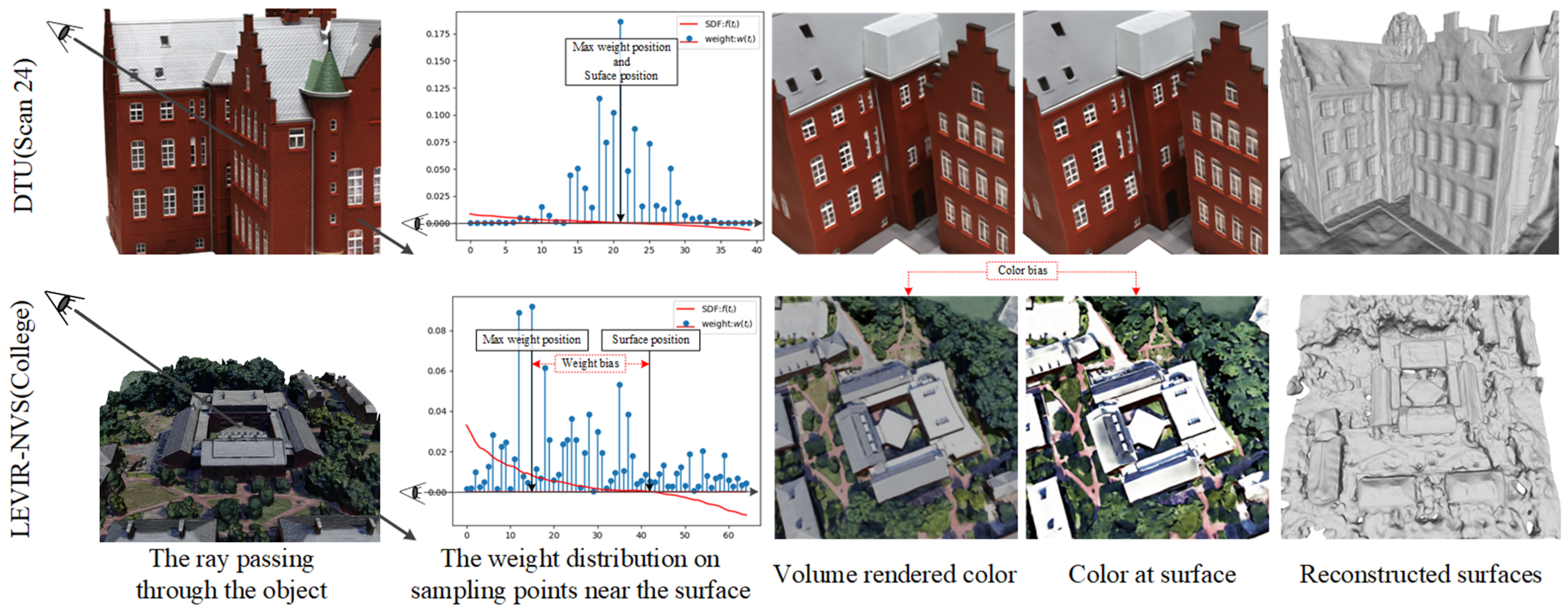
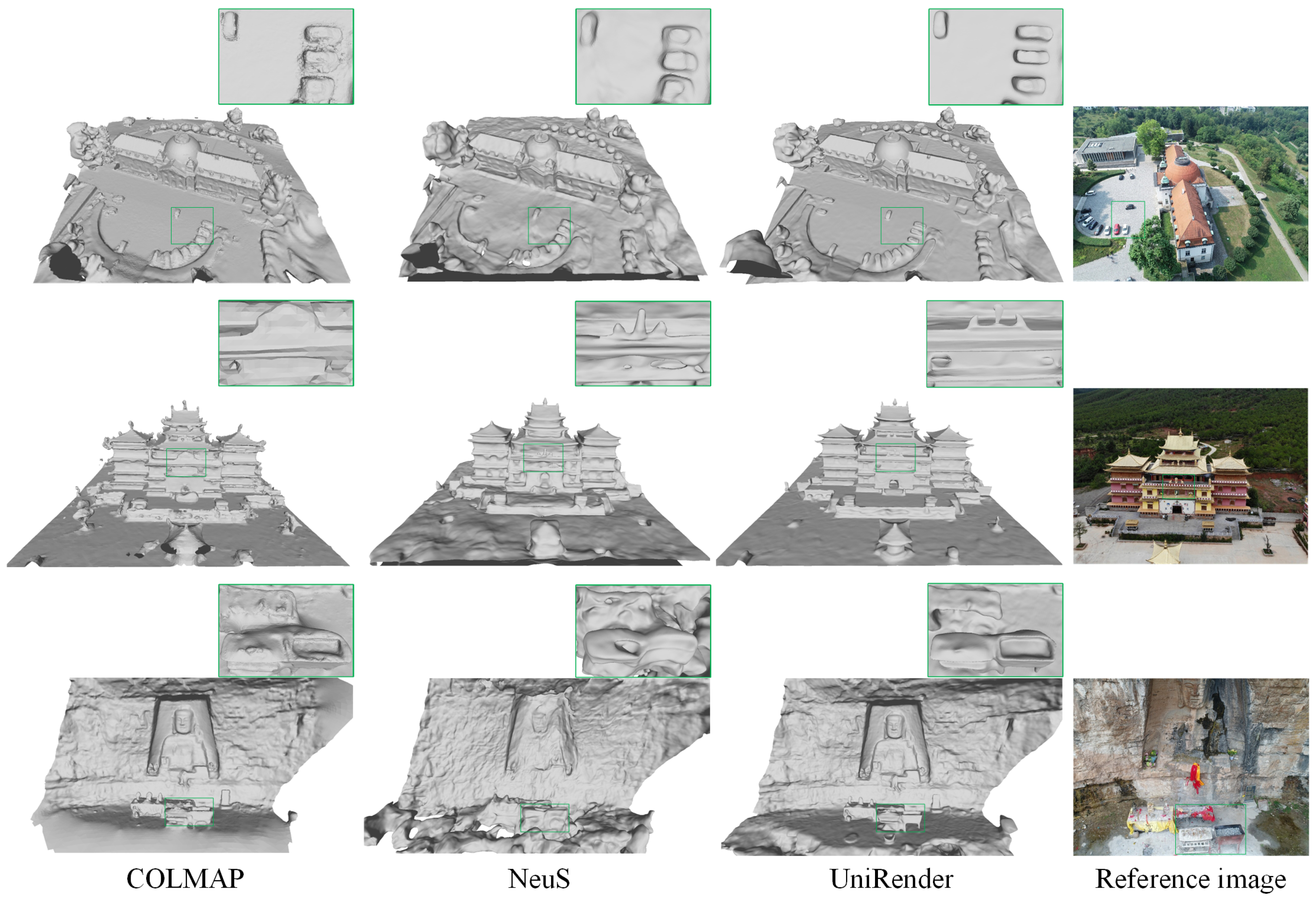
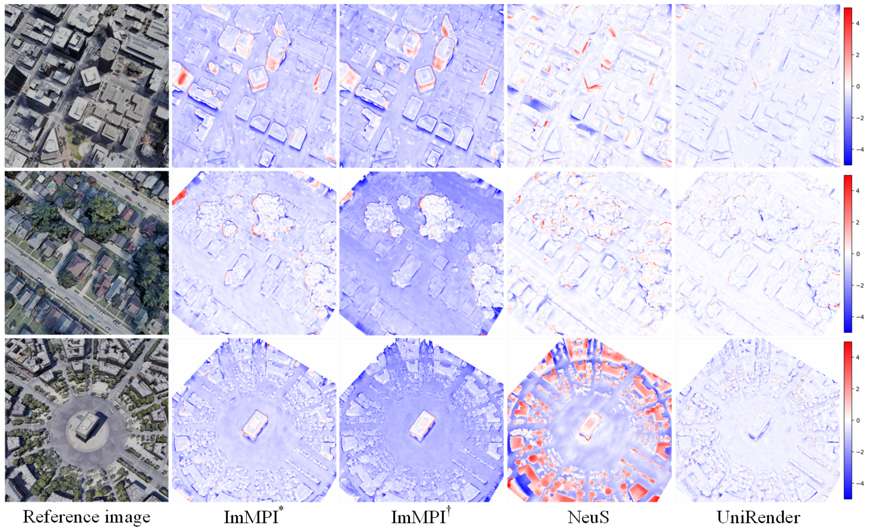
  • Color bias: Given a ray, volume rendering directly optimizes the color integration along the ray rather than the surface color where the ray intersects the surface; therefore, the estimated color at the surface, i.e., the surface-rendered color, may deviate from the volume-rendered color. We note this color bias phenomenon is particularly evident in remote sensing scenes, as shown in Figure 1 (2nd row, 2nd column and 3rd column). For methods that rely on color to optimize geometry, color bias will inevitably erode their geometric constraint ability.
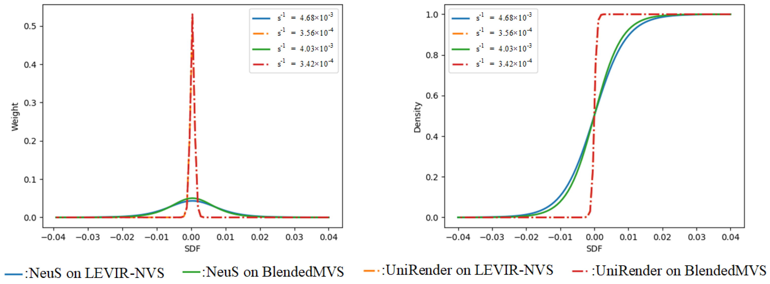
  • Weight bias: Take the volume rendering method NeuS [13], as an example. This assumes that when approaching the surface along the ray, the weight distribution of color used to compute the color integration will reach its maximum at the position of the zero signed distance field (SDF) value, i.e., the surface position, as shown in Figure 1 (1st row, 2nd column). This assumption often holds for datasets with close-up dense views and simple geometry, such as a DTU dataset [22]. However, things are different on remote sensing datasets, in which the position with the maximum weight value usually deviates from the position with the zero SDF value, as shown in Figure 1 (2nd row, 2nd column). Such a weight bias phenomenon results in a misalignment between color and geometry, and prevents volume rendering from capturing the correct geometry.
  • Geometric ambiguity: For most neural rendering pipelines [11,12,13,14], the geometry is only constrained by the color loss from a single view in each iteration, which cannot guarantee consistency across different views in the direction of geometric optimization, thus leading to ambiguity. When the input views become sparse, this ambiguity increases and results in inaccurate geometry. For remote sensing scenes, in which views are often sparse, this inherent ambiguity is undoubtedly a challenging issue.
Therefore, we aimed for a method that could incorporate both the unbiased characteristic of surface rendering and the long-distance spatial receptive field of volume rendering. UNISURF [18] has attempted to unify these two rendering methods. Its strategy is to first take a coarse sampling and to estimate surface points from the sampling points, via root-finding; it then takes a fine sampling around these surface points and performs volume rendering. The sampling interval k is controlled by the formula: k = m a x ( m a x e x p ( k , β ) , m i n ) , where k denotes the iteration number, β , and where m a x and m i n are predefined hyperparameters. However, this manner of setting a sampling interval manually is less robust. Therefore, we propose our solution. In brief, our solution is different from UNISURF [18], as follows:
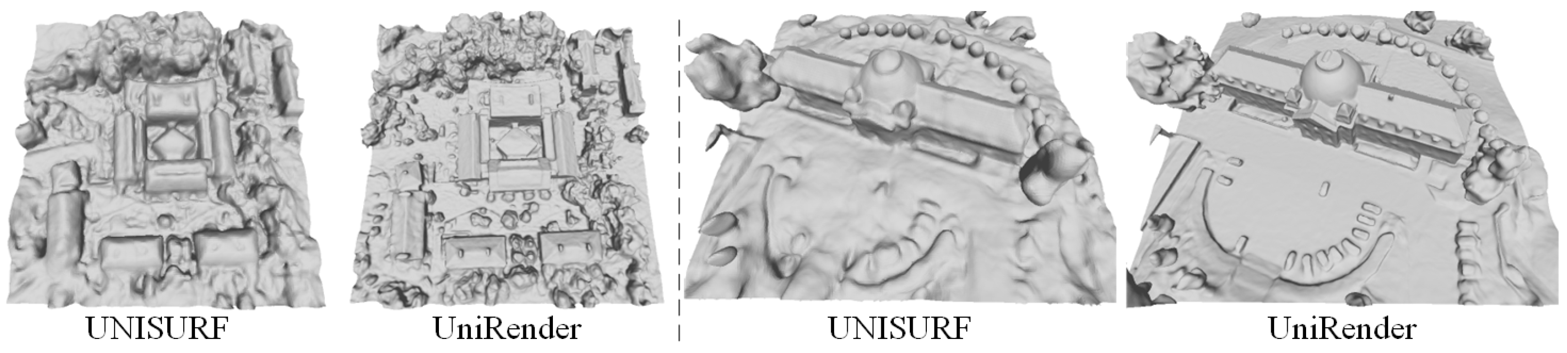
  • UNISURF [18] represents the scene geometry by occupancy values, while we use SDF representation and, thus, produce a higher-quality surface.
  • UNISURF [18] makes a transition from volume rendering to surface rendering by gradually narrowing the sampling intervals during optimization. But the sampling interval is manually defined and controlled by hyperparameters, such as iteration steps, while our method spontaneously completes this transition along with the convergence process of the networks.

3. Preliminaries

Given a set of calibrated multi-view images, our goal is to reconstruct 3D surfaces of the scene. As a by-product, realistic views can also be achieved. An overview of our approach is shown in Figure 2. Since we employ an SDF function to represent the geometry of the scene, in this section we review the fundamentals of SDF-based volumetric rendering, so that we can better demonstrate our analysis in later sections.

3.1. Scene Representation

Let the set Ω R 3 represent the space occupied by objects like trees and buildings, and let S represent the boundary of the occupied space, i.e., the earth surface. We model the entire space, including occupied and unoccupied, with the signed distance field (SDF) function f, which maps a spatial position p R 3 to a scale value,
f ( p ) = ( 1 ) I Ω ( p ) min q S p q 2 , I Ω ( p ) = 1 ,   i f p Ω 0 ,   i f p Ω ,
where I Ω ( · ) is an indicator function of the space Ω . This allows the surface S of the scene to be represented by the zero-level set of function f,
S = p R 3 | f ( p ) = 0 .
In addition to geometry, the scene appearance is represented by a function c: R 3 × R 3 R 3 that maps a spatial position p R 3 and a view direction v R 3 to a color value:
c ( p , v ) = R G B .
Finally, we use the same network architecture as IDR [8], i.e., different multi-layer perceptrons (MLPs) are used to encode functions f and c. Specifically, functions f and c are encoded by MLP networks F θ and C ψ , respectively, as shown in Figure 2. This architecture facilitates the deconstruction of geometry and appearance.

3.2. Paradigm of Volume Rendering

Given a pixel and a camera position o , we denote the ray emitted by the camera and passing through the pixel as p ( t ) = o + t v ,   t 0 , where v is the unit direction vector of the ray and t is the depth along the ray starting at o . With volume rendering, the color observed at the pixel along the direction v can be estimated by color integration,
C ( o , v ) = 0 w ( t ) c ( t ) d t ,
where c ( t ) = c ( p ( t ) , v ) is the color estimated by function c at point p ( t ) along the view direction v , and w ( t ) = w ( p ( t ) ) is the color weight at point p ( t ) along the ray. And w ( t ) is computed by the standard volume rendering Formula ([21]),
w ( t ) = T ( t ) σ ( t )
T ( t ) = exp ( 0 t σ ( u ) d u ) ,
where σ ( t ) = σ ( p ( t ) ) is the volume density at point p ( t ) , and where T ( t ) is the so-called accumulated transmittance along the ray. For simplicity, we ignore intermediate variables, and we write c , w , σ as functions of t.

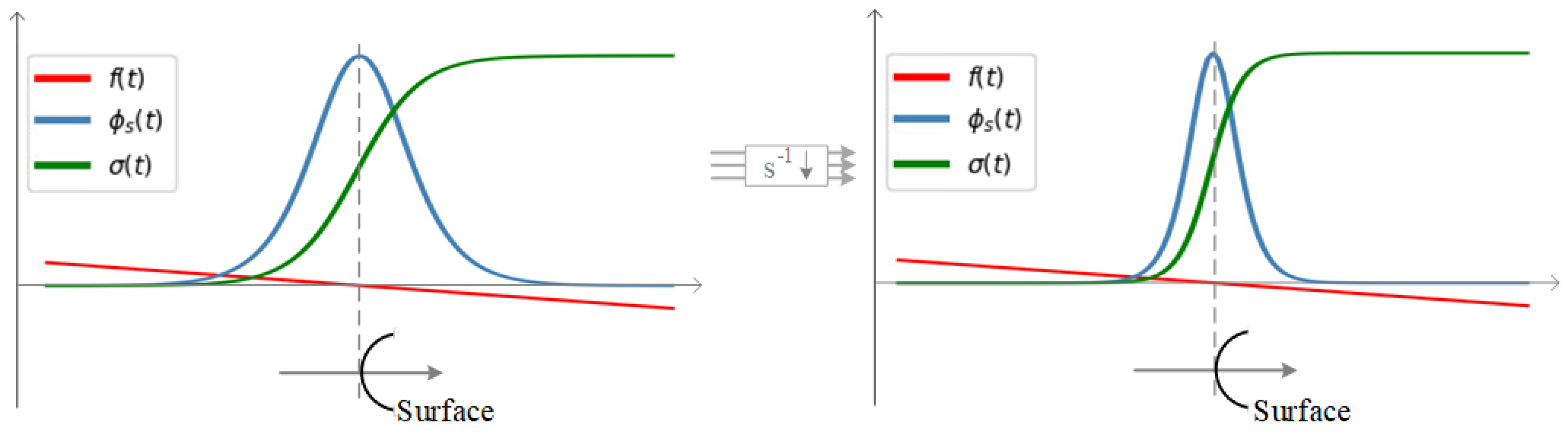
3.3. SDF-Induced Volume Density
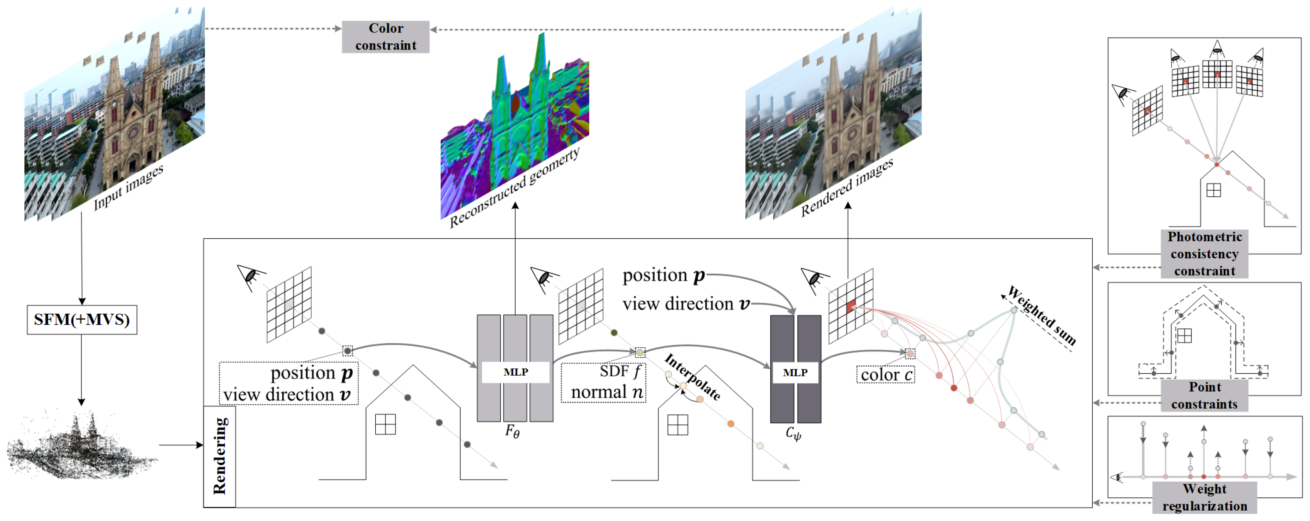
To capture the SDF representation of the scene geometry via volume rendering, it is necessary to build an appropriate connection between the SDF value f ( t ) and the volume density σ ( t ) . We employ the same strategy as NeuS [13], i.e., deriving the volume density σ from the SDF via
σ ( t ) = ψ ( f ( p ) ) = max ( ϕ s ( f ( p ( t ) ) ) Φ s ( f ( p ( t ) ) ) , 0 ) ,
where Φ s ( x ) = ( 1 + e s x ) 1 is a Sigmoid function, and ϕ s ( x ) = ( s e s x ) / ( 1 + e s x ) 2 is a logistic density distribution and also the derivative of Φ s ( x ) , while s 1 is a trainable standard deviation that should tend to zero as the networks converge.
In Figure 3, we illustrate the relationship between the SDF value f ( t ) , the volume density σ ( t ) , and ϕ s ( t ) when the ray intersects a single plane. It can be seen that as parameter s 1 decreases, the gradient of the volume density near the surface steepens, and ϕ s ( x ) contracts towards zero. Since color weight w ( t ) differs only by a factor from ϕ s ( t ) , i.e., w ( t ) = c o s θ ϕ s ( t ) , reducing s 1 leads to a more concentrated distribution of the color weight near the surface, where θ is the angle between the ray and the surface.

4. Method

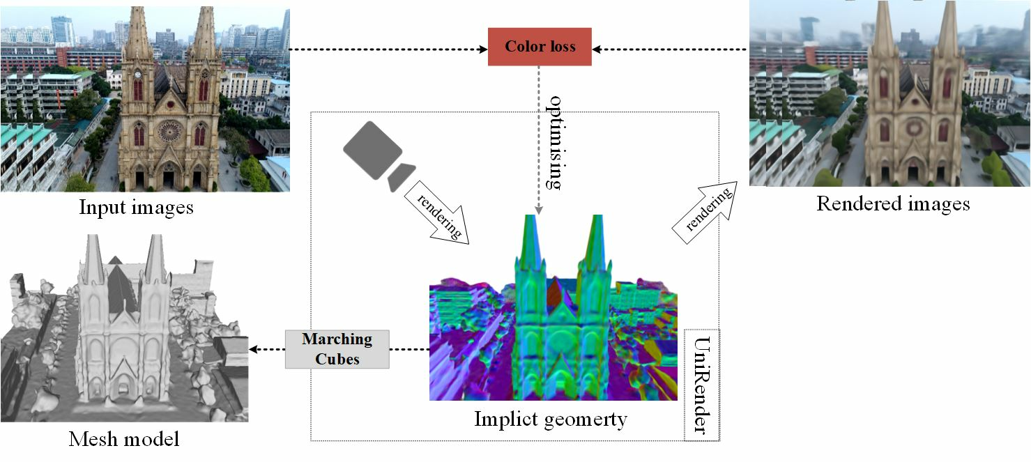
4.1. Unified Rendering Scheme

As mentioned in Section 2.3, biases in volume rendering will lead to inaccurate geometry. Let us briefly analyze these biases, before describing our solution in detail. Given the sampling points P = p ( t i ) | t n t i t f , i 1 , 2 , n sampled along the ray p ( t ) that is passing through a pixel, and the corresponding depth range of the sampling [ t n e a r , t f a r ] , the volume-rendered color of the pixel can be achieved by the discrete counterpart of Formula (4):
C v o l u m e = C ( o , v ) = i = 1 n w ( t i ) c ( t i ) .
We assume that the first intersection point of the ray and the surface is p ( t * ) , i.e., f ( p ( t * ) ) = 0 . Then, the surface color at p ( t * ) along the direction v , i.e., the surface rendering color can be expressed as
C s u f a c e = c ( t * ) .
With Formulas (8) and (9), the color bias between the volume-rendered color and the surface color can be derived as
c = C v o l u m e C s u r f a c e = i = 1 i j n w ( t i ) c ( t i ) + w ( t j ) c ( t j ) c ( t * ) = i = 1 i j n w ( t i ) c ( t i ) + ( w ( t j ) 1 ) c ( t j ) + c ( t j ) c ( t * ) = w e i g h t + c ( t j ) c ( t * ) = w e i g h t + d i s c .
This formula indicates that the color bias c can be interpreted as the sum of w e i g h t and d i s c . Where w e i g h t is the weight bias mentioned in Section 2.3 and is caused by an unreasonable weight distribution, d i s c is a bias introduced by discrete sampling, t j is the depth of the point p ( t j ) , and p ( t j ) is the point closest to the surface point p ( t * ) in the point set P .
To eliminate these biases, we propose a novel rendering scheme that unifies volume rendering and surface rendering. Specifically, we achieve this through (1) interpolated volume rendering, (2) weight regularization, and (3) unified color constraints.

4.1.1. Interpolated Volume Rendering

To eliminate d i s c , we first start with the camera position o and move along the direction v . While moving, we find the first pair of adjacent sampling points that satisfies the condition
f ( p ( t i ) ) f ( p ( t i + 1 ) < 0 ,
and we denote them as p ( t j ) and p ( t j + 1 ) , which means the two adjacent sampling points closest to the surface. Given p ( t j ) and p ( t j + 1 ) , the first intersection point of the ray and the surface p ( t * ) can be approximated as p ( t * ^ ) by linear interpolation:
p ( t * ^ ) = 0 + t * t * = f ( p ( j ) ) t j + 1 f ( p ( t j + 1 ) ) t j f ( p ( t j ) ) t j + 1 f ( p ( t j + 1 ) ) t j .
Subsequently, we add the point p ( t * ^ ) to the point set P , to obtain a new point set P = P p ( t * ) , and we use P to produce the final volume rendering color:
C v o l u m e = C ( o , v ) = i = 0 n w ( t i ) c ( t i ) + w ( t * ^ ) c ( t * ^ ) .
As C ( t , v ) is updated to C ( t , v ) , c will also be updated to
c = C v o l u m e C s u r f a c e = i = 1 n w ( t i ) c ( t i ) + w ( t * ^ ) c ( t * ) c ( t * ) = i = 1 n w ( t i ) c ( t i ) + ( w ( t * ^ ) 1 ) c ( t * ) + c ( t * ^ ) c ( t * ) = w e i g h t + c ( t * ^ ) c ( t * ) = w e i g h t + i n t e r p .
This formula indicates that w e i g h t and d i s c are updated to w e i g h t and i n t e r p , respectively, after interpolation, where i n t e r p is a bias caused by linear interpolation and is at least two orders of magnitude smaller than d i s c .

4.1.2. Weight Regularization

To alleviate the updated weight bias w e i g h t , we propose L w e i g h t , to regularize the weight distribution:
L w e i g h t = i = 1 n w ( t i ) t i t * .
L w e i g h t aims to penalize anomalous weight distributions, such as those that are far from the surface but have large weight values, thus indirectly driving the weight distribution to shrink towards the surface. Theoretically, as w ( t ) tends to δ ( t t * ^ ) , a delta distribution centered at t * ^ , w e i g h t will tend to zero, and volume rendering will produce the same result as surface rendering.
Incidentally, Mip-NeRF 360 [31] employs a regularization loss function called L d i s t , which is similar to L w e i g h t . However, L d i s t is calculated by a double integration. For a ray with n sampling points, L d i s t ’s time complexity is O ( n 2 ) , while L w e i g h t ’s is O ( n ) .

4.1.3. Color Constraints

With C v o l u m e , the color loss of volume rendering can be defined as
L v o l = C v o l u m e C G T ,
where C G T is the true color value at the pixel through which the ray p ( t ) passes.
Based on previous interpolation operations, the surface-rendered color is readily available, i.e., C s u r f a c e = c ( t * ) . We use it to produce another color loss:
L s u r f = C s u r f a c e C G T .
In fact, L s u r f not only optimizes the color at the surface, but also implicitly includes the constraint i = 1 n w ( t i ) > 0 .
Ultimately, the color loss of our framework is defined as
L c o l o r = L s u r f + L v o l .

4.2. Geometric Constraints

To alleviate the geometric ambiguity described in Section 2.3, we introduce (1) photometric consistency constraints [27], and (2) point constraints, to supervise the learned scene geometry on the SDF representation.

4.2.1. Photometric Consistency Constraints

Let the view to be rendered be the reference view I r , and let its neighboring views be the source views I i | i 1 , , m . If the ray p ( t ) and the pixel I r ( x ) in the reference view it passes through are given, we can find the surface intersection point p ( t * ^ ) , as described in Section 4.1.1. And, once p ( t * ^ ) is found, its projections in the source views I i ( x i ) | i 1 , , m can be located by a homography matrix H i ,
x i = H i x H i = K i ( R i R r T R i ( R i T t i R r T t r ) n T d ) K r 1 ,
where K r and K i , and R r and R i , and t i and t r are the internal calibration matrices, rotation matrices, and the translation vectors of the views I r and I i , respectively. Note that n and d come from the plane tangent to the surface at the point p ( t * ^ ) :
n T p ( t * ^ ) + d = 0 .
Formula (19) actually describes the relationship between the projections of point p ( t * ^ ) in different views. In addition, this relation can be extended to pixel patches. If X and X i are the patches centered at x and x i , respectively, then we have X i = H i X .
Intuitively, if p ( t * ^ ) is indeed a surface point, then its projections in different views should be consistent. Therefore, we construct a loss function, to supervise the surface we find by measuring the photometric consistency between X and X i .
Specifically, we use normalization cross-correlation as the photometric consistency metric between patches, and this can be computed by
N C C ( X , H i X ) = C o v ( X , H i X ) V a r ( X , H i X ) ,
where C o v and V a r denote covariance and variance, respectively. To deal with occlusions, the 4 best N C C scores in N C C ( X , H i X ) | i 1 , , m are selected, for calculating the final photometric consistency loss [24]:
L p h o t o = i = 1 4 1 N C C ( X , H i X ) 4 .

4.2.2. Point Constraints

Consider that current neural rendering pipelines require images with known camera poses that are typically estimated from structure-from-motion (SFM) [5]. Actually, SFM also reconstructs sparse 3D points. Although these points inevitably suffer some noise, they still have some accuracy. Meanwhile, since we are using an end-to-end framework, the noise can be corrected, to a certain extent, during optimization. Therefore, we use these reconstructed points p r e c to supervise f directly. For those scenes with sparse input views, e.g., the LEVIR-NVS scenes described by 21 images, since the time cost of executing MVS is cheap and can be limited to 10 min, we proceed to execute MVS [6] and use its reconstructed points as p r e c :
L S D F = p p r e c 1 N f ( p ) ,
where N is the number of points that p r e c contains. If we assume that any point p in p r e c is on the real surface, and that the SDF function f does capture the surface correctly, then f should satisfy f ( p ) = 0 , p p r e c . Therefore, L S D F encourages f to fit the coordinate distribution of p r e c .
Because the points generated by MVS [6] are oriented, we regard the normals of these points as additional geometric clues, and we use them to constrain the predicted normals computed with automatic differentiation on function f:
L n o r m = p p r e c 1 N p ( f ( p ) ) p ( f ( p ) ) 2 n ( p ) .

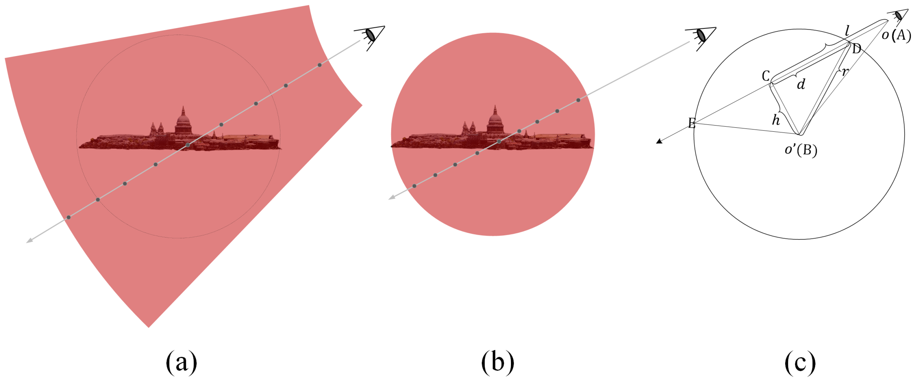
4.3. Spherical Sampling

Because many BlendedMVS scenes contain a lot of background information (such as the sky), modeling the background is necessary. As NeRF++ [32] did, we divide the scene space into an inner-sphere space and an outer space. The inner-sphere space is responsible for modeling the foreground and it is represented by the functions of f and c described in Section 3.1, while the outer space is responsible for modeling the background, and it is represented by a density-based neural field.
When sampling points, previous works first sampled in a sector space and then assigned the sampling points in the inner-sphere space to the function f, and the rest to the density-based neural field. Since the number of sampling points on each ray is fixed, this approach actually reduces the sampling points in the inner space and increases the sampling points in the outer space. This goes against our intention of allocating the main attention to the foreground, because we are primarily concerned with the quality of the surface reconstruction in the inner space. Therefore, we propose to sample directly in the inner space, as shown in Figure 4b. Specifically, we achieve this by finding the depths of the intersections where the ray enters and exits the inner space, as shown in Algorithm 1 and Figure 4c.
Algorithm 1: Spherical sampling algorithm
Input: the camera position o , i.e., the starting point of the ray
   the view direction v along the ray
   the spatial origin position o
   the radius of the inner space r
Output: the depth range to sample along the ray [ t n , t f ]
 1: Calculate the projection length of the vector o o in the ray direction: l = ( o o ) v .
 2: Calculate the length of the right-side BC of the right triangle △ABC: h = ( r 2 l 2 ) 1 / 2 .
 3: Calculate the length of the right-side CD of the right triangle △ABC: d = ( r 2 h 2 ) 1 / 2 .
 4: Determine the sampling range along the ray [ t n , t f ] : t n = l d , t f = l + d .

Implementation Details

Similar to [8,13], the functions of f and c are encoded by an 8-layer and a 4-layer MLP with 256 hidden units, respectively, while the function r is encoded by the same network structure as [8]. We sample 2048 rays per batch. For each ray, we first sample 32 points uniformly and then sample 96 points hierarchically. We train our model for 50k iterations with about 5 h on a single NVIDIA RTX3090 GPU.
The overall loss we use during training is defined as
L = L c o l o r + α L w e i g h t + β L p h o t o + L S D F + γ L n o r m + λ L E ,
where L E is the Eikonal regularization [33] for regularizing the gradients of the SDF function. In our experiments, we empirically set α = 0.1 , β = 0.2 , and γ = λ = 0.1 , to control the contribution of each loss to the error gradient. The patch size used to compute L p h o t o was 5 × 5 , which was smaller than the patch size of 11 × 11 used in most methods, since we found that using a large patch size might cause occlusions in remote sensing scenes.
After training, we use the marching cube algorithm [34] at 512 3 resolution, to extract a triangular mesh from the function f.

5. Experiments

5.1. Exp Setting

5.1.1. Dataset

Our method was evaluated on two datasets: BlendedMVS and LEVIR-NVS. Views of these two datasets are shown in Figure 5.
The BlendedMVS [35] dataset is a large-scale dataset designed to evaluate the performance of 3D reconstruction algorithms. We selected eight scenes captured in UAV view from the low-resolution BlendedMVS dataset, to test our method. The number of images in each scene ranged from 75 to 472, and the resolution of each image was 768 × 576.
The LEVIR-NVS [20] dataset includes 16 remote sensing scenes, and its views resemble satellite views that are taken from high angles. We evaluated our method’s performance on all scenes; each scene contained only 21 RGB images with a resolution of 512 × 512 pixels, thus leading to a limited range of visual field variations.

5.1.2. Baseline

Three typical scene reconstruction solutions were compared to our approach, including the traditional MVS method, COLMAP [6], the neural-volume-rendering-based method, NeuS [13], and the neural-multiplanar-representation-based method, ImMPI [20].
For COLMAP [6], the parameter trim was set to zero, when reconstructing the meshes.
For NeuS [13], we also sampled 2048 rays per batch, and we set the number of iterations to 50k, while leaving other settings unchanged.
For ImMPI [20], we only evaluated its performance on the LEVIR-NVS dataset, because it does not consider the problem of handling scenes that contain background elements, such as sky and vistas, which are common in the BlendedMVS dataset. Additionally, we used two versions of ImMPI [20] during comparison. One version, denoted as ’ImMPI * ’, was first pre-trained on WHU [36] and then trained with 11 views. The other version, denoted as ’ImMPI ’, was not pre-trained, but was trained using all 21 images.

5.1.3. Evaluation Metrics

Similar to MVSNet [37], we evaluated the surface reconstruction performance by both the distance metric [22] and the percentage metric [38]. Assuming that S 1 represented the ground truth points and that S 2 represented the points sampled from the reconstructed surface, the chamfer distance from S 1 to S 2 was considered as the evaluation metric for reconstruction accuracy (Acc):
Acc = d C D ( S 1 , S 2 ) = 1 S 1 x S 1 min y S 2 x y 2 .
The charmful distance from S 2 to S 1 was considered as the evaluation metric for reconstruction completeness (Comp):
Comp = d C D ( S 2 , S 1 ) = 1 S 2 x S 2 min y S 1 x y 2 .
The overall score was defined as the mean of accuracy and completeness. The percentage metric measured accuracy and completeness in a similar manner, by introducing a distance threshold, and it evaluated the overall performance by F-score.

5.2. Results

We first compared the surface reconstruction results on BlendedMVS, which are shown in Figure 6 and Table 1. It can be observed that the reconstructed surfaces from COLMAP [6] were noisy, while NeuS [13] struggled with capturing accurate geometric structures using only color constraints. By contrast, UniRender achieved a balance between precise geometry and smooth surfaces.
Then, we performed similar experiments on the LEVIR-NVS dataset, and the results are shown in Figure 7 and Table 2. In contrast to the BlendedMVS dataset, the scenes in LEVIR-NVS had sparse views, which caused a relative decline in COLMAP [6]’s performance, particularly in marginal regions. NeuS [13] seemed to adapt better to the LEVIR-NVS dataset, but it performed poorly in near-ground regions.
We also show the depth estimation results on the LEVIR-NVS dataset in Table 3 and Figure 8, in which the mean absolute error (MAE) was used as the evaluation metric. It can be seen that both imMPI * and imMPI had a large MAE, but that the imMPI without pre-training had the largest MAE. NeuS struggled with scenes, such as the square. And, except for Unirender, all the methods had difficulty estimating accurate depth information for the facades of high-rise buildings.
Given that UNISURF [18] is a work similar to UniRender, we further compared the 3D reconstruction results between them. As illustrated in Table 4 and Figure 9, it was evident that UNISURF [18] significantly lagged behind UniRender, in both numerical metrics and visualization.

5.3. Discussion

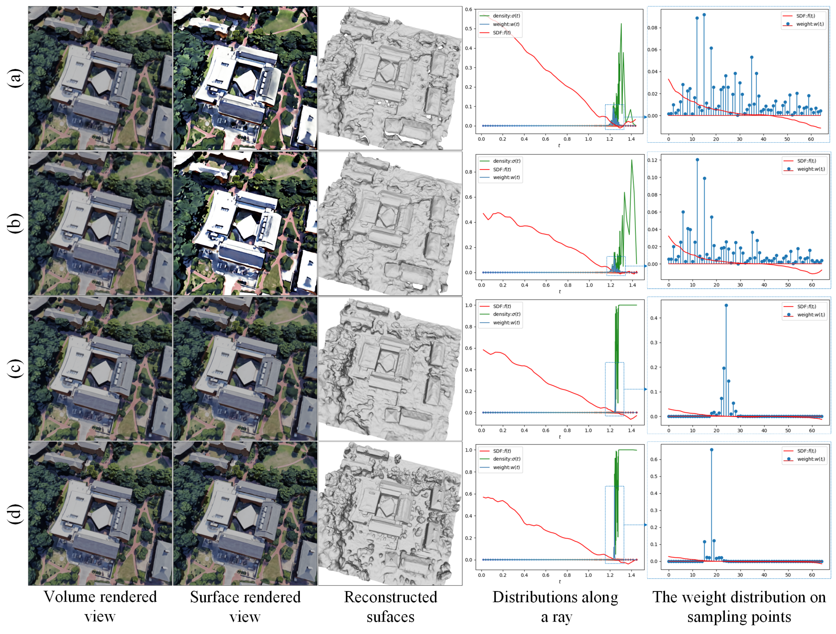
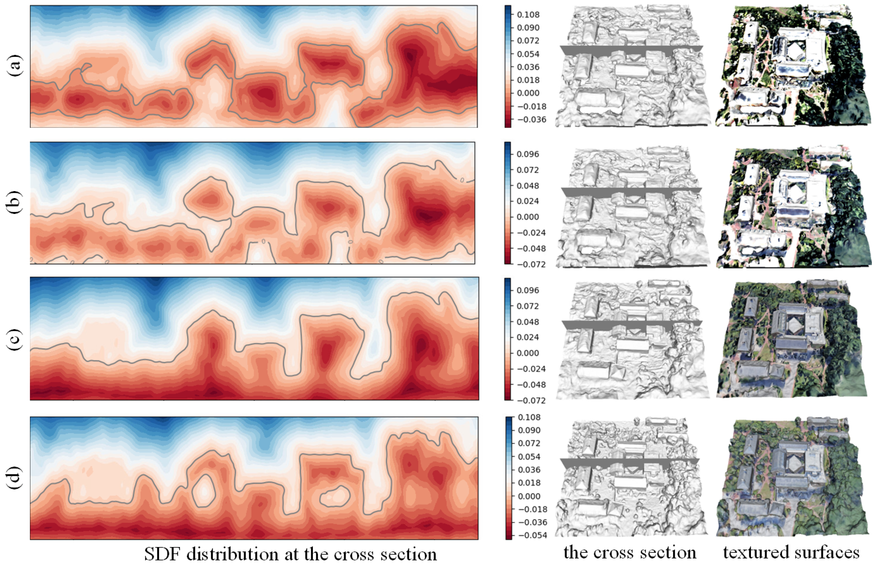
5.3.1. Biases Elimination Verification

To study the effectiveness of our method for bias elimination, we used NeuS [13] as the baseline, and we conducted experiments on the LEVIR-NVS dataset with different settings:
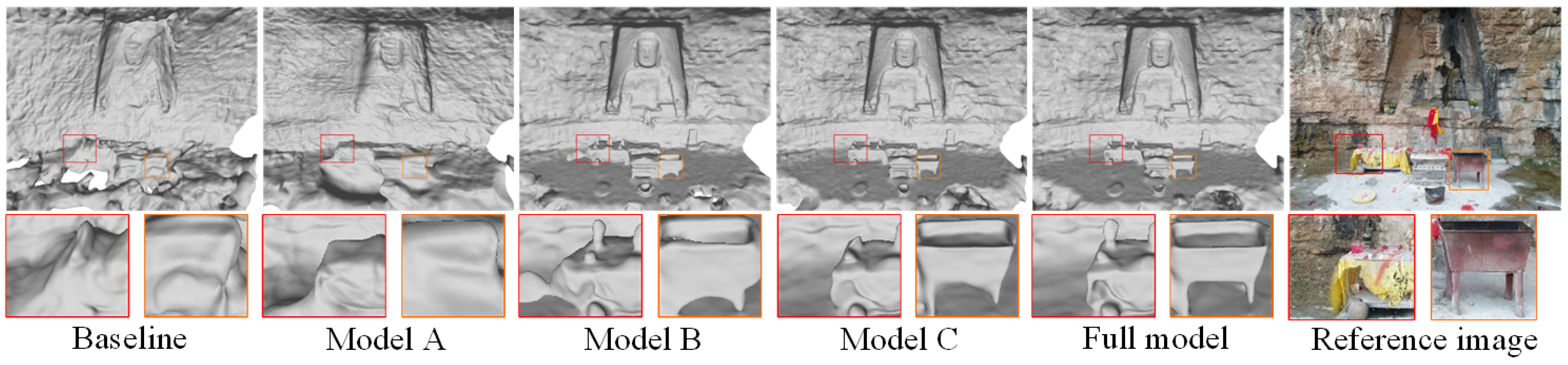
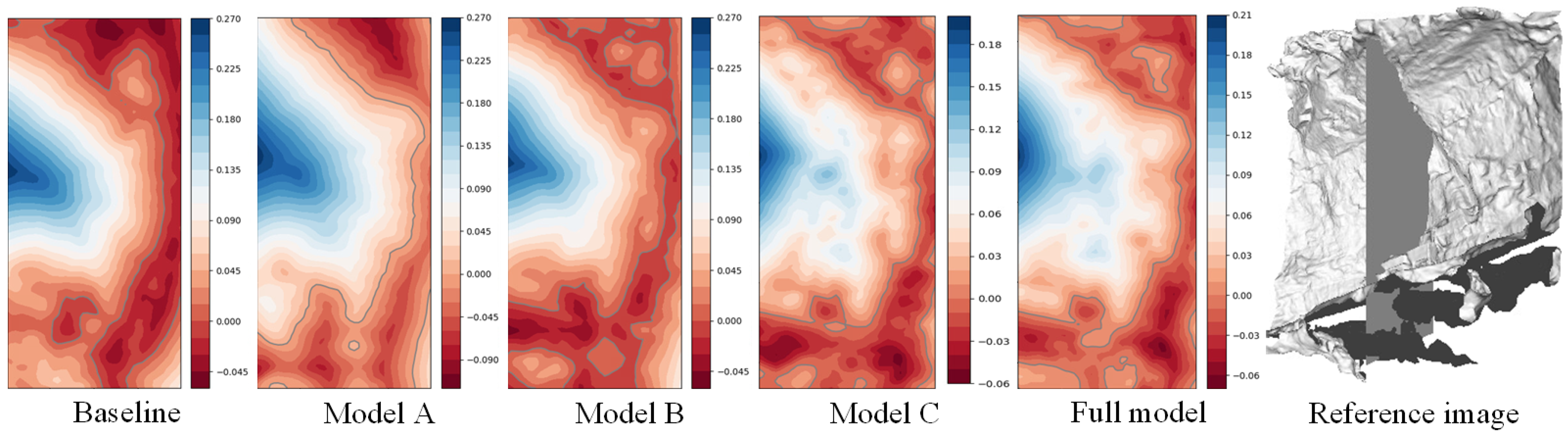
  • (a) using a sampling strategy that first sampled 64 points uniformly and then sampled 64 points hierarchically.
  • (b) using a sampling strategy that first sampled 32 points uniformly and then sampled 96 points hierarchically.
  • (c) replacing the rendering scheme of NeuS [13] with our proposed rendering scheme, and using the same sampling strategy as (b).
  • (d) adding all the geometric constraints based on (c).
As the results show in Figure 10, (a) unsurprisingly produced obvious color bias and weight bias during rendering, and outputted a low quality surface with many holes, while (b) showed that simply changing the sampling strategy did not help eliminate biases and that the reconstructed surface remained poor. Gratifyingly, with the unbiased rendering scheme, (c) significantly reduced the biases, while the holes in the reconstructed surface were filled, and buildings’ outlines were improved. Finally, with the geometric constraints, (d) further tended the weight distribution to a delta function, and details such as shrubs were shown on the reconstructed surface.
We also show the SDF distribution and textured surfaces with settings (a,d) in Figure 11. Comparing (a,b) and (c,d), it can be seen that the proposed rendering scheme not only produces reasonable colors at surfaces, but also facilitates the fitting of the SDF distribution to the remote sensing scenes. Because of the remote sensing scenes, we wish the SDF distribution to have only one zero value in the vertical direction.

5.3.2. Optimization of the Parameters s 1

As described in Section 3.3, s 1 is a trainable parameter, which controls the slope of the density distribution near the surface and also is the standard deviation of the weighting distribution. In addition, it reflects how well the networks fit a scene. When training is complete, the smaller the parameter, the steeper the slope of the density function around the surface, and the more the weight distribution tends towards a delta distribution. This indicates that the network fits the scene better. Figure 12 illustrates the degree to which NeuS [13] and UniRender are optimized for parameter s 1 .

5.3.3. Ablation Study

To evaluate the effectiveness of the individual modules that we propose, we conducted further ablation studies on the BlendedMVS dataset. We adapted NeuS [13] as the baseline, and we selectively added these modules to it. As shown in Figure 13, the baseline produced severely distorted geometric surfaces with large holes. Model A produced smooth and continuous surfaces, but only approximated the real geometry. Model B showed an effective enhancement to the geometric quality, but it also produced redundant surfaces and holes. Model C yielded a reconstructed surface with no obvious geometric errors. However, Model D provided a more detailed result. In summary:
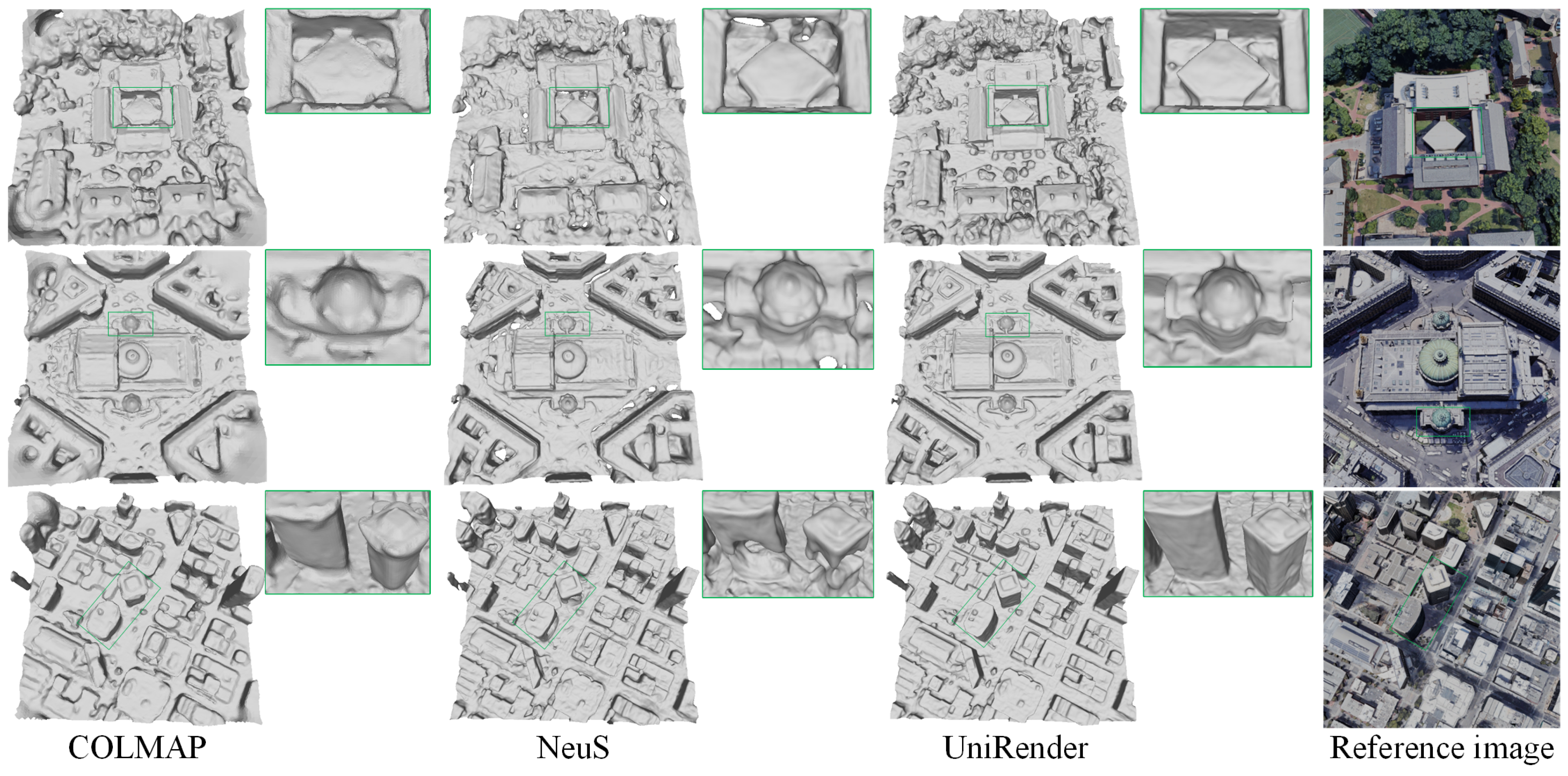
  • The unified rendering scheme tends to produce smooth and continuous surfaces, and improves geometric accuracy to some extent.
  • The geometric constraint mechanisms are effective in improving the quality of geometric reconstruction.
  • The spherical sampling strategy can facilitate the capture of detail.
One point worth noting is that although Mode A was optimal, in terms of the numerical results in Table 5, its visualization results were not as good. A reasonable explanation for this contradiction is that there were plenty of redundant surfaces located on the back of the visible surfaces in all cases, except for Model A, as shown in Figure 14. The redundant surfaces severely reduced the Acc value for all the models, except Model A, while Model A produced a relatively clean surface, thus resulting in a lower overall value.

6. Conclusions and Outlook

6.1. Conclusions

We present UniRender, a novel 3D surface reconstruction method with neural rendering. In this work, we first analyzed the biases in current volume rendering methods, and we developed an approximately bias-free rendering scheme that unifies volume rendering and surface rendering through a natural transition. Then, we introduced several multi-view geometric constraints into the rendering pipeline, to improve its ability for capturing accurate geometry. Finally, a spherical sampling algorithm was proposed, for allocating more attention to the space with which we were concerned. Extensive experiments on different remote sensing datasets showed that UniRender outperforms other types of 3D surface reconstruction methods by a wide margin.
The main significance of this work is that it identifies the biases that exist in the current volume rendering branch and it proposes a unified rendering strategy to address them. This rendering strategy can be seamlessly integrated into other 3D rendering frameworks, offering universal applicability. Additionally, this work introduces new ideas for jointly optimizing multi-view geometric constraints within neural rendering. Finally, extensive experiments demonstrated the effectiveness of the proposed method and they also promoted the application of neural rendering in remote sensing.

6.2. Outlook

Similar to other neural rendering methods, it takes several hours to train our model for each scene. This is because forward inference and backpropagation for each spatial coordinate point by MLPs consume a significant amount of computational power. Some recent advancements in computer vision have tried to expedite the rendering process, through voxel-based architecture [39,40]. Although these techniques were not originally designed for 3D reconstruction and remote sensing scenarios, they hold significant promise of alleviating the current time-consuming challenges.
Moreover, UniRender currently does not have the ability to perform large-scale surface reconstruction. This is because the fidelity of scene reproduction by MLPs with finite parameters decreases as the scene’s scale increases. This is akin to representing a scene with a fixed-size image, where larger scenes result in lower spatial resolution images. Therefore, constructing neural rendering models for large-scale scenes remains a significant challenge. Fortunately, recent approaches, like Mega-NeRF [41] and Block-NeRF [42], have suggested a potential solution: partitioning a large scene into multiple sub-blocks and employing multiple models to process these sub-blocks in parallel.
In summary, building a faster framework with large-scale processing capability is our future endeavor.

Author Contributions

Conceptualization, Y.Y. and N.S.; methodology, Y.Y. and W.Z.; software, W.Z.; validation, Y.Y. and C.Z.; formal analysis, Y.Y. and C.Z.; resources, Y.Y. and N.S.; data curation, W.Z.; writing—original draft preparation, Y.Y. and W.Z.; writing—review and editing, Y.Y., W.Z. and C.Z.; supervision, Y.Y. and N.S.; funding acquisition, Y.Y. and N.S. All authors have read and agreed to the published version of the manuscript.

Funding

This research was funded by the National Natural Science Foundation of China (No. 62071136, No. 62271159) and the Heilongjiang Outstanding Youth Foundation (YQ2022F002).

Data Availability Statement

The data used in this study are publicly available at https://github.com/SunshineWYC/ImMPI and https://github.com/YoYo000/BlendedMVS, accessed on 16 September 2023.

Acknowledgments

Thanks to the excellent works of [6,13,20,24,35,37], we utilized some of their code implementations and datasets to support our research.

Conflicts of Interest

The authors declare no conflict of interest.

Appendix A

Figure A1. The scenes in the Blended MVS dataset that we used in our work, from left to right and from top to bottom, are scene1 to scene8, respectively. The visualization of the camera position can be found in the main text, in Table 5.
Remotesensing 15 04634 g0a1
Figure A2. All the scenes in the LEVIR-NVS dataset, from left to right and from top to bottom, are scene00 to scene15, respectively. The visualization of the camera position can be found in the main text, in Table 5.
Remotesensing 15 04634 g0a2
Table A1. Quantitative surface reconstruction results on the BlendedMVS dataset. A summary of this table is shown in the main text, in Table 1.
SceneDistance
COLMAPNeuSUniRender
Acc↓Comp↓Overall↓Acc↓Comp↓Overall↓Acc↓Comp↓Overall↓
scene1, 5bf18642c50e6f7f8bdbd4920.20870.27630.24250.27650.22070.24860.17510.10460.1398
scene2, 58eaf1513353456af3a1682a0.22810.58600.40710.29330.26130.27730.19750.12520.1613
scene3, 5b558a928bbfb62204e77ba20.25810.30270.28040.52620.51680.52150.24270.20860.2256
scene4, 5b6eff8b67b396324c5b26720.17460.64200.40830.30490.26080.28290.12760.07080.0992
scene5, 58c4bb4f4a69c55606122be40.09510.00200.04850.19950.01140.10550.10150.00150.0515
scene6, 5bd43b4ba6b28b1ee86b92dd0.09960.02670.06310.00440.00350.00390.00310.00230.0027
scene7, 5b62647143840965efc0dbde0.22000.15990.18990.54610.52570.53590.20000.12450.1623
scene8, 5ba75d79d76ffa2c86cf2f050.17390.28260.22820.52530.53930.53230.20080.14760.1742
mean0.18230.28480.23350.33450.29240.31350.15600.09810.1271
Table A2. Quantitative surface reconstruction results on the LEVIR-NVS dataset. A summary of this table is shown in the main text, in Table 2.
SceneDistance
COLMAPNeuSUniRender
Acc↓Comp↓Overall↓Acc↓Comp↓Overall↓Acc↓Comp↓Overall↓
scene00, Building#10.29000.34560.31780.50100.62880.56490.26480.32490.2948
scene01, Church0.22610.21510.22060.18590.19590.19090.16160.16660.1641
scene02, College0.30110.27220.28670.36580.35150.35870.26810.27480.2714
scene03, Mountain#10.08940.09540.09240.08220.09810.09010.09070.11230.1015
scene04, Mountain#20.08950.11510.10230.07440.09430.08430.07300.09770.0854
scene05, Observation0.25700.22180.23940.33620.28650.31140.20050.16080.1806
scene06, Building#20.28510.27840.28170.29120.25540.27330.26980.27530.2725
scene07, Town#10.23340.23680.23510.29640.22110.25880.17620.15810.1671
scene08, Stadium0.16340.15720.16030.23200.19090.21140.13770.15430.1460
scene09, Town#20.16080.17490.16790.33090.36840.34970.15390.17530.1646
scene10, Mountain#30.08350.10370.09360.07290.08850.08070.06920.08610.0776
scene11, Town#30.18180.14790.16480.16690.12480.14590.16330.14030.1518
scene12, Factory0.25660.31110.28390.39170.45970.42570.23950.29530.2674
scene13, Park0.17910.24480.21190.33560.32330.32940.19410.26280.2284
scene14, School0.18750.19100.18920.20160.21640.20900.15320.15670.1549
scene15, Downtown0.25930.27480.26710.21530.22730.22130.18350.24050.2120
mean0.21160.20270.20720.25820.25500.256640.19260.17490.1838

References

  1. Griwodz, C.; Gasparini, S.; Calvet, L.; Gurdjos, P.; Castan, F.; Maujean, B.; Lillo, G.D.; Lanthony, Y. AliceVision Meshroom: An open-source 3D reconstruction pipeline. In Proceedings of the 12th ACM Multimedia Systems Conference, Istanbul, Turkey, 28 September–1 October 2021. [Google Scholar]
  2. Rupnik, E.; Daakir, M.; Deseilligny, M.P. MicMac—A free, open-source solution for photogrammetry. Open Geospat. Data Softw. Stand. 2017, 2, 14. [Google Scholar] [CrossRef]
  3. Labatut, P.; Pons, J.P.; Keriven, R. Efficient Multi-View Reconstruction of Large-Scale Scenes using Interest Points, Delaunay Triangulation and Graph Cuts. In Proceedings of the 2007 IEEE 11th International Conference on Computer Vision, Rio de Janeiro, Brazil, 14–21 October 2007; pp. 1–8. [Google Scholar]
  4. Furukawa, Y.; Ponce, J. Accurate, Dense, and Robust Multiview Stereopsis. IEEE Trans. Pattern Anal. Mach. Intell. 2010, 32, 1362–1376. [Google Scholar] [CrossRef] [PubMed]
  5. Schönberger, J.L.; Frahm, J.M. Structure-from-Motion Revisited. In Proceedings of the 2016 IEEE Conference on Computer Vision and Pattern Recognition (CVPR), Las Vegas, NV, USA, 27–30 June 2016; pp. 4104–4113. [Google Scholar]
  6. Schönberger, J.L.; Zheng, E.; Frahm, J.M.; Pollefeys, M. Pixelwise View Selection for Unstructured Multi-View Stereo. In Proceedings of the European Conference on Computer Vision, Amsterdam, The Netherlands, 11–14 October 2016. [Google Scholar]
  7. Kazhdan, M.M.; Hoppe, H. Screened poisson surface reconstruction. ACM Trans. Graph. 2013, 32, 1–13. [Google Scholar] [CrossRef]
  8. Yariv, L.; Kasten, Y.; Moran, D.; Galun, M.; Atzmon, M.; Basri, R.; Lipman, Y. Multiview Neural Surface Reconstruction by Disentangling Geometry and Appearance. arXiv 2020, arXiv:2003.09852. [Google Scholar]
  9. Long, X.; Lin, C.H.; Wang, P.; Komura, T.; Wang, W. SparseNeuS: Fast Generalizable Neural Surface Reconstruction from Sparse views. arXiv 2022, arXiv:2206.05737. [Google Scholar]
  10. Tewari, A.; Fried, O.; Thies, J.; Sitzmann, V.; Lombardi, S.; Xu, Z.; Simon, T.; Nießner, M.; Tretschk, E.; Liu, L.; et al. Advances in Neural Rendering. Comput. Graph. Forum 2021, 41, 703–735. [Google Scholar] [CrossRef]
  11. Mar’i, R.; Facciolo, G.; Ehret, T. Sat-NeRF: Learning Multi-View Satellite Photogrammetry with Transient Objects and Shadow Modeling Using RPC Cameras. In Proceedings of the 2022 IEEE/CVF Conference on Computer Vision and Pattern Recognition Workshops (CVPRW), New Orleans, LA, USA, 19–20 June 2022; pp. 1310–1320. [Google Scholar]
  12. Derksen, D.; Izzo, D. Shadow Neural Radiance Fields for Multi-view Satellite Photogrammetry. In Proceedings of the 2021 IEEE/CVF Conference on Computer Vision and Pattern Recognition Workshops (CVPRW), Nashville, TN, USA, 19–25 June 2021; pp. 1152–1161. [Google Scholar]
  13. Wang, P.; Liu, L.; Liu, Y.; Theobalt, C.; Komura, T.; Wang, W. NeuS: Learning Neural Implicit Surfaces by Volume Rendering for Multi-view Reconstruction. In Proceedings of the Neural Information Processing Systems, Virtual, 6–14 December 2021. [Google Scholar]
  14. Yariv, L.; Gu, J.; Kasten, Y.; Lipman, Y. Volume Rendering of Neural Implicit Surfaces. arXiv 2021, arXiv:2106.12052. [Google Scholar]
  15. Zhang, J.; Yao, Y.; Quan, L. Learning Signed Distance Field for Multi-view Surface Reconstruction. In Proceedings of the 2021 IEEE/CVF International Conference on Computer Vision (ICCV), Montreal, BC, Canada, 11–17 October 2021; pp. 6505–6514. [Google Scholar]
  16. Zhang, J.; Yao, Y.; Li, S.; Fang, T.; McKinnon, D.N.R.; Tsin, Y.; Quan, L. Critical Regularizations for Neural Surface Reconstruction in the Wild. In Proceedings of the 2022 IEEE/CVF Conference on Computer Vision and Pattern Recognition (CVPR), New Orleans, LA, USA, 18–24 June 2022; pp. 6260–6269. [Google Scholar]
  17. Niemeyer, M.; Mescheder, L.M.; Oechsle, M.; Geiger, A. Differentiable Volumetric Rendering: Learning Implicit 3D Representations Without 3D Supervision. In Proceedings of the 2020 IEEE/CVF Conference on Computer Vision and Pattern Recognition (CVPR), Seattle, WA, USA, 13–19 June 2020; pp. 3501–3512. [Google Scholar]
  18. Oechsle, M.; Peng, S.; Geiger, A. UNISURF: Unifying Neural Implicit Surfaces and Radiance Fields for Multi-View Reconstruction. In Proceedings of the 2021 IEEE/CVF International Conference on Computer Vision (ICCV), Montreal, BC, Canada, 11–17 October 2021; pp. 5569–5579. [Google Scholar]
  19. Sun, J.; Chen, X.; Wang, Q.; Li, Z.; Averbuch-Elor, H.; Zhou, X.; Snavely, N. Neural 3D Reconstruction in the Wild. In ACM SIGGRAPH 2022 Conference Proceedings; Association for Computing Machinery: New York, NY, USA, 2022. [Google Scholar]
  20. Wu, Y.; Zou, Z.; Shi, Z. Remote Sensing Novel View Synthesis with Implicit Multiplane Representations. IEEE Trans. Geosci. Remote Sens. 2022, 60, 1–13. [Google Scholar] [CrossRef]
  21. Mildenhall, B.; Srinivasan, P.P.; Tancik, M.; Barron, J.T.; Ramamoorthi, R.; Ng, R. NeRF: Representing Scenes as Neural Radiance Fields for View Synthesis. arXiv 2020, arXiv:2003.08934. [Google Scholar] [CrossRef]
  22. Aanæs, H.; Jensen, R.R.; Vogiatzis, G.; Tola, E.; Dahl, A.B. Large-Scale Data for Multiple-View Stereopsis. Int. J. Comput. Vis. 2016, 120, 153–168. [Google Scholar] [CrossRef]
  23. Park, J.J.; Florence, P.R.; Straub, J.; Newcombe, R.A.; Lovegrove, S. DeepSDF: Learning Continuous Signed Distance Functions for Shape Representation. In Proceedings of the 2019 IEEE/CVF Conference on Computer Vision and Pattern Recognition (CVPR), Long Beach, CA, USA, 15–20 June 2019; pp. 165–174. [Google Scholar]
  24. Fu, Q.; Xu, Q.; Ong, Y.; Tao, W. Geo-Neus: Geometry-Consistent Neural Implicit Surfaces Learning for Multi-view Reconstruction. arXiv 2022, arXiv:2205.15848. [Google Scholar]
  25. Mescheder, L.M.; Oechsle, M.; Niemeyer, M.; Nowozin, S.; Geiger, A. Occupancy Networks: Learning 3D Reconstruction in Function Space. In Proceedings of the 2019 IEEE/CVF Conference on Computer Vision and Pattern Recognition (CVPR), Long Beach, CA, USA, 15–20 June 2019; pp. 4455–4465. [Google Scholar]
  26. Li, J.; Feng, Z.; She, Q.; Ding, H.; Wang, C.; Lee, G.H. MINE: Towards Continuous Depth MPI with NeRF for Novel View Synthesis. In Proceedings of the 2021 IEEE/CVF International Conference on Computer Vision (ICCV), Montreal, BC, Canada, 11–17 October 2021; pp. 12558–12568. [Google Scholar]
  27. Goesele, M.; Curless, B.; Seitz, S.M. Multi-View Stereo Revisited. In Proceedings of the 2006 IEEE Computer Society Conference on Computer Vision and Pattern Recognition (CVPR’06), New York, NY, USA, 17–22 June 2006; pp. 2402–2409. [Google Scholar]
  28. Barnes, C.; Shechtman, E.; Finkelstein, A.; Goldman, D.B. PatchMatch: A randomized correspondence algorithm for structural image editing. ACM Trans. Graph. 2009, 28, 24. [Google Scholar] [CrossRef]
  29. Liu, S.; Zhang, Y.; Peng, S.; Shi, B.; Pollefeys, M.; Cui, Z. DIST: Rendering Deep Implicit Signed Distance Function with Differentiable Sphere Tracing. In Proceedings of the 2020 IEEE/CVF Conference on Computer Vision and Pattern Recognition (CVPR), Seattle, WA, USA, 13–19 June 2020; pp. 2016–2025. [Google Scholar]
  30. Darmon, F.; Bascle, B.; Devaux, J.C.; Monasse, P.; Aubry, M. Improving neural implicit surfaces geometry with patch warping. In Proceedings of the 2022 IEEE/CVF Conference on Computer Vision and Pattern Recognition (CVPR), New Orleans, LA, USA, 18–24 June 2022; pp. 6250–6259. [Google Scholar]
  31. Barron, J.T.; Mildenhall, B.; Verbin, D.; Srinivasan, P.P.; Hedman, P. Mip-NeRF 360: Unbounded Anti-Aliased Neural Radiance Fields. In Proceedings of the 2022 IEEE/CVF Conference on Computer Vision and Pattern Recognition (CVPR), New Orleans, LA, USA, 18–24 June 2022; pp. 5460–5469. [Google Scholar]
  32. Zhang, K.; Riegler, G.; Snavely, N.; Koltun, V. NeRF++: Analyzing and Improving Neural Radiance Fields. arXiv 2020, arXiv:2010.07492. [Google Scholar]
  33. Gropp, A.; Yariv, L.; Haim, N.; Atzmon, M.; Lipman, Y. Implicit Geometric Regularization for Learning Shapes. In Proceedings of the International Conference on Machine Learning, Virtual, 13–18 July 2020. [Google Scholar]
  34. Lorensen, W.E.; Cline, H.E. Marching cubes: A high resolution 3D surface construction algorithm. In Proceedings of the 14th Annual Conference on Computer Graphics and Interactive Technique, Anaheim, CA, USA, 27–31 July 1987. [Google Scholar]
  35. Yao, Y.; Luo, Z.; Li, S.; Zhang, J.; Ren, Y.; Zhou, L.; Fang, T.; Quan, L. BlendedMVS: A Large-Scale Dataset for Generalized Multi-View Stereo Networks. In Proceedings of the 2020 IEEE/CVF Conference on Computer Vision and Pattern Recognition (CVPR), Seattle, WA, USA, 13–19 June 2020; pp. 1787–1796. [Google Scholar]
  36. Li, S.; He, S.F.; Jiang, S.; Jiang, W.; Zhang, L. WHU-Stereo: A Challenging Benchmark for Stereo Matching of High-Resolution Satellite Images. IEEE Trans. Geosci. Remote Sens. 2022, 61, 1–14. [Google Scholar] [CrossRef]
  37. Yao, Y.; Luo, Z.; Li, S.; Fang, T.; Quan, L. MVSNet: Depth Inference for Unstructured Multi-view Stereo. In Proceedings of the European Conference on Computer Vision, Munich, Germany, 8–14 September 2018. [Google Scholar]
  38. Knapitsch, A.; Park, J.; Zhou, Q.Y.; Koltun, V. Tanks and temples: Benchmarking large-scale scene reconstruction. ACM Trans. Graph. (TOG) 2017, 36, 1–13. [Google Scholar] [CrossRef]
  39. Sun, C.; Sun, M.; Chen, H.T. Direct Voxel Grid Optimization: Super-fast Convergence for Radiance Fields Reconstruction. In Proceedings of the 2022 IEEE/CVF Conference on Computer Vision and Pattern Recognition (CVPR), New Orleans, LA, USA, 18–24 June 2022; pp. 5449–5459. [Google Scholar]
  40. Müller, T.; Evans, A.; Schied, C.; Keller, A. Instant neural graphics primitives with a multiresolution hash encoding. ACM Trans. Graph. (TOG) 2022, 41, 1–15. [Google Scholar] [CrossRef]
  41. Turki, H.; Ramanan, D.; Satyanarayanan, M. Mega-NeRF: Scalable Construction of Large-Scale NeRFs for Virtual Fly- Throughs. In Proceedings of the 2022 IEEE/CVF Conference on Computer Vision and Pattern Recognition (CVPR), New Orleans, LA, USA, 18–24 June 2022; pp. 12912–12921. [Google Scholar]
  42. Tancik, M.; Casser, V.; Yan, X.; Pradhan, S.; Mildenhall, B.; Srinivasan, P.P.; Barron, J.T.; Kretzschmar, H. Block-NeRF: Scalable Large Scene Neural View Synthesis. In Proceedings of the 2022 IEEE/CVF Conference on Computer Vision and Pattern Recognition (CVPR), New Orleans, LA, USA, 18–24 June 2022; pp. 8238–8248. [Google Scholar]
Figure 1. An illustration of NeuS [13]’s performance on different datasets. Compared to the indoor dataset DTU [22], NeuS exhibits obvious color bias and weight bias on the remote sensing dataset LEVIR-NVS [20], while the reconstructed surfaces suffer from numerous holes and poor quality.
Remotesensing 15 04634 g001
Figure 2. An overview of UniRender. Given a ray that passes through a pixel, UniRender first samples points along the ray, then estimates the values of those points. With the SDF values, it interpolates the surface intersection point along the ray. After interpolating, it estimates the colors of all the points. Finally, a weighted sum of these colors is computed, as the estimated pixel color. During training, various constraint mechanisms are used, to optimize the MLP networks.
Remotesensing 15 04634 g002
Figure 3. An illustration of the SDF value f ( t ) , volume density σ ( t ) , and ϕ s ( t ) when the ray intersects a single plane.
Remotesensing 15 04634 g003
Figure 4. (a) The sector sampling space used by most methods, (b) the spherical sampling space that we use, (c) the illustration of Algorithm 1.
Remotesensing 15 04634 g004
Figure 5. An illustration of (a) the BlendedMVS dataset and (b) the LEVIR-NVS dataset. More details about these two datasets can be found in Appendix A Figure A1 and Figure A2. Each red dot in the figure represents a camera.
Remotesensing 15 04634 g005
Figure 6. Quantitative surface reconstruction results on the BlendedMVS dataset.
Remotesensing 15 04634 g006
Figure 7. Qualitative surface reconstruction results on the LEVIR-NVS dataset.
Remotesensing 15 04634 g007
Figure 8. Visualization of the MAE between true and estimated depth: the darker the color, the greater the error.
Remotesensing 15 04634 g008
Figure 9. Qualitative surface reconstruction results of UNISURF and UniRender.
Remotesensing 15 04634 g009
Figure 10. An illustration of the bias elimination effect with different settings. In (a,b), the weight and density distributions are scattered, whereas in (c,d), the weight distribution approximates a delta function and the density distribution approximates a step function.
Remotesensing 15 04634 g010
Figure 11. The SDF distribution and textured surfaces with different settings. Where positive level sets are in blue, negative level sets are in red, and the zero level sets are depicted by gray lines. (c,d) show a consistent trend of decreasing SDF values from above to below the surface, aligning with our SDF modeling assumption. That is, above the surface, the SDF should be >0, and below it, <0. Conversely, (a,b) appear to depict land as floating objects.
Remotesensing 15 04634 g011
Figure 12. An illustration of parameter s 1 and its corresponding density distribution and weight distribution near the surface. When the SDF network mis-estimates the position of the surface (when the normalized space is restored to the true scale of the scene, the error may be magnified hundreds of times), a loose weight distribution may smooth out the error, through color integration (or weighted summation) operation, thus failing to produce an effective error gradient. By contrast, a compact weight distribution can accurately reflect the error.
Remotesensing 15 04634 g012
Figure 13. An illustration for ablation study.
Remotesensing 15 04634 g013
Figure 14. The SDF distribution with different ablation models.
Remotesensing 15 04634 g014
Table 1. Quantitative surface reconstruction results on the BlendedMVS dataset. More details are shown in Appendix A Table A1.
MethodDistanceThreshold = 0.5
Acc↓Comp↓Overall↓Acc↑Comp↑F-Score↑
COLMAP0.1820.2840.23378.6277.5372.33
NeuS0.3340.2920.31346.3759.7950.86
UniRender0.1560.0980.12782.7096.8688.87
Table 2. Quantitative surface reconstruction results on the LEVIR-NVS dataset. More details are shown in Appendix A Table A2.
MethodDistanceThreshold = 0.5
Acc↓Comp↓Overall↓Acc↑Comp↑F-Score↑
COLMAP0.2020.2110.20786.7991.1588.79
NeuS0.2550.2580.25662.6881.4368.50
UniRender0.1740.1920.18390.3995.1792.50
Table 3. Quantitative depth estimation results on the LEVIR-NVS dataset. Here, ImMPI * was first pre-trained on the WHU dataset and then fine-tuned with 11 views from the LEVIR-NVS dataset. ImMPI was directly trained using all 21 views of the LEVIR-NVS dataset.
ImMPI * ImMPI NeuSUniRender
MAE↓0.8321.0270.6500.254
Table 4. Quantitative surface reconstruction results of UNISURF and UniRender.
SceneDistance
UNISURFUniRender
Acc↓Comp↓Overall↓Acc↓Comp↓Overall↓
scene1 of BlendedMVS0.5930.5830.5870.2650.3250.295
scene02 of LEVIR-NVS0.5430.5090.5260.2680.2750.271
Table 5. Quantitative results on ablation models.
MethodUnified RenderingGeometric ConstraintsSphere SamplingAcc↓Comp↓Overall↓
Baseline 0.199590.011430.10551
Model A 0.089090.006660.04787
Model B 0.129870.001630.06575
Model C 0.117270.001710.05949
Full model0.101510.001540.05153
Disclaimer/Publisher’s Note: The statements, opinions and data contained in all publications are solely those of the individual author(s) and contributor(s) and not of MDPI and/or the editor(s). MDPI and/or the editor(s) disclaim responsibility for any injury to people or property resulting from any ideas, methods, instructions or products referred to in the content.

