Article

Grid-Scale Poverty Assessment by Integrating High-Resolution Nighttime Light and Spatial Big Data—A Case Study in the Pearl River Delta

School of Geography and Remote Sensing, Guangzhou University, Guangzhou 510006, China
*
Author to whom correspondence should be addressed.
Remote Sens. 2023, 15(18), 4618; https://doi.org/10.3390/rs15184618
Submission received: 15 June 2023 / Revised: 17 September 2023 / Accepted: 18 September 2023 / Published: 20 September 2023

Abstract

:
Poverty is a social issue of global concern. Although socioeconomic indicators can easily reflect poverty status, the coarse statistical scales and poor timeliness have limited their applications. While spatial big data with reasonable timeliness, easy access, and wide coverage can overcome such limitations, the integration of high-resolution nighttime light and spatial big data for assessing relative poverty is still limited. More importantly, few studies have provided poverty assessment results at a grid scale. Therefore, this study takes the Pearl River Delta, where there is a large disparity between the rich and the poor, as an example. We integrated Luojia 1-01, points of interest, and housing prices to construct a big data poverty index (BDPI). To evaluate the performance of the BDPI, we compared this new index with the traditional multidimensional poverty index (MPI), which builds upon socioeconomic indicators. The results show that the impoverished counties identified by the BDPI are highly similar to those identified by the MPI. In addition, both the BDPI and MPI gradually decrease from the center to the fringe of the study area. These two methods indicate that impoverished counties were mainly distributed in ZhaoQing, JiangMen and HuiZhou Cities, while there were also several impoverished parts in rapidly developing cities, such as CongHua and HuaDu Counties in GuangZhou City. The difference between the two poverty assessment results suggests that the MPI can effectively reveal the poverty status in old urban areas with convenient but obsolete infrastructures, whereas the BDPI is suitable for emerging-development areas that are rapidly developing but still lagging behind. Although BDPI and MPI share similar calculation procedures, there are substantial differences in the meaning and suitability of the methodology. Therefore, in areas lacking accurate socioeconomic statistics, the BDPI can effectively replace the MPI to achieve timely and fine-scale poverty assessment. Our proposed method could provide a reliable reference for formulating targeted poverty-alleviation policies.

Graphical Abstract

1. Introduction

Poverty is a global social problem, and poverty eradication is the first of the 17 sustainable development goals proposed by the United Nations [1,2,3,4,5]. The issue of poverty is particularly prominent in China. Although all previous national-level impoverished counties in China were lifted out of poverty in 2020, China is still facing a serious problem of relative poverty and a huge disparity between the rich and the poor [6,7,8,9]. Unlike absolute poverty (e.g., food poverty), relative poverty refers to individuals whose income can ensure food supplies only and cannot meet other basic living needs [10,11,12,13]. Therefore, during the relative poverty stage with multidimensional poverty as the main feature, it is of great importance to conduct poverty assessments to ensure the effectiveness and sustainability of targeted poverty alleviation.
Traditional poverty assessments rely mainly on official statistics or field surveys [14,15,16,17,18]. Since such methods cannot comprehensively reflect poverty status, many studies have gradually constructed different poverty assessment systems by considering various factors (e.g., personal income and consumption level) [19,20,21,22,23,24]. These attempts include the human poverty index, multidimensional poverty index (MPI), and multiple deprivation index established by the United Nations Development Programme considering three dimensions of health, education, and living standards. For example, Li et al. [25] used multidimensional statistical data to analyze the poverty status at county scales in China from 2000 to 2010 and revealed the spatial distribution characteristics of poverty over this period. Previous studies have demonstrated the effectiveness of various poverty indices from the perspectives of multidimensional poverty and relative poverty. Although the traditional statistical data at the county level in China are complete and accessible, the coarse statistical scales and poor timeliness have limited their applications. For example, the complete statistical data of 2023 will be available only one or two years later. In addition, there exist some inconsistencies caused by the change in administrative units [26,27,28,29,30,31].
To overcome these limitations, remote sensing data have been increasingly used to assess socioeconomic conditions and poverty status [32,33,34,35,36,37,38,39,40]. For example, Yong et al. [41] combined DMSP-OLS and NPP-VIIRS data to assess poverty in Southwest China from 2000 to 2019. Liu et al. [42] used NPP-VIIRS data to identify relative poverty in the surrounding areas of Beijing and Tianjin during the period of 2012–2020. Yu et al. [43] constructed the average light index using NPP-VIIRS data and then analyzed the correlation between the average light index and poverty status. Pan et al. [44] used nighttime light data to build a multidimensional poverty model and verified the validity of the average light index using linear regression. However, as mentioned above, poverty is reflected in not only the economic dimension but also other aspects, such as health, education, and environment. Since nighttime light data reflect only nighttime economic activities, it is difficult to comprehensively measure poverty based on nighttime light data alone [45,46,47,48,49,50,51,52,53]. For example, Pokhriyal et al. [54] pointed out that it is necessary to integrate multidimensional data so that poverty status can be reflected more accurately.
To this end, spatial big data have been gradually considered to overcome the limitations of nighttime light data. In particular, a number of previous studies have shown that POIs can effectively reflect socio-economic activities and urban vitality [51,55], while housing price is also an important indicator of economic and residential conditions [56,57]. Therefore, it is feasible to combine these various different data sources for fine-scale poverty estimation. For example, Ni et al. [58] indicated that combining nighttime lights with daytime remote sensing data can improve the accuracy of poverty prediction. Shi et al. [59] combined topography, vegetation index, points of interest (POIs), and nighttime light data to identify poverty in Chongqing, China. Lin et al. [60] found that POI data can reflect urban poverty to a certain extent, and thus, a combined use of POI and nighttime light data can improve the accuracy of poverty assessment. Although spatial big data have been increasingly used in poverty assessments, previous studies have relied greatly on the coarse-resolution DMSP-OLS and NPP-VIIRS data, and most of them have focused on regions with absolute poverty [61,62,63,64,65,66]. More importantly, few studies have provided poverty assessment results at a grid scale. Therefore, it is still necessary to analyze the performance of multisource spatial big data in assessing regions with relative poverty [67,68,69,70,71].
In fact, housing price is an important indicator for measuring the level of regional economy and living conditions [56,57]. Housing expenditure varies greatly among different income groups [72]. For example, Delang and Ho [73] analyzed the influence of public housing policy on the phenomenon of poverty concentration and found that poor people tend to concentrate in public housing areas that do not require much expenditure. Nevertheless, traditional housing price data were usually collected based on official statistics, censuses, and surveys, which cannot provide accurate fine-scale information [72,74]. For example, Yi and Huang [75] stressed the lack of housing price data in China. In this regard, online house price data can offer the possibility to measure poverty degrees at the micro scale [74,76]. Previous studies have also demonstrated that advanced machine learning techniques can be used to estimate fine-scale housing prices based on proxy variables in regions where offline housing transaction data are not available [76,77]. Therefore, this research employed online housing price data as one of the poverty indicators, which can compensate for the deficiency of nighttime light data and measure relative poverty more comprehensively.
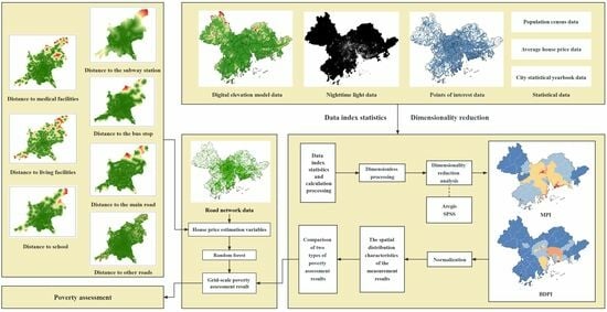
In summary, this study aims to apply multisource spatial big data to relative poverty assessment. A big data poverty index (BDPI) was constructed by integrating high-resolution Luojia 1-01 data, housing prices, and POIs. In addition, we also constructed the traditional MPI by selecting 17 indicators from six dimensions (human capital, natural capital, financial capital, physical capital, social capital, and environmental vulnerability) according to the vulnerability–sustainable livelihood analysis framework established by the Department for International Development (DFID). We compared the poverty assessment results of the BDPI and MPI to analyze the performance of these two methods. We took the Pearl River Delta in China, where the disparity between the rich and the poor is huge, as a case study area. The conclusions could provide support for local governments to formulate poverty-alleviation policies and implement development plans for underdeveloped areas.

2. Case Study and Data

2.1. Study Area

In this study, county-level administrative districts were regarded as the research unit. For clarity, we referred to all county-level administrative districts as “counties” in this manuscript. The study area includes 50 counties in the nine cities of the Pearl River Delta, of which Dongguan and Zhongshan were special cities with no counties (Figure 1). Located on the southern coast of China, the Pearl River Delta is one of the most populated areas in the Asia-Pacific region [78]. As an economically developed area, the Pearl River Delta generates 85% of Guangdong Province’s GDP and accounts for 70% of this province’s population. However, some counties in the Pearl River Delta have witnessed different degrees of relative poverty. Since it is extremely important to accurately identify relative poverty within developed regions, taking the Pearl River Delta as a case study is of universal significance [79,80,81].

2.2. Data

This study adopted data that are easy to obtain and have reasonable timeliness, including: (1) high-resolution LuoJia 1-01 nighttime light data (with a spatial resolution of 130 m) in 2018 from Wuhan University (http://www.hbeos.org.cn/, accessed on 6 May 2023) [82,83,84]. This high-quality dataset has been pre-processed by constructing the geometric processing model of the whole link network for image-to-ground target positioning, and has been geo-referenced based on the ground control points participating in the processing of regional network adjustment. Therefore, the original spatial positioning errors have been adequately corrected. Lastly, the background noise for LuoJia 1-01 nighttime light data was removed by using the same period of NPP/VIIRS image as the mask data; (2) POI data in 2018 from AutoNavi Map (https://www.amap.com/, accessed on 6 May 2023), including corporates, scenic spots, scientific, educational and cultural services, transportation facilities, living facilities, and sports and leisure services. The attributes of the POIs include the specific geographic location information and detailed information on service facilities; (3) housing price data in 2021 and 2022 from Anjuke (https://www.anjuke.com/, accessed on 6 May 2023) and Loupan (https://www.loupan.com/, accessed on 6 May 2023), two of the most influential real estate platforms in China. All the housing price data were captured through the web crawler, and each data record includes name, area, price, address, and coordinate. A total of 64,750 valid records were obtained; (4) data on social, economic, population and other basic indicators from the 2019 County-level Statistical Yearbook and the Seventh Population Census in China, including population aged 0–14 years and over 65 years old, rural population, ethnic minority population, proportion of population with primary education, proportion of population with secondary education, proportion of population with college or higher education, illiterate population over 15 years old, average years of education completed, number of professional technicians, number of people engaged in agriculture, forestry, animal husbandry and fishery, number of tertiary sectors, income in local government budget, and proportion of jobholders; (5) digital elevation model (DEM) (with a spatial resolution of 30 m) and precipitation data (with a spatial resolution of 1 km) in 2018 from the China Earth System Science Data Center (http://www.geodata.cn/, accessed on 6 May 2023); and (6) road network data in 2018 from OpenStreetMap (https://download.geofabrik.de/, accessed on 6 May 2023), including main roads and other roads.
It should be noted that there is only one high-quality pre-processed dataset of LuoJia 1-01 nighttime light remote sensing image, from the year 2018. To reduce the negative influence caused by the inconsistent data year, we collected data from the same year as much as possible. However, the housing price platforms only provide the data of the latest year; thus, we cannot obtain the housing price data of the study area in 2018. At the same time, the most recent population census data of China come from the seventh population census. Therefore, we have to adopt the house price data of 2021–2022 as well as the census data of 2019.

2.2.1. LuoJia 1-01

The radiance of LuoJia 1-01 nighttime light data was converted using the following formula given on the official website [85,86,87,88]:
L = D N 3 2 · 10 5
where L is the corrected radiance ( W / ( m 2 · s r · μ m ) ), and DN is the original digital number value of the data. The mean, maximum, standard deviation, sum, and Moran’s I Index of the converted nighttime light data for each county were regarded as the nighttime light-related indicators (Table 1).

2.2.2. POI

POI can effectively reflect socio-economic activities and urban vitality. The POI data were preprocessed to eliminate incomplete and inconsistent data. Then, we calculated the POI densities of various categories for each county.

2.2.3. Housing Price

Housing prices can comprehensively reflect the built environment, such as housing conditions, public facility configurations, traffic conditions, as well as the economic conditions of residents [89,90]. While online housing price data are available at the community level, traditional statistical data are usually available at the county level. In order to compare the performance of the MPI and BDPI, it is necessary to rescale the housing price data to the county level. Therefore, we collected housing price data and then calculated the average housing price in each county.

3. Method

As shown in Figure 2, this study includes five major steps: (1) dimensionless processing of all data; (2) reducing the dimensionality of 11 indicators related to nighttime light data, housing prices, and POIs by principal component analysis (PCA) to obtain the BDPI scores; (3) reducing the dimensionality of 17 indicators related to socioeconomic statistics by factor analysis to obtain the MPI scores; (4) comparing the spatial characteristics of these two poverty assessment results; (5) using random forest to estimate grid-scale housing price data according to road network and POI; (6) constructing grid-scale BDPI by combining grid-scale house price data, POI, and nighttime light; and (7) using the BDPI to measure grid-scale poverty conditions in the study area.

3.1. Big Data Poverty Index (BDPI)

This study integrated three types of indicators (nighttime light, housing price, POI) to construct the BDPI. First, the dimensionality of the original data was reduced by using PCA to eliminate duplicate information. Second, the dimensionally reduced data were assessed by using Kaiser–Meyer–Olkin (KMO) and Bartlett’s sphericity tests. A KMO score greater than 0.6 indicates a good performance of PCA (Table 2). Finally, the weight of each principal component was assigned based on the ratio of the variance contribution rate to the cumulative contribution rate of the principal component. Note that the sum of the variance contribution rates of all principal components is 100%. The formula for calculating the BDPI is given as follows:
B D P I i = k = 1 n α k × α i k
where α i k is the score of indicator k for the i-th county; and α k is the variance contribution rate of indicator k. A lower value of BDPI suggests a higher degree of poverty.
PCA was performed on multisource spatial data to generate the BDPI. The indicators with a factor loading greater than 0.6 were extracted as the main contribution indicators of the principal component. The results show that the first three principal components should be preserved, as they can explain approximately 79.96% of the original information (Table 3).

3.2. Multidimensional Poverty Index (MPI)

Based on the vulnerability-sustainable livelihood analysis framework and data availability, we adopted 17 indicators from 6 dimensions (human capital, natural capital, financial capital, physical capital, social capital, and environmental vulnerability). The dimensionality of the data was reduced by factor analysis, and the dimensionally reduced data were assessed by KMO and Bartlett’s tests. A KMO value greater than 0.6 indicates a good performance of the factor analysis (Table 4).
The weight of each principal component was assigned based on the ratio of the variance contribution rate to the cumulative contribution rate of the component, and the sum of the variance contribution rates of all principal components is 100%. Finally, the MPI value of each county was calculated as follows:
F i = j W j Y i j
where F i is the MPI value of the i-th county, reflecting its poverty degree; W j is the weight of the j-th common factor, which can be represented by the variance contribution rate of each common factor; and Y i j is the single-item score of the j-th common factor in the i-th county, which can be calculated from the factor score coefficient matrix and the observed value of the variable. A lower value of MPI indicates a higher degree of poverty.
Factor analysis was performed on traditional statistical data to generate MPI (Table 5). The indicators with a factor loading greater than 0.9 were extracted as the main contribution indicators of each principal component. The maximum variance method was used to obtain the rotated component matrix. The cumulative explained variance after rotation reaches 89.51%, which indicates that the information of the original data can be well preserved.

3.3. Housing Price Estimation Based on Machine Learning

Since the valid housing price data did not completely cover the study area, we need to estimate the missing data based on advanced machine learning methods [91,92]. Random forest (RF) is one of the most effective and efficient machine learning methods and has been commonly used in various research fields [93,94]. Compared with other machine learning methods, RF can effectively handle high-dimensional data and missing values [95,96]. RF regression is an algorithm based on ensemble learning that completes the regression task by building multiple decision trees and integrating their prediction results.
In RF, each decision tree is trained independently using randomly selected subsamples, which effectively reduces the risk of overfitting. For each node of the decision tree, only part of the features is considered when selecting the best partition features to improve the robustness of the model. RF offers the final regression result by averaging the prediction results of multiple decision trees. In this study, the housing price estimation model was constructed based on RF by taking points of interest, road networks as independent variables and housing price data as dependent variable, according to previous findings [74,76,77].
Specifically, the distance to subway stations, distance to bus stops, distance to main roads, distance to ordinary roads, distance to medical facilities, distance to living facilities, and distance to school were used as independent variables, and the existing house price data were used as dependent variable. Then, the model trained by the RF was further used to estimate the unknown housing price data at the grid scale. Finally, the housing price data covering all the grids of the study area were obtained, and thus the grid-scale BDPI can be further constructed.

4. Results

4.1. BDPI Results

Figure 3 presents the results of the first, second, and third principal components and the associated BDPI. These three principal components can reveal the poverty status from different dimensions. Although the main components from the PCA may only have statistical meaning, researchers can interpret the substantive meaning of every principal component based on specialized knowledge [97]. Specifically, since the first component includes five high loading factors: mean, standard deviation, scenic spots, transportation facilities, and living and leisure services, it primarily represents the relative poverty caused by the lack of social capital. In addition, the second component exhibits high loadings on sum, which primarily indicates the relative poverty caused by the lack of economic capital. Similarly, the third component primarily reflects the relative poverty caused by the living environment.
Social capital (Figure 3a) can reflect the basic resources (e.g., transportation, education, and medical conditions) within the study area and is a key indicator of poverty status. We found that YueXiu County of GuangZhou City and FuTian County of ShenZhen City had higher social capital scores and belonged to highly urbanized areas. The counties with moderate to high social capital scores were clustered in ShenZhen City and the junction of GuangZhou and FoShan Cities. By comparison, the counties located on the fringe of the Pearl River Delta generally suffer a shortage of social capital, and most of them are in ZhaoQing, JiangMen and HuiZhou Cities.
Economic capital can reflect the degree of economic development within the study area. Figure 3b indicates that the central and eastern regions of the Pearl River Delta had higher economic capital scores, forming agglomeration centers with high economic potential. Most of the counties outside agglomeration centers had lower economic capital scores and relatively low degrees of economic development.
For the dimension of the living environment (Figure 3c), most counties had moderate to high scores, which suggests that the overall living environment in the Pearl River Delta is desirable. However, there still exist some counties with a relatively poor living environment, such as HuiCheng County of HuiZhou City and DeQing County of ZhaoQing City.
Overall, the BDPI score generally gradually decreases from the center to the fringe of the study area, exhibiting an obvious spatial agglomeration pattern. The regions in the western Pearl River Delta were relatively poor since the counties with higher degrees of poverty were distributed mainly in ZhaoQing, JiangMen, and HuiZhou Cities. Nevertheless, rapidly growing cities also contain some impoverished counties, such as the CongHua and ZengCheng Counties of GuangZhou City.

4.2. MPI Results

In general, the MPI score in the Pearl River Delta also gradually decreases from the center to the fringe, and the further away from the center, the higher the poverty level (Figure 4). Relatively impoverished counties were mainly distributed in ZhaoQing, JiangMen, and HuiZhou Cities. By comparison, most well-developed counties were distributed in GuangZhou, ShenZhen, and ZhuHai Cities, all of which belong to the pilot zones of the Pearl River Delta.

4.3. Comparison of Two Poverty Assessment Results

The results of the MPI and BDPI were further compared to evaluate the rationality of the BDPI. Due to differences in the principles and calculation processes of these two methods, analyzing the ranking of the index scores (i.e., ranking according to the index score, and a lower ranking means a more severe poverty status) is more in line with the definition of relative poverty. Therefore, we quantified the consistency of these two results using the Wilcoxon signed-rank test and presented the visualization of the z-score in Figure 5. The significance level of the test is 0.898 (greater than 0.05), which indicates that there is no significant difference in the score ranking of the two poverty assessment results. According to Figure 5, we also found that these two results show similar overall trends. In summary, the above validation has indicated a strong agreement between the poverty assessment results from the BDPI and MPI.
In addition, the top 20% and top 30% impoverished counties in these two results share coincidence degrees of 70% and 87%, respectively, which also demonstrates that the impoverished counties identified by the two methods are similar (Table 6). Nevertheless, we noticed that the impoverished counties identified by the MPI are concentrated in the fringe areas of the Pearl River Delta, while the BDPI can identify underdeveloped counties in some cities with rapid economic development, such as Guangzhou and Foshan. The difference between these two poverty assessment results suggests that the MPI can effectively reveal poverty status in old urban areas with convenient infrastructure but lagging behind, whereas the BDPI is suitable for emerging-development areas that are rapidly developing but still lagging behind.
The proposed BDPI and traditional MPI have different applicabilities for identifying different types of impoverished counties. To reveal the differences between the two poverty assessment results, the MPI ranking of every county was subtracted from its BDPI ranking. The BDPI poverty degree of a county is more severe than its MPI poverty degree if the ranking difference of the county is positive. In contrast, the MPI poverty degree of the county is more severe than its BDPI poverty degree if the ranking difference of this county is negative. The result in Figure 6 shows that the counties with positive ranking differences were mainly located in FoShan, ZhongShan, DongGuan, and HuiZhou Cities, whereas the counties with negative ranking differences were generally located in ZhuHai, JiangMen, GuangZhou, and ShenZhen Cities.
Among the counties with positive ranking differences, DingHu County, DongGuan City, and ZhongShan City had relatively larger differences. After the implementation of reform and opening-up policies, these areas rapidly promoted industries and handicrafts, and the supporting facilities gradually improved. They have considerable economic capital and can easily attract a large number of migrant workers. However, these areas contain a large number of urban villages with poor living spaces and low densities of basic living facilities. Therefore, the BDPI poverty degrees of these areas were more severe than the corresponding MPI poverty degrees.
Among the counties with negative ranking differences, JinWan County, GaoMing County, and YanTian County had relatively larger differences. Most of these areas were emerging-development zones with relatively complete basic living facilities, desirable living environments, and convenient transportation systems. However, they were still economically underdeveloped compared with the developed urban districts. Therefore, the MPI poverty degrees of these counties were more severe than the corresponding BDPI poverty degrees.

4.4. Grid-Scale BDPI-Based Poverty Assessment

The above comparisons have demonstrated that the proposed BDPI is feasible and effective for poverty assessment. Therefore, this study further estimated the poverty conditions at the grid scale by taking Guangzhou and Foshan as examples. These regions were divided by a grid of 500 m × 500 m. All the independent variables and the resultant grid-scale housing price data are shown in Figure 7 and Figure 8, respectively. The training and testing accuracies of the RF model reached 0.9590 and 0.9035, respectively. This phenomenon has indicated that the RF model can effectively estimate missing housing price data at the grid scale.
Finally, the grid-scale BDPI-based poverty assessment result is displayed in Figure 9. This result was classified into five levels, and a lower level indicates a more impoverished region. It is found that the center parts are well developed. With the increase in distance from the urban center, an increasing number of counties are lagging behind to varying degrees, especially CongHua, ZengCheng, SanShui, and GaoMing Counties. For example, the southern part of the boundaries between BaiYun, LiWan, YueXiu, and TianHe Counties are in a better development condition with higher BDPI levels. By comparison, most of the eastern part of BaiYun County and NanHai and ShunDe Counties are relatively lagging behind. We also noticed that level 1 regions also exist around the regions with higher BDPI levels, such as the central and eastern parts of ShunDe County. In summary, the application of the BDPI can effectively identify relative poverty at a finer scale.

5. Discussion and Conclusions

5.1. Advantages and Disadvantages of the BDPI

The above analysis shows that compared with the MPI, the BDPI proposed by this study has three major advantages. First, the BDPI was constructed by integrating multi-source spatial big data, including high-resolution Luojia 1-01 nighttime light, housing price, and POI data. Our experiments have suggested that the proposed BDPI can identify areas that are relatively lagging behind in emerging-development cities. Second, the BDPI can reduce the cost of poverty assessment and enhance the timeliness of results due to the use of easily accessible, low-cost, and rapidly updated data. Third, the BDPI can effectively reflect social, economic, living environment, and other conditions. Therefore, it provides a new approach to poverty assessment for developing countries lacking accurate socioeconomic statistics.
It should also be noted that the people in some less developed counties are more inclined to complete housing transactions offline, and these data cannot be acquired online. Fortunately, the difference between online and offline data is not significant in many regions. In addition, as mentioned above, previous studies have demonstrated that advanced machine learning techniques can be used to estimate fine-scale housing prices based on proxy variables in regions where offline data are not available. Although there are uncertainties and limitations in data preparation, BDPI still has distinct advantages in fine-scale poverty assessment. Compared with MPI, which relies on dated indicators and periodic data collection, BDPI can capture changes in poverty status instantly and provide more timely support for policy making. In addition, the use of spatial data can reflect regional differences at a grid scale.
Notwithstanding these advantages, the BDPI still has the following disadvantages. First, online housing price data may not be available in some underdeveloped areas. In that case, advanced machine learning techniques and offline data, such as local government statistics and survey data, should be used to supplement the BDPI’s data sources. Second, the indicators used to construct the BDPI also have some limitations. Poverty is a multidimensional phenomenon involving not only social, economic, and natural aspects but also humanities, policies, and other factors. Therefore, although the BDPI can be used as an indirect indicator, the associated assessment results may overestimate or underestimate the actual poverty status, and the BDPI needs to be further enhanced. Third, it is difficult for the BDPI to assess the poverty status from a long time ago due to the unavailability of historical data. The inconsistency of data years may affect the poverty assessment results to some degree. In future research, we will adopt long-term time-series data for poverty assessment to further test the applicability of the BDPI. Fourth, we will consider more spatial big data and higher-resolution nighttime light data, compare the poverty assessment results of the Pearl River Delta with other regions, and analyze the differences in poverty issues in those regions.

5.2. Policy Recommendations

In this research, the internal development of a city is unbalanced if this city contains both counties with positive ranking differences and counties with negative ranking differences, such as DingHu County and DuanZhou County in ZhaoQing City. DingHu County has an average living environment and a relatively remote location, but as a new developing zone of ZhaoQing City, this county has desirable social and economic resources. As the central urban area of ZhaoQing City, DuanZhou County has a satisfactory living environment and relatively complete supporting facilities. However, there is basically no more space for urban expansion since the amount of land available for development is decreasing gradually. Therefore, the urban development costs are relatively higher in DuanZhou County.
Overall, the poverty assessment results obtained in this study can offer the following policy recommendations for poverty alleviation. The huge disparity between the rich and the poor in the Pearl River Delta shows that poverty-alleviation operations require not only raising social income but also reducing inequality in regional development. For areas with a shortage of social resources, it is necessary to improve the diversity of their resources, for example, enhancing infrastructures such as those for medical care, public transportation, and education, to improve urban vitality. For the fringe areas of the Pearl River Delta, which are greatly affected by natural conditions, the development strategy should be carefully designed according to local characteristics. In relatively underdeveloped areas of rapidly developing cities, the government needs to offer more support, carry out detailed strategic planning, and allocate more socioeconomic resources to areas with unbalanced development to reduce the disparity between the rich and the poor. In addition, the government should further upgrade the poverty assessment method in the context of big data and improve the accuracies and pertinence of the assessment results. Taking the Pearl River Delta region as an example, this study has demonstrated that the proposed BDPI could provide technical support for poverty assessment in many other regions.

5.3. Main Conclusions

The significance and novelty of this research are twofold. Firstly, high-resolution nighttime light and spatial big data have been integrated to construct the novel big data poverty index (BDPI) for relative poverty assessment. Secondly, a poverty assessment has been conducted in the regions with relative poverty at a grid scale after the validation of the BDPI. Both the traditional MPI and BDPI were used to assess the poverty status of the Pearl River Delta, where there is a considerable disparity between the rich and the poor. We analyzed the differences in the poverty assessment results obtained by the two methods. These two methods generated similar assessment results, which verify the effectiveness of the BDPI. Overall, the results of the two poverty assessment methods show that the poverty index gradually decreases from the center to the fringe of the study area. The counties in the western Pearl River Delta were relatively impoverished, and even fast-growing cities also contained some impoverished counties.
The statistical-based MPI is more suitable for old urban areas with convenient but obsolete infrastructures, while the BDPI is more suitable for emerging-development areas that are rapidly developing but still lagging behind. Therefore, combining these two types of indices for poverty assessment can yield optimal results if the data are well-prepared. The BDPI can also successfully replace the traditional MPI if the statistical data are not updated in time. The BDPI proposed by this study can effectively assess regional poverty status and provide a new method of poverty assessment for developing countries lacking accurate socioeconomic statistics. The results of this study could help local governments to fully understand the multidimensional characteristics of poverty and could provide decision support for formulating targeted poverty-alleviation policies.

Author Contributions

Conceptualization, J.L. (Jinyao Lin); methodology, M.L.; validation, M.L.; formal analysis, Z.J. and K.C.; investigation, Z.J. and K.C.; data curation, J.L. (Jingxi Liu); writing—original draft preparation, M.L.; visualization, M.L. and J.L. (Jingxi Liu); supervision, J.L. (Jinyao Lin); project administration, J.L. (Jinyao Lin); funding acquisition, J.L. (Jinyao Lin). All authors have read and agreed to the published version of the manuscript.

Funding

This research was funded by the Guangdong Philosophy and Social Science Foundation (Grant No. GD23XSH11), the Guangdong Basic and Applied Basic Research Foundation (Grant No. 2023A1515030300), the National Natural Science Foundation of China (Grant No. 41801307), and the Guangzhou Municipal Science and Technology Project (Grant No. 202201010289).

Data Availability Statement

The data presented in this study are available on request from the corresponding author.

Conflicts of Interest

The authors declare no conflict of interest.

References

  1. Andries, A.; Morse, S.; Murphy, R.J.; Sadhukhan, J.; Martinez-Hernandez, E.; Amezcua-Allieri, M.A.; Aburto, J. Potential of Using Night-Time Light to Proxy Social Indicators for Sustainable Development. Remote Sens. 2023, 15, 1209. [Google Scholar] [CrossRef]
  2. Asher, S.; Lunt, T.; Matsuura, R.; Novosad, P. Development Research at High Geographic Resolution: An Analysis of Night-Lights, Firms, and Poverty in India Using the SHRUG Open Data Platform. World Bank Econ. Rev. 2021, 35, 845–871. [Google Scholar] [CrossRef]
  3. Cecchini, S.; Savio, G.; Tromben, V. Mapping poverty rates in Chile with night lights and fractional multinomial models. Reg. Sci. Policy Pract. 2022, 14, 850–876. [Google Scholar] [CrossRef]
  4. Hall, O.; Dompae, F.; Wahab, I.; Dzanku, F.M. A review of machine learning and satellite imagery for poverty prediction: Implications for development research and applications. J. Int. Dev. 2023, 1–16. [Google Scholar] [CrossRef]
  5. Hutasavi, S.; Chen, D. Exploring the industrial growth and poverty alleviation through space-time data mining from night-time light images: A case study in Eastern Economic Corridor (EEC), Thailand. Int. J. Remote Sens. 2022, 1–23. [Google Scholar] [CrossRef]
  6. Wang, Y.; Wang, M.; Huang, B.; Li, S.; Lin, Y. Evaluation and Analysis of Poverty-Stricken Counties under the Framework of the UN Sustainable Development Goals: A Case Study of Hunan Province, China. Remote Sens. 2021, 13, 4778. [Google Scholar] [CrossRef]
  7. Hu, S.; Ge, Y.; Liu, M.; Ren, Z.; Zhang, X. Village-level poverty identification using machine learning, high-resolution images, and geospatial data. Int. J. Appl. Earth Obs. Geoinf. 2022, 107, 102694. [Google Scholar] [CrossRef]
  8. Liu, Y.; Liu, J.; Zhou, Y. Spatio-temporal patterns of rural poverty in China and targeted poverty alleviation strategies. J. Rural Stud. 2017, 52, 66–75. [Google Scholar] [CrossRef]
  9. Wang, W.; Cheng, H.; Zhang, L. Poverty assessment using DMSP/OLS night-time light satellite imagery at a provincial scale in China. Adv. Space Res. 2012, 49, 1253–1264. [Google Scholar] [CrossRef]
  10. Luo, E.; Kuffer, M.; Wang, J. Urban poverty maps—From characterising deprivation using geo-spatial data to capturing deprivation from space. Sustain. Cities Soc. 2022, 84, 104033. [Google Scholar] [CrossRef]
  11. Määttä, I.; Ferreira, T.; Leßmann, C. Nighttime lights and wealth in very small areas. Rev. Reg. Res. 2022, 42, 161–190. [Google Scholar] [CrossRef]
  12. Xu, L.; Deng, X.; Jiang, Q.O.; Ma, F. Identification and alleviation pathways of multidimensional poverty and relative poverty in counties of China. J. Geogr. Sci. 2021, 31, 1715–1736. [Google Scholar] [CrossRef]
  13. Tselios, V.; Stathakis, D.; Faraslis, I. Concentration of populations and economic activities, growth, and convergence in Europe using satellite-observed lighting. Geocarto Int. 2020, 35, 1527–1552. [Google Scholar] [CrossRef]
  14. Tarozzi, A.; Deaton, A. Using Census and Survey Data to Estimate Poverty and Inequality for Small Areas. Rev. Econ. Stat. 2009, 91, 773–792. [Google Scholar] [CrossRef]
  15. Gu, Z.; Zhao, X.; Huang, P.; Pu, J.; Shi, X.; Li, Y. Identification of Multi-Dimensional Relative Poverty and Governance Path at the Village Scale in an Alpine-Gorge Region: A Case Study in Nujiang, China. Int. J. Environ. Res. Public Health 2023, 20, 1286. [Google Scholar] [CrossRef] [PubMed]
  16. Li, G.; Cai, Z.; Liu, X.; Liu, J.; Su, S. A comparison of machine learning approaches for identifying high-poverty counties: Robust features of DMSP/OLS night-time light imagery. Int. J. Remote Sens. 2019, 40, 5716–5736. [Google Scholar] [CrossRef]
  17. Mahabir, R.; Agouris, P.; Stefanidis, A.; Croitoru, A.; Crooks, A.T. Detecting and mapping slums using open data: A case study in Kenya. Int. J. Digit. Earth 2020, 13, 683–707. [Google Scholar] [CrossRef]
  18. Small, C.; Sousa, D.; Yetman, G.; Elvidge, C.; MacManus, K. Decades of urban growth and development on the Asian megadeltas. Glob. Planet. Chang. 2018, 165, 62–89. [Google Scholar] [CrossRef]
  19. Chen, R.; Zhang, F.; Chan, N.W.; Wang, Y. Multidimensional poverty measurement and spatial–temporal pattern analysis at county level in the arid area of Xinjiang, China. Environ. Dev. Sustain. 2022, 1–20. [Google Scholar] [CrossRef]
  20. Han, Y.; Liu, L.; Sui, Q.; Zhou, J. Big Data Spatio-Temporal Correlation Analysis and LRIM Model Based Targeted Poverty Alleviation through Education. ISPRS Int. J. Geo-Inf. 2021, 10, 837. [Google Scholar] [CrossRef]
  21. Ke, N.; Lu, X.; Kuang, B.; Zhang, X. Regional disparities and evolution trend of city-level carbon emission intensity in China. Sustain. Cities Soc. 2023, 88, 104288. [Google Scholar] [CrossRef]
  22. Ma, L.; Che, X.; Zhang, J.; Fang, F.; Chen, M. Rural Poverty Identification and Comprehensive Poverty Assessment Based on Quality-of-Life: The Case of Gansu Province (China). Sustainability 2019, 11, 4547. [Google Scholar] [CrossRef]
  23. Su, S.; Gong, Y.; Tan, B.; Pi, J.; Weng, M.; Cai, Z. Area Social Deprivation and Public Health: Analyzing the Spatial Non-stationary Associations Using Geographically Weighed Regression. Soc. Indic. Res. 2017, 133, 819–832. [Google Scholar] [CrossRef]
  24. Sun, J.; Di, L.; Sun, Z.; Wang, J.; Wu, Y. Estimation of GDP Using Deep Learning With NPP-VIIRS Imagery and Land Cover Data at the County Level in CONUS. IEEE J. Sel. Top. Appl. Earth Obs. Remote Sens. 2020, 13, 1400–1415. [Google Scholar] [CrossRef]
  25. Li, G.; Cai, Z.; Liu, J.; Liu, X.; Su, S.; Huang, X.; Li, B. Multidimensional Poverty in Rural China: Indicators, Spatiotemporal Patterns and Applications. Soc. Indic. Res. 2019, 144, 1099–1134. [Google Scholar] [CrossRef]
  26. Jean, N.; Burke, M.; Xie, M.; Davis, W.M.; Lobell, D.B.; Ermon, S. Combining satellite imagery and machine learning to predict poverty. Science 2016, 353, 790–794. [Google Scholar] [CrossRef]
  27. Elvidge, C.D.; Sutton, P.C.; Ghosh, T.; Tuttle, B.T.; Baugh, K.E.; Bhaduri, B.; Bright, E. A global poverty map derived from satellite data. Comput. Geosci. 2009, 35, 1652–1660. [Google Scholar] [CrossRef]
  28. Sutton, P.C.; Elvidge, C.D.; Ghosh, T. Estimation of Gross Domestic Product at Sub-National Scales using Nighttime Satellite Imagery. Int. J. Ecol. Econ. Stat. 2007, 8, 5–21. [Google Scholar]
  29. Levin, N.; Zhang, Q. A global analysis of factors controlling VIIRS nighttime light levels from densely populated areas. Remote Sens. Environ. 2017, 190, 366–382. [Google Scholar] [CrossRef]
  30. Pandey, B.; Joshi, P.K.; Seto, K.C. Monitoring urbanization dynamics in India using DMSP/OLS night time lights and SPOT-VGT data. Int. J. Appl. Earth Obs. Geoinf. 2013, 23, 49–61. [Google Scholar] [CrossRef]
  31. Zhuo, L.; Shi, Q.; Tao, H.; Zheng, J.; Li, Q. An improved temporal mixture analysis unmixing method for estimating impervious surface area based on MODIS and DMSP-OLS data. ISPRS J. Photogramm. Remote Sens. 2018, 142, 64–77. [Google Scholar] [CrossRef]
  32. Zhang, Q.; Seto, K.C. Mapping urbanization dynamics at regional and global scales using multi-temporal DMSP/OLS nighttime light data. Remote Sens. Environ. 2011, 115, 2320–2329. [Google Scholar] [CrossRef]
  33. Bennett, M.M.; Smith, L.C. Advances in using multitemporal night-time lights satellite imagery to detect, estimate, and monitor socioeconomic dynamics. Remote Sens. Environ. 2017, 192, 176–197. [Google Scholar] [CrossRef]
  34. Cao, X.; Wang, J.; Chen, J.; Shi, F. Spatialization of electricity consumption of China using saturation-corrected DMSP-OLS data. Int. J. Appl. Earth Obs. Geoinf. 2014, 28, 193–200. [Google Scholar] [CrossRef]
  35. Elvidge, C.D.; Baugh, K.; Zhizhin, M.; Hsu, F.C.; Ghosh, T. VIIRS night-time lights. Int. J. Remote Sens. 2017, 38, 5860–5879. [Google Scholar] [CrossRef]
  36. Ghosh, T.; Anderson, S.J.; Elvidge, C.D.; Sutton, P.C. Using Nighttime Satellite Imagery as a Proxy Measure of Human Well-Being. Sustainability 2013, 5, 4988–5019. [Google Scholar] [CrossRef]
  37. He, C.; Ma, Q.; Liu, Z.; Zhang, Q. Modeling the spatiotemporal dynamics of electric power consumption in Mainland China using saturation-corrected DMSP/OLS nighttime stable light data. Int. J. Digit. Earth 2014, 7, 993–1014. [Google Scholar] [CrossRef]
  38. Ma, T.; Zhou, C.; Pei, T.; Haynie, S.; Fan, J. Responses of Suomi-NPP VIIRS-derived nighttime lights to socioeconomic activity in China’s cities. Remote Sens. Lett. 2014, 5, 165–174. [Google Scholar] [CrossRef]
  39. Mellander, C.; Lobo, J.; Stolarick, K.; Matheson, Z. Night-Time Light Data: A Good Proxy Measure for Economic Activity? PLoS ONE 2015, 10, e0139779. [Google Scholar] [CrossRef]
  40. Pan, J.; Li, J. Spatiotemporal Dynamics of Electricity Consumption in China. Appl. Spat. Anal. Policy 2019, 12, 395–422. [Google Scholar] [CrossRef]
  41. Yong, Z.; Li, K.; Xiong, J.; Cheng, W.; Wang, Z.; Sun, H.; Ye, C. Integrating DMSP-OLS and NPP-VIIRS Nighttime Light Data to Evaluate Poverty in Southwestern China. Remote Sens. 2022, 14, 600. [Google Scholar] [CrossRef]
  42. Liu, H.; Wang, J.; Liu, H.; Chen, Y.; Liu, X.; Guo, Y.; Huang, H. Identification of Relative Poverty Based on 2012-2020 NPP/VIIRS Night Light Data: In the Area Surrounding Beijing and Tianjin in China. Sustainability 2022, 14, 5559. [Google Scholar] [CrossRef]
  43. Yu, B.; Shi, K.; Hu, Y.; Huang, C.; Chen, Z.; Wu, J. Poverty Evaluation Using NPP-VIIRS Nighttime Light Composite Data at the County Level in China. IEEE J. Sel. Top. Appl. Earth Obs. Remote Sens. 2015, 8, 1217–1229. [Google Scholar] [CrossRef]
  44. Pan, J.; Hu, Y. Spatial Identification of Multi-dimensional Poverty in Rural China: A Perspective of Nighttime-Light Remote Sensing Data. J. Indian Soc. Remote Sens. 2018, 46, 1093–1111. [Google Scholar] [CrossRef]
  45. Coscieme, L.; Sutton, P.C.; Anderson, S.; Liu, Q.; Elvidge, C.D. Dark Times: Nighttime satellite imagery as a detector of regional disparity and the geography of conflict. GISci. Remote Sens. 2017, 54, 118–139. [Google Scholar] [CrossRef]
  46. Georganos, S.; Abascal, A.; Kuffer, M.; Wang, J.; Owusu, M.; Wolff, E.; Vanhuysse, S. Is It All the Same? Mapping and Characterizing Deprived Urban Areas Using WorldView-3 Superspectral Imagery. A Case Study in Nairobi, Kenya. Remote Sens. 2021, 13, 4986. [Google Scholar] [CrossRef]
  47. Gibson, J.; Olivia, S.; Boe-Gibson, G.; Li, C. Which night lights data should we use in economics, and where? J. Dev. Econ. 2021, 149, 102602. [Google Scholar] [CrossRef]
  48. Proville, J.; Zavala-Araiza, D.; Wagner, G. Night-time lights: A global, long term look at links to socio-economic trends. PLoS ONE 2017, 12, e0174610. [Google Scholar] [CrossRef]
  49. Putri, S.R.; Wijayanto, A.W.; Sakti, A.D. Developing Relative Spatial Poverty Index Using Integrated Remote Sensing and Geospatial Big Data Approach: A Case Study of East Java, Indonesia. ISPRS Int. J. Geo-Inf. 2022, 11, 275. [Google Scholar] [CrossRef]
  50. Puttanapong, N.; Martinez, A.; Bulan, J.A.N.; Addawe, M.; Durante, R.L.; Martillan, M. Predicting Poverty Using Geospatial Data in Thailand. ISPRS Int. J. Geo-Inf. 2022, 11, 293. [Google Scholar] [CrossRef]
  51. Chen, Q.; Ye, T.; Zhao, N.; Ding, M.; Ouyang, Z.; Jia, P.; Yue, W.; Yang, X. Mapping China’s regional economic activity by integrating points-of-interest and remote sensing data with random forest. Environ. Plan. B Urban Anal. City Sci. 2021, 48, 1876–1894. [Google Scholar] [CrossRef]
  52. Du, X.; Shen, L.; Wong, S.W.; Meng, C.; Yang, Z. Night-time light data based decoupling relationship analysis between economic growth and carbon emission in 289 Chinese cities. Sustain. Cities Soc. 2021, 73, 103119. [Google Scholar] [CrossRef]
  53. Roy Chowdhury, P.K.; Weaver, J.E.; Weber, E.M.; Lunga, D.; LeDoux, S.T.M.; Rose, A.N.; Bhaduri, B.L. Electricity consumption patterns within cities: Application of a data-driven settlement characterization method. Int. J. Digit. Earth 2020, 13, 119–135. [Google Scholar] [CrossRef]
  54. Pokhriyal, N.; Jacques, D.C. Combining disparate data sources for improved poverty prediction and mapping. Proc. Natl. Acad. Sci. USA 2017, 114, E9783–E9792. [Google Scholar] [CrossRef] [PubMed]
  55. Guo, W.; Zhang, J.; Zhao, X.; Li, Y.; Liu, J.; Sun, W.; Fan, D. Combining Luojia1-01 Nighttime Light and Points-of-Interest Data for Fine Mapping of Population Spatialization Based on the Zonal Classification Method. IEEE J. Sel. Top. Appl. Earth Obs. Remote Sens. 2023, 16, 1589–1600. [Google Scholar] [CrossRef]
  56. Davis, M.A.; Ortalo-Magné, F. Household expenditures, wages, rents. Rev. Econ. Dyn. 2011, 14, 248–261. [Google Scholar] [CrossRef]
  57. Partridge, M.D.; Rickman, D.S.; Ali, K.; Olfert, M.R. Recent spatial growth dynamics in wages and housing costs: Proximity to urban production externalities and consumer amenities. Reg. Sci. Urban Econ. 2010, 40, 440–452. [Google Scholar] [CrossRef]
  58. Ni, Y.; Li, X.; Ye, Y.; Li, Y.; Li, C.; Chu, D. An Investigation on Deep Learning Approaches to Combining Nighttime and Daytime Satellite Imagery for Poverty Prediction. IEEE Geosci. Remote Sens. Lett. 2021, 18, 1545–1549. [Google Scholar] [CrossRef]
  59. Shi, K.; Chang, Z.; Chen, Z.; Wu, J.; Yu, B. Identifying and evaluating poverty using multisource remote sensing and point of interest (POI) data: A case study of Chongqing, China. J. Clean. Prod. 2020, 255, 120245. [Google Scholar] [CrossRef]
  60. Lin, J.; Luo, S.; Huang, Y. Poverty estimation at the county level by combining LuoJia1-01 nighttime light data and points of interest. Geocarto Int. 2022, 37, 3590–3606. [Google Scholar] [CrossRef]
  61. Lin, L.; Di, L.; Zhang, C.; Guo, L.; Di, Y. Remote Sensing of Urban Poverty and Gentrification. Remote Sens. 2021, 13, 4022. [Google Scholar] [CrossRef]
  62. Ma, T. Quantitative responses of satellite-derived night-time light signals to urban depopulation during Chinese New Year. Remote Sens. Lett. 2019, 10, 139–148. [Google Scholar] [CrossRef]
  63. Shi, K.; Wu, Y.; Liu, S.; Chen, Z.; Huang, C.; Cui, Y. Mapping and evaluating global urban entities (2000–2020): A novel perspective to delineate urban entities based on consistent nighttime light data. GIScience Remote Sens. 2023, 60, 2161199. [Google Scholar] [CrossRef]
  64. Tan, Y.; Wu, P.; Zhou, G.; Li, Y.; Bai, B. Combining Residual Neural Networks and Feature Pyramid Networks to Estimate Poverty Using Multisource Remote Sensing Data. IEEE J. Sel. Top. Appl. Earth Obs. Remote Sens. 2020, 13, 553–565. [Google Scholar] [CrossRef]
  65. Wu, J.; Wang, Z.; Li, W.; Peng, J. Exploring factors affecting the relationship between light consumption and GDP based on DMSP/OLS nighttime satellite imagery. Remote Sens. Environ. 2013, 134, 111–119. [Google Scholar] [CrossRef]
  66. Xu, J.; Song, J.; Li, B.; Liu, D.; Cao, X. Combining night time lights in prediction of poverty incidence at the county level. Appl. Geogr. 2021, 135, 102552. [Google Scholar] [CrossRef]
  67. Wang, K.; Zhang, L.; Cai, M.; Liu, L.; Wu, H.; Peng, Z. Measuring Urban Poverty Spatial by Remote Sensing and Social Sensing Data: A Fine-Scale Empirical Study from Zhengzhou. Remote Sens. 2023, 15, 381. [Google Scholar] [CrossRef]
  68. Xu, Y.; Mo, Y.; Zhu, S. Poverty Mapping in the Dian-Gui-Qian Contiguous Extremely Poor Area of Southwest China Based on Multi-Source Geospatial Data. Sustainability 2021, 13, 8717. [Google Scholar] [CrossRef]
  69. Yin, J.; Qiu, Y.; Zhang, B. Identification of Poverty Areas by Remote Sensing and Machine Learning: A Case Study in Guizhou, Southwest China. ISPRS Int. J. Geo-Inf. 2021, 10, 11. [Google Scholar] [CrossRef]
  70. Zhao, X.; Yu, B.; Liu, Y.; Chen, Z.; Li, Q.; Wang, C.; Wu, J. Estimation of Poverty Using Random Forest Regression with Multi-Source Data: A Case Study in Bangladesh. Remote Sens. 2019, 11, 375. [Google Scholar] [CrossRef]
  71. Zhao, N.; Liu, Y.; Hsu, F.-C.; Samson, E.L.; Letu, H.; Liang, D.; Cao, G. Time series analysis of VIIRS-DNB nighttime lights imagery for change detection in urban areas: A case study of devastation in Puerto Rico from hurricanes Irma and Maria. Appl. Geogr. 2020, 120, 102222. [Google Scholar] [CrossRef]
  72. Kraff, N.J.; Wurm, M.; Taubenböck, H. Housing forms of poverty in Europe—A categorization based on literature research and satellite imagery. Appl. Geogr. 2022, 149, 102820. [Google Scholar] [CrossRef]
  73. Delang, C.O.; Lung, H.C. Public Housing and Poverty Concentration in Urban Neighbourhoods: The Case of Hong Kong in the 1990s. Urban Stud. 2010, 47, 1391–1413. [Google Scholar] [CrossRef]
  74. Zhang, P.; Hu, S.; Li, W.; Zhang, C.; Yang, S.; Qu, S. Modeling fine-scale residential land price distribution: An experimental study using open data and machine learning. Appl. Geogr. 2021, 129, 102442. [Google Scholar] [CrossRef]
  75. Yi, C.; Huang, Y. Housing Consumption and Housing Inequality in Chinese Cities During the First Decade of the Twenty-First Century. Hous. Stud. 2014, 29, 291–311. [Google Scholar] [CrossRef]
  76. Zhou, X.; Tong, W.; Li, D. Modeling Housing Rent in the Atlanta Metropolitan Area Using Textual Information and Deep Learning. ISPRS Int. J. Geo-Inf. 2019, 8, 349. [Google Scholar] [CrossRef]
  77. Yao, Y.; Zhang, J.; Hong, Y.; Liang, H.; He, J. Mapping fine-scale urban housing prices by fusing remotely sensed imagery and social media data. Trans. GIS 2018, 22, 561–581. [Google Scholar] [CrossRef]
  78. Lin, J.; Qiu, S.; Tan, X.; Zhuang, Y. Measuring the relationship between morphological spatial pattern of green space and urban heat island using machine learning methods. Build. Environ. 2023, 228, 109910. [Google Scholar] [CrossRef]
  79. Yuan, Y.; Wu, F. The development of the index of multiple deprivations from small-area population census in the city of Guangzhou, PRC. Habitat Int. 2014, 41, 142–149. [Google Scholar] [CrossRef]
  80. Chen, Q.; Hou, X.; Zhang, X.; Ma, C. Improved GDP spatialization approach by combining land-use data and night-time light data: A case study in China’s continental coastal area. Int. J. Remote Sens. 2016, 37, 4610–4622. [Google Scholar] [CrossRef]
  81. Lin, J.; Zhang, W.; Wen, Y.; Qiu, S. Evaluating the association between morphological characteristics of urban land and pluvial floods using machine learning methods. Sustain. Cities Soc. 2023, 104891. [Google Scholar] [CrossRef]
  82. Li, C.; Yang, W.; Tang, Q.; Tang, X.; Lei, J.; Wu, M.; Qiu, S. Detection of Multidimensional Poverty Using Luojia 1-01 Nighttime Light Imagery. J. Indian Soc. Remote Sens. 2020, 48, 963–977. [Google Scholar] [CrossRef]
  83. Li, X.; Li, X.; Li, D.; He, X.; Jendryke, M. A preliminary investigation of Luojia-1 night-time light imagery. Remote Sens. Lett. 2019, 10, 526–535. [Google Scholar] [CrossRef]
  84. Zhang, G.; Guo, X.; Li, D.; Jiang, B. Evaluating the Potential of LJ1-01 Nighttime Light Data for Modeling Socio-Economic Parameters. Sensors 2019, 19, 1465. [Google Scholar] [CrossRef] [PubMed]
  85. Li, X.; Zhao, L.; Li, D.; Xu, H. Mapping Urban Extent Using Luojia 1-01 Nighttime Light Imagery. Sensors 2018, 18, 3665. [Google Scholar] [CrossRef] [PubMed]
  86. Lu, Y.; Liang, Y.; Lu, S.; Xiao, Y.; He, X.; Lin, J. Spatialization of carbon emissions in Guangzhou City by combining Luojia1-01 nighttime light and urban functional zoning data. J. Geo-Inf. Sci. 2022, 24, 1176–1188. [Google Scholar] [CrossRef]
  87. Zhang, G.; Li, L.; Jiang, Y.; Shen, X.; Li, D. On-Orbit Relative Radiometric Calibration of the Night-Time Sensor of the LuoJia1-01 Satellite. Sensors 2018, 18, 4225. [Google Scholar] [CrossRef]
  88. Guo, W.; Li, G.; Ni, W.; Zhang, Y.; Lu, D. Exploring improvement of impervious surface estimation at national scale through integration of nighttime light and Proba-V data. GIScience Remote Sens. 2018, 55, 699–717. [Google Scholar] [CrossRef]
  89. Niu, T.; Chen, Y.; Yuan, Y. Measuring urban poverty using multi-source data and a random forest algorithm: A case study in Guangzhou. Sustain. Cities Soc. 2020, 54, 102014. [Google Scholar] [CrossRef]
  90. Meng, Y.; Xing, H.; Yuan, Y.; Wong, M.S.; Fan, K. Sensing urban poverty: From the perspective of human perception-based greenery and open-space landscapes. Comput. Environ. Urban Syst. 2020, 84, 101544. [Google Scholar] [CrossRef]
  91. Truong, Q.; Nguyen, M.; Dang, H.; Mei, B. Housing Price Prediction via Improved Machine Learning Techniques. Procedia Comput. Sci. 2020, 174, 433–442. [Google Scholar] [CrossRef]
  92. Rana, V.S.; Mondal, J.; Sharma, A.; Kashyap, I. House Price Prediction Using Optimal Regression Techniques. In Proceedings of the 2020 2nd International Conference on Advances in Computing, Communication Control and Networking (ICACCCN), Greater Noida, India, 18–19 December 2020; pp. 203–208. [Google Scholar]
  93. Stevens, F.R.; Gaughan, A.E.; Linard, C.; Tatem, A.J. Disaggregating Census Data for Population Mapping Using Random Forests with Remotely-Sensed and Ancillary Data. PLoS ONE 2015, 10, e0107042. [Google Scholar] [CrossRef] [PubMed]
  94. Zeng, J.; Zhang, R.; Tang, J.; Liang, J.; Li, J.; Zeng, Y.; Li, Y.; Zhang, Q.; Shui, W.; Wang, Q. Ecological sustainability assessment of the carbon footprint in Fujian Province, southeast China. Front. Earth Sci. 2021, 15, 12–22. [Google Scholar] [CrossRef]
  95. Breiman, L. Random Forests. Mach. Learn. 2001, 45, 5–32. [Google Scholar] [CrossRef]
  96. Li, H.; Peng, Y.; Li, M.; Zhuang, Y.; He, X.; Lin, J. Analyzing spatial patterns and influencing factors of different illegal land use types within ecological spaces: A case study of a fast-growing city. J. Clean. Prod. 2023, 138883. [Google Scholar] [CrossRef]
  97. Interpret the Key Results for Principal Components Analysis. Available online: https://support.minitab.com/en-us/minitab/21/help-and-how-to/statistical-modeling/multivariate/how-to/principal-components/interpret-the-results/key-results/ (accessed on 6 May 2023).
Figure 1. Administrative divisions of the Pearl River Delta.
Remotesensing 15 04618 g001
Figure 2. Poverty index construction and poverty assessment based on multisource spatial big data.
Remotesensing 15 04618 g002
Figure 3. Results of the (a) first, (b) second, (c) third principal components, and (d) BDPI.
Remotesensing 15 04618 g003
Figure 4. MPI-based poverty assessment result.
Remotesensing 15 04618 g004
Figure 5. Z-scores of the results from BDPI and MPI.
Remotesensing 15 04618 g005
Figure 6. Differences between the two poverty assessment results.
Remotesensing 15 04618 g006
Figure 7. Independent variables for housing price estimation.
Remotesensing 15 04618 g007
Figure 8. Grid-scale housing price data.
Remotesensing 15 04618 g008
Figure 9. Grid-scale BDPI-based poverty assessment result.
Remotesensing 15 04618 g009
Table 1. Indicators for measuring nighttime light data.
IndicatorExplanation
Average valueL/G, L means the total values of all land use grids, G means the number of grids
Average light indexL/ G 0 , G 0 means the number of land use grids in lighting parts
Standard deviation i = 1 G ( x i x ¯ ) 2 G 1 ,     x i means the value for the ith grid, x ¯ means the average score for every grid
Maximum valueMaximum value for every land use grid
Moran’s I IndexRelationship between pixel light values for each county, which represents spatial correlation
Table 2. KMO and Bartlett’s test for the BDPI.
KMO0.635
Bartlett’s testDegree of freedom55
Significance0.000
Table 3. BDPI indicators, principal factor eigenvalues, explanatory contribution, and load matrix.
CategoryIndicatorPrincipal Component
FirstSecondThird
Nighttime lightMean0.952
Maximum 0.639
Standard Deviation0.847
Sum 0.890
Moran’s I Index−0.603
POICorporates
Scenic spots0.875
Scientific, educational and cultural services0.689
Transportation facilities 0.938
Living and leisure services0.930
Housing priceAverage housing price −0.836
Eigenvalue of the principal component5.6901.8121.294
Contribution rate of the principal component (%)51.72916.47311.763
Cumulative contribution rate of the principal components (%)51.72968.20279.964
Table 4. KMO and Bartlett’s tests for the MPI.
KMO0.794
Bartlett’s testDegree of freedom136
Significance0.000
Table 5. MPI indicators, principal factor eigenvalues, explanatory contribution, and load matrix.
IndicatorPrincipal Component
FirstSecondThirdFourthFifth
Population aged 0–14 years and over 65 years old0.917
Rural population0.894
Ethnic minority population −0.595
Proportion of population with primary education−0.861
Proportion of population with secondary education −0.908
Proportion of population with college or higher education 0.800
Illiterate population over 15 years old0.829
Average years of education completed0.737
Number of professional technicians 0.764
Number of people engaged in agriculture, forestry, animal husbandry and fishery0.914
Number of tertiary sectors 0.873
Income in local government budget 0.807
Proportion of jobholders 0.587
Average elevation 0.948
Average topographic relief 0.926
Proportion of areas with slopes greater than 15° 0.901
Average precipitation 0.954
Eigenvalue of the principal component7.9052.8522.2831.1990.978
Rotated variance contribution rate of the principal component (%)33.99625.05116.4207.0756.965
Cumulative variance contribution rate of the principal component (%)33.99659.04775.46682.54189.506
Table 6. Consistency and difference between the results from BDPI and MPI.
Top N%CityNumber of Impoverished County
BDPIMPI
Top 20%Guangzhou10
Dongguan00
Zhongshan00
Foshan10
Huizhou13
Jiangmen10
Shenzhen00
Zhuhai11
ZhaoQing56
Top 30%Guangzhou11
Dongguan00
Zhongshan00
Foshan10
Huizhou13
Jiangmen43
Shenzhen00
Zhuhai21
Zhaoqing67
Disclaimer/Publisher’s Note: The statements, opinions and data contained in all publications are solely those of the individual author(s) and contributor(s) and not of MDPI and/or the editor(s). MDPI and/or the editor(s) disclaim responsibility for any injury to people or property resulting from any ideas, methods, instructions or products referred to in the content.

