Article

Novel Land Cover Change Detection Deep Learning Framework with Very Small Initial Samples Using Heterogeneous Remote Sensing Images

1
School of Economics and Management, Xi’an Shiyou University, Xi’an 710065, China
2
School of Computer Science and Engineering, Xi’an University of Technology, Xi’an 710048, China
3
Climate & Ecosystem Sciences Division, Lawrence Berkeley National Laboratory, Berkeley, CA 94720, USA
*
Author to whom correspondence should be addressed.
Remote Sens. 2023, 15(18), 4609; https://doi.org/10.3390/rs15184609
Submission received: 13 August 2023 / Revised: 9 September 2023 / Accepted: 18 September 2023 / Published: 19 September 2023

Abstract

:
Change detection with heterogeneous remote sensing images (Hete-CD) plays a significant role in practical applications, particularly in cases where homogenous remote sensing images are unavailable. However, directly comparing bitemporal heterogeneous remote sensing images (HRSIs) to measure the change magnitude is unfeasible. Numerous deep learning methods require substantial samples to train the module adequately. Moreover, the process of labeling a large number of samples for land cover change detection using HRSIs is time-consuming and labor-intensive. Consequently, deep learning networks face challenges in achieving satisfactory performance in Hete-CD due to the limited number of training samples. This study proposes a novel deep-learning framework for Hete-CD to achieve satisfactory performance even with a limited number of initial samples. We developed a multiscale network with a selected kernel-attention module. This design allows us to effectively capture different change targets characterized by diverse sizes and shapes. In addition, a simple yet effective non-parameter sample-enhanced algorithm that utilizes the Pearson correlation coefficient is proposed to explore the potential samples surrounding every initial sample. The proposed network and sample-enhanced algorithm are integrated into an iterative framework to improve change detection performance with a limited number of small samples. The experimental results were achieved based on four pairs of real HRSIs, which were acquired with Landsat-5, Radarsat-2, and Sentinel-2 satellites with optical and SAR sensors. Results indicated that the proposed framework could achieve competitive accuracy with a small number of samples compared with some state-of-the-art methods, including three traditional methods and nine state-of-the-art deep learning methods. For example, the improvement rates are approximately 3.38% and 1.99% compared with the selected traditional methods and deep learning methods, respectively.

1. Introduction

Land cover change detection (LCCD) using remote sensing images involves comparing the bitemporal images and extracting the land cover change [1,2], such as the land cover change before and after some land cover change events, such as a landslide or wildfire events. In this study, the task of land cover change detection on the earth’s surface was accomplished by comparing the images that cover the same geographical area but were acquired at different dates. LCCD using remote sensing images can capture large-scale land changes on the earth’s surface [3]. The land cover change information plays a vital role in landslide and earthquake inventory mapping [4,5,6], environmental quality assessment [7,8,9], natural resource monitoring [10,11], urban development decision-making [12,13,14], crop yield estimation [15], and other applications [16]. Therefore, LCCD with remote sensing images is attractive for practical applications [16,17,18,19].
Over the past decades, various LCCD methods have been developed. These methods can be divided into two major groups based on the type of bitemporal images used [20]: change detection with homogeneous remote sensing images (Homo-CD) and change detection with heterogeneous remote sensing images (Hete-CD). The details of each group were reviewed as follows:
Homo-CD indicates that the images used for LCCD are homogeneous data acquired with the same remote sensors, possess similar spatial-spectral resolution, and exhibit consistent reflectance signatures [16]. Accordingly, the images can be directly compared to determine the magnitude of the change and acquire land cover change information. Researchers have proposed several methods for Homo-CD. One of the most popular methods is the contextual information-based method [19], such as the sliding window-based approach [21], the mathematical model-based method [22], and the adaptive region-based approach [23,24]. Deep learning methods for Homo-CD, such as convolutional neural networks [25,26,27] and fully convolutional Siamese networks [28,29], have also been widely used. Many deep learning networks have been developed with multiscale convolution [30,31] and deep feature fusion [32,33] to cover more ground targets and utilize deep features. Moreover, change trend detection with multitemporal images has been attractive and popular in recent years [17,34,35]. Although various change detection methods have been developed and have showcased excellent performance, demonstrating their feasibility and advantages for Homo-CD, two major drawbacks persist: Deep learning neural network training requires considerable samples, and preparing a large number of training samples is labor-intensive and time-consuming.
Homogeneous images may be unavailable in numerous application scenarios due to the physical limitations of remote sensing sensors. For example, optical satellite images are typically unavailable for detecting land cover change caused by nighttime wildfires or floods [20]. Nevertheless, pre-event optical images are easily obtained with satellites. In addition, the image quality of optical satellite images is easily affected by weather [36,37]. Therefore, to address the limitations of Homo-CD in practical applications, Hete-CD is proposed and has gained popularity in recent years [38].
In contrast with Homo-CD, the images used for Hete-CD are heterogeneous remote sensing images (HRSIs). The HRSIs have an advantage in complementing the insignificance of homogeneous images, such as an optical image reflecting the appearance of ground targets by visible, near-infrared, and short-wave infrared sensors. Consequently, the illumination and atmospheric conditions significantly affect the optical image quality. Meanwhile, a synthetic aperture radar (SAR) image depicts the physical scattering of ground targets. The appearance of a target in a SAR image depends on its roughness and microwave energy wavelength. When an optical image is available prior to a night flood or landslide, a SAR image is an alternative after a disaster because it is independent of visual light and weather conditions [39]. Accordingly, immediate assessment of the damage caused by natural disasters using optical and SAR images is possible in certain urgent cases. The superiority of Hete-CD increases the corresponding demand for practical engineering.
Various methods have been promoted for Hete-CD in recent years. The most popular approach to Hete-CD focused on exploring the shared features and measuring the similarity between the shared features and bitemporal HRSIs. Wan et al. [40] explored the statistical features of multisensor images for LCCD. Lei et al. [41] extracted the adaptive local structure from HRSIs for Hete-CD. Sun et al. [42] improved the adaptive structure feature based on sparse theory for Hete-CD. Moreover, techniques such as image regression [43,44,45], graph representation theory [46,47,48,49,50], and pixel transformation [51] can be effectively used to investigate the mutual features needed to carry out change detection tasks with HRSIs. Although considerable traditional methods and their applications have demonstrated the feasibility and advantages of using HRSIs in LCCD, these algorithms are typically complex, and their optimal parameter involves trial-and-error experiments.
However, the aforementioned traditional methods aim at exploring the features that are focused on describing the pixel’s relationship [52,53]. In recent years, deep learning techniques have been promoted and widely used in the fields of computer vision [54] and change detection [55]. Particularly, deep learning techniques have been frequently used to analyze deep features from HRSIs and make them comparable for change detection. Zhan et al. [56] proposed a log-based transformation feature learning network for Hete-CD with the goal of transforming heterogeneous images into similar ones. The experiments with four datasets verified the feasibility and advantages of the log-based transformation feature learning network [56]. Encoders and decoders can explore the deep shared features of bitemporal heterogeneous images for change detection. Wu et al. [57] developed a commonality auto-encoder for learning common features for Hete-CD. The experimental results with five pairs of real heterogeneous datasets clearly demonstrated the advantages of the proposed approach. Furthermore, generative adversarial networks used two networks competing against each other in the form of bitemporal heterogeneous images with the goal of learning the shared features of the pairwise images [48]. Niu [58] presented a conditional generative adversarial network for Hete-CD and achieved satisfactory detection performance with optical and SAR images. Although some applications have shown that deep learning techniques can learn deep features from HRSIs to be comparable, the deep learning-based Hete-CD methods typically necessitate many training samples.
The challenges of Hete-CD were summarized as follows: (1) Direct comparison of bitemporal HRSIs is not feasible for change detection; (2) several existing deep learning approaches face challenges in terms of achieving satisfactory performance with a small number of training samples; (3) labeling training samples is necessary for deep learning-based methods; however, it is time-consuming and labor-intensive. We developed a novel framework for change detection using HRSIs with a limited initial sample set to address the challenges of Hete-CD. The major contributions of the proposed framework can be briefly summarized as follows:
  • A novel deep-learning framework is designed for Hete-CD. This simple framework offers several advantages in improving detection accuracy with a small number of initial samples. The deep learning framework’s simple yet competitive performance is attractive and preferred for practical engineering.
  • A non-parameter sample-enhanced algorithm is proposed to be embedded into a neural network. In particular, this algorithm explores the potential samples around each initial sample using a non-parameter and iterative approach. Although this idea was verified by Hete-CD with HRSIs in this study, it may be useful for other supervised remote sensing image applications, such as land cover classification, scene classification, and Homo-CD.
The remainder of this paper is organized as follows: Section 2 presents the details of the proposed framework. Section 3 presents the experiments and the related discussion. Section 4 provides the conclusion.

2. Methods

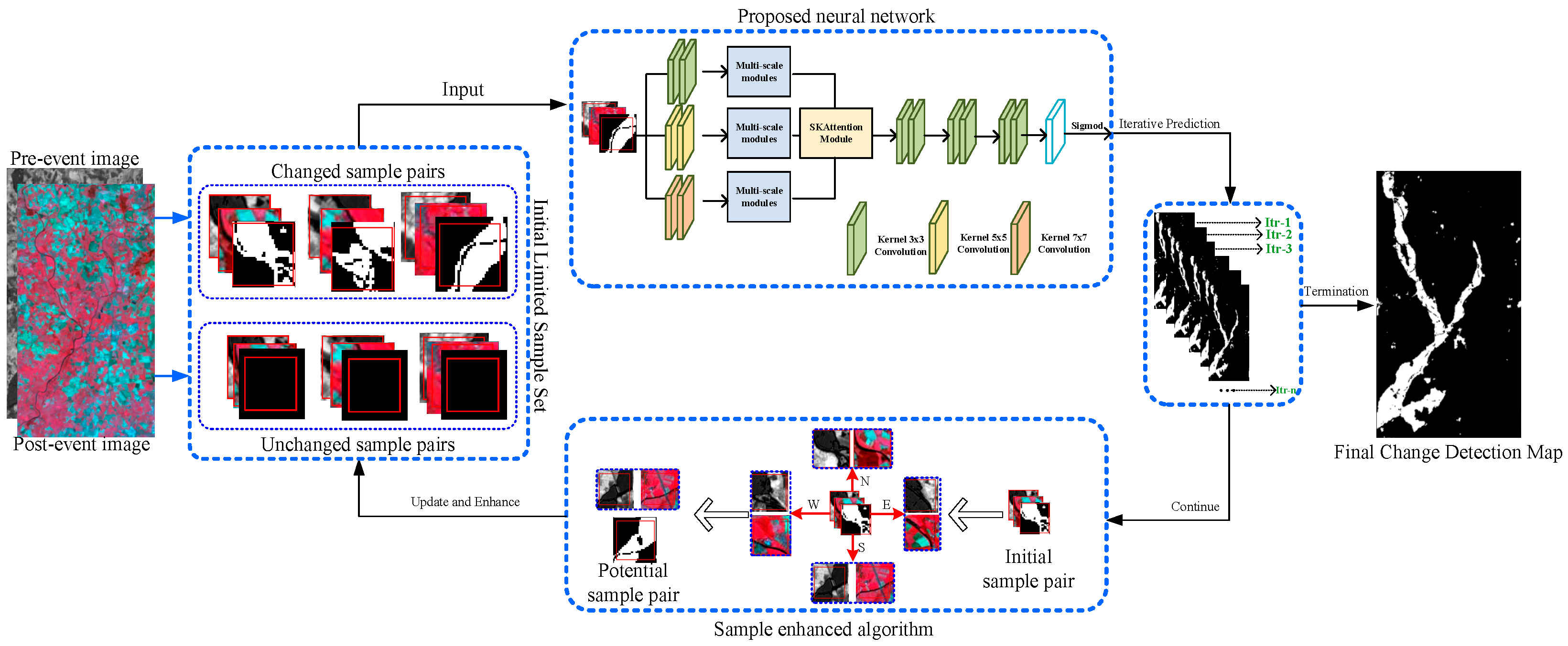
In this section, we provided a detailed description of the proposed framework for Hete-CD, including an overview and backbone of the proposed neural network, a non-parameter sample-enhanced algorithm, and an accuracy assessment. Every part is detailed in the following section. It is worth noting that the proposed approach was realized with the Pytorch 1.9 software, Python 3.8 was used for coding, the version of the OpenCV library is 4.6, and our code has been released on GitHub, which can be accessed by clicking on the link in the abstract section.

2.1. Overview

The motivation behind this study was to achieve change detection in Hete-CD with a limited number of samples. Accordingly, a novel framework was designed here to achieve the objective. Figure 1 depicts the flowchart of the proposed framework, which has four major parts, including an overview of the proposed approach, a proposed deep-learning neural network, a non-parameter sample-enhanced algorithm, and an accuracy assessment.
The overview of the proposed framework indicated that the framework iteratively generated a change detection map, and the final detection map was outputted when the iteration was terminated. The framework was initialized with a small number of samples, and the initial training sample set was amplified using a proposed nonparametric sample-enhanced algorithm in every iteration. The details of the termination condition of the proposed framework are presented in the following section.
To clarify this concept, the matched pixels for changed and unchanged classes between three adjacent iterations were defined in Equation (1) as follows:
M k 1 , k L M k , k + 1 L ε
M k 1 , k L = c o u n t ( M k 1 L M k L ) W × H
M k , k + 1 L = c o u n t ( M k L M k + 1 L ) W × H
where in L 0,1 , 0 and 1 denote the unchanged and changed classes, respectively. W and H denote the width and height of an input image. M k 1 , k L and M k , k + 1 L are the similarity measurements in terms of the k -th classification map and ( k 1 )th-classification map for the L-class, and they can be calculated by using Equations (2) and (3), respectively. “<—>” represents the matched pixels with the same label, including the changed and unchanged labels. For example, if the pairwise pixels at position (i,j) were marked with the “changed” or “unchanged” label in M k L and M k 1 L , then the pairwise pixels were defined as “matched”. Equation (1) demonstrated the similarity between the detection map from the (k − 1)th and kth and kth and (k + 1)th iterations. Moreover, ε was a small constant, and it was fixed at 0.0001 in our proposed framework. The training sample was dynamically adjusted in the iterative process. For example, if the change class satisfies Equation (1), then the corresponding changed sample will not be enhanced in the next iteration. Moreover, Equation (1) will be checked again in every iteration. Equation (1) indicated that the iteration of the proposed framework was terminated when the difference between the matched ratio among the (k − 1)th, kth, and (k + 1) detection maps was less than ε for the unchanged and changed classes.
In addition to the overview of the proposed framework, the two major parts were the proposed deep learning neural network and the non-parameter sample-enhanced algorithm. The details are presented as follows:

2.2. Proposed Deep-Learning Neural Network

Different ground targets were performed with varying sizes in remote sensing images, and distinguishing a target, such as a lake or a building, required an appropriate scale from the human visual perspective [59,60]. Accordingly, three aspects were considered in the proposed neural network, as shown in Figure 1. First, the bitemporal images were concatenated into one image and fed into three parallel branches. Each branch contained two convolution layers and one multiscale module. Every convolution layer in each branch had a different kernel size. The objective of this operation was to learn multiscale features for describing the various targets with different sizes. Second, a selective kernel (SK) attention module [61] was used to adaptively adjust its receptive field size based on multiple scales of the input information, with the aim of guiding the module to learn a selective scale for a specific target. After that, six convolutional layers with a 3 × 3 kernel size were used. The SK-attention was also utilized to smooth the detection noise further. Finally, the proposed neural network was activated by using the Sigmoid function.
The proposed neural network was trained with 20 epochs for one iteration in the entire framework and used to predict one change detection map. When the training samples were enhanced, the proposed neural network was trained again with the new sample set. During the training, a widely used loss function named cross-entropy was adopted, and a r g m a x ( · ) was utilized for prediction.

Non-Parameter Sample-Enhanced Algorithm

Labeling training samples is widely recognized to be time-consuming and labor-intensive, and a sufficient number of samples are required to train a deep learning model effectively [62]. Therefore, a non-parameter sample-enhanced algorithm was proposed and embedded in our proposed framework. The details of the sample-enhanced algorithm are presented as follows:
Here, X i j and Y i j represented the image blocks with 16 × 16 pixels of the pre-event and post-event, respectively. X i j and Y i j were defined as the known samples. The neighboring image blocks around the known sample position (i, j) were selected as the potential training samples. Every potential sample was overlapped by a quarter with the known sample. In this study, the correlation between X i j and Y i j was measured by the Pearson correlation coefficient (PCC), as follows:
P X i j , Y i j = E ( x i j μ x i j ) ( y i j μ y i j ) δ ( x i j ) δ ( y i j ) ,
where E ( · ) is an expectation; x i j and μ x i j represent the pixel within the spatial domain of X i j and the mean of these pixels in terms of gray value, respectively; σ ( · ) is the standard deviation of the pixels within X i j ; and P X i j , Y i j reflects the linear correlation between the pixels of the samples from the HRSIs. The label of the samples around the known sample pair X i j   Y i j is distinguished as follows based on the definition:
L S i j t 1 , S i j t 2 = 1 , i f   P S i j t 1 , S i j t 2 P 1 ( X i j , Y i j ) 0 , i f   P S i j t 1 , S i j t 2 P 0 ( X i j , Y i j ) ,
where L denotes the sample’s label; L = 1 and L = 0 denote the changed and unchanged classes. Therefore, P 1 ( · ) and P 0 ( · ) denote the correlation relationship similarity between the pairwise image blocks ( X i j and Y i j ) which are the known samples, and the central pixel of the known sample image blocks at the position (i, j) are the changed and unchanged labels. In addition, t 1 and t 2 denote the samples extracted from the bitemporal images that were acquired at date-t1 and date-t2, respectively. The defined rules indicated that when the label of the known sample was “changed” and if the correlation between the pairwise neighboring potential samples ( S i j t 1 and S i j t 2 ) was less than or equal to that of the known sample ( X i j and Y i j ), then the label of the pairwise neighboring potential sample will be marked as “changed”. By contrast, when the label of the known sample was “unchanged” and if L S i j t 1 , S i j t 2 P 0 ( X i j , Y i j ) , then the label of the pairwise neighboring potential sample will be marked as “unchanged”. Based on this definition, the initial sample set with a limited size was gradually amplified during the iteration, and the enhanced sample set was re-used to train the proposed neural network to generate the preferred detection performance.
These PCC-based rules were effective for investigating potential samples around each known sample with regard to the following intuitive assumptions: (1) PCC can measure the correlation between two datasets from different modalities; (2) Around a sample with a changed label, the lower correlation between pairwise heterogonous image blocks indicates a lower possibility of change between them; (3) Around a sample with an unchanged label, the higher correlation between the pairwise heterogonous image blocks indicates a higher possibility of change between them.

2.3. Accuracy Assessment

Nine widely used evaluation indicators are used in our study to investigate performance quantitatively. The details are summarized in Table 1. Here, four variables are defined to clarify the referred indicators: True positive (TP) refers to the number of accurately detected changed pixels; true negative (TN) is the number of accurately detected unchanged pixels; false positive (FP) is the number of inaccurately detected changed pixels; and false negative (FN) is the number of inaccurately detected unchanged pixels.

3. Experiments

Two experiments are designed here to verify the superiority and performance of our proposed framework for Hete-CD. The first experiment aims to compare the proposed approach with state-of-the-art methods with four pairs of real HRSIs to verify the feasibility and advantages of the proposed approach. The second experiment focused on revealing the relationship between the number of initial samples and the detection accuracy of the proposed approach. The experiments are performed on four pairs of actual HRSIs. The detailed descriptions of the experiments are presented in the following section.

3.1. Dataset Description

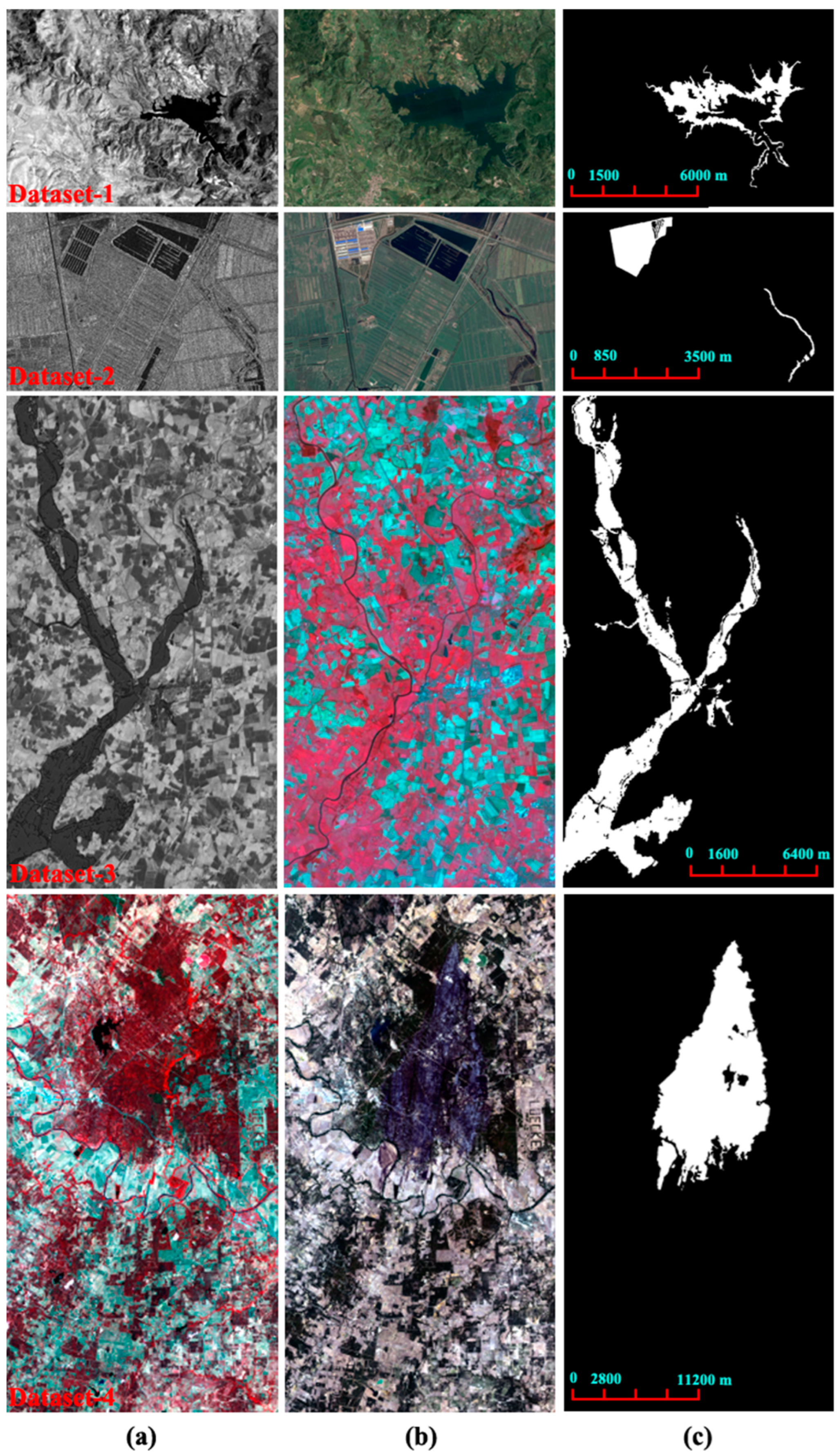
Four pairs of HRSIs are used for the experiments. In Figure 2, these images refer to water body change, building construction, floods, and wildfire change events. The image acquired before the occurrence of the change event is defined as a “pre-event image”. Meanwhile, the image acquired after the occurrence of the change event is defined as a “post-event image”. The details of each image pair are detailed as follows:
Dataset-1: This dataset contained different optical images acquired from various sources. The pre-event image was acquired by Landsat-5 in September 1995 and exhibited a size of 300 × 400 × 1 pixels with 30 m/pixel. The post-event image was acquired in July 1996 and clipped from Google Earth; its size was 300 × 400 × 3 pixels with 30 m/pixel. This type of pairwise HRSI was easily available. Here, these images were used to detect the expansion area of the Sarindia (Italy) Lake.
Dataset-2: This dataset contained a SAR pre-event image acquired with the Radarsat-2 satellite in June 2008 and an optical post-event image extracted from Google Earth in September 2012. The sizes of the HRSIs were 593 × 921 × 1 and 593 × 921 × 3 pixels with 8 m/pixel resolution. The change event was the building construction located in Shuguang Village, China.
Dataset-3: This dataset included SPOT Xs-ERS and SPOT images for the pre-event and post-event, respectively. The pre-event and post-event images were acquired in October 1999 and October 2000, before and after a flood over Gloucester, U.K. The size of these images was 990 × 554 pixels with a 15 m/pixel resolution. The pre-event image and post-event image have one and three bands, respectively. In particular, the ERS image reflected the roughness of the ground before the flood, and the multispectral SPOT HRV image described the color of the ground during the flood. The detection task aimed at calculating the change areas by comparing the bitemporal heterogonous images.
Dataset-4: This dataset contained two images acquired by using different sensors (Landsat-5 TM and Landsat-8) over Bastrop County, Texas, USA, for a wildfire event on 4 September 2011. The size of the bi-temporal images was 1534 × 808 × 3 pixels and 30 m/pixel. The modality difference between the bi-temporal images lay in the pre-event image, which was acquired by Landsat-5 and composed of 4–3–2 bands, and the post-event image, which was obtained by Landsat-8 and composed of 5–4–3 bands.
Furthermore, the pre-processing operations for each dataset, including radiation correction, resampling, and co-registration, have been achieved by the owner of the datasets. Dataset-1 to Dataset-4 are open-accessible datasets widely used for evaluating the performance of change detection with heterogeneous remote sensing images, and the pre-processing operations have been conducted before release. Additional details, including the acquiring platform and the preprocessing steps for the datasets, can be found in reference [20].

3.2. Experimental Setup

In the experiments, nine state-of-the-art change detection methods, including three traditional methods and six deep learning methods, were selected for comparison. The details are presented as follows:
(i)
In the first part of the experiments, the three relatively new and highly cited related methods were as follows: The first method, named adaptive graph and structure cycle consistency (AGSCC) (https://github.com/yulisun/AGSCC, accessed on 1 May 2023) [45], focused on exploring the shared structural features of the bitemporal HRSIs. The explored shared structural features were comparable for change detection. The second method, named graph-based image regression and MRF segmentation method (GIR-MRF) (https://github.com/yulisun/GIR-MRF, accessed on 1 May 2023) [50], aimed at learning the shared features via graph-based image regression. The third method, called the sparse constrained adaptive structure consistency-based method (SCASC) (https://github.com/yulisun/SCASC, accessed on 1 May 2023) [42], attempted to improve the adaptive structural extraction efficiency for Hete-CD. These studies [42,45,50] were typical in the field of change detection with HRSIs. Accordingly, these studies were adopted for comparison with our proposed framework. Based on the comparisons, the parameters of the selected methods [42,45,50] were the same as those used in the original studies. Twelve unchanged samples (six pairs) and changed samples (six pairs) were randomly selected from the ground reference map for framework initialization in our proposed framework.
(ii)
The second part of the experiments aimed at verifying the advantages and feasibility of the proposed framework while comparing it with some state-of-the-art deep learning methods. The first method, named fully convolutional Siamese difference (FC-Siam-diff) [28], was an extension of UNet. The second method, named crosswalk detection network (CDNet) [55], aimed at learning the change magnitude between the bitemporal images through a cross-convolution strategy. The experimental results based on four datasets clearly demonstrated the robustness and superiority of the proposed CDNet. The selected method, called feature difference convolutional neural network (FDCNN) [26], conducted convolutions on the feature difference map and obtained the binary change detection map. A deeply supervised image fusion network (DSIFN) [63] concentrated on exploring highly representative deep features of bi-temporal images through a fully convolutional two-stream architecture for LCCD with HRSIs. A cross-layer convolutional neural network (CLNet) was first proposed for LCCD with HRSIs to learn the correlation between the bi-temporal images at different features. The four experimental applications clearly demonstrated the superiority of the proposed approach [27]. In addition, a multiscale fully convolutional network (MFCN) was constructed for the ground land cover change area with various shapes and sizes [30]. The following parameters are set for each network: learning rate = 0.0001, batch size = 3, and epochs = 20. All the selected deep learning methods used the same training samples randomly clipped and extracted from the ground reference map to guarantee comparative fairness. Moreover, the quantity of training samples for the state-of-the-art deep learning methods is equal to the number of enhanced samples when the iteration of our proposed framework is terminated.
(iii)
The ratio between the training samples, validation samples, and testing samples was about 2:1:7. The number of initial samples for each approach and dataset was 12 pairs. The initial samples for each dataset were randomly obtained based on the ground reference.

3.3. Results

The experimental results of the four pairs of HRSIs were obtained according to the above-mentioned parameter setting. The details are as follows:
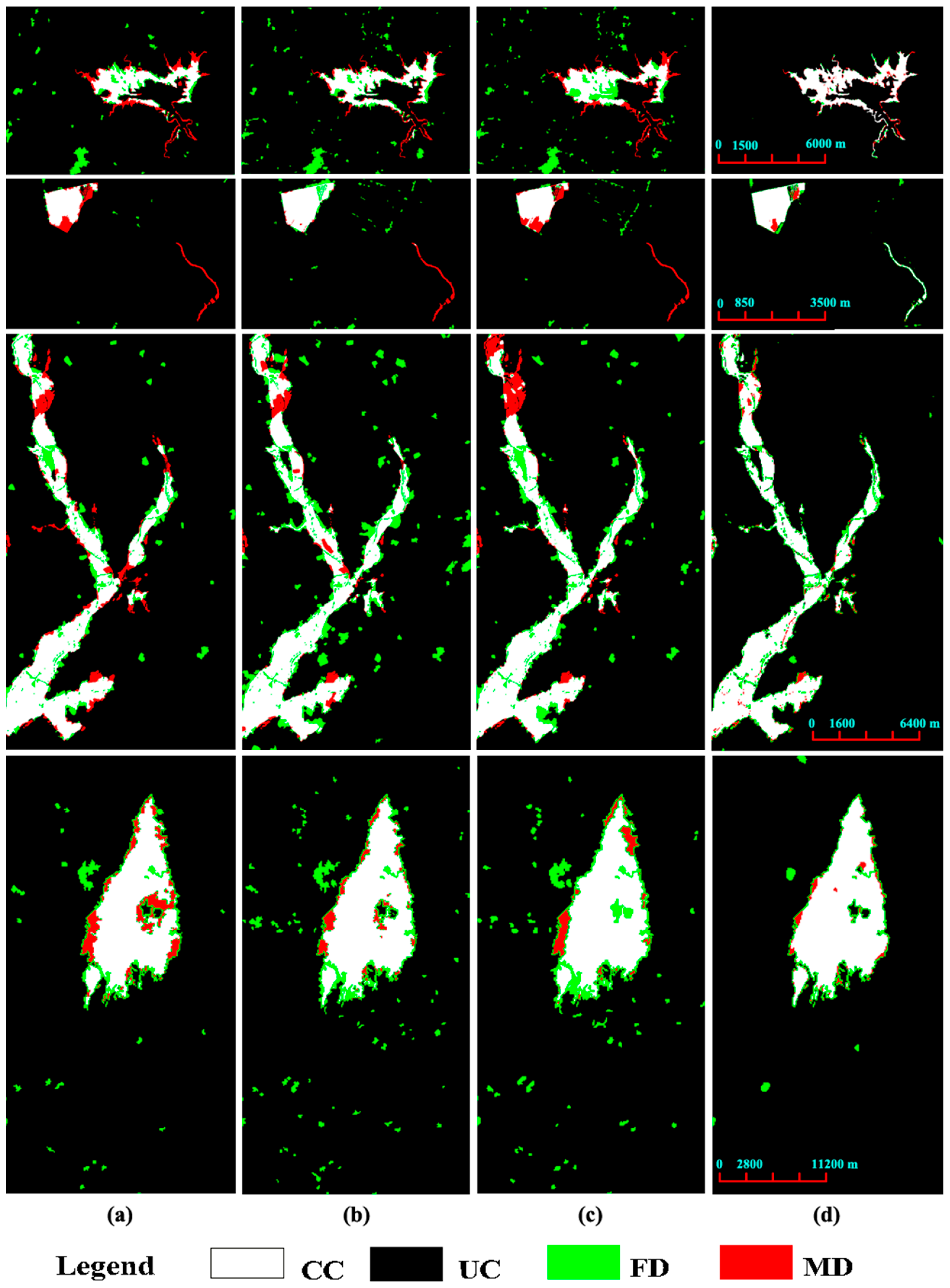
(i)
Comparisons with traditional methods: The visual performance of AGSCC [45], GIR-MRF [50], and SCASC [42] is presented in Figure 3a–c, respectively. In comparison with the results based on our proposed framework, Figure 3d shows that our proposed framework achieved the best detection performance with the fewest false alarm (green) and missed alarm (red) pixels. The corresponding quantitative results in Table 2 further supported the conclusion from the visual observation comparisons. For example, the proposed framework achieved 99.04%, 98.75%, 96.77%, and 97.92% in terms of OA for the four datasets. These values were the best among the results from AGSCC [45], GIR-MRF [50], SCASC [42], and our proposed framework.
(ii)
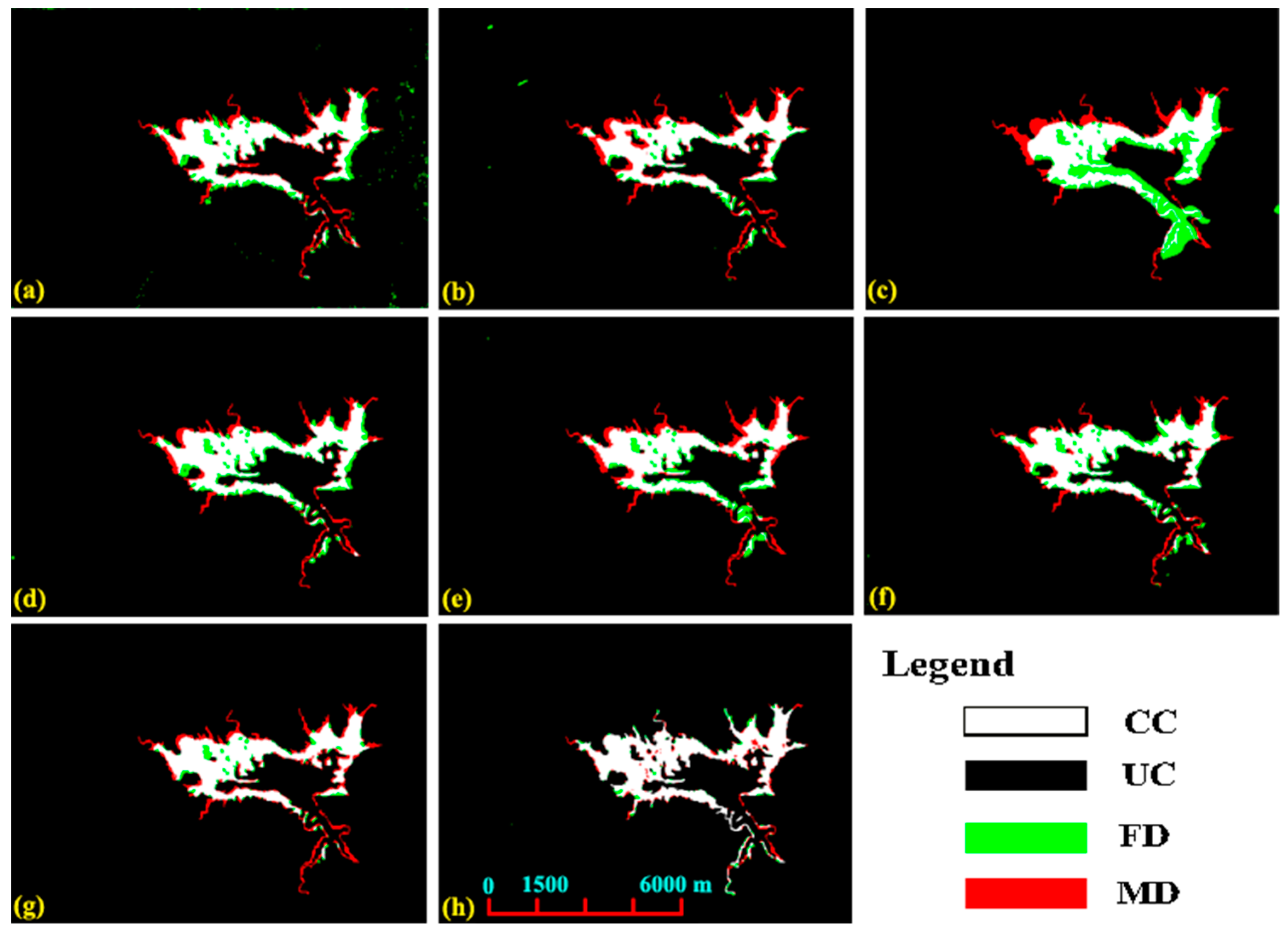
Comparisons with deep learning methods: We further verified the robustness of the proposed framework by comparing it with some state-of-the-art deep learning methods. The detection maps presented in Figure 4, Figure 5, Figure 6 and Figure 7 are acquired by using different deep-learning methods for the four datasets. These visual comparisons indicated that the proposed framework performed better with fewer false and missed alarms. During the removal of the sample-enhanced algorithm from the entire proposed framework, as denoted by “Proposed-” in Table 3, Table 4, Table 5 and Table 6, the improvement was achieved compared with that of the other approaches for the same datasets. For example, the proposed approach obtained the best OA = 99.04% and the based FA = 0.33%. In comparison with the results based on the proposed approach without the proposed sample enhancement approach, the improvement of the proposed approach coupled with the sample-enhanced algorithm was approximately 2.0% in terms of OA for Dataset-1. Multiscale information extraction and selective kernel attention in the promoted neural network were complementary to learning more accuracy in our proposed framework. The following quantitative comparisons in Table 3, Table 4, Table 5 and Table 6 further supported the visually observed conclusion.

3.4. Discussion

The novelty of the proposed approach lies in promoting a novel way to improve the change detection performance of LCCD with HRSIs. Accordingly, a novel sample augmentation algorithm for change detection with HRSIs was proposed to achieve this objective. The proposed approach allowed us to obtain a satisfactory change detection map with a small initial training sample set for practical applications. Here, two aspects of the training samples for the proposed framework are discussed and analyzed to promote further use and understanding of this framework, as follows:
(i)
Relationship between the initial and the final samples: According to Section 2, the proposed framework was initialized with a small number of training samples, which were iteratively amplified at every iteration. Accordingly, observing the relationship between the initial and final samples helps us understand the balancing ability for unchanged and changed classes in our proposed framework. Figure 8 shows that the quantity of samples for the changed and unchanged classes is equal for initialization. When the iteration of the proposed framework was terminated, the number of samples for the unchanged and changed classes was automatically adjusted to be different because the size of the area was distinct in an image scene. Detecting them with an unequal sample is beneficial for balancing their detection accuracies. Figure 8 also demonstrates that the relationship between the initial and final samples is nonlinear. For example, for the unchanged and changed samples of Dataset-1, when the initial samples for the unchanged class increased from three to four pairs, its final samples decreased from 56 pairs to 33 pairs. Moreover, different datasets exhibit the relationship between the initial and final samples for our proposed framework. Therefore, determining the suitable quantity of samples for initializing the proposed framework may involve conducting trial-and-error experiments in practical applications.
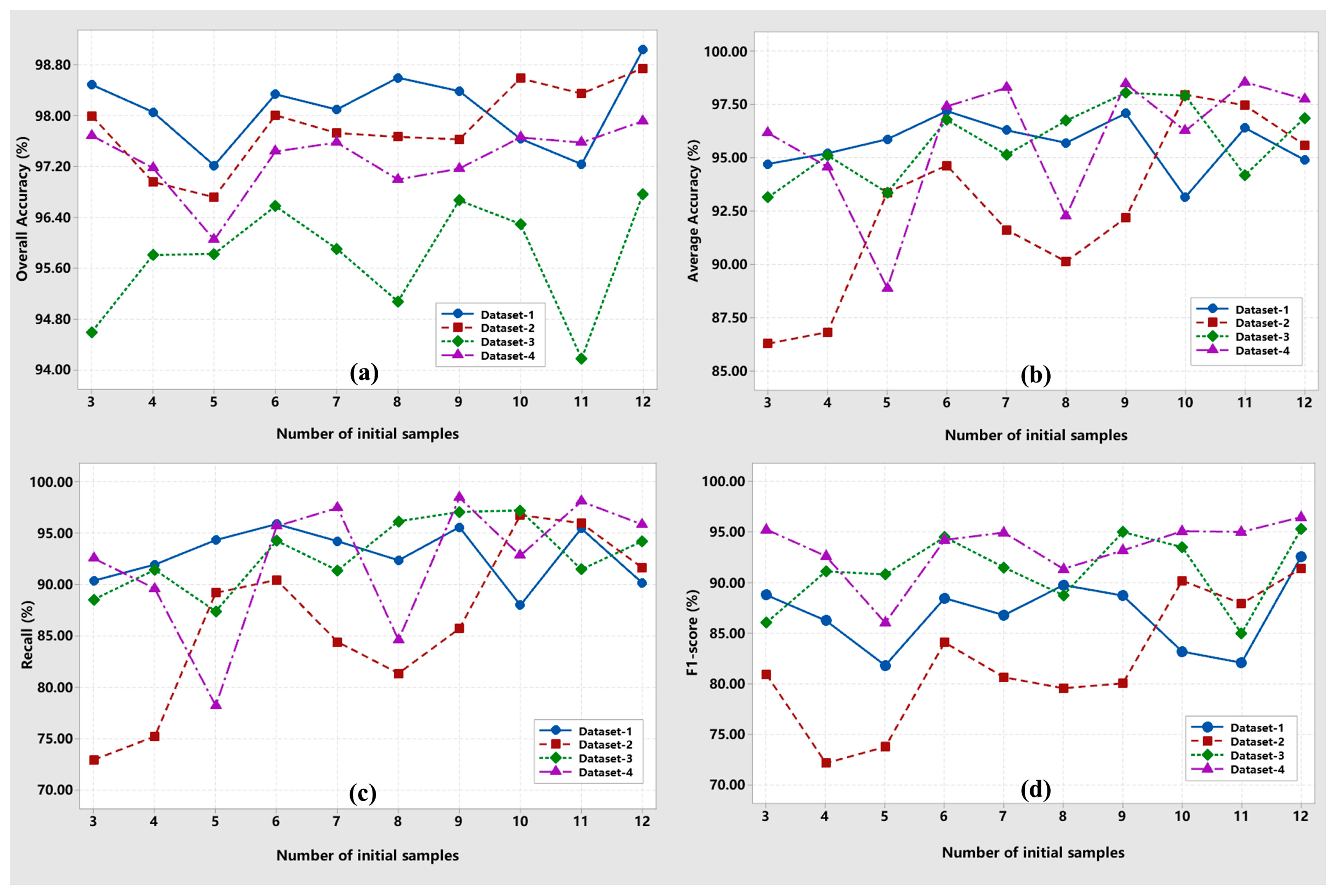
(ii)
Relationship between the initial samples and detection accuracies: The observation results indicated that the detection accuracy initially decreased with the increment of the initial samples for some datasets (Figure 9). Moreover, the accuracy increased and appeared to be a state with a small variation. For example, the OA for Dataset-2 and -4 decreased when the initial samples increased from three pairs to four pairs, and then it increased and vibrated within [96.72%, 98.75%] and [96.05%, 97.92%], respectively. Some explored samples may be marked with missed labels, which negatively affected the learning performance. However, the sample with missed labels becomes the minority in the total enhanced sample set with the increment of the initial training samples. Consequently, an uncertain relationship may cause detection accuracy variation when training our proposed framework with the sample set. The observation illustrated in Figure 9 indicates the proposed approach can explore samples. However, the detection accuracy did not always linearly improve with the number of samples. This phenomenon is due to the distinct variability, spectral homogeneity, and uncertainty of each dataset.

4. Conclusions

In this study, a novel deep learning-based framework is proposed to achieve change detection with heterogeneous remote sensing images when the training samples are limited. The result showed that improving detection accuracy via sample augmentation is feasible. The proposed framework is a combination of a novel multiscale neural network and a novel non-parameter sample-enhanced algorithm in iterative progress to achieve satisfactory detection performance with a small number of initial training samples. The advantages of the proposed framework are summarized as follows:
(i)
Advanced detection accuracy is obtained with the proposed framework. The comparative results with four pairs of actual HTRSIs indicated that the proposed framework outperforms three traditional cognate methods in terms of visual performance and nine quantitative evaluation metrics.
(ii)
Iteratively training deep learning neural networks with a non-parameter sample-enhanced algorithm is effective in improving detection performance with limited initial samples. This work is the first to combine a non-parameter sample-enhanced algorithm with a deep learning neural network for iteratively training the neural network with the enhanced training samples from every iteration. The experimental results and comparisons demonstrated the feasibility and effectiveness of the recommended sample-enhanced algorithm and training strategy for our proposed framework.
(iii)
A simple, robust, and non-parameter framework is preferred and acceptable for practical engineering applications. In addition to the small number of initial training samples for initialization, the proposed framework has no parameters that require hard tuning. This characteristic can be easily applied to practical engineering.
The Hete-CD aims at exploring the shared feature in multi-module images and measuring the change magnitude to achieve the land cover change detection task. It is an important supplement for change detection with homogeneous RSIs and proposes an approach that is robust to various datasets and that is preferred for practical applications.
Although the proposed framework offers some advantages and may be helpful for any other classification and land use application with remote sensing images, the widespread application with large areas and other types of change events should be further investigated. In our future study, we will focus on collecting more types of HTRSIs, and multiclass change detection will be considered.

Author Contributions

Y.Z. was primarily responsible for the original idea and the experimental design. Q.L. performed the experiments. Z.L. provided ideas to improve the quality of the paper. N.F. supervised and revised the language of this work. All authors have read and agreed to the published version of the manuscript.

Funding

This work was financially supported by the Shaanxi Provincial Department of Science and Technology Fund Project “Shaanxi Provincial Innovation Capability Support Program” (No. 2021PT-009).

Acknowledgments

The authors thank the editor-in-chief, associate editor, and reviewers for their insightful comments and suggestions.

Conflicts of Interest

The authors declare no conflict of interest.

References

  1. Singh, A. Review article digital change detection techniques using remotely-sensed data. Int. J. Remote Sens. 1989, 10, 989–1003. [Google Scholar] [CrossRef]
  2. Pande, C.B. Land use/land cover and change detection mapping in Rahuri watershed area (MS), India using the google earth engine and machine learning approach. Geocarto Int. 2022, 37, 13860–13880. [Google Scholar] [CrossRef]
  3. Lv, Z.; Huang, H.; Sun, W.; Jia, M.; Benediktsson, J.A.; Chen, F. Iterative Training Sample Augmentation for Enhancing Land Cover Change Detection Performance With Deep Learning Neural Network. IEEE Trans. Neural Netw. Learn. Syst. 2023, 1–14. [Google Scholar] [CrossRef]
  4. Anniballe, R.; Noto, F.; Scalia, T.; Bignami, C.; Stramondo, S.; Chini, M.; Pierdicca, N. Earthquake damage mapping: An overall assessment of ground surveys and VHR image change detection after L’Aquila 2009 earthquake. Remote Sens. Environ. 2018, 210, 166–178. [Google Scholar] [CrossRef]
  5. Li, Z.; Shi, W.; Lu, P.; Yan, L.; Wang, Q.; Miao, Z. Landslide mapping from aerial photographs using change detection-based Markov random field. Remote Sens. Environ. 2016, 187, 76–90. [Google Scholar] [CrossRef]
  6. Li, Z.; Shi, W.; Myint, S.W.; Lu, P.; Wang, Q. Semi-automated landslide inventory mapping from bitemporal aerial photographs using change detection and level set method. Remote Sens. Environ. 2016, 175, 215–230. [Google Scholar] [CrossRef]
  7. Bouziani, M.; Goïta, K.; He, D.-C. Automatic change detection of buildings in urban environment from very high spatial resolution images using existing geodatabase and prior knowledge. ISPRS J. Photogramm. Remote Sens. 2010, 65, 143–153. [Google Scholar] [CrossRef]
  8. Coppin, P.; Jonckheere, I.; Nackaerts, K.; Muys, B.; Lambin, E. Review ArticleDigital change detection methods in ecosystem monitoring: A review. Int. J. Remote Sens. 2004, 25, 1565–1596. [Google Scholar] [CrossRef]
  9. Leichtle, T.; Geiß, C.; Wurm, M.; Lakes, T.; Taubenböck, H. Unsupervised change detection in VHR remote sensing imagery–an object-based clustering approach in a dynamic urban environment. Int. J. Appl. Earth Obs. Geoinf. 2017, 54, 15–27. [Google Scholar] [CrossRef]
  10. Munyati, C. Wetland change detection on the Kafue Flats, Zambia, by classification of a multitemporal remote sensing image dataset. Int. J. Remote Sens. 2000, 21, 1787–1806. [Google Scholar] [CrossRef]
  11. Xian, G.; Homer, C.; Fry, J. Updating the 2001 National Land Cover Database land cover classification to 2006 by using Landsat imagery change detection methods. Remote Sens. Environ. 2009, 113, 1133–1147. [Google Scholar] [CrossRef]
  12. Gao, J.; Liu, Y. Determination of land degradation causes in Tongyu County, Northeast China via land cover change detection. Int. J. Appl. Earth Obs. Geoinf. 2010, 12, 9–16. [Google Scholar] [CrossRef]
  13. Taubenböck, H.; Esch, T.; Felbier, A.; Wiesner, M.; Roth, A.; Dech, S. Monitoring urbanization in mega cities from space. Remote Sens. Environ. 2012, 117, 162–176. [Google Scholar] [CrossRef]
  14. Zhang, T.; Huang, X. Monitoring of urban impervious surfaces using time series of high-resolution remote sensing images in rapidly urbanized areas: A case study of Shenzhen. IEEE J. Sel. Top. Appl. Earth Obs. Remote Sens. 2018, 11, 2692–2708. [Google Scholar] [CrossRef]
  15. Awad, M.M. An innovative intelligent system based on remote sensing and mathematical models for improving crop yield estimation. Inf. Process. Agric. 2019, 6, 316–325. [Google Scholar] [CrossRef]
  16. Lv, Z.; Liu, T.; Benediktsson, J.A.; Falco, N. Land cover change detection techniques: Very-high-resolution optical images: A review. IEEE Geosci. Remote Sens. Mag. 2021, 10, 44–63. [Google Scholar] [CrossRef]
  17. Zhu, Z. Change detection using landsat time series: A review of frequencies, preprocessing, algorithms, and applications. ISPRS J. Photogramm. Remote Sens. 2017, 130, 370–384. [Google Scholar] [CrossRef]
  18. Hachicha, S.; Chaabane, F. On the SAR change detection review and optimal decision. Int. J. Remote Sens. 2014, 35, 1693–1714. [Google Scholar] [CrossRef]
  19. Wen, D.; Huang, X.; Bovolo, F.; Li, J.; Ke, X.; Zhang, A.; Benediktsson, J.A. Change detection from very-high-spatial-resolution optical remote sensing images: Methods, applications, and future directions. IEEE Geosci. Remote Sens. Mag. 2021, 9, 68–101. [Google Scholar] [CrossRef]
  20. Lv, Z.; Huang, H.; Li, X.; Zhao, M.; Benediktsson, J.A.; Sun, W.; Falco, N. Land cover change detection with heterogeneous remote sensing images: Review, progress, and perspective. Proc. IEEE 2022, 110, 1976–1991. [Google Scholar] [CrossRef]
  21. Hong, S.; Vatsavai, R.R. Sliding window-based probabilistic change detection for remote-sensed images. Procedia Comput. Sci. 2016, 80, 2348–2352. [Google Scholar] [CrossRef]
  22. Lu, P.; Qin, Y.; Li, Z.; Mondini, A.C.; Casagli, N. Landslide mapping from multi-sensor data through improved change detection-based Markov random field. Remote Sens. Environ. 2019, 231, 111235. [Google Scholar] [CrossRef]
  23. Lv, Z.; Liu, T.; Shi, C.; Benediktsson, J.A. Local histogram-based analysis for detecting land cover change using VHR remote sensing images. IEEE Geosci. Remote Sens. Lett. 2020, 18, 1284–1287. [Google Scholar] [CrossRef]
  24. Chen, L.; Liu, C.; Chang, F.; Li, S.; Nie, Z. Adaptive multi-level feature fusion and attention-based network for arbitrary-oriented object detection in remote sensing imagery. Neurocomputing 2021, 451, 67–80. [Google Scholar] [CrossRef]
  25. Mou, L.; Bruzzone, L.; Zhu, X.X. Learning spectral-spatial-temporal features via a recurrent convolutional neural network for change detection in multispectral imagery. IEEE Trans. Geosci. Remote Sens. 2018, 57, 924–935. [Google Scholar] [CrossRef]
  26. Zhang, M.; Shi, W. A feature difference convolutional neural network-based change detection method. IEEE Trans. Geosci. Remote Sens. 2020, 58, 7232–7246. [Google Scholar] [CrossRef]
  27. Zheng, Z.; Wan, Y.; Zhang, Y.; Xiang, S.; Peng, D.; Zhang, B. CLNet: Cross-layer convolutional neural network for change detection in optical remote sensing imagery. ISPRS J. Photogramm. Remote Sens. 2021, 175, 247–267. [Google Scholar] [CrossRef]
  28. Daudt, R.C.; Le Saux, B.; Boulch, A. Fully convolutional siamese networks for change detection. In Proceedings of the 2018 25th IEEE International Conference on Image Processing (ICIP), Athens, Greece, 7–10 October 2018; pp. 4063–4067. [Google Scholar]
  29. Chen, J.; Yuan, Z.; Peng, J.; Chen, L.; Huang, H.; Zhu, J.; Liu, Y.; Li, H. DASNet: Dual attentive fully convolutional Siamese networks for change detection in high-resolution satellite images. IEEE J. Sel. Top. Appl. Earth Obs. Remote Sens. 2020, 14, 1194–1206. [Google Scholar] [CrossRef]
  30. Li, X.; He, M.; Li, H.; Shen, H. A combined loss-based multiscale fully convolutional network for high-resolution remote sensing image change detection. IEEE Geosci. Remote Sens. Lett. 2021, 19, 8017505. [Google Scholar] [CrossRef]
  31. Huang, R.; Zhou, M.; Zhao, Q.; Zou, Y. Change detection with absolute difference of multiscale deep features. Neurocomputing 2020, 418, 102–113. [Google Scholar] [CrossRef]
  32. Chen, P.; Li, C.; Zhang, B.; Chen, Z.; Yang, X.; Lu, K.; Zhuang, L. A Region-Based Feature Fusion Network for VHR Image Change Detection. Remote Sens. 2022, 14, 5577. [Google Scholar] [CrossRef]
  33. Asokan, A.; Anitha, J.; Patrut, B.; Danciulescu, D.; Hemanth, D.J. Deep feature extraction and feature fusion for bi-temporal satellite image classification. Comput. Mater. Contin. 2021, 66, 373–388. [Google Scholar] [CrossRef]
  34. Zhang, Z.-D.; Tan, M.-L.; Lan, Z.-C.; Liu, H.-C.; Pei, L.; Yu, W.-X. CDNet: A real-time and robust crosswalk detection network on Jetson nano based on YOLOv5. Neural Comput. Appl. 2022, 34, 10719–10730. [Google Scholar] [CrossRef]
  35. Yang, B.; Qin, L.; Liu, J.; Liu, X. UTRNet: An Unsupervised Time-Distance-Guided Convolutional Recurrent Network for Change Detection in Irregularly Collected Images. IEEE Trans. Geosci. Remote Sens. 2022, 60, 4410516. [Google Scholar] [CrossRef]
  36. Fiorucci, F.; Giordan, D.; Santangelo, M.; Dutto, F.; Rossi, M.; Guzzetti, F. Criteria for the optimal selection of remote sensing optical images to map event landslides. Nat. Hazards Earth Syst. Sci. 2018, 18, 405–417. [Google Scholar] [CrossRef]
  37. Huang, Z.; Zhang, Y.; Li, Q.; Zhang, T.; Sang, N.; Hong, H. Progressive dual-domain filter for enhancing and denoising optical remote-sensing images. IEEE Geosci. Remote Sens. Lett. 2018, 15, 759–763. [Google Scholar] [CrossRef]
  38. You, Y.; Cao, J.; Zhou, W. A survey of change detection methods based on remote sensing images for multi-source and multi-objective scenarios. Remote Sens. 2020, 12, 2460. [Google Scholar] [CrossRef]
  39. Gong, M.; Jiang, F.; Qin, A.K.; Liu, T.; Zhan, T.; Lu, D.; Zheng, H.; Zhang, M. A spectral and spatial attention network for change detection in hyperspectral images. IEEE Trans. Geosci. Remote Sens. 2021, 60, 5521614. [Google Scholar] [CrossRef]
  40. Wan, L.; Zhang, T.; You, H. Multi-sensor remote sensing image change detection based on sorted histograms. Int. J. Remote Sens. 2018, 39, 3753–3775. [Google Scholar] [CrossRef]
  41. Lei, L.; Sun, Y.; Kuang, G. Adaptive local structure consistency-based heterogeneous remote sensing change detection. IEEE Geosci. Remote Sens. Lett. 2020, 19, 8003905. [Google Scholar] [CrossRef]
  42. Sun, Y.; Lei, L.; Guan, D.; Li, M.; Kuang, G. Sparse-Constrained Adaptive Structure Consistency-Based Unsupervised Image Regression for Heterogeneous Remote-Sensing Change Detection. IEEE Trans. Geosci. Remote Sens. 2021, 60, 4405814. [Google Scholar] [CrossRef]
  43. Luppino, L.T.; Bianchi, F.M.; Moser, G.; Anfinsen, S.N. Unsupervised image regression for heterogeneous change detection. arXiv 2019, arXiv:1909.05948. [Google Scholar] [CrossRef]
  44. Luppino, L.T.; Bianchi, F.M.; Moser, G.; Anfinsen, S.N. Remote sensing image regression for heterogeneous change detection. In Proceedings of the 2018 IEEE 28th International Workshop on Machine Learning for Signal Processing (MLSP), Aalborg, Denmark, 17–20 September 2018; pp. 1–6. [Google Scholar]
  45. Sun, Y.; Lei, L.; Guan, D.; Wu, J.; Kuang, G.; Liu, L. Image regression with structure cycle consistency for heterogeneous change detection. IEEE Trans. Neural Netw. Learn. Syst. 2022, 1–15. [Google Scholar] [CrossRef] [PubMed]
  46. Wu, J.; Li, B.; Qin, Y.; Ni, W.; Zhang, H.; Sun, Y. A Multiscale Graph Convolutional Network for Change Detection in Homogeneous and Heterogeneous Remote Sensing Images. arXiv 2021, arXiv:2102.08041. [Google Scholar] [CrossRef]
  47. Sun, Y.; Lei, L.; Li, X.; Tan, X.; Kuang, G. Patch Similarity Graph Matrix-Based Unsupervised Remote Sensing Change Detection With Homogeneous and Heterogeneous Sensors. IEEE Trans. Geosci. Remote Sens. 2021, 59, 4841–4861. [Google Scholar] [CrossRef]
  48. Sun, Y.; Lei, L.; Li, X.; Tan, X.; Kuang, G. Structure Consistency-Based Graph for Unsupervised Change Detection With Homogeneous and Heterogeneous Remote Sensing Images. IEEE Trans. Geosci. Remote Sens. 2021, 60, 4700221. [Google Scholar] [CrossRef]
  49. Sun, Y.; Lei, L.; Guan, D.; Kuang, G. Iterative Robust Graph for Unsupervised Change Detection of Heterogeneous Remote Sensing Images. IEEE Trans. Image Process. 2021, 30, 6277–6291. [Google Scholar] [CrossRef]
  50. Sun, Y.; Lei, L.; Tan, X.; Guan, D.; Wu, J.; Kuang, G. Structured graph based image regression for unsupervised multimodal change detection. ISPRS J. Photogramm. Remote Sens. 2022, 185, 16–31. [Google Scholar] [CrossRef]
  51. Liu, Z.; Li, G.; Mercier, G.; He, Y.; Pan, Q. Change detection in heterogenous remote sensing images via homogeneous pixel transformation. IEEE Trans. Image Process. 2017, 27, 1822–1834. [Google Scholar] [CrossRef]
  52. Lv, Z.; Zhang, P.; Sun, W.; Benediktsson, J.A.; Li, J.; Wang, W. Novel Adaptive Region Spectral-Spatial Features for Land Cover Classification with High Spatial Resolution Remotely Sensed Imagery. IEEE Trans. Geosci. Remote Sens. 2023, 61, 5609412. [Google Scholar] [CrossRef]
  53. Lv, Z.; Zhong, P.; Wang, W.; You, Z.; Shi, C. Novel Piecewise Distance based on Adaptive Region Key-points Extraction for LCCD with VHR Remote Sensing Images. IEEE Trans. Geosci. Remote Sens. 2023, 61, 5607709. [Google Scholar] [CrossRef]
  54. Guo, Y.; Liu, Y.; Oerlemans, A.; Lao, S.; Wu, S.; Lew, M.S. Deep learning for visual understanding: A review. Neurocomputing 2016, 187, 27–48. [Google Scholar] [CrossRef]
  55. Lv, Z.; Zhong, P.; Wang, W.; You, Z.; Falco, N. Multi-scale Attention Network Guided with Change Gradient Image for Land Cover Change Detection Using Remote Sensing Images. IEEE Geosci. Remote Sens. Lett. 2023, 20, 2501805. [Google Scholar] [CrossRef]
  56. Zhan, T.; Gong, M.; Jiang, X.; Li, S. Log-based transformation feature learning for change detection in heterogeneous images. IEEE Geosci. Remote Sens. Lett. 2018, 15, 1352–1356. [Google Scholar] [CrossRef]
  57. Wu, Y.; Li, J.; Yuan, Y.; Qin, A.; Miao, Q.-G.; Gong, M.-G. Commonality autoencoder: Learning common features for change detection from heterogeneous images. IEEE Trans. Neural Netw. Learn. Syst. 2021, 33, 4257–4270. [Google Scholar] [CrossRef]
  58. Niu, X.; Gong, M.; Zhan, T.; Yang, Y. A conditional adversarial network for change detection in heterogeneous images. IEEE Geosci. Remote Sens. Lett. 2018, 16, 45–49. [Google Scholar] [CrossRef]
  59. Zou, Z.; Shi, Z. Random access memories: A new paradigm for target detection in high resolution aerial remote sensing images. IEEE Trans. Image Process. 2017, 27, 1100–1111. [Google Scholar] [CrossRef]
  60. Li, Z.; You, Y.; Liu, F. Multi-scale ships detection in high-resolution remote sensing image via saliency-based region convolutional neural network. In Proceedings of the IGARSS 2019–2019 IEEE International Geoscience and Remote Sensing Symposium, Yokohama, Japan, 28 July–2 August 2019; pp. 246–249. [Google Scholar]
  61. Li, X.; Wang, W.; Hu, X.; Yang, J. Selective kernel networks. In Proceedings of the IEEE/CVF Conference on Computer Vision and Pattern Recognition, Long Beach, CA, USA, 15–20 June 2019; pp. 510–519. [Google Scholar]
  62. Balki, I.; Amirabadi, A.; Levman, J.; Martel, A.L.; Emersic, Z.; Meden, B.; Garcia-Pedrero, A.; Ramirez, S.C.; Kong, D.; Moody, A.R.; et al. Sample-size determination methodologies for machine learning in medical imaging research: A systematic review. Can. Assoc. Radiol. J. 2019, 70, 344–353. [Google Scholar] [CrossRef]
  63. Zhang, C.; Yue, P.; Tapete, D.; Jiang, L.; Shangguan, B.; Huang, L.; Liu, G. A deeply supervised image fusion network for change detection in high resolution bi-temporal remote sensing images. ISPRS J. Photogramm. Remote Sens. 2020, 166, 183–200. [Google Scholar] [CrossRef]
Figure 1. Flowchart of the proposed framework for Hete-CD.
Remotesensing 15 04609 g001
Figure 2. Dataset-1 to -4: (a) Pre-event image, (b) post-even image, and (c) ground reference map.
Remotesensing 15 04609 g002
Figure 3. Comparison of the change detection visual performance of some state-of-the-art methods: (a) AGSCC [45], (b) GIR-MRF [50], (c) SCASC [42], (d) proposed framework (CC: accurately changed, UC: unchanged, FD: false detection, and MD: missed detection).
Remotesensing 15 04609 g003
Figure 4. Detection maps acquired by using different deep learning approaches for #1-Dataset: (a) FC-Siam-diff [28], (b) CDNet [34], (c) FDCNN [26], (d) DSIFN [63], (e) CLNet [27], (f) MFCN [30], (g) proposed-, and (h) proposed (CC: correctly changed, UC: unchanged, FD: false detection, and MD: missed detection).
Remotesensing 15 04609 g004
Figure 5. Detection maps acquired by using different deep learning approaches for #2-Dataset: (a) FC-Siam-diff [28], (b) CDNet [34], (c) FDCNN [26], (d) DSIFN [63], (e) CLNet [27], (f) MFCN [30], (g) proposed-, and (h) proposed (CC: correctly changed, UC: unchanged, FD: false detection, and MD: missed detection).
Remotesensing 15 04609 g005
Figure 6. Detection maps acquired by using different deep learning approaches for #3-Dataset: (a) FC-Siam-diff [28], (b) CDNet [34], (c) FDCNN [26], (d) DSIFN [63], (e) CLNet [27], (f) MFCN [30], (g) proposed-, and (h) proposed (CC: correctly changed, UC: unchanged, FD: false detection, and MD: missed detection).
Remotesensing 15 04609 g006
Figure 7. Detection maps acquired by using different deep learning approaches for #4-Dataset: (a) FC-Siam-diff [28], (b) CDNet [34], (c) FDCNN [26], (d) DSIFN [63], (e) CLNet [27], (f) MFCN [30], (g) proposed-, and (h) proposed (CC: correctly changed, UC: unchanged, FD: false detection, and MD: missed detection).
Remotesensing 15 04609 g007
Figure 8. Relationship between the initial and final samples at the end of the iteration for the proposed framework: (a) Dataset-1, (b) Dataset-2, (c) Dataset-3, and (d) Dataset-4.
Remotesensing 15 04609 g008
Figure 9. Relationship between the initial samples and the detection accuracies for the proposed framework: (a) Overall accuracy; (b) Average accuracy; (c) Recall, and (d) F1-score.
Remotesensing 15 04609 g009
Table 1. Quantitative accuracy evaluation indicators for each experiment.
Evaluation IndicatorsFormulaDefinition
False alarm (FA) F A = F P T N   +   F P FA is the ratio between the falsely changed and unchanged pixels of the ground truth.
Missed alarm (MA) M A = F N T P   +   F N MA is the ratio between the falsely unchanged and changed pixels of the ground truth.
Total error (TE) T E = F P   +   F N T P   +   T N   +   F P   +   F N TE is the ratio between the summary of falsely changed and unchanged pixels and the total pixels of the ground map.
Overall accuracy (OA) O A = T P   +   T N T P   +   T N   +   F P   +   F N OA is the accurately detected pixels between the total pixels of the ground map.
Average accuracy (AA) A A = T P T P   +   F N + T N T N   +   F P / 2 AA is the mean of accurately detected changes and accurately unchanged ratios.
Kappa coefficient (Ka) P 0 = T P   +   T N T P   +   T N   +   F P   +   F N
P e = T P   +   F P   ×   T P   +   F N   +   ( F N   +   T N )   ×   ( F P   +   T N ) ( T P   +   T N   +   F P   +   F N ) 2
K a = P 0     P e 1     P e
Ka reflects the reliability of the detection map by measuring inter-rater reliability for the changed and unchanged classes.
Precision (Pr) P r = T P T P   +   F P Pr is the ratio between the accurately detected and total changed pixels in a detention map.
Recall (Re) R e = T P T P   +   F N Re is the ratio between the accurately detected and total changed pixels in the ground truth map.
F1-score (F1) F 1 = 2 × p r e c i s i o n   ×   r e c a l l p r e c i s i o n   +   r e c a l l F1 is the harmonic mean of precision and recall.
Table 2. Quantitative comparison between the three traditional methods and our proposed framework for Hete-CD with four actual datasets.
DatasetMethodsOAKappaAAFAMATEPrecisionRecallF-Score
Dataset-1AGSCC [45]95.660.6684.082.57529.264.34166.0770.7468.33
GIR-MRF [50]95.430.674688.343.49219.834.57361.9580.1769.89
SCASC [42]94.380.59583.413.95129.235.62455.9470.7762.49
Proposed framework99.040.920194.90.339.8610.96495.0490.1492.52
Dataset-2AGSCC [45]98.240.773283.030.282432.061.7692.1467.9478.21
GIR-MRF [50]98.180.8192.581.2513.601.8277.1886.4081.53
SCASC [42]97.90.74183.840.655431.672.09783.5668.3375.18
Proposed framework98.750.909795.60.41299.3920.76291.1391.6191.37
Dataset-3AGSCC [45]95.330.790490.733.16515.374.66978.9884.6381.71
GIR-MRF [50]93.60.738691.845.82410.56.468.3589.577.51
SCASC [42]94.750.770490.773.95214.55.25275.2585.580.05
Proposed framework96.770.946696.870.46025.8051.04996.3694.295.27
Dataset-4AGSCC [45]95.810.865291.380.750416.52.29792.683.587.81
GIR-MRF [50]95.80.88895.161.3778.3052.03788.2991.789.96
SCASC [42]95.270.905895.090.88238.9311.63391.9691.0791.51
Proposed framework97.920.960797.750.32724.1680.71397.1195.8396.47
Table 3. Quantitative comparison among the different methods for Dataset-1.
MethodsOAKappaAAFAMATEPrecisionRecallF-Score
FC-Siam-diff [28]97.050.760387.791.5322.902.9578.1277.1077.61
CDNet [34]97.370.768785.290.7828.642.6386.6171.3678.25
FDCNN [26]95.360.665887.423.4321.734.6461.7878.2769.05
DSIFN [63]97.300.780788.911.4220.762.7079.8079.2479.52
CLNet [27]97.110.755386.021.1926.762.8981.3173.2477.06
MFCN [30]97.410.792189.971.4618.592.5979.8181.4180.60
Proposed-97.830.80887.000.5225.482.1791.0274.5281.95
Proposed99.040.920194.90.339.8610.96495.0490.1492.52
Table 4. Quantitative comparison among the different methods for Dataset-2.
MethodsOAKappaAAFAMATEPrecisionRecallF-Score
FC-Siam-diff [28]97.050.637875.800.3748.032.4786.6851.9764.98
CDNet [34]97.320.84593.160.7712.911.2683.3287.0985.16
FDCNN [26]94.580.630893.073.999.874.2051.0290.1365.16
DSIFN [63]97.510.789383.900.1132.101.3796.2367.9079.62
CLNet [27] 97.950.819587.590.3324.491.3691.2975.5182.66
MFCN [30]97.650.790991.991.2814.731.8775.4885.2780.08
Proposed-98.120.80784.760.0630.421.4098.1069.5881.41
Proposed98.750.909795.60.41299.3920.76291.1391.6191.37
Table 5. Quantitative comparison among the different methods for Dataset-3.
MethodsOAKappaAAFAMATEPrecisionRecallF-Score
FC-Siam-diff [28]92.250.765795.856.152.165.5767.3197.8479.76
CDNet [34]93.620.861892.281.2014.232.5189.5985.7787.64
FDCNN [26]94.640.908198.282.051.391.9186.1098.6191.93
DSIFN [63]93.460.892698.482.630.402.2783.1199.6090.61
CLNet [27]89.740.661884.044.1027.836.3767.7672.1769.90
MFCN [30]95.870.896292.360.3114.971.9597.2685.0390.73
Proposed-95.880.903395.451.217.891.9390.8092.1191.45
Proposed96.770.946696.870.46025.8051.04996.3694.295.27
Table 6. Quantitative comparison among the different methods for Dataset-4.
MethodsOAKappaAAFAMATEPrecisionRecallF-Score
FC-Siam-diff [28]86.670.528286.74 11.84 14.68 11.97 45.30 85.32 59.18
CDNet [34]96.210.912693.27 0.18 13.29 1.39 98.06 86.71 92.03
FDCNN [26]94.880.854195.00 2.25 7.76 2.74 82.28 92.24 86.97
DSIFN [63]96.820.947697.24 0.48 5.03 0.91 95.59 94.97 95.28
CLNet [27]92.380.54270.03 0.1159.83 6.07 97.57 40.17 56.91
MFCN [30]97.50.937296.55 0.56 6.34 1.14 95.09 93.66 94.37
Proposed-97.750.950896.87 0.32 5.95 0.88 97.17 94.05 95.58
Proposed97.920.960797.750.334.1680.71397.1195.8396.47
Disclaimer/Publisher’s Note: The statements, opinions and data contained in all publications are solely those of the individual author(s) and contributor(s) and not of MDPI and/or the editor(s). MDPI and/or the editor(s) disclaim responsibility for any injury to people or property resulting from any ideas, methods, instructions or products referred to in the content.

