
Machine Learning-Based Estimation of Hourly GNSS Precipitable Water Vapour

Abstract
:1. Introduction
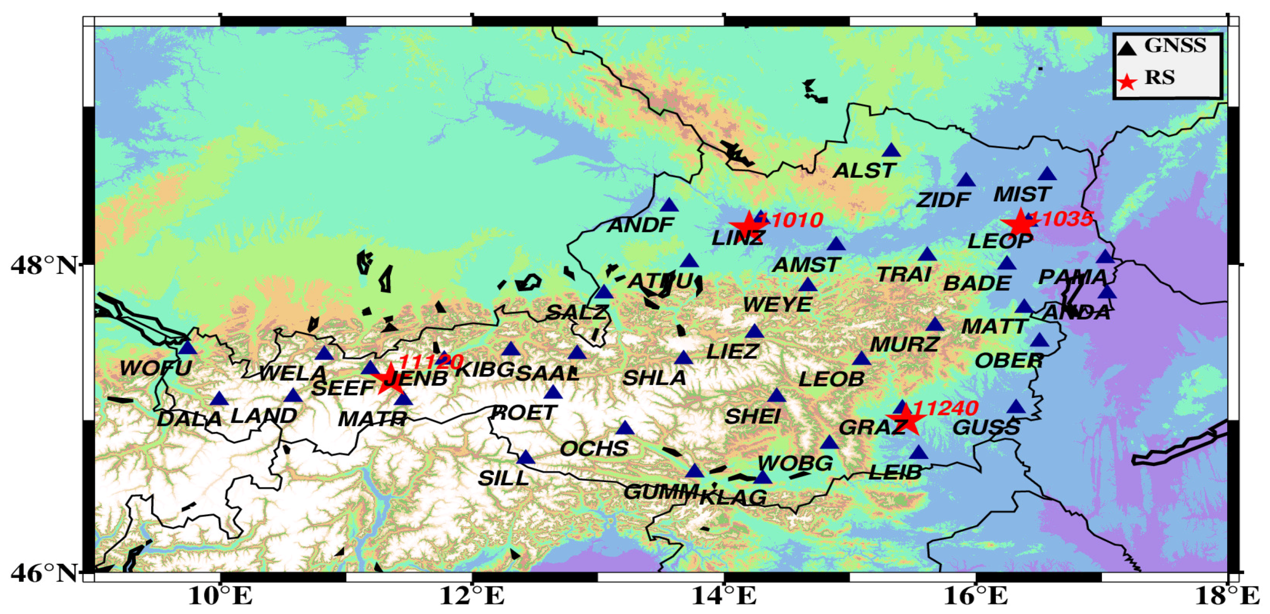
2. Data
2.1. GNSS ZTDs
2.2. Radiosonde Observations
2.3. Data Pre-Processing
3. Methodology
3.1. Tm Modelling
3.1.1. Empirical Models
- Bevis model
- GPT3 model
3.1.2. Developed Models
- Linear Model
- Polynomial Model
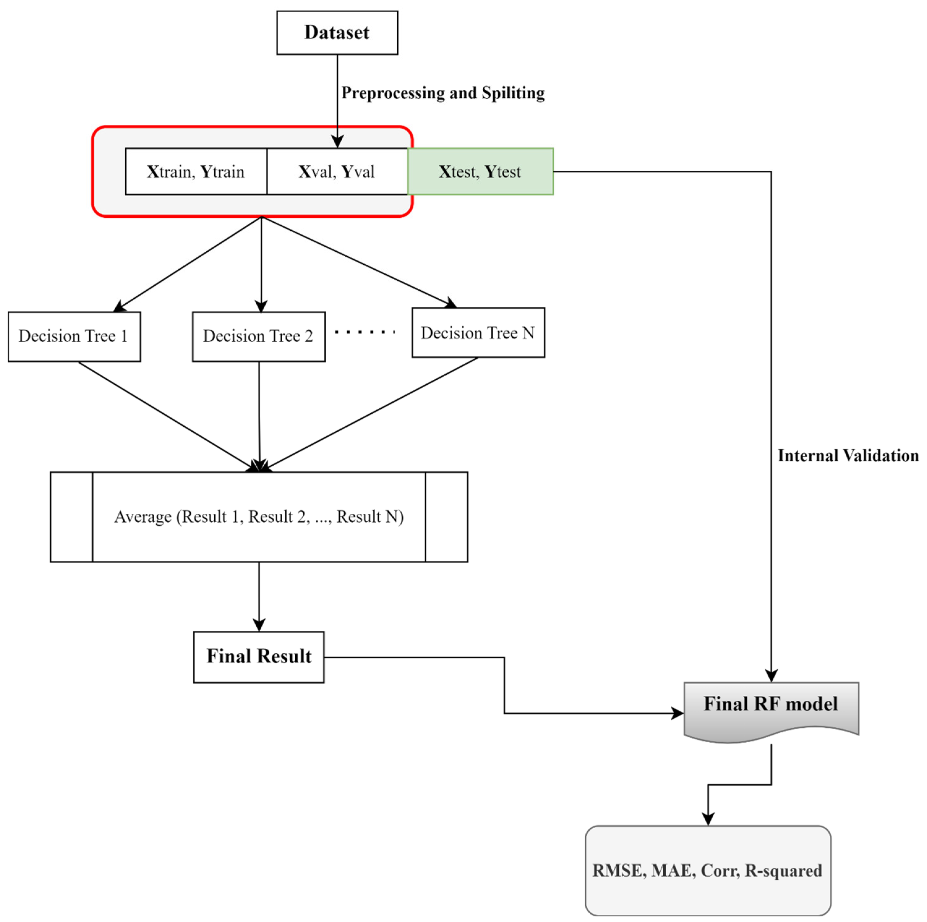
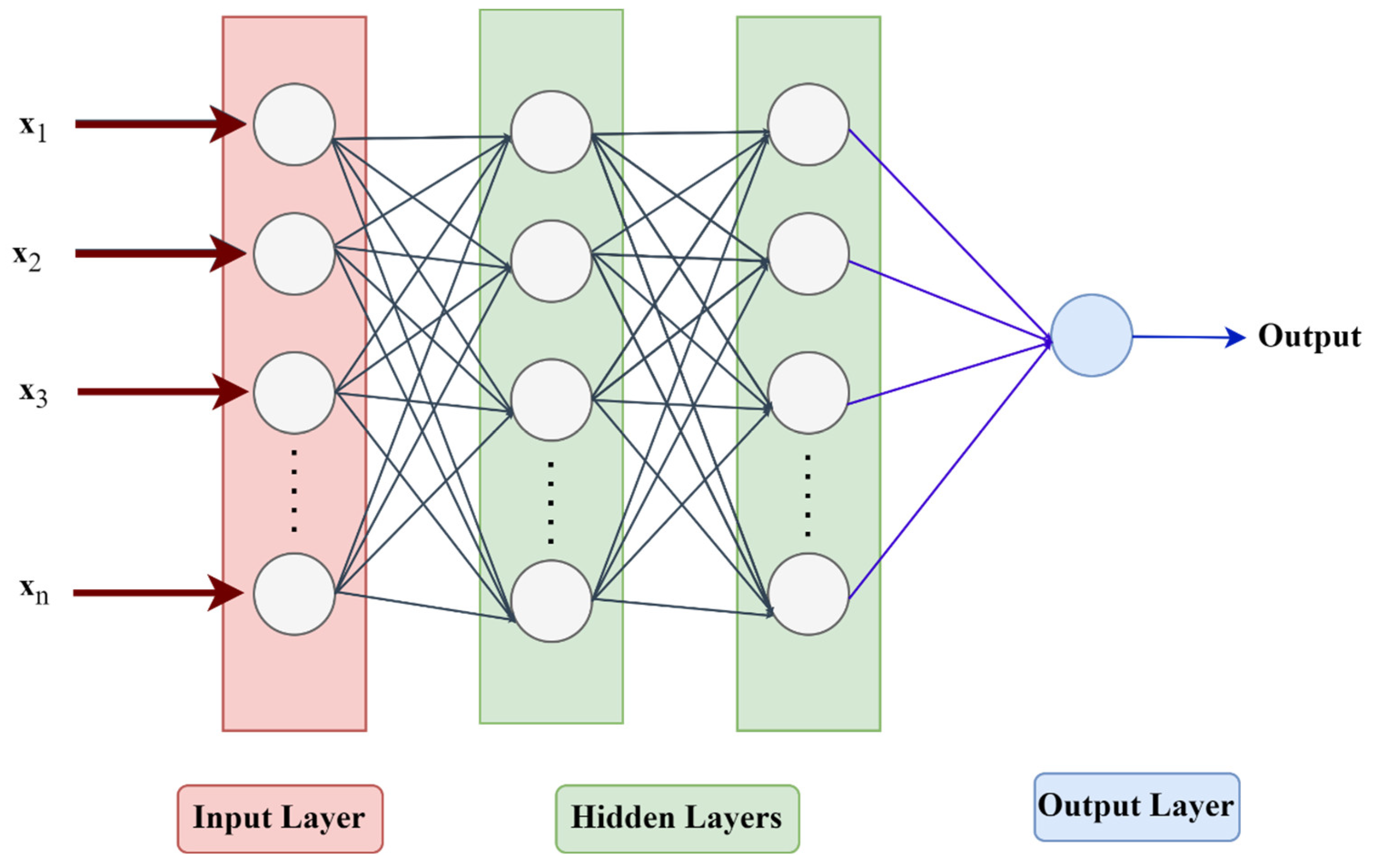
- Machine Learning Models (RF and ANN)
- -
- RF Method
- -
- ANN Method
3.2. PWV Modelling
3.2.1. Derived from GNSS Data
3.2.2. PWV Derived from Radiosonde Data
3.2.3. Developed Models
- -
- RF method
- -
- ANN method
3.3. Statistical Metrics
4. Numerical Results
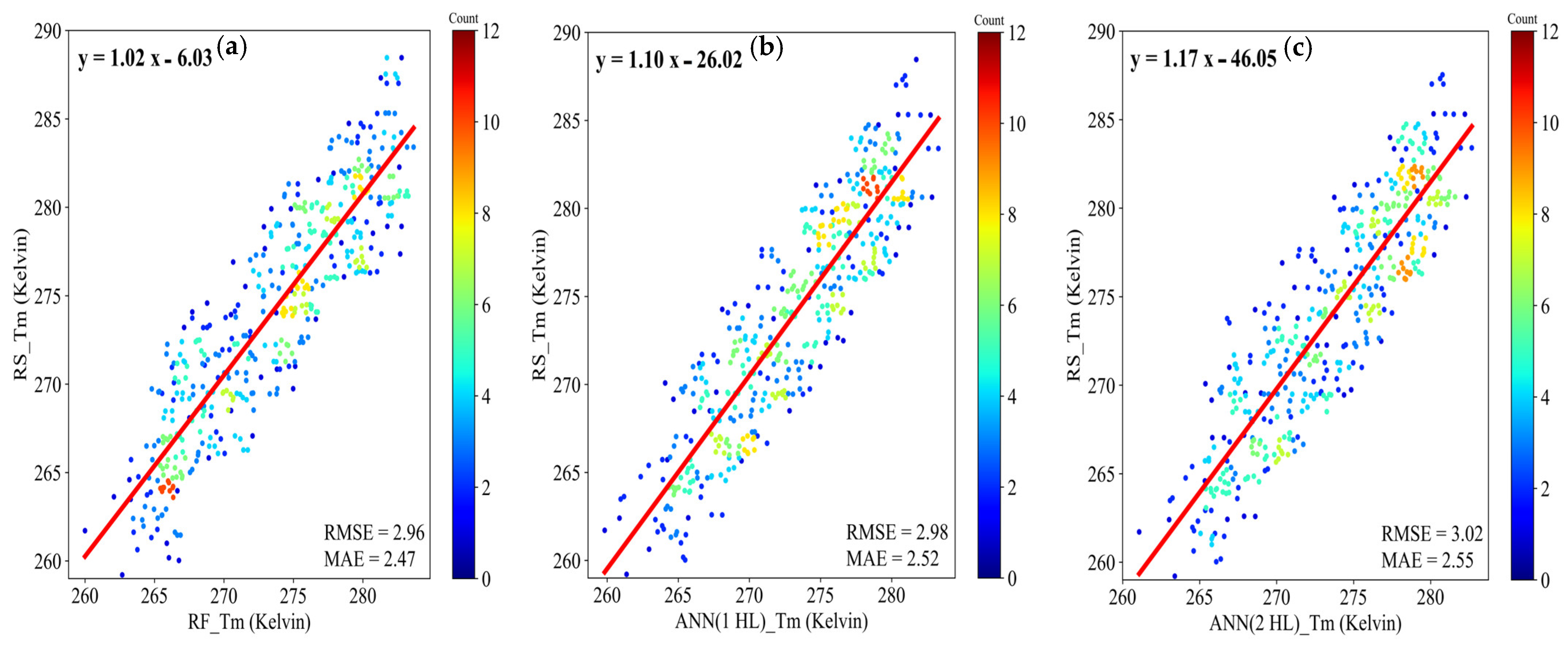
4.1. Accuracy Evaluation of
4.1.1. Internal Model Testing
4.1.2. External Model Testing
4.2. Accuracy Evaluation of
4.2.1. Internal Model Testing
4.2.2. External Model Testing
5. Conclusions
Author Contributions
Funding
Data Availability Statement
Acknowledgments
Conflicts of Interest
Appendix A

| Parameter | Value | Description |
|---|---|---|
| n_estimators | 1000 | The number of trees in the forest (100:100:1000) |
| max_features | sqrt | The number of features to consider when looking for the best split (‘sqrt’, ‘log2’) |
| max_depth | None | The maximum depth of the tree (None, (1:1:5)) |
| min_samples_leaf | 5 | The minimum number of samples required to be at a leaf node (1:1:5) |
| bootstrap | True | Whether bootstrap samples are used when building trees. If False, the whole dataset is used to build each tree [False, True] |
| Parameter | Description |
|---|---|
| Input layer | 1000 neurons, ‘selu’ activation function |
| Dropout layer | 0.0 dropout rate |
| Hidden layer | 1008 neurons, ‘selu’ activation function |
| Dropout layer | 0.0 dropout rate |
| Output layer | 1 neuron, ‘linear’ activation function |
| Optimizer | ‘rmsprop’ |
| Parameter | Description |
|---|---|
| Input layer | 1000 neurons, ‘selu’ activation function |
| Dropout layer | 0.0 dropout rate |
| First hidden layer | 1008 neurons, ‘sigmoid’ activation function |
| Dropout layer | 0.5 dropout rate |
| Second hidden layer | 1008 neurons, ‘sigmoid’ activation function |
| Dropout layer | 0.0 dropout rate |
| Output layer | 1 neuron, ‘linear’ activation function |
| Optimizer | ‘rmsprop’ |
Appendix B
| Parameter | Value | Description |
|---|---|---|
| max_features | sqrt | The number of trees in the forest (100:100:1000) |
| n_estimators | 800 | The number of features to consider when looking for the best split [‘sqrt’, ‘log2’] |
| max_depth | None | The maximum depth of the tree (None, (1:1:5)) |
| min_samples_leaf | 5 | The minimum number of samples required to be at a leaf node (1:1:5) |
| bootstrap | True | Whether bootstrap samples are used when building trees. If False, the whole dataset is used to build each tree [False, True] |
| Parameter | Value | Description |
|---|---|---|
| n_estimators | 900 | The number of trees in the forest (100:100:1000) |
| max_features | sqrt | The number of features to consider when looking for the best split [‘sqrt’, ‘log2’] |
| max_depth | None | The maximum depth of the tree (None, (1:1:5)) |
| min_samples_leaf | 5 | The minimum number of samples required to be at a leaf node (1:1:5) |
| bootstrap | True | Whether bootstrap samples are used when building trees. If False, the whole dataset is used to build each tree [False, True] |
| Parameter | Description |
|---|---|
| Input layer | 360 neurons, ‘sigmoid’ activation function |
| Dropout layer | 0.3 dropout rate |
| Hidden layer | 80 neurons, ‘sigmoid’ activation function |
| Dropout layer | 0.2 dropout rate |
| Output layer | 1 neuron, ‘linear’ activation function |
| Optimizer | ‘Adam’ |
| Parameter | Description |
|---|---|
| Input layer | 360 neurons, ‘sigmoid’ activation function |
| Dropout layer | 0.3 dropout rate |
| Hidden layer | 752 neurons, ‘sigmoid’ activation function |
| Dropout layer | 0.1 dropout rate |
| Output layer | 1 neuron, ‘linear’ activation function |
| Optimizer | ‘Adam’ |
| Parameter | Description |
|---|---|
| Input layer | 328 neurons, ‘sigmoid’ activation function |
| Dropout layer | 0.4 dropout rate |
| First hidden layer | 144 neurons, ‘sigmoid’ activation function |
| Dropout layer | 0.2 dropout rate |
| Second hidden layer | 848 neurons, ‘LeakyReLU’ activation function |
| Dropout layer | 0.1 dropout rate |
| Output layer | 1 neuron, ‘linear’ activation function |
| Optimizer | ‘Adam’ |
Appendix C
| Models | (mm) | (mm) | (%) |
|---|---|---|---|
| RF Scheme#1 | 1.95 | 2.48 | 95 |
| RF Scheme#2 | 2.11 | 2.66 | 95 |
| ANN 1 HL Scheme#1 | 1.96 | 2.50 | 96 |
| ANN 2 HL Scheme#1 | 2.02 | 2.57 | 96 |
| ANN 1 HL Scheme#2 | 2.04 | 2.56 | 96 |
| Models | (mm) | (mm) | (%) |
|---|---|---|---|
| RF Scheme#1 | 2.32 | 2.92 | 94 |
| RF Scheme#2 | 2.17 | 2.69 | 94 |
| ANN 1 HL Scheme#1 | 2.09 | 2.68 | 95 |
| ANN 2 HL Scheme#1 | 2.16 | 2.74 | 95 |
| ANN 1 HL Scheme#2 | 2.22 | 2.81 | 95 |
| Models | (mm) | (mm) | |
|---|---|---|---|
| RF Scheme#1 | 2.09 | 2.72 | 95 |
| RF Scheme#2 | 2.00 | 2.53 | 95 |
| ANN 1 HL Scheme#1 | 2.02 | 2.64 | 95 |
| ANN 2 HL Scheme#1 | 2.15 | 2.74 | 95 |
| ANN 1 HL Scheme#2 | 2.43 | 3.02 | 95 |
References
- Bevis, M.; Businger, S.; Herring, T.; Rocken, C.; Anthes, R.A.; Ware, R.H. GPS meteorology: Remote sensing of atmospheric water vapor using the global positioning system. J. Geophys. Res. Atmos. 1992, 97, 15787–15801. [Google Scholar] [CrossRef]
- Li, H.; Wang, X.; Wu, S.; Zhang, K.; Chen, X.; Qiu, C.; Zhang, S.; Zhang, J.; Xie, M.; Li, L. Development of an Improved Model for Prediction of Short-Term Heavy Precipitation Based on GNSS-Derived PWV. Remote Sens. 2020, 12, 4101. [Google Scholar] [CrossRef]
- Li, H.; Wang, X.; Choy, S.; Wu, S.; Jiang, C.; Zhang, J.; Qiu, C.; Li, L.; Zhang, K. A New Cumulative Anomaly-based Model for the Detection of Heavy Precipitation Using GNSS-derived Tropospheric Products. IEEE Trans. Geosci. Remote Sens. 2021, 60, 4105718. [Google Scholar] [CrossRef]
- Rocken, C.; Hove, T.V.; Johnson, J.; Solheim, F.; Ware, R.; Bevis, M.; Chiswell, S.; Businger, S. GPS/STORM: GPS sensing of atmospheric water vapor for meteorology. J. Atmos. Ocean. Technol. 1995, 12, 468–478. [Google Scholar] [CrossRef]
- Adavi, Z.; Rohm, W.; Weber, R. Analyzing Different Parameterization Methods in GNSS Tomography Using the COST Benchmark Dataset. IEEE J. Sel. Top. Appl. Earth Obs. Remote Sens. 2020, 13, 6155–6163. [Google Scholar] [CrossRef]
- Emardson, T.R.; Elgered, G.; Johansson, J.M. Three months of continuous monitoring of atmospheric water vapor with a network of global positioning system receivers. J. Geophys. Res. Atmos. 1998, 103, 1807–1820. [Google Scholar] [CrossRef]
- Huang, L.; Liu, L.; Chen, H.; Jiang, W. An improved atmospheric weighted mean temperature model and its impact on GNSS precipitable water vapor estimates for China. GPS Solut. 2019, 23, 51. [Google Scholar] [CrossRef]
- Liu, Z.; Zhang, T.; Li, J.; Xu, J.; Huang, L.; Zhou, L.; Liu, L. Analysis of Precipitable Water Vapor Change Based on GNSS Observations During Typhoon Mangkhut Event. In Proceedings of the China Satellite Navigation Conference (CSNC), Beijing, China, 22–25 May 2022. [Google Scholar]
- Rohm, W.; Yuan, Y.; Biadeglgne, B.; Zhang, K.; Le Marshall, J. Ground-based GNSS ZTD/IWV estimation system for numerical weather prediction in challenging weather conditions. Atmos. Res. 2014, 138, 414–426. [Google Scholar] [CrossRef]
- Zhao, Q.; Zhang, X.; Wu, K.; Liu, Y.; Li, Z.; Shi, Y. Comprehensive Precipitable Water Vapor Retrieval and Application Platform Based on Various Water Vapor Detection Techniques. Remote Sens. 2022, 14, 2507. [Google Scholar] [CrossRef]
- Dach, R.; Lutz, S.; Walser, P.; Fridez, P. Bernese GNSS Software, Version 5.2; User manual; Astronomical Institute, University of Bern: Bern, Switzerland, 2015. [Google Scholar]
- Saastamoinen, J. Contributions to the theory of atmospheric refraction. Part II: Refraction corrections in satellite geodesy. Bull. Géodésique 1973, 107, 13–34. [Google Scholar] [CrossRef]
- Vázquez, B.G.E.; Grejner-Brzezinska, D.A. GPS-PWV estimation and validation with radiosonde data and numerical weather prediction model in Antarctica. GPS Solut. 2013, 17, 29–39. [Google Scholar] [CrossRef]
- Jade, S.; Vijayan, M.S.M.; Gaur, V.K.; Prabhu, T.P.; Sahu, S.C. Estimates of precipitable water vapour from GPS data over the Indian subcontinent. J. Atmos. Sol. Terr. Phys. 2005, 67, 623–635. [Google Scholar] [CrossRef]
- Putri, N.S.E. Tropospheric Delay Models for GNSS in Indonesia; Technische Universität Wien: Vienna, Austria, 2021. [Google Scholar]
- Bevis, M.; Businger, S.; Chiswell, S.R.; Herring, T.A.; Anthes, R.A.; Rocken, C.; Ware, R. GPS meteorology: Mapping zenith wet delays onto precipitable water. J. Appl. Meteorol. Climatol. 1994, 33, 359–386. [Google Scholar] [CrossRef]
- Huang, L.; Wang, X.; Xiong, S.; Li, J.; Liu, L.; Mo, Z.; Fu, B.; He, H. High-precision GNSS PWV retrieval using dense GNSS sites and in-situ meteorological observations for the evaluation of MERRA-2 and ERA5 reanalysis products over China. Atmos. Res. 2022, 276, 106247. [Google Scholar] [CrossRef]
- Liang, H.; Cao, Y.; Wan, X.; Xu, Z.; Wang, H.; Hu, H. Meteorological applications of precipitable water vapor measurements retrieved by the national GNSS network of China. Geod. Geodyn. 2015, 6, 135–142. [Google Scholar] [CrossRef]
- Huang, L.; Mo, Z.; Xie, S. Spatiotemporal characteristics of GNSS-derived precipitable water vapor during heavy rainfall events in Guilin, China. Satell. Navig. 2021, 2, 13. [Google Scholar] [CrossRef]
- Guo, M.; Zhang, H.; Xia, P. Exploration and analysis of the factors influencing GNSS PWV for nowcasting applications. Adv. Space Res. 2021, 67, 3960–3978. [Google Scholar] [CrossRef]
- Sam Khaniani, A.; Motieyan, H.; Mohammadi, A. Rainfall forecast based on GPS PWV together with meteorological parameters using neural network models. J. Atmos. Sol.-Terr. Phys. 2021, 214, 105533. [Google Scholar] [CrossRef]
- Zhang, Z.; Lou, Y.; Zhang, W.; Liang, H.; Bai, J.; Song, W. Correlation Analysis between Precipitation and Precipitable Water Vapor over China Based on 1999–2015 Ground-Based GPS Observations. J. Appl. Meteorol. Climatol. 2022, 61, 1669–1683. [Google Scholar] [CrossRef]
- Ejigu, Y.G.; Teferle, F.N.; Klos, A.; Bogusz, J.; Hunegnaw, A. Tracking Hurricanes Using GPS Atmospheric Precipitable Water Vapor Field; Springer: Cham, Switzerland, 2020; Volume 152. [Google Scholar]
- Gong, Y.; Liu, Z.; Chan, P.K.; Hon, K.K. Assimilating GNSS PWV and radiosonde meteorological profiles to improve the PWV and rainfall forecasting performance from the Weather Research and Forecasting (WRF) model over the South China. Atmos. Res. 2023, 286, 106677. [Google Scholar] [CrossRef]
- Zhang, H.; Yuan, Y.; Li, W.; Zhang, B. A Real-Time Precipitable Water Vapor Monitoring System Using the National GNSS Network of China: Method and Preliminary Results. IEEE J. Sel. Top. Appl. Earth Obs. Remote Sens. 2019, 12, 1587–1598. [Google Scholar] [CrossRef]
- Sohn, D.-H.; Choi, B.-K.; Park, Y.; Kim, Y.C.; Ku, B. Precipitable Water Vapor Retrieval from Shipborne GNSS Observations on the Korean Research Vessel ISABU. Sensors 2020, 20, 4261. [Google Scholar] [CrossRef]
- Li, L.; Wang, X.; Wei, Y.; Wang, H. The New PWV Conversion Models Based on GNSS and Meteorological Elements in the China Region. Atmosphere 2022, 13, 1810. [Google Scholar] [CrossRef]
- Zhang, B.; Yao, Y. Precipitable water vapor fusion based on a generalized regression neural network. J. Geod. 2021, 95, 36. [Google Scholar] [CrossRef]
- Zheng, Y.; Lu, C.; Wu, Z.; Liao, J.; Zhang, Y.; Wang, Q. Machine Learning-Based Model for Real-Time GNSS Precipitable Water Vapor Sensing. Geophys. Res. Lett. 2022, 49, e2021GL096408. [Google Scholar] [CrossRef]
- Ma, Y.; Zhao, Q.; Wu, K.; Yao, W.; Liu, Y.; Li, Z.; Shi, Y. Comprehensive Analysis and Validation of the Atmospheric Weighted Mean Temperature Models in China. Remote Sens. 2022, 14, 3435. [Google Scholar] [CrossRef]
- Zhang, S.; Gong, L.; Gao, W.; Zeng, Q.; Xiao, F.; Liu, Z.; Lei, J. A weighted mean temperature model using principal component analysis for Greenland. GPS Solut. 2023, 27, 57. [Google Scholar] [CrossRef]
- Balidakis, K.; Nilsson, T.; Zus, F.; Glaser, S.; Heinkelmann, R.; Deng, Z.; Schuh, H. Estimating integrated water vapor trends from VLBI, GPS, and numerical weather models: Sensitivity to tropospheric parameterization. J. Geophys. Res. Atmos. 2018, 123, 6356–6372. [Google Scholar] [CrossRef]
- He, Q.; Shen, Z.; Wan, M.; Li, L. Precipitable Water Vapor Converted from GNSS-ZTD and ERA5 Datasets for the Monitoring of Tropical Cyclones. IEEE Access 2020, 8, 87275–87290. [Google Scholar] [CrossRef]
- Li, Q.; Yuan, L.; Chen, P.; Jiang, Z. Global grid-based Tm model with vertical adjustment for GNSS precipitable water retrieval. GPS Solut. 2020, 24, 73. [Google Scholar] [CrossRef]
- Manandhar, S.; Lee, Y.H.; Meng, Y.S.; Ong, J.T. A Simplified Model for the Retrieval of Precipitable Water Vapor from GPS Signal. IEEE Trans. Geosci. Remote Sens. 2017, 55, 6245–6253. [Google Scholar] [CrossRef]
- Wang, Z.; Zhou, X.; Liu, Y.; Zhou, D.; Zhang, H.; Sun, W. Precipitable water vapor characterization in the coastal regions of China based on ground-based GPS. Adv. Space Res. 2017, 60, 2368–2378. [Google Scholar] [CrossRef]
- Zhang, F.; Barriot, J.-P.; Xu, G.; Yeh, T.-K. Metrology Assessment of the Accuracy of Precipitable Water Vapor Estimates from GPS Data Acquisition in Tropical Areas: The Tahiti Case. Remote Sens. 2018, 10, 758. [Google Scholar] [CrossRef]
- Emardson, T.R.; Derks, H.J.P. On the relation between the wet delay and the integrated precipitable water vapour in the European atmosphere. Meteorol. Appl. 2000, 7, 61–68. [Google Scholar] [CrossRef]
- Mendes, V.B.; Prates, G.; Santos, L.; Langley, R.B. An Evaluation of the Accuracy of Models for the Determination of the Weighted Mean Temperature of the Atmosphere. In Proceedings of the ION 2000, National Technical Meeting, Anaheim, CA, USA, 26–28 January 2000; pp. 433–438. [Google Scholar]
- Suresh Raju, C.; Saha, K.; Thampi, B.V.; Parameswaran, K. Empirical model for mean temperature for Indian zone and estimation of precipitable water vapor from ground based GPS measurements. Ann. Geophys. 2007, 25, 1935–1948. [Google Scholar] [CrossRef]
- Wu, M.; Jin, S.; Li, Z.; Cao, Y.; Ping, F.; Tang, X. High-Precision GNSS PWV and Its Variation Characteristics in China Based on Individual Station Meteorological Data. Remote Sens. 2021, 13, 1296. [Google Scholar] [CrossRef]
- Long, F.; Hu, W.; Dong, Y.; Wang, J. Neural Network-Based Models for Estimating Weighted Mean Temperature in China and Adjacent Areas. Atmosphere 2021, 12, 169. [Google Scholar] [CrossRef]
- Böhm, J.; Heinkelmann, R.; Schuh, H. Short Note: A global model of pressure and temperature for geodetic applications. J. Geod. 2007, 81, 679–683. [Google Scholar] [CrossRef]
- Böhm, J.; Möller, G.; Schindelegger, M.; Pain, G.; Weber, R. Development of an improved empirical model for slant delays in the troposphere (GPT2w). GPS Solut. 2015, 19, 433–441. [Google Scholar] [CrossRef]
- Lagler, K.; Schindelegger, M.; Böhm, J.; Krásná, H.; Nilsson, T. GPT2: Empirical slant delay model for radio space geodetic techniques. Geophys. Res. Lett. 2013, 40, 1069–1073. [Google Scholar] [CrossRef]
- Yao, Y.; Zhang, B.; Xu, C.; Yan, F. Improved one/multi-parameter models that consider seasonal and geographic variations for estimating weighted mean temperature in ground-based GPS meteorology. J. Geod. 2014, 88, 273–282. [Google Scholar] [CrossRef]
- Yao, Y.B.; Zhang, B.; Yue, S.Q.; Xu, C.Q.; Peng, W.F. Global empirical model for mapping zenith wet delays onto precipitable water. J. Geod. 2013, 87, 439–448. [Google Scholar] [CrossRef]
- Sun, Z.; Zhang, B.; Yao, Y. A global model for estimating tropospheric delay and weighted mean temperature developed with atmospheric reanalysis data from 1979 to 2017. Remote Sens. 2019, 11, 1893. [Google Scholar] [CrossRef]
- Mateus, P.; Catalão, J.; Mendes, V.B.; Nico, G. An ERA5-Based Hourly Global Pressure and Temperature (HGPT) Model. Remote Sens. 2020, 12, 1098. [Google Scholar] [CrossRef]
- Yao, Y.; Zhu, S.; Yue, S.A. A globally applicable, season-specific model for estimating the weighted mean temperature of the atmosphere. J. Geod. 2012, 86, 1125–1135. [Google Scholar] [CrossRef]
- Wang, S.; Xu, T.; Nie, W.; Wang, J.; Xu, G. Establishment of atmospheric weighted mean temperature model in the polar regions. Adv. Space Res. 2020, 65, 518–528. [Google Scholar] [CrossRef]
- Zhao, Q.; Liu, K.; Zhang, T.; He, L.; Shen, Z.; Xiong, S.; Shi, Y.; Chen, L.; Liao, W. A Global Conversion Factor Model for Mapping Zenith Total Delay onto Precipitable Water. Remote Sens. 2022, 14, 1086. [Google Scholar] [CrossRef]
- Adavi, Z. Assessment of Various Processing Schemes and Solution Strategies to Improve the Performance of GNSS Tropospheric Tomography; Technische Universität Wien: Vienna, Austria, 2022. [Google Scholar]
- Li, L.; Zhang, K.; Wu, S.; Li, H.; Wang, X.; Hu, A.; Li, W.; Fu, E.; Zhang, M.; Shen, Z. An Improved Method for Rainfall Forecast Based on GNSS-PWV. Remote Sens. 2022, 14, 4280. [Google Scholar] [CrossRef]
- Sá, A. Tomographic Determination of the Spatial Distribution of Water Vapour Using GNSS Observations for Real-Time Applications; Wroclaw University of Environmental and Life Sciences: Wrocław, Poland, 2018. [Google Scholar]
- Sun, Z.; Zhang, B.; Yao, Y. Improving the Estimation of Weighted Mean Temperature in China Using Machine Learning Methods. Remote Sens. 2021, 13, 1016. [Google Scholar] [CrossRef]
- Vinutha, H.P.; Poornima, B.; Sager, B.M. Detection of Outliers Using Interquartile Range Technique from Intrusion Dataset. Adv. Intell. Syst. Comput. 2018, 701, 511–518. [Google Scholar] [CrossRef]
- Xie, W.; Huang, G.; Fu, W.; Shu, B.; Cui, B.; Li, M.; Yue, F. A quality control method based on improved IQR for estimating multi-GNSS real-time satellite clock offset. Measurement 2022, 201, 111695. [Google Scholar] [CrossRef]
- Yin, A.; Liu, H.; Yang, L.; Li, L. Analyzing the Impact of Climate Factors on GNSS-Derived Displacements by Combining the Extended Helmert Transformation and XGboost Machine Learning Algorithm. J. Sens. 2021, 2021, 9926442. [Google Scholar] [CrossRef]
- Davis, J.L.; Herring, T.A.; Shapiro, I.I.; Rogers, A.E.E.; Elgered, G. Geodesy by radio interferometry: Effects of atmospheric modeling errors on estimates of baseline length. Radio Sci. 1985, 20, 1593–1607. [Google Scholar] [CrossRef]
- Landskron, D. Modeling Tropospheric Delays for Space Geodetic Techniques; Technische Universität Wien: Vienna, Austria, 2017. [Google Scholar]
- Landskron, D.; Böhm, J. VMF3/GPT3: Refined discrete and empirical troposphere mapping functions. J. Geod. 2018, 92, 349–360. [Google Scholar] [CrossRef] [PubMed]
- Brown, S. Machine Learning, Explained; MIT Sloan School of Management: Cambridge, MA, USA, 2021. [Google Scholar]
- Lee, J.A.N. Computer Pioneer; IEEE Computer Society, History Committee: Piscataway, NJ, USA, 2021. [Google Scholar]
- Tajnai, C.E. Samuel Was Artificial Intelligence Pioneer. In Computing Research News; Computing Research Association: Washington, DC, USA, 1991. [Google Scholar]
- Kelleher, J.D.; Mac Namee, B.; D’Arcy, A. Fundamentals of Machine Learning for Predictive Data Analytics: Algorithms, Worked Examples, and Case Studies; The MIT Press: Cambridge, MA, USA, 2015. [Google Scholar]
- Shinde, P.P.; Shah, S. A Review of Machine Learning and Deep Learning Applications. In Proceedings of the Fourth International Conference on Computing Communication Control and Automation (ICCUBEA), Pune, India, 16–18 August 2018; pp. 1–6. [Google Scholar]
- Siemuri, A.; Kuusniemi, H.; Elmusrati, M.S.; Välisuo, P.; Shamsuzzoha, A. Machine Learning Utilization in GNSS—Use Cases, Challenges and Future Applications. In Proceedings of the International Conference on Localization and GNSS (ICL-GNSS), Tampere, Finland, 1–3 June 2021; pp. 1–6. [Google Scholar]
- Osman, A.I.A.; Ahmed, A.N.; Huang, Y.F.; Kumar, P.; Birmia, A.H.; Sherif, M.; Sefelnasr, A.; Ebraheemand, A.A.; El-Shafie, A. Past, Present and Perspective Methodology for Groundwater Modeling-Based Machine Learning Approaches. Arch. Computat. Methods Eng. 2022, 29, 3843–3859. [Google Scholar] [CrossRef]
- Ding, M. A neural network model for predicting weighted mean temperature. J. Geod. 2018, 92, 1187–1198. [Google Scholar] [CrossRef]
- Li, H.; Li, J.; Liu, L.; Huang, L.; Zhao, Q.; Zhou, L. Random Forest-Based Model for Estimating Weighted Mean Temperature in Mainland China. Atmosphere 2022, 13, 1368. [Google Scholar] [CrossRef]
- Breiman, L. Random Forests. Mach. Learn. 2001, 45, 5–32. [Google Scholar] [CrossRef]
- Lazri, M.; Soltane, A. Combination of support vector machine, artificial neural network and random forest for improving the classification of convective and stratiform rain using spectral features of SEVIRI data. Atmos. Res. 2018, 203, 118–129. [Google Scholar] [CrossRef]
- Łoś, M.; Smolak, K.; Guerova, G.; Rohm, W. GNSS-Based Machine Learning Storm Nowcasting. Remote Sens. 2020, 12, 2536. [Google Scholar] [CrossRef]
- Nakagawa, Y.; Miyauchi, T.; Higashino, T.; Okada, M. Application of random forest to classify weather observation into rainfall using GNSS receiver. In Proceedings of the IEEE VTS 17th Asia Pacific Wireless Communications Symposium (APWCS), Osaka, Japan, 30–31 August 2021; pp. 1–5. [Google Scholar]
- Ghassemi, B.; Dujakovic, A.; Żółtak, M.; Immitzer, M.; Atzberger, C.; Vuolo, F. Designing a European-Wide Crop Type Mapping Approach Based on Machine Learning Algorithms Using LUCAS Field Survey and Sentinel-2 Data. Remote Sens. 2022, 14, 541. [Google Scholar] [CrossRef]
- Liaw, A.; Wiener, M. Classification and Regression by randomForest. R News 2001, 2, 18–22. [Google Scholar]
- Liu, Y.; Wang, Y.; Zhang, J. New Machine Learning Algorithm: Random Forest. In Information Computing and Applications; ICICA, 2012; Lecture Notes in Computer Science; Liu, B., Ma, M., Chang, J., Eds.; Springer: Berlin/Heidelberg, Germany, 2012; Volume 7473. [Google Scholar]
- Pedregosa, F.; Varoquaux, G.; Gramfort, A.; Michel, V.; Thirion, B.; Grisel, O.; Blondel, M.; Prettenhofer, P.; Weiss, R.; Dubourg, V.; et al. Scikit-learn: Machine Learning in Python. J. Mach. Learn. Res. 2011, 12, 2825–2830. [Google Scholar]
- Brownlee, J. Data Preparation for Machine Learning: Data Cleaning, Feature Selection, and Data Transforms in Python. In Machine Learning Mastery; Jason Brownlee, 2020. [Google Scholar]
- Liashchynskyi, P.; Liashchynskyi, P. Grid Search, Random Search, Genetic Algorithm: A Big Comparison for NAS. arXiv 2019, arXiv:1912.06059. [Google Scholar]
- Rebala, G.; Ravi, A.; Churiwala, S. An Introduction to Machine Learning; Springer: Cham, Switzerland, 2019. [Google Scholar]
- Suparta, W.; Alhasa, K.M. Modeling of zenith path delay over Antarctica using an adaptive neuro fuzzy inference system technique. Expert Syst. Appl. 2015, 42, 1050–1064. [Google Scholar] [CrossRef]
- Benevides, P.; Catalao, J.; Nico, G. Neural Network Approach to Forecast Hourly Intense Rainfall Using GNSS Precipitable Water Vapor and Meteorological Sensors. Remote Sens. 2019, 11, 966. [Google Scholar] [CrossRef]
- Yuan, Q.; Shen, H.; Li, T.; Li, Z.; Li, S.; Jiang, Y.; Xu, H.; Tan, W.; Yang, Q.; Wang, J.; et al. Deep learning in environmental remote sensing: Achievements and challenges. Remote Sens. Environ. 2020, 241, 111716. [Google Scholar] [CrossRef]
- Selbesoglu, M.O. Prediction of tropospheric wet delay by an artificial neural network model based on meteorological and GNSS data. Eng. Sci. Technol. Int. J. 2020, 23, 967–972. [Google Scholar] [CrossRef]
- Gupta, A.; Nahar, P. Classification and yield prediction in smart agriculture system using IoT. J. Ambient. Intell. Humaniz. Comput. 2022, 14, 10235–10244. [Google Scholar] [CrossRef]
- Keras. BayesianOptimization Tuner. Available online: https://keras.io/api/keras_tuner/tuners/bayesian/ (accessed on 24 April 2023).
- Masum, M.; Shahriar, H.; Haddad, H.; Faruk, M.J.H.; Valero, M.; Khan, M.A.; Rahman, M.A.; Adnan, M.I.; Cuzzocrea, A.; Wu, F. Bayesian Hyperparameter Optimization for Deep Neural Network-Based Network Intrusion Detection. In Proceedings of the IEEE International Conference on Big Data (Big Data), Orlando, FL, USA, 15–18 December 2021; pp. 5413–5419. [Google Scholar]
- Nguyen, V. Bayesian Optimization for Accelerating Hyper-Parameter Tuning. In Proceedings of the IEEE Second International Conference on Artificial Intelligence and Knowledge Engineering (AIKE), Sardinia, Italy, 3–5 June 2019; pp. 302–305. [Google Scholar]
- Snoek, J.; Rippel, O.; Swersky, K.; Kiros, R.; Satish, N.; Sundaram, N.; Patwary, M.M.; Adams, R.P. Scalable Bayesian Optimization Using Deep Neural Networks. arXiv 2015. [Google Scholar] [CrossRef]
- Snoek, J.; Larochelle, H.; Adams, R.P. Practical Bayesian Optimization of Machine Learning Algorithms. arXiv 2012. [Google Scholar] [CrossRef]
- Victoria, A.H.; Maragatham, G. Automatic tuning of hyperparameters using Bayesian optimization. Evol. Syst. 2019, 12, 217–223. [Google Scholar] [CrossRef]
- Rüeger, J. Refractive index formulae for electronic distance measurements with radio and millimetre waves. UniServ Rep. 2002, 109, 758–766. [Google Scholar]
- Bolton, D. The Computation of Equivalent Potential Temperature. Mon. Weather. Rev. 1980, 108, 1046–1053. [Google Scholar] [CrossRef]
- Witt, L.D.; McKean, J.W.; Naranjo, J.D. Robust measures of associatiosn in the correlation model. Stat. Probab. Lett. 1994, 20, 295–306. [Google Scholar] [CrossRef]
- Osah, S.; Acheampong, A.A.; Fosu, C.; Dadzie, I. Deep learning model for predicting daily IGS zenith tropospheric delays in West Africa using TensorFlow and Keras. Adv. Space Res. 2021, 68, 1243–1262. [Google Scholar] [CrossRef]
- Ibrahim, K.; Huang, Y.F.; Ahmed, A.N.; Koo, C.H.; El-Shafie, A. A review of the hybrid artificial intelligence and optimization modelling of hydrological streamflow forecasting. Alex. Eng. J. 2022, 61, 279–303. [Google Scholar] [CrossRef]


| Dataset | Period | Spatial Resolution | Temporal Resolution | Usage |
|---|---|---|---|---|
| GNSS | Train: Jan 2018–Jun 2021 Test: Jul 2021–Jul 2022 | 39 Stations | 1 h | modelling |
| RS * | ): Jan 2010–Jun 2021 ): Jul 2021–Jul 2022 ): Aug 2022–April 2023 ): Aug 2022–April 2023 | 4 Stations | 3, 6, 12 h (see Table 2) | external validation |
| ERA5 | Jul 2021, April 2023 | 1 h | assimilation (External validation) |
| Station | Lat (deg) | Lon (deg) | H (metre) | Period | No. Launch 00:00 | No. Launch 06:00 | No. Launch 12:00 | No. Launch 18:00 |
|---|---|---|---|---|---|---|---|---|
| 11035 | 48.25 | 16.36 | 196 | Jan 2010–April 2023 | 5203 | 253 | 5203 | 139 |
| 11240 | 46.99 | 15.45 | 330 | Jan 2010–April 2023 | 6006 | 66 | 39 | 1 |
| 11120 | 47.26 | 11.35 | 579 | Jan 2010–April 2023 | 5816 | 111 | 65 | 40 |
| 11010 | 48.23 | 14.18 | 313 | August 2022–April 2023 | 450 | 4 | 2 | 0 |
| Model | Inputs | Scale | Trained Data |
|---|---|---|---|
| Bevis | Global/Regional | RS | |
| GPT3 | Global | ECMWF, VLBI |
| Model | Features |
|---|---|
| Linear | |
| Polynomial | |
| RF | |
| ANN |
| Parameters | Bernese Processing |
|---|---|
| Reference Frame | ITRF2014 |
| Satellite Orbit and Clock | IGS Final Products (CDDIS)/30 s |
| A priori Troposphere Model | Dry GMF |
| Gradient Model | CHENHER |
| Mapping Function | VMF1 |
| Ionospheric Model | Global Ionospheric Models ‘GIMs’ (CODE) |
| Ocean tidal loading | FES2004 model (Chalmers) |
| Ambiguity Fixing Strategy | Quasi Ionosphere-Free (QIF) |
| Cut-off angle | 5 degrees |
| Observation sampling rate | 30 s |
| Models | (K) | (K) | (%) | -Squared (%) |
|---|---|---|---|---|
| Polynomial | 2.82 | 3.46 | 84 | 70 |
| Linear | 3.14 | 3.85 | 80 | 62 |
| GPT3 | 3.58 | 4.46 | 79 | 50 |
| Bevis | 3.10 | 3.84 | 80 | 63 |
| RF | 2.38 | 2.97 | 89 | 79 |
| ANN (1 Hidden layer) | 2.45 | 3.02 | 88 | 77 |
| ANN (2 Hidden layer) | 2.46 | 3.04 | 88 | 77 |
| Models | (mm) | (mm) | (%) | -Squared (%) |
|---|---|---|---|---|
| RF Scheme#1 | 2.14 | 2.72 | 94 | 87 |
| RF Scheme#2 | 2.11 | 2.69 | 94 | 88 |
| ANN 1 HL Scheme#1 | 1.83 | 2.37 | 95 | 90 |
| ANN 2 HL Scheme#1 | 1.85 | 2.40 | 95 | 90 |
| ANN 1 HL Scheme#2 | 1.85 | 2.41 | 95 | 90 |
| Models | (mm) | (mm) | (%) |
|---|---|---|---|
| RF Scheme#1 | 2.17 | 2.78 | 94 |
| RF Scheme#2 | 2.14 | 2.68 | 94 |
| ANN 1 HL Scheme#1 | 2.05 | 2.64 | 95 |
| ANN 2 HL Scheme#1 | 2.13 | 2.71 | 95 |
| ANN 1 HL Scheme#2 | 2.13 | 2.70 | 95 |
Disclaimer/Publisher’s Note: The statements, opinions and data contained in all publications are solely those of the individual author(s) and contributor(s) and not of MDPI and/or the editor(s). MDPI and/or the editor(s) disclaim responsibility for any injury to people or property resulting from any ideas, methods, instructions or products referred to in the content. |
© 2023 by the authors. Licensee MDPI, Basel, Switzerland. This article is an open access article distributed under the terms and conditions of the Creative Commons Attribution (CC BY) license (https://creativecommons.org/licenses/by/4.0/).
Share and Cite
Adavi, Z.; Ghassemi, B.; Weber, R.; Hanna, N. Machine Learning-Based Estimation of Hourly GNSS Precipitable Water Vapour. Remote Sens. 2023, 15, 4551. https://doi.org/10.3390/rs15184551
Adavi Z, Ghassemi B, Weber R, Hanna N. Machine Learning-Based Estimation of Hourly GNSS Precipitable Water Vapour. Remote Sensing. 2023; 15(18):4551. https://doi.org/10.3390/rs15184551
Chicago/Turabian StyleAdavi, Zohreh, Babak Ghassemi, Robert Weber, and Natalia Hanna. 2023. "Machine Learning-Based Estimation of Hourly GNSS Precipitable Water Vapour" Remote Sensing 15, no. 18: 4551. https://doi.org/10.3390/rs15184551