Article

FSSBP: Fast Spatial–Spectral Back Projection Based on Pan-Sharpening Iterative Optimization

1
School of Geographical Sciences, Liaoning Normal University, Dalian 116029, China
2
National Marine Environmental Monitoring Center, Dalian 116023, China
3
School of Computer and Artificial Intelligence, Liaoning Normal University, Dalian 116029, China
*
Author to whom correspondence should be addressed.
Remote Sens. 2023, 15(18), 4543; https://doi.org/10.3390/rs15184543
Submission received: 25 June 2023 / Revised: 8 September 2023 / Accepted: 13 September 2023 / Published: 15 September 2023

Abstract

:
Pan-sharpening is an important means to improve the spatial resolution of multispectral (MS) images. Although a large number of pan-sharpening methods have been developed, improving the spatial resolution of MS while effectively maintaining its spectral information has not been well solved so far, and it has also been taken as a criterion to measure whether the sharpened product can meet the practical needs. The back-projection (BP) method iteratively injects spectral information backwards into the sharpened results in a post-processing manner, which can effectively improve the generally unsatisfied spectral consistency problem in pan-sharpening methods. Although BP has received some attention in recent years in pan-sharpening research, the existing related work is basically limited to the direct utilization of the BP process and lacks a more in-depth intrinsic integration with pan-sharpening. In this paper, we analyze the current problems of improving the spectral consistency based on BP in pan-sharpening, and the main innovative works carried out on this basis include the following: (1) We introduce the spatial consistency condition and propose the spatial–spectral BP (SSBP) method, which takes into account both spatial and spectral consistency conditions, to improve the spectral quality while effectively solving the problem of spatial distortion in the results. (2) The proposed SSBP method is analyzed theoretically, and the convergence condition of SSBP and a more relaxed convergence condition for a specific BP type, degradation transpose BP, are given and proved theoretically. (3) Fast computation of BP and SSBP is investigated, and non-iterative fast BP (FBP) and fast SSBP algorithms (FSSBP) methods are given in a closed-form solution with significant improvement in computational efficiency. Experimental comparisons with combinations formed by seven different BP-related post-processing methods and up to 18 typical base methods show that the proposed methods are generally applicable to the optimization of the spatial–spectral quality of various sharpening methods. The fast method improves the computational speed by at least 27.5 times compared to the iterative version while maintaining the evaluation metrics well.

Graphical Abstract

1. Introduction

The spectral features possessed by multi-band images enable the detection and discrimination of different materials in a scene, providing the possibility of fine-grained land observation and target identification. However, due to the limitation of the imaging mechanism, it is difficult to acquire satellite remote sensing images with both high spatial resolution and high spectral resolution directly through hardware devices [1,2]. Although multi-band images enhance the ability to express the corresponding feature attribute information, their geometric information acquisition capability is often limited or degraded [3]. Pan-sharpening, as an important means to enhance the spatial resolution of multi-band low-resolution (LR) multispectral images (MS) by software, which refers to the process of enhancing the spatial information and obtaining high-resolution (HR) MS images by using HR single-band panchromatic (PAN) images aligned with them [4]. Despite a long history of research, pan-sharpening is still one of the most challenging directions in remote sensing image processing [5], and many key issues still need to be further explored and solved. Among them, improving the spatial resolution of MS while effectively maintaining its spectral information has not been well solved so far, and it is also regarded as a criterion to measure whether the obtained high spatial resolution images can meet the practical needs [6]. To this end, the principle of spectral consistency to measure the spectral quality of the generated high spatial resolution images is proposed in the Wald protocol [7], which is widely used for image-sharpening quality assessment. That is, for any sharpened image, once it is degraded to the original LR scale, its spectral information should be as identical as possible to the original image.
In general, pan-sharpening methods can be divided into four categories [4,8,9,10]: component substitution (CS)-based methods, multi-resolution analysis (MRA)-based methods, optimization model (OM)-based methods (also often referred to as variational optimization or model-based methods) and deep learning (DL)-based methods. CS and MRA methods, also known as methods based on detail injection or second-generation techniques, are relatively lightweight, easy to implement and reproduce [11], and are mainstream accepted methods that are still attracting a lot of attention. In recent years, new generation methods represented by OM and DL have emerged and achieved good results in fields such as super-resolution reconstruction of natural images, and also have a great impact on remote sensing image pan-sharpening. Despite the larger potential, OM and DL methods are still generally suffering from complex parameter tuning, high computational overhead, and insufficient generalization capability [4,6], while experimental results and analyses from reviews [4,8,9,12,13] over the past few years show that the performance of fully optimized CS and MRA methods is not significantly weaker than that of many advanced OM or DL methods. This is probably due to the fact that the auxiliary HR PAN images provide relatively realistic and accurate spatial information a priori for the sharpening process, making the conventional methods also have a relatively high lower limit of quality, which is different from super-resolution. Considering the fundamental position of the traditional methods and their influence on the design of new generation methods, the development and optimization studies carried out for the second-generation methods are of great importance.
Among the major conventional methods, the MRA method is generally considered to have better spectral preservation ability than the CS method. This is because the low-frequency information of MS images embodying spectral components is retained more in the results, and better MRA methods usually imply proper modeling of the sensor spatial degradation process using filters. Nevertheless, it does not mean that MRA methods are well qualified for spectral consistency. For any non-ideal filter with a long trailing phenomenon, the frequency response intervals of its low-pass and high-pass portions overlap, which will lead to the spectral component of the result being inevitably affected by the PAN image, while its detail component will also be affected by the interpolated MS image. As an example, the generalized Laplacian pyramid (GLP) method [14], which uses a Gaussian filter adapted by a modulation transfer function (MTF), is superior to those filters that do not take into account the actual physical imaging process at all or only approximate it from the point of view of satisfying the consistency condition, such as box filters and Starck–Murtagh filters [15], etc. However, if the spatial degradation is further applied again to the output of the GLP, the result is not equivalent to the initial LR MS image [16], i.e., the spectral consistency condition is not satisfied.
In fact, ref. [17] reviewed the pan-sharpening methods from the perspective of Bayesian theory and pointed out that due to the lack of spectral consistency constraints in the equivalent maximum a posteriori probability model, typical methods including MRA and CS categories usually cannot effectively follow the spectral consistency principle. Two main solutions have been explored to improve this issue with the MRA approach.
The first approach is to combine the perfect reconstruction property of the multiscale transform with the consistency condition. It uses a downsampling process that includes, for example, a non-redundant discrete wavelet multiscale transform to achieve matching of LR-HR images at scale, enabling LR MS images to be directly presented in the results of multiscale decomposition. Since the generic wavelet low-pass filter based on critical sampling does not match the MTF curve reflecting the actual remote sensing imaging process, i.e., the blurring level of the images obtained by filtering with each of them is different, a custom construction of the filter is needed for the filter. This requires introducing MTF information into the wavelet low-pass filter design, and then completing the construction of the remaining filter bank based on some constraints (such as perfect reconstruction and aliasing suppression conditions). For example, ref. [16] considers the approximate coefficients of the transformed HR image to be solved as the LR MS image and at the same time considers its detail coefficients as wavelet detail coefficients of the PAN image. On this basis, the derivation of each filter coefficient is developed in combination with the corresponding constraints, and the resulting two-level decomposition is coupled by different filter banks. In [18], the initial results obtained by the GLP algorithm are decomposed with the discrete wavelet transform adapted by MTF, and then the LR MS image is replaced with its approximate components, keeping its original detail components unchanged. This approach increases the signal share of MS images in the results and thus reduces the difference between them, but due to the correlation of coefficients between different scales, it still does not guarantee that the results precisely satisfy the consistency condition, i.e., the approximate coefficients after decomposition again will not be the same as before reconstruction. This problem is not illustrated in [18], but it is reflected in the algorithmic idea of the subsequent literature [19].
The second way to improve the spectral inconsistency problem is similar to a further extension of [18], i.e., using the MS image as the initial approximate component and further iterating the approximate component substitution process in order to gradually reduce the error until finally approaching to reach the spectral consistency. In fact, this approach generally corresponds to the classic back-projection (BP) algorithm process in the super-resolution problem (see Section 2.1 for analysis).
There are several works that apply BP to the pan-sharpening problem. Among them, Vicinanza et al. [20] first used BP to improve the spectral consistency of various typical sharpening algorithms. The method recursively estimates the image that best fits specific constraints by applying a gradient descent-based BP procedure; Zhang et al. [17] focused on analyzing the spectral inconsistency generated by the sharpening method in principle, and then improved it with the help of BP. At the same time, the conjugate gradient method is used to speed up the iterative process. Both Liu et al. [21] and Jiao et al. [22] combined the high-pass modulation (HPM) algorithm with BP. The main difference between the two is the way in which the initial solution is enhanced. The former “Enhanced BP” (EBP) is to replace the MS image in the HPM algorithm with the sharpened results generated by other algorithms, and then modulate to obtain an enhanced initial solution. The latter mainly utilizes the FE-HPM [23], which includes a semi-blind blur kernel estimation process. The sharpened solutions from the FE-HPM and the method to be enhanced are weighted and averaged as the initial solution for the BP iteration.
The iterative optimization framework represented by BP has the advantages of strong versatility and easy implementation. However, the existing related work basically only stays at the level of direct use of the BP process, and lacks a more in-depth combination with the sharpening problem (see Section 2.2 for the analysis of related problems).
In this paper, we focus on the problems of improving spectral consistency based on BP in pan-sharpening, and extend and deepen the BP method from multiple dimensions to better serve the sharpening task, including three main works as follows.
(1) A spatial consistency condition corresponding to the spectral consistency condition is proposed. On this basis, a BP method that takes into account both spatial consistency and spectral consistency conditions is proposed, which is called “spatial–spectral BP” (SSBP) in this paper. The method introduces spectral degradation constraints based on the assumption of local linear combination on the basis of BP, which can effectively solve the spatial distortion problem of inaccurate detail injection in the sharpening initial solution while improving spectral consistency. The proposed method can better balance the spectral and spatial information to achieve high-quality sharpening results.
(2) The targeted discussion of BP convergence study in the sharpening field is supplemented. The proposed SSBP method is theoretically analyzed, and its convergence condition is given. A relaxed convergence condition is further given for a specific BP type—“degradation transpose BP” (see Section 2.1), which makes the proposed method more robust. The proposed convergence conditions are proved theoretically, and a practical verification analysis is also given. It is worth stating that the obtained conclusions are not limited to the field of sharpening, but are equally applicable to the application of spatial degradation terms (or so-called fidelity terms, data terms, etc.) in the form of degradation transposed BP in optimization problems.
(3) Research on the fast calculation methods of BP and SSBP obtain effective closed-form solutions for BP and SSBP by combining residual representation and ideal interpolation BP. This closed-form solution approach gives a non-iterative fast spatial–spectral BP algorithm, FSSBP. Compared with the corresponding iterative version, the computational efficiency of this algorithm is significantly improved while the evaluation indicators are similar, which makes it more valuable for engineering applications.

2. Related Works

2.1. Principle Analysis of BP-Based Spectral Consistency Improvement

Without loss of generality, the sharpened result performed by GLP is taken as an example to illustrate the principle of spectral consistency improvement based on BP. Denote the solution of the GLP algorithm as X 0 , and the interpolated MS and PAN are Y M ~ and Y P , respectively, then we have
X 0 = Y M ~ + g ( Y P Y P L )
where Y P L is the approximate component obtained by first extracting Y P and then interpolating
Y P L = Y P K d s s K u
where represents the convolution operation, K d is the Gaussian convolution kernel adapted according to the sensor MTF, and s a n d s represent downsampling and upsampling operations at resolution multiples s , respectively. The K u corresponding interpolation stage is often used for piecewise polynomial functions (such as the tap 23 filter [12]) that approximate ideal interpolation functions (such as the function s i n c ). Set representation of all variables as multi-band, for example g =   g k   , k = 1 , . . . , L , L is the number of bands in the MS image, and each band is calculated independently.
Taking X 0 as the initial solution, the result after the replacement of approximate components is X 1 , that is,
X 1 = Y M ~ + X 0 X 0 , L
among them, X 0 , L is the approximate component of X 0 , which corresponds to (2). From the relationship between (1) and (3), it can be seen that in addition to interpreting the two formulas as replacing their respective approximate components with Y M ~ , (3) can also be understood as replacing Y P with X 0 to perform the GLP algorithm ( g k is equivalent to 1 at this time), where X 0 is spectrally closer to Y M ~ than Y P .
Obviously, the output of (3) contributes to improvement but cannot directly satisfy the spectral consistency.
Further, denote the solution of the t -th iteration as X t ( t 1 ), and expand the convolution and sampling process in combination with (2), which can be described as
X t + 1 = X t + ( Y M X t K H s ) s K P
Equation (4) actually corresponds to the classic BP algorithm in the super-resolution problem [23], where the variable Y M is the original MS image at the LR scale. In the original BP algorithm, K H corresponds to the filtering operation that reflects the image spatial degradation process, which can correspond to Gaussian blur, motion blur and other degradation types. In the problem of remote sensing image sharpening, K H is K d , and K P is also called the projection filter, which corresponds to the inverse process of K H .
It should be noted that K P is not necessarily equal to K u in the BP algorithm. For the convenience of the following description, when K P is equal to K u , the BP is called “ideal interpolation BP” in this paper. It is more common to use the transpose of K H (that is, K H T , which is equivalent due to its symmetry) as K P . This is actually derived from the gradient calculation process (gradient descent solution) of the optimization problem corresponding to BP. For the convenience of distinguishing from the ideal interpolation BP, the BP in this case is called “degradation transpose BP” in this paper.
Furthermore, the initial solution is not limited to being provided by the GLP method. In fact, the result obtained by any sharpening method can be used as the initial solution. The purpose of the discussion above using GLP as a starting point is to clarify its relationship to BP (especially ideal interpolation BP). That is, the BP method can be regarded as an iterative version of the GLP method.

2.2. Analysis of Problems Based on BP Spectral Consistency Improvement

In terms of improving spectral consistency, the iterative optimization framework represented by BP has obvious advantages over the approach based on perfect reconstruction, and has also received more extensive attention and application. However, most of the current pan-sharpening methods involving BP simply treat it as post-processing, with insufficient consideration of the intrinsic characteristics and comprehensive optimization of pan-sharpening, and something that lacks in-depth research based at a theoretical level. This is reflected in the following aspects.
First, the observed PAN images that contain HR spatial information are not represented in the BP process. Although the BP process revolves around improving spectral consistency, spectral consistency is a necessary condition to meet the practical needs of pan-sharpening. With this constraint alone, it is difficult to guarantee high-quality results, effectively improving the spatial quality while maintaining its spectral consistency. In fact, in the process of pan-sharpening, the spectral properties of MS and the spatial properties of PAN, as dual properties that are both interrelated and mutually restrictive, jointly restrict the final sharpened result. A reasonable sharpening algorithm should take into account both aspects of information, and the improvement of spatial quality is also the original intention of the sharpening process. This makes it obvious that using only the original BP as an iterative optimization process is flawed from the perspective of generic sharpening quality improvement. It is conceivable that if only Y M ~ is used as the initial sharpening result for BP iterations (see Section 2.1), even if the spectral consistency condition is eventually nearly satisfied, the result may not contain a satisfactory spatial information enhancement component due to the lack of guidance from PAN information.
Second, there is a lack of research on convergence aspects related to the application of BP processes to the field of sharpening. In early studies on the convergence proof of BP [24,25], ref. [24] only proves the case when the resolution ratio is 1 (i.e., the deblurring problem), which is not suitable for sharpening or super-resolution applications. Ref. [25] expands [24] to an arbitrary ratio, which can theoretically be applied to the sharpening problem. However, there is no discussion on the validation of this convergence condition for specific sharpening conditions (e.g., for specific filter parameters). In addition, no further studies on BP convergence conditions have been seen in the context of sharpening applications, such as the existence of more relaxed convergence conditions in specific cases.
Third, there is a lack of fast computational research on BP. As an iterative processing algorithm, it is necessary to consider the efficiency improvement of BP despite its exponential level of convergence speed [25]. On the one hand, compared with the second-generation pan-sharpening method, which is known for its efficiency, the computational overhead added by BP iteration is significant. On the other hand, due to the high-dimensional characteristics of the data itself and the general use of high-precision and large-size convolution kernels, the problem of BP computation efficiency in remote sensing image sharpening is also more prominent compared to applications such as the super-resolution [3,13] of natural images. Given that its iterative computational process is similar or equivalent to that of gradient descent, the overall iterative convergence rate can be improved to some extent by using better iterative optimization algorithms such as the conjugate gradient method, but the improvement is limited.
To address the above problems, this paper investigates three aspects, namely, the spatial consistency condition, convergence and the acceleration strategy.

3. Methodology

3.1. Proposition of Spatial Consistency Conditions

In order to further improve the spatial quality of the BP iterative optimization framework, it is necessary to find spatially relevant constraints that can be associated with the PAN image to construct a “spatial BP”, and this requires first specifying the spatial consistency that can form a corresponding relationship with the spectral consistency. For the convenience of description, the original BP is referred to as “spectral BP” in this paper.
In the Wald protocol [7], in addition to the spectral consistency condition, two principles of vector compositionality and scalar compositionality are also specified, which can be combined and expressed as the compositional principle: the whole image (vector)/band image (scalar) of the sharpened image F should be as identical as possible to the whole image/band image of the ideal image G T . The G T here is ideally the imaging result that the MS sensor should obtain with the same spatial resolution as the PAN image. The principle of compositionality defined on the HR scale is theoretically a sufficient and necessary condition to meet the needs of sharpening applications. However, since G T is not actually accessible and the content does not additionally contain specific descriptions or assumptions about the relationship between the corresponding images except for the spatial resolution factor, this means that the principle is not a direct guide for the spatial constraints to be sought.
Since the answer cannot be obtained directly from the Wald protocol, it is necessary to further consider spatial consistency from other perspectives. Review the equivalent representation of spectral consistency: the spectral information of the resulting sharpened image F after spatial degradation should be consistent with the original MS image. If the characteristic of spatial–spectral duality is considered, the following expression (or hypothesis) can be given: the spatial information of the sharpened image F after spectral degradation should be consistent with the original PAN image. This paper defines this formulation as the principle of spatial consistency.
In fact, from the perspective of physical imaging of MS and PAN sensors, the above principle of spatial consistency is reasonable. Specifically, given that the mutually matched PAN image is in a broad–narrow-band relationship with the MS image, the PAN image can be effectively modeled as the result of superimposing the images of the bands in F , i.e., obtained by spectral degradation (or spectral transformation) of F when the spectral response intervals of the two overlap to a high degree. If the wavelength in the spectral dimension is analogous to the frequency in the spatial dimension, then the PAN image compared to the MS band image is similar to the relationship between the results of filtering the same image by an all-pass filter and several band-pass filters in different frequency ranges.
It is worth mentioning that, like the correlation between spectral BP and MRA-based GLP (see Section 2.1), the proposed spatial BP also has a similar correlation with CS-based Gram–Schmidt Adaptive (GSA) [26]. That is, the spatial similarity is constrained by a linear combination of bands in GSA. However, no previous work has considered its iterative form and combined it with BP, and no work has pointed out the above-mentioned association.

3.2. Proposition of Spatial–Spectral Back-Projection Iterative Model (SSBP)

Considering that the spectral degradation is not usually depicted in the convolution form, for the convenience of presentation, the latter equations are written in the matrix–vector form, where the transformation or convolution process is expressed in matrix form and the variables are expressed in column-vector form. The relevant variable symbols are described in Table 1.
According to this variable symbology, the spectral consistency condition is equivalent to the following spatial degradation model:
y M = M G x
where x represents any HR-sharpened image vector that satisfies the spectral consistency condition. Obviously, if x does not satisfy the spectral consistency condition, a non-zero spectral error term e λ = y M M G x will be generated. The spectral BP process is the process of gradually reducing the e λ . Its iteration can be written as
x k + 1 = x k + W G e k λ
where e k λ = y M M G x k is the spectral error term for k iterations.
Equation (6) is equivalent to (4). According to (5) and (6), and the spatial–spectral duality relationship, the spectral degradation model based on the spatial consistency condition can be established accordingly:
y P = M R x
and the iterative form of spatial BP is
x k + 1 = x k + W R e k s
where the spectral degradation matrix M R is usually calculated by the multiple linear regression between the PAN and MS images at the LR scale, as described previously, and e k s = y P M R x k is the spatial error term for k iterations.
Similar to spectral BP, there are also two ways to take M R in (8). One is to directly make W R = M R T , that is, the spatial degradation transpose BP. The other type can be consistent with the setting of the inverse spectral transform (gain vector) in the Gram–Schmidt or GSA method, where the corresponding coefficients are derived from the Gram–Schmidt orthogonalization process [12]. Combining (6) and (8), the following SSBP expression can be obtained:
x k + 1 = x k + τ λ W G e k λ + τ s W R e k s
where τ λ and τ s are the weights corresponding to the above error terms, respectively.

3.3. Model Convergence Analysis

3.3.1. Convergence Conditions for Spatial–Spectral BP

Review the BP convergence condition given in [25]:
C B P = K δ K P K H s   1 < 1
where K δ represents the unit impulse response centered at the (0,0) point. Since this formula is defined based on convolution, it is not applicable to spatial BP and SSBP cases that include linear spectral transformation operations (non-convolution). Therefore, it is necessary to study the convergence based on matrix representation.
First, the relevant variables are formed into a combined representation. Let y = y M y P , e k = e k λ e k s , τ = τ λ τ s T , M = M G M R , and W = W G W R , where τ λ and τ s are the vector versions of τ λ and τ s , respectively, that is, τ λ = τ λ 1 and τ s = τ s 1 . Vector 1 is an all-ones vector with the same dimension as
. With the above representation, (5) and (7) can be combined into the following degradation model:
y = M x
Furthermore, (9) can be further organized as y
x k + 1 = x k + τ W e k
Theorem 1. 
When the norm of any matrix corresponding to  I τ M W  is less than 1, (12) converges.
Proof. 
Since (11) and (12) are formally consistent with the spectral BP correlation equations, respectively, inspired by the proof idea in [25], an expansion of e k in (12) yields
e k = y M x k = y M x k 1 + τ W e k 1 = ( y M x k 1 ) τ M W e k 1 = e k 1 τ M W e k 1 = ( I τ M W ) e k 1
where I is the unit matrix with appropriate dimension, which actually corresponds to K δ in (10).
Further, by the subproductivity between any vector norm and its compatible matrix norm [27], it follows that
I τ M W e k 1 ( I τ M W ) e k 1
From (13) and (14), we have
e k = I τ M W e k 1 I τ M W e k 1 I τ M W 2 e k 2 ( I τ M W ) k e 0
That is 0 e k ( I τ M W ) k e 0 .
When I τ M W < 1 , there is l i m k ( I τ M W ) k e 0 = 0 .
Thus, we have l i m k e k = 0 , i.e., the SSBP converges. ☐
According to the above theorem, the convergence condition of SSBP is
I τ M W < 1
Since both spectral BP and spatial BP are special cases of SSBP (the corresponding weights are set to 0), their convergence conditions can also be generalized by (15).

3.3.2. Relaxed Convergence Condition for Degradation Transpose Back Projection

The previous section gave the convergence condition for SSBP including spectral BP, which also holds true for degradation transpose BP (see Section 2.1). However, whether it is based on the convolutional Formula (10) or the matrix-based Formula (15), it can be seen from Section 3.4 below that they may have certain problems or uncertainties due to factors such as sampling offset position and image size during actual inspection. To this end, this section gives more relaxed convergence conditions for the degradation transpose spectral BP. Before that, another condition for spectral BP convergence is given first.
For the convenience of discussion, the spectral error term e k λ in (6) is expanded and the symbol is simplified:
x k + 1 = x k + W G e k λ = x k + y M ~ G x k
where G = W G M G , y M ~ = W G y M .
To prove the convergence of (16), in addition to proving that e k λ decreases with iteration, we can also prove that x k is equal to x k 1 when k approaches infinity. This is further organized by
x k x k 1 = x k 1 G x k 1 x k 2 + G x k 2 = I G x k 1 x k 2 = I G k 1 ( y M ~ G x 0 )
where x 1 x 0 = y M ~ G x 0 .
Further let A = I G , from (17), when A k 1 y M ~ G x 0 = 0, it means that the convergence is achieved. Since A in this formula is similar in form to the corresponding term in (13), it is natural to think that the convergence condition should also be A < 1 . However, this is not the case. Since the iteration of x k can also be written as x k = A x k 1 + y M ~ , it is further expanded as
x k = A x k 1 + y M ~ = A A x k 2 + y M ~ + y M ~ = A 2 x k 2 + A y M ~ + y M ~ = A k 1 x 1 + j = 1 k 2 A j y M ~ + y M ~ = A k x 0 + j = 0 k 1 A j y M ~
For (18), if A < 1 ,then there is l i m k A k x 0 = 0 . This means that the final result of BP iterative convergence is independent of the initial solution x 0 , but obviously this does not match the facts, which shows that this assumption does not hold for a reasonably efficient BP iterative process.
In fact, for A that matches the actual situation, there is ρ A = 1 , where ρ A is the spectral radius of A . According to the nature of spectral radius, there is λ ρ A A , where λ is an arbitrary eigenvalue of λ . An important application of the spectral radius is to provide the largest lower bound for the norm of a matrix.
Based on the above analysis, the following corollary is given:
Corollary 1. 
When  ρ A = 1 , we have  l i m k ( x   k x k 1 ) =  0.
Proof. 
When ρ A = 1 , it means A is semi-convergent, that is, l i m k A k exists, and there is
l i m k A k = I ( I A ) ( I A ) D
where ( · ) D is the Drazin inverse [26]. To further organize it, the following hold:
l i m k A k = I ( I I + G ) ( I I + G ) D = I G G D
l i m k ( x k x k 1 ) = ( I G G D ) ( y M ~ G x 0 ) = y M ~ G G D y M ~ G x 0 + G G D G x 0
Since the Drazin inverse is a kind of generalized inverse, for any matrix M , there is M M D M = M . Therefore, (21) can be further written as
y M ~ G G D y M ~ G x 0 + G x 0 = ( I G G D ) y M ~
As the l i m k A k corresponding to I G G D semi-converges to a non-zero matrix, and y M ~ is modeled as the result of further interpolation after the spatial degradation of the HR image to be calculated, this transformation process just corresponds to G (see (5)). That is, y M ~ = G x , where x corresponds to any HR image that meets the spectral consistency condition. Substituting into (22) can further obtain
( I G G D ) y M ~ = I G G D G x = G x G G D G x = G x G x = 0
Therefore, Corollary 1 holds. ☐
In this paper, the convergence condition based on the LR scale error term in (10) and (15) is called the “LR scale condition”, and the convergence condition corresponding to Corollary 1 is called the “HR scale condition”. The correlation between the two can be obtained as follows (based on the degradation transpose BP):
I M G T M G M G T = M G T I M G M G T
It can be found that the I M G T M G on the left side of (24) is after the interpolation operation of M G T , and the operation of I M G M G T on the right side of the equation is before the interpolation, that is, the two operations correspond to the HR scale and the LR scale respectively.
After Corollary 1 is drawn, a further conclusion about the degradation transpose BP is given:
Corollary 2. 
For degradation transpose BP with Gaussian low-pass filter kernel, it must be the case that  ρ A = 1 .
Proof. 
In degradation transpose BP, since the data matrix G = M G T M G is a real symmetric matrix (or Hermitian matrix) and singular at the same time, it is known that G is positive semi-definite [28], and all its eigenvalues are non-negative. Combining with A = I G , it follows that ρ A = 1 is satisfied when ρ ( G ) 2 is satisfied, at which point ρ A can all be determined by the minimum eigenvalue (i.e., 0 value) of G . Therefore, the proof of Corollary 2 only needs to verify that the condition ρ ( G ) 2 is satisfied.
In fact, when K H is a Gaussian low-pass filter kernel, according to the requirement of low-pass filter energy preservation and the definition of Gaussian function, it can be known that its coefficients have the characteristics of normalization (sum is 1) and non-negativity, because each column of H is composed of cyclic translation of coefficients in K H , such that the maximum column sum matrix norm (i.e., l 1 norm) of H is 1 based on the above characteristics of K H coefficients, i.e., H 1 = 1 .
Further, from the properties of M G = S H and the downsampling matrix S , it can be seen that the elements in M G are actually the result of r 2 times downsampling on H by row, where r is the resolution ratio, which means that M G 1 < 1 , and its corresponding Gaussian function peak is retained after the S sampling operation. At the same time, since H is a symmetric matrix and the S process does not change its column elements, there is M G T 1 = 1 . Combined with the above analysis, using the subproductivity of the matrix norm, we can obtain
G 1 = M G T M G 1 M G T 1 M G 1 < 1
Since the spectral radius is the lower bound of the matrix norm, it is easy to obtain ρ ( G ) < 1 from (25), and Corollary 2 holds. ☐
From the above proof process, it can be found that for degradation transpose BP, the convergence condition mainly depends on S and H , which are determined by r and K H , respectively. When K H is a Gaussian blur kernel, the larger r is, the smaller ρ ( G ) is. At this point, Corollary 2 holds for sharpening, super-resolution ( r 2 ) and deblurring applications (i.e., r = 1 , S = I ). However, when K H is another filter type or the BP type is ideal interpolation, additional discussion must be made according to the specific coefficients of the matrix. For example, for the bicubic filter (i.e., tap-7) that is often used in the degradation/interpolation process in natural image super-resolution applications, the l 1 norm is greater than 1 due to the existence of negative values in the sidelobe coefficients; for an ideal interpolator, for the purpose of energy preservation, the coefficient sum of the corresponding filter is usually r 2 times that of the degradation stage; so, the corresponding qualitative conclusions cannot be drawn simply through the above analysis process. But for sharpening applications where K H is fixed as a Gaussian blur kernel, Corollary 2 is always satisfied. Combining Corollary 1 and Corollary 2, it can be seen that the degradation transpose BP within the scope of this paper must converge.
A question to ponder is whether Corollary 2 is equally valid if the LR scale condition is used. In fact, the relationship between the matrix spectral radius and the norm shows that when the LR scale condition is satisfied, there should be ρ ( I M G M G T ) < 1 . Note that this condition is stricter than the original norm-based condition because a spectral radius less than 1 does not mean that any norm is less than 1, but the opposite holds. This means that the eigenvalue range of M G M G T , which is also a real symmetric array, should be within (0, 2). Based on the previous analysis of (25), it is easy to conclude that ρ ( M G M G T ) is also less than 1. The key then lies in discerning whether all the eigenvalues of M G M G T are greater than 0, i.e., whether M G M G T is a positive definite matrix. Although the feasibility of this idea is not excluded, the advantage of using the HR scale condition is that the process of determining the lower bound of the relevant matrix eigenvalues is simpler and more straightforward, and it additionally includes the cases where the eigenvalues can be 0 and 2. Nevertheless, it should be noted that the LR scale condition involves a much smaller data size than the HR scale condition, implying that the LR scale condition should be a more convenient choice when verifying the convergence of the conventional BP.

3.4. Application Analysis of Model Convergence Condition

The convergence conditions in Section 3.3.1 and Section 3.3.2 above involve two types of representations, convolution and matrix, respectively, and both representations have their own advantages and disadvantages in practical applications.
On the one hand, the advantage of convolution-based representation is that the calculation process is independent of the actual image size, and only the convolution operation needs to be completed according to the filter size; so, the computational overhead of the verification process is very low. However, the convergence condition (10) and its proof process given in [25] do not specify some details of the sampling method. In practical applications, it is affected by the finite impulse response (FIR) filter size, scaling ratio and sampling offset position. The effect of the setting will likely result in undefined or unsatisfied conditions. In (10), the non-zero element in the unit pulse K δ corresponds to the center position of the filter K S = K P K H s , and the size of the two is the same. However, there may be odd and even size results at different sampling positions, corresponding to the schematic diagrams of (a) and (b) in Figure 1, where the blue and white grids denote the samples that are retained and discarded after sampling, respectively.
Filters with symmetry about the central spike are usually of odd size (e.g., K H ). For ideal interpolators in sharpening (e.g., the most common tap-23), a separable, two-step interpolation implementation is generally used. Although the number of coefficients of the two-fold one-dimensional convolution kernel is odd, its equivalent two-dimensional filter for direct four-fold interpolation is of even size, implying that the common K P should be of even size. In contrast, even-size filters of two-fold ratio (e.g., tap-8), although less common in other applications, have been considered in pan-sharpening [29], corresponding to the odd-size K P . For the common case where K P and K H are of even and odd sizes, respectively, the size of the result obtained by the two convolution operations is an even number (the sum of the two minus 1), and the single peak exists but the position is not centered. Whether symmetrical results can be obtained in this case with respect to the central single spike depends on the sampling offset position. If both the K P and K H convolution kernels are of odd size, then the result is still odd. If the conventional 4-fold downsampling is further applied to it, the resulting K S must not be divisible, and the parity of its size and the retained samples will also be determined by the sampling position. If the K S generated by any combination of the above is an even size, it means that the center position is between adjacent pixel grid points, and the operation with K δ will not be accurately defined. In this case, if the position of the adjacent pixel is regarded as the center, there may be a contradictory situation where the convergence condition is not satisfied but still converges in practice. Ref. [30] pointed out that the sampling position should start from the central part of the convolution kernel.
On the other hand, the matrix representation of the convergence condition has the advantage that it can include non-convolutional operations, such as the spatial consistency condition related operations in this paper (see Section 3.1). At the same time, since the sampling operation under the matrix representation is aimed at the image matrix, and its dimension matches the image size, there are no uncertainties caused by the non-divisible size and the above-mentioned sampling position. However, the correlation with image size also brings the problem of large computational overhead. For example, even for a small image of 56 × 56 pixels in size, the corresponding process matrix will have a maximum dimension of 3136 × 9216 with the introduction of boundary processing, meaning that it cannot be tested directly at the actual image dimensions. However, the matrix product operation corresponding to the relevant convolution operation can be accelerated and reduced in storage overhead through Fourier transform.
Figure 2 illustrates the validation of the BP convergence condition for the sharpening problem with a resolution ratio of 4, where (a) illustrates the content of the matrix G (the image is cropped for viewing due to the repetition of the style), and (b) shows the validation of different K P and K H (corresponding to different MTF Nyquist frequencies) in (10). When K P is “MTF”, it corresponds to the transpose of the degradation operation, and “general” corresponds to the interpolation method commonly used in Hyperspectral sharpening (supporting non-even magnification) [31]. Note that the method in this paper is also applicable to the Hyperspectral sharpening problem. “tap-7” corresponds to bicubic interpolation. The “tap-8” is not shown due to the above sampling offset uncertainty, and is verified to be converged by the actual sharpening process. The MTF Nyquist frequency of different MS sensors is typically around 0.2–0.4, which is covered by the range tested (horizontal axis). It can be seen from the numerical value of the vertical axis in the figure that the tested conditions all satisfy the convergence ( C B P is less than 1).

3.5. Fast Computation of Models

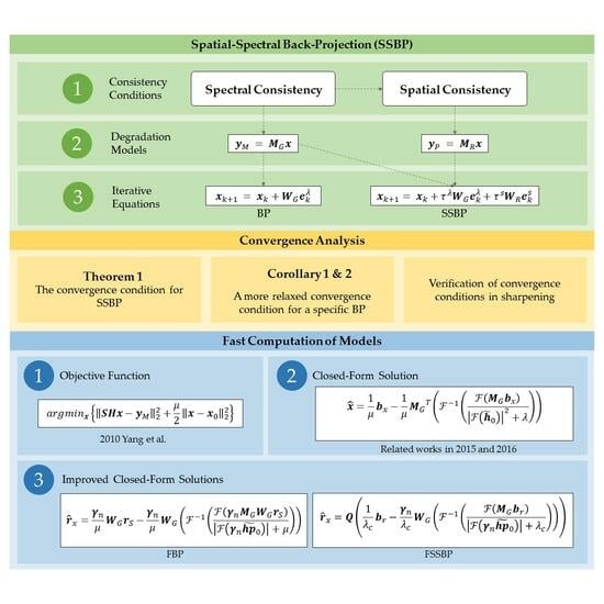
This section further develops the discussion on the acceleration of BP and SSBP algorithms, and two available routes for exploration are considered.
One way of thinking is to continue the derivation of (18) based on mathematical induction, and discuss the asymptotic solution when k approaches infinity, which is
lim k ( A k x 0 + j = 0 k 1 A j y M ~ )
However, the computational procedure of this problem is not clear. First, although the first term in (26) yields a theoretically convergent solution based on the Drazin inverse, no efficient and feasible algorithm for finding the Drazin inverse has been found to exist. Secondly, the second term of the equation generates undesirable computational procedures when finding the partial sum of the matrix isometric series, i.e., it involves singular matrix inversion, leading to unreachable results. Finally, given that the dimensionality of A is too high to explicitly declare it in the program, even if a theoretical solution can be obtained, it cannot be effectively applied to practical problems.
Therefore, this paper considers another idea: to associate the BP algorithm with the optimization problem. This means finding its equivalent or approximate objective function and exploring possible closed-form solutions for that objective function.

3.5.1. Fast BP

According to the relationship between BP and spectral consistency, the following ordinary least squares problem can be obtained from the spatial degradation process:
a r g m i n x { M G x y M 2 2 }
The M G x y M 2 2 term is often referred to as the data fidelity term, and the relationship between the gradient degradation of this formula and the BP algorithm can be established by setting the implicit initial solution conditions (set the iterative initial solution to be x 0 ), that is, the degradation transposition BP. However, due to the ill-posedness of the problem and the lack of regularization in the objective function, it is impossible to obtain numerically stable closed-form solutions only by relying on the data fidelity term (i.e., the globally optimal least-squares solution, which involves inverting the data matrix entries). Even if a regular term about x itself (e.g., Tikhonov, total variational regularization, etc.) is added to the equation to stabilize the value, there is still the problem that the information related to x 0 is lost in the objective function because the least squares solution is independent of the initial solution setting. Therefore, it is necessary to append x 0 information to the regularization term.
In fact, Yang et al. [32] gave the following objective function associated with the BP algorithm (note S H = M G here):
a r g m i n x { S H x y M 2 2 + μ 2 x x 0 2 2 }
where μ is the regular parameter. In different revisions (https://www.researchgate.net/publication/224138603_Image_Super-Resolution_Via_Sparse_Representation (accessed on 12 September 2023), https://ieeexplore.ieee.org/document/5466111, (accessed on 12 September 2023) of this paper, the iterative forms of the following two solutions are given respectively:
x k + 1 = x k P S T S H x k y M
x k + 1 = x k v [ H T S T S H x k y M + μ 2 ( x k x 0 ) ]
Among them, (29) is actually the standard iterative formula of the BP algorithm, which is not directly related to (28). When P is equal to H T , this formula corresponds to the gradient degradation of (27) with a step size of 1. Equation (30) is the gradient degradation corresponding to (28), where v is the step-size parameter.
Although the above two formulas are similar in meaning, they are obviously not equivalent. Equation (28) can be regarded as an approximation of the objective function equivalent to the BP algorithm. Compared with (29), the additional term μ 2 ( x k x 0 ) included in (30) will cause the variable update direction in the two equations to deviate from the second iteration (i.e., k 1 ). In the end, the two will also correspond to solutions under different objectives.
Since (28) is composed of two l 2 problems, its closed-form solution exists theoretically. However, given the large size of the variables of interest ( M G T M G ) and the fact that it cannot be diagonalized in the frequency domain, that is, an equivalent implementation under Fourier transform cannot be sought, the closed-form solution is difficult to be derived directly. Fortunately, with the in-depth research on related problems, feasible closed-form solutions have been given in recent literatures [30,33], respectively. The core steps of the two proof ideas are to use the convolution theorem to convert the spatial domain convolution into the frequency domain dot product operation under the premise of making a periodic boundary assumption for the image, and through the Sherman–Morrison–Woodbury inversion formula, the M G T M G correlation representation is converted into M G M G T . The results obtained by the two are the same; the difference is that [30] further obtains the convolution form of the key variables from the signal perspective by multiphase decomposition of the operations corresponding to M G M G T , while [33] completes the derivation based on the matrix representation based on the relevant corollary of [28]. According to the convolution representation in [30], Equation (28) can correspond to the following closed-form solution:
x ^ = 1 μ b x 1 μ M G T F 1 F ( M G b x ) | F ( h ~ 0 ) | 2 + λ
where b x = M G T y M + μ x 0 , F and F 1 represent forward and reverse fast Fourier transforms, respectively. h ~ 0 is the FIR filter corresponding to the M G M G T operation process, which is equivalent to the 0th polyphase component of H H T (computationally, it can be obtained by downsampling H H T ), i.e., h ~ 0 = { F 1 F K H F K H T } s .
So far, the BP-related optimization problem as an approximation (Equation (28)) and a feasible closed-form solution to this problem (Equation (31)) have been clarified. However, it can be seen from the following that the performance of optimizing the sharpening method by the above process is not satisfactory, and no obvious quality improvement can be obtained compared to the sharpening initial solution. To this end, this paper further makes two improvements: one is to use variable substitution to convert the original problem into a residual representation for the objective function of (28); the other is to replace the projection filter equivalent to the degradation transpose in the closed-form solution with a general projection filter according to the design idea of the projection filter in BP.
A.
Residual representation of objective function
Let r x = x x 0 . Substituting into (28), the following optimization problem on r x is obtained.
r ^ x = a r g m i n r x { M G r x r S 2 2 + μ r x 2 2 }
where r S = ( y M M G x 0 ) . The closed-form solution (31) is also changed accordingly to
r ^ x = 1 μ M G T r S 1 μ M G T F 1 F M G M G T r S F h ~ 0 2 + μ
After obtaining the r ^ x , the required solution of the original problem is x ^ = r ^ x + x 0 .
Although the above idea of solving based on variable substitution is equivalent to the solution of the original problem from the perspective of theoretical derivation, the actual results of both are not. The prerequisite for this closed-form solution is the assumption of the periodic boundary of the image; however, this assumption is usually not satisfied in the actual image. In contrast, the sparse nature of the residual images (obeying a Laplace distribution with zero mean) can mitigate the violation of this assumption. 
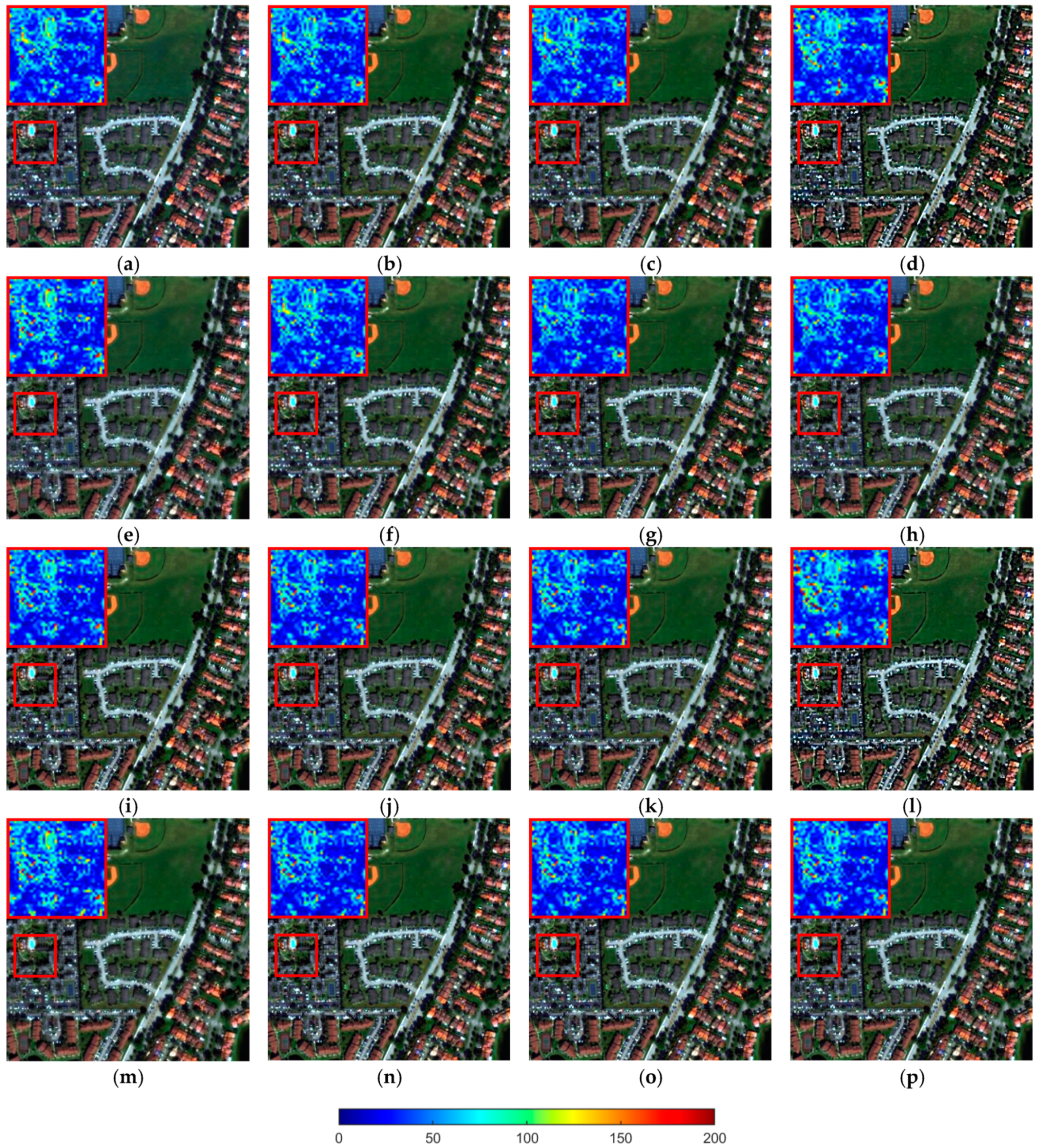
Figure 3 shows the comparison of the sum of squared differences (SSD) between the reference image and the closed-form solution under both representations.
It can be clearly seen that the results based on the residual representation can greatly improve the error in the boundary parts of the image. It should be noted that the boundary error problem may also exist in the residual representation, and the degree of error is directly related to the setting of μ . A larger μ means a higher weight of the regular term and a smaller boundary error, but at the same time the difference with the BP objective function will be larger, which may cause a degradation of performance. With the same μ value setting, the results using the residual representation are always better than the results of the original image space representation. In fact, the boundary problem of sharpened results is common, for example, the most commonly used tap-23 filter also leads to some degree of boundary defects. Usually, a border crop is used by default (or a border padding) to remove the effect of this content. Therefore, the smaller the μ value, the more significant the performance improvement without affecting the boundary quality of the final output image. The residual representation can be more effective in reducing the reasonable range of μ values.
From the point of view of optimization objectives, (32) can also be understood as adding Tikhonov regularization (Tikhonov matrix is I ) on the basis of the original data fidelity term on residuals, thereby replacing ( M G T M G ) 1 with ( M G T M G + μ I ) 1 during the derivative calculation. Since this process only adds a small perturbation μ to the diagonal elements of the latter, it means that the impact on the original objective function is relatively small. At the same time, the original information of x 0 is also retained outside the optimization problem and will not change with the optimization process, which is equivalent to the implicit inclusion of the initial solution in the gradient descent method. It is worth mentioning that the practice of using residual representation to improve performance is also widely used in deep convolutional network design. Although the starting point is different (the latter is used to improve the vanishing gradient phenomenon and increase the depth of the network), the basic logic in effect is the same.
B.
Introducing General Spatial Projection Filter and Step Factor into Closed-Form Solution
On the basis of (33), the relevant variables of the interpolation stage are replaced with the relevant variables of the spatial projection filter. That is, to replace M G T and K H T with W G and K P , respectively, the solution at this time is
r ^ x = 1 μ W G r S 1 μ W G F 1 F M G W G r S F h p ~ 0 + μ
where h p ~ 0 = F 1 F K H F K P · s .
Note that when K P = K u is the approximate ideal interpolation function mentioned earlier, and when K P = K H T is equivalent to the original closed-form solution corresponding to (33).
Different from (34), both (31) and (33) are derived from the derivation of the corresponding optimization objective functions. Due to the inclusion of M G T -related terms, the latter two match the degradation transpose BP in terms of idea and performance. However, the purpose of this section is to form a more accurate approximation to BP while accelerating. Since the projection filter of BP itself has no actual physical meaning, it can theoretically be set arbitrarily under the condition of convergence, and it does not rule out the possibility of a better choice than degradation transpose. For example, in addition to degradation transpose projection filters, projection filters based on ideal interpolation can also be used. The following is a further analysis of the two types of filters.
First, the difference between the two is in the “shape” of the filter, or more importantly, in the Nyquist frequency to which the two correspond. 
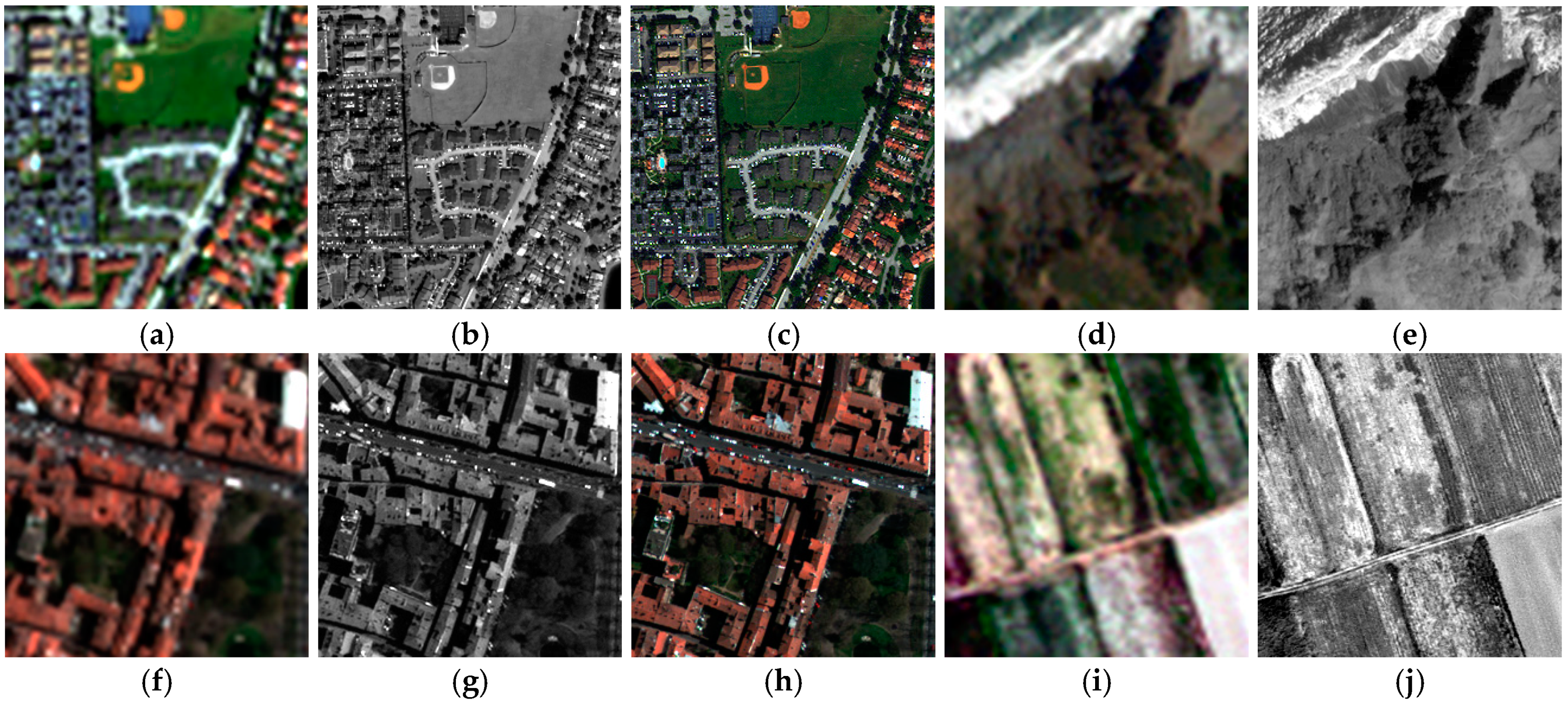
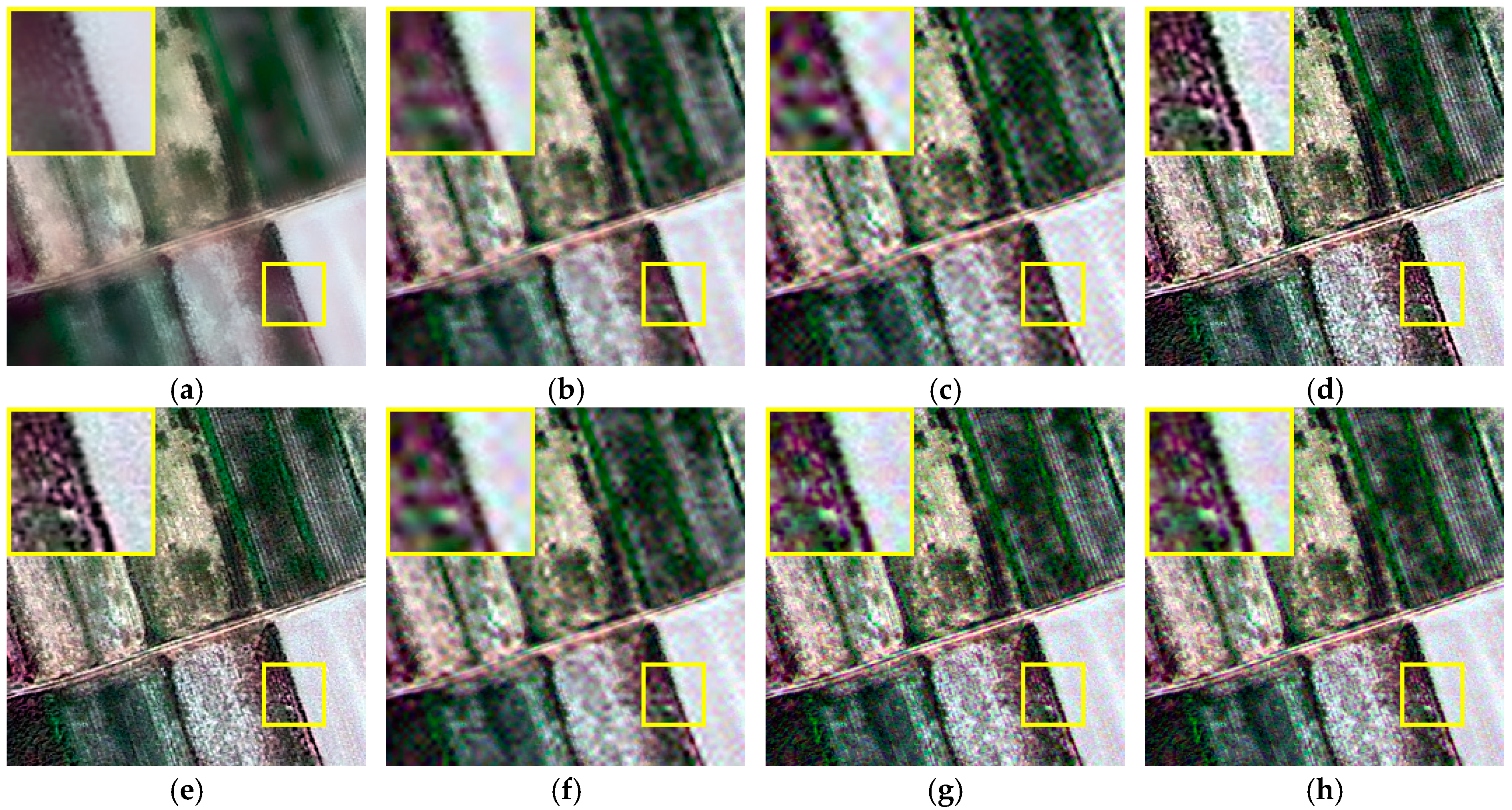
Figure 4 is an example of the interpolation results of the two filters, and the small picture in the upper left corner is the corresponding filter.
In principle, the interpolation process includes two stages of upsampling and low-pass filtering, wherein the purpose of the low-pass filtering operation is to remove the periodic repetition of the spectrum caused by the insertion of 0 samples in the upsampling stage. For digital images, approximate ideal interpolation functions (such as tap-23 commonly used for sharpening and tap-7 corresponding to bicubic) can make the image after the sampling rate increase as much as possible to keep the original signal samples unchanged. Intuitively speaking, the image should be enlarged to avoid blurring or other visual defects. The projection filter used in the degradation transpose BP is a K H adapted to the MTF of the MS sensor with a Nyquist frequency typically around 0.3. If it is used in the interpolation process, there will be a loss of high-frequency information compared to the ideal interpolation function with a Nyquist frequency of 0.5. It can be seen from Figure 4 that the result of the degenerate filter is slightly blurred compared to the ideal interpolation. Therefore, the ideal interpolation filter should be better than the degradation transpose filter in terms of interpolation principle. However, in terms of the entire BP process, the impact of this difference needs to be viewed dialectically. Considering that the projection operation is imposed on the error term e k λ in the BP process (see (6)), it means that in each iteration process, the residual term of the degradation transpose BP is slightly more blurred than that of the ideal interpolation BP. On the one hand, if the unique details contained in y M itself are not well preserved in x 0 (as is the case with many sharpening algorithms) or there is useful detail compensation information in e k λ due to the insufficient details injected by x 0 from y P , then the ideal interpolation BP will be more helpful to restore this part of detail than the “clear” e k λ . On the other hand, if y M or x 0 contains some unnecessary detail defects (such as noise or aliasing) and appears in e k λ , the relatively “fuzzy” e k λ of degradation transpose BP can filter this part of the content, and the ideal interpolated BP may amplify the influence of these defects.
Second, the difference between the two projection filters is also reflected in the scaling of the coefficients. As mentioned above, the conventional interpolation filter (used in the ideal interpolation BP) is for the purpose of preserving energy (see Section 3.3.2), and the sum of the coefficients is generally r 2 times that of the degradation filter. In contrast, there is no magnification scaling between the interpolation and degradation filters of the degradation transpose BP (i.e., the scaling is 1). However, this does not imply that the degradation transpose BP is defective in energy preservation. In fact, according to the BP iterative formula of (6), since the projection filter acts on the error e k λ , its coefficient magnification actually does not mainly involve the problem of maintaining the total energy of the image, but realizes the scaling of e k λ . It is equivalent to playing the role of the step size factor in the iterative process, that is, the default step size of the degradation transpose BP and the ideal interpolation BP is 1 and r 2 , respectively. In order to unify the operation between different filters and increase the variability, this paper further multiplies the closed-form solution of BP and the W G -related variable (i.e., K P -related) in the iterative formula by a normalized step-size factor γ n = γ / K P , i , where K P , i represents the accumulation of K P coefficients. For the Fast BP (FBP), that is, (34) is adjusted accordingly as
r ^ x = γ n μ W G r S γ n μ W G F 1 F γ n M G W G r S F γ n h p ~ 0 + μ
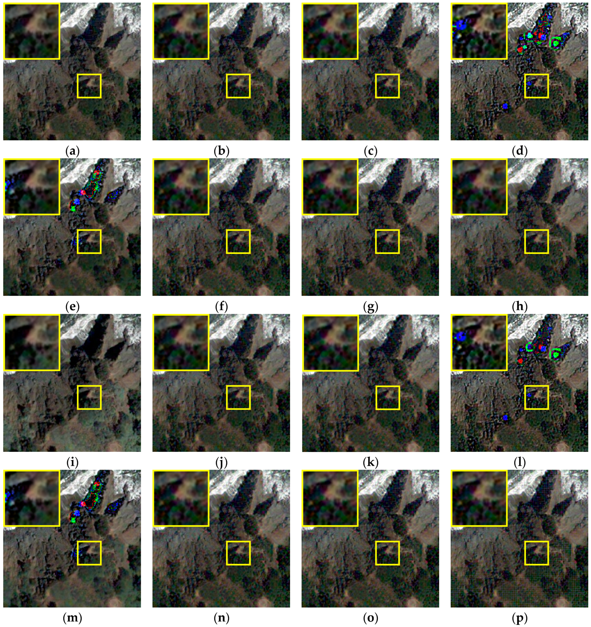
Figure 5 shows the iterative convergence of the two BPs with different step size factors.
From Figure 5, the following can be concluded:
(1) The effect of step size is consistent with the general iterative algorithm. The larger the step size, the faster the rate of residual decrease, but too large a step size may result in failure to obtain lower residuals or even non-convergence.
(2) The descent rate of the ideal interpolated BP is slightly higher than that of the degradation transpose BP when the same step factor is used and the convergence condition is satisfied, but the difference is not significant.
(3) The default step size of the degradation transpose BP ( γ = 1 ) cannot achieve a reasonable degree of convergence in a small number of iterations, while the step size of the ideal interpolation BP ( γ = 16 ) has the fastest convergence rate.
Therefore, combined with the consideration of the convergence conditions, the reasonable range of γ can be set to [ 1 , r 2 ] . Appropriately selecting a larger step size within a reasonable range is beneficial to obtain better comprehensive performance.
With the introduction of the step size factor, it is also equivalent to further increasing the variability of the projection filter settings. This is because the filters corresponding to different step sizes can be considered different (although only degenerate and ideal interpolation filter “shapes” are considered in this paper). Although the generic projection filter setting can no longer be derived from the optimal objective function, the modified solution is better suited from the point of view of finding a non-iterative fast solution that is as consistent as possible with the BP algorithm. Further change to other shapes of arbitrary filters satisfying the convergence condition is possible according to the actual demand.

3.5.2. Fast SSBP

The derivation process of FSSBP is similar to that of FBP, with the difference being the addition of spatial consistency-related content. Its corresponding objective function containing spatial, spectral fidelity and regular terms is as follows:
a r g m i n x { M G x y M 2 2 + σ 2 M R x y P 2 2 + μ 2 x x 0 2 2 }  
Similarly, although the closed-form solution of (36) cannot be obtained by direct derivation, it has been studied by sharpening the related literature in recent years. Qi et al. [28,34] organized the equation obtained from the derivation under the objective problem of matrix representation into the form of the Sylvester equation and gave two proof ideas successively by exploring the structural characteristics of the coefficients of the matrix in question in the frequency domain and introducing auxiliary matrix operations for simplification. The first idea is based on the direct derivation of HR scale (corresponding to M G T M G ). The second idea is similar to that in the aforementioned literature [30,33], using the inversion formula to convert the subsequent derivation to the LR scale, which improves the robustness of the method.
By comparing the proof ideas of [30,34], this paper replaces the relevant part of the convolution operation involved in the closed-form solution with the following more concise representation:
x ^ = Q 1 λ c b x γ n λ c W G F 1 F M G b x F γ n h p ~ 0 + λ c
among them, b x = Q 1 ( γ n W G y M + σ W R y P + μ x 0 ) , Q and λ c are obtained by eigenvalue decomposition of c = σ W R M R + μ I , that is, c = Q Λ c Q 1 , and λ c is a vector composed of Λ c diagonal elements.
Further, in order to replace (37) with the residual representation, (36) is first replaced with the following objective function:
r ^ x = a r g m i n x { M G r x r S 2 2 + σ 2 M R r x r λ 2 2 + ρ 2 r x 2 2 }
where r λ = y P M R x 0 .
The corresponding closed-form solution of (38) is
r ^ x = Q 1 λ c b r γ n λ c W G F 1 F M G b r F γ n h p ~ 0 + λ c
where b r = Q 1 ( γ n W G r s + τ W R r λ ) .
Compared with the original closed-form solution based on the full matrix implementation in [34], the advantage of the modified closed-form solution is that it is easier to understand, and the memory overhead is significantly reduced because it does not need to store many high-dimensional matrices. In addition, the original closed-form solution is derived with a default sampling offset of (0, 0), which is inconsistent with the actual situation in most datasets. Although it can be solved by translating the input image, it may cause a certain degree of quality degradation. In contrast, the convolution-based solution can deal with this problem in a more natural way. The two closed-form solutions are essentially identical in terms of computational efficiency.

4. Experiments and Analysis

4.1. Dataset and Experimental Setup

In order to verify the effectiveness of the proposed method, a total of four sets of data consisting of different scene types and remote sensing platforms are selected for experiments under degradation scale (DS) and full scale (FS) in this paper. Among them, DS experiments are subdivided into full and half simulations according to whether they include both spatial and spectral degradation.
The data used are from publicly available sample images or code packages [35,36,37], and the relevant information is shown in Table 2. For display purposes, all images are cropped and linearly stretched as in [35], and the size of the cropped HR images is 256 × 256 pixels. The experimental images used are shown in Figure 6.
In terms of comparison algorithms, in addition to the original sharpened results (without post-processing), this paper selects degradation transpose BP (denoted as B P T ), ideal interpolation BP (denoted as B P I ), EBP [21] and BP-related post-processing methods of Jiao et al. (referred to as FE-BP) [22] to compare with the SSBP, FBP and FSSBP methods proposed in this paper, which make for a total of eight types of post-processing. Among them, EBP and FE-BP also focus on the improvement of BP spatial quality. Since each BP method can be applied to any sharpened results, in order to avoid unnecessary redundancy in the display of experimental content caused by the combination of different situations, the experiments in this paper are divided into two modes. First, on the first two sets of data, two specific sharpening methods are selected as the base methods for providing sharpening for the initial images, and combined with the above types of post-processing methods to carry out subjective visual quality comparisons and comparisons of multiple objective evaluation indicators, which is all together referred to as the “dual-base-multi-indicator” experiment. Secondly, on the latter two data, a single reference/non-reference evaluation indicator reflecting the comprehensive quality of sharpening is applied, and statistical comparisons based on multiple sharpening base methods are selected, and a statistical comparison based on multiple sharpening base methods is carried out, i.e., the “multi-base-single-indicator experiment”. The source code of the proposed method can be downloaded from https://github.com/JZ-Tao/FSSBP/ (accessed on 12 September 2023).

4.2. Parameter Setting

In terms of common parameters, the default settings are kept for all base methods. The number of iterations of all iterative BPs is fixed at 100. In terms of iteration step size, the default step size of B P I and B P T at a resolution ratio of 4 corresponds to a 16:1 relationship according to the previous discussion. Both FE-BP and EBP use B P T as the basic iterative optimization method, where EBP does not include a step size setting, while the beta parameter equivalent to the step size in FE-BP is set to 0.1, the same as in [22].
The parameter settings of the proposed methods are shown in Table 3. The spatial projection filters vary from data to data. It is clear from the later experiments that the results are relatively better when the ideal interpolation and degradation transpose projection filters are used on the DS data and FS data, respectively. The possible reason for this is that the DS data apply an additional filtering operation to the source image, which reduces the possible noise and aliasing and is thus more suitable for the ideal interpolation filter (corresponding to B P I ), while the FS data are more stable when using the relatively “safe” degradation transpose filter (corresponding to B P T ). Similar to the spatial projection filter, the spectral projection in SSBP and FSSBP gives relatively better results using the Gram–Schmidt (GS) transform and degradation transpose approaches for the DS and FS data, respectively. For the step-size setting, according to the analysis of Figure 5, the step size γ of SSBP is set to 16 to obtain relatively good performance. For FBP and FSSBP, γ has an overall inverse relationship with the regularization parameter μ . Unlike the iterative type of BP methods that lead to the non-convergence of results when the step size is too large (e.g., more than 24), there is no specific range of valid values for γ in the fast method under the influence of μ . To be consistent with SSBP, γ is also set to 16 for both. Regarding the setting of μ , the smaller μ is usually closer to the quality of the corresponding iterative BP for each of the two, but too small a value of μ may lead to the non-convergence of the results. The optimal μ value may vary slightly depending on the data and experiment type, and is fixed to 0.0098 and 0.2 for DS and FS experiments, respectively. For the spatial error term weights τ of SSBP and FSSBP, similar to μ , are set to 0.1 and 1 in the DS and FS experiments, respectively.

4.3. Dual-Base-Multi-Indicator Experiment

In this set of experiments, consistent with the general sharpening evaluation approach, the quality of the results is comprehensively reflected by using multiple evaluation indexes [38,39]. The base methods used for the D-WV data were selected as PNN (pan-sharpening neural network) [36] and STEM-MA (shearlet transform-based entropy matching with mode addition) [40]. The former is a novel DL-based method, which is one of the state-of-the-art methods. The latter is a recently proposed hybrid method. SAM, ERGAS, RMSE, SSIM and Q2n [41] were selected as evaluation metrics for DS experiments.
The base methods used for F-QB data were selected as GLP and GS methods, both of which are representative methods in the MRA and CS categories, respectively, and the two methods selected as base methods in [20]. HQNR [42], QNR+ [43], and Consistency-based Q2n (C-Q2n) [44] were selected as evaluation metrics for FS experiments. By convention, the spectral loss metric D λ K [42] and the spatial loss metrics D S [12], and D S R 2 [43], which constitute the first two comprehensive evaluation metrics in the QNR category, are also listed together. The definitions of the evaluation metrics in the DS and FS experiments are shown in Table 4.

4.3.1. DS Experiment: D-WV Data

Figure 7 and Table 5 correspond to the sharpened image of the data D-WV and the quantitative evaluation results with reference, respectively. The small image corresponding to the upper left corner of Figure 7 is the SSD image relative to the reference image, corresponding to the delineated area and is enlarged (2.5 times). In Table 5 (and also in Table 6, Table 7 and Table 8 below), for each type of evaluation index, the best and second best index values corresponding to each base method are highlighted using the font styles of “bold” and “underline”, respectively.
From the SSD maps in the upper left corner of Figure 7a,i, it can be seen that the initial results obtained by STEM-MA have a slightly smaller SSD error than PNN in the corresponding region. By comparing the raw sharpened result metrics of PNN and STEM-MA in Table 5, it can be seen that PNN has an advantage in terms of spectral quality (lower SAM), but the rest of the metrics are slightly inferior to STEM-MA. The ERGAS and Q2n metrics, which can comprehensively reflect the sharpened quality of both, are relatively close to each other—which is the reason for comparing them as base methods.
After optimization via different BP methods, it can be seen from Figure 7 that except for the EBP results, which are obviously sharper, the overall visual quality change in the original sharpened results by other optimization methods is not easily detectable, and basically only some differences can be observed in the SSD maps. In the PNN group (Figure 7a–h), by comparing the error concentration area in the upper left part of each SSD map, it can be found that the Figure 7g,h plots corresponding to SSBP and FSSBP have the largest improvement. The Figure 7b,c,f maps corresponding to GS, BPI and FBP are almost identical visually. Figure 7e corresponding to FE-BP is slightly blurred in general compared to the original result, and although some of the error locations in its SSD map are somewhat improved, new errors are introduced at other locations. In the STEM-MA group (Figure 7i–p), the trends of EBP and FE-BP remain consistent with the PNN group, with the difference that the other methods correspond to a less pronounced degree of perceptible change in the SSD maps. This indicates that PNN should improve more than STEM-MA with the same optimization method (except the method that brings negative optimization).
As can be seen from Table 5, the optimization results obtained by SSBP outperform the other comparison methods in all metrics except SAM, which is slightly weaker due to the fact that the optimization objective of the method is not solely aimed at spectral quality improvement. The performance of the two accelerated methods (FSSBP and FBP) is slightly inferior to their corresponding iterative versions in general due to the use of regularization to form approximate solutions, but their SAMs are further improved. FSSBP is basically better than the other compared methods in terms of overall performance, and is second only to SSBP. Compared with BPT, BPI has a slight advantage in these data.
The quantitative evaluation values of EBP showed a large degree of recession compared to the original results under some indicators such as ERGAS. The enhancement idea of the method is to use the multiplicative rule of the GLP-HPM method for the initial results to extract details from the PAN again and inject them, and its effectiveness depends on the spatial quality of the adopted base method and the chosen enhancement method (i.e., HPM) itself. For a sharpened result with sufficient detail information, this process will lead to an over-injection of details. For a sharpened result with insufficient detail, however, the process does not preclude the ability to supplement the detail appropriately. For example, if direct interpolation is used as the initial result and then enhanced with EBP, the output will be equivalent to the sharpened result of the GLP-HPM method. While very sharp results may be more advantageous in some visualization applications, they are inconsistent with the rating of integrated spatial–spectral quality that is commonly sought in sharpening applications.
Also employing a GLP-HPM related method, FE-BP’s enhancement scheme for the initial results is to keep their low frequencies and replace their high frequencies with the high frequencies of the HPM results (more specifically, the FE-HPM method). In sharpening applications, the enhancement logic of this method is relatively reasonable compared to EBP, but this replacement process implies the assumption that the high frequencies of the FE-HPM method should be more accurate than the high frequencies of the sharpened initial results, i.e., its effectiveness also depends heavily on the enhancement method itself. As can be seen from the table, FE-BP yields weaker results than the original BP, and also brings a small amount of negative optimization. In addition to the possible influence of the accuracy of the blurred kernel estimation, this result should be attributed more to the fact that the chosen base method corresponds to a better spatial quality of the initial results than FE-HPM.
Overall, PNN obtains more effective quality improvement than STEM-MA after the same optimization method, in agreement with the analysis above. The possible reason is that STEM-MA has introduced spatial consistency considerations in its scheme design through spectral transformations, and is therefore less affected by the spatial–spectral optimization method proposed in this paper.

4.3.2. FS Experiment: F-QB Data

Figure 8 and Table 6 correspond to the sharpened images of the F-QB data and the quantitative evaluation results without reference, respectively. The small picture in the upper left corner of Figure 8 is the enlarged result of the image of the delineated area.
From Figure 8, we can clearly see the defects of EBP and FE-BP methods affected by the instability of the multiplicative rule value of GLP-HPM method itself; at the position containing dark pixels (such as the mountain range of the enlarged part in Figure 8a–h), it is easy to cause abnormal results because the value of the divisor is too small relative to the divisor, resulting in significant color patches in Figure 8d,e,l,m. In fact, replacing the HPM method used by both with a fog-corrected HPM method (i.e., GLP-HPM-H) [45,46] is expected to improve this defect relatively effectively. The rest of the optimized results for the GLP group are also very close to the original GLP results (Figure 8a). It can be seen from the previous experimental analysis that this means that the original quality of the GLP method is higher. However, compared with the (Figure 8b) picture of BPT, the (Figure 8c) picture of BPI shows a little aliasing phenomenon (sawtooth effect) from the wave part in the upper left corner, especially near the coastline, which means the visual quality of BPI is weaker than BPT. The results of FBP are close to BPT; FSSBP and SSBP repair the aliasing phenomenon.
For the GS group, except for the same parts as those observed above, it can be seen from the enlarged part of Figure 8i of the original results that it has obvious spectral distortion (the vegetation color is lighter). Thanks to the optimization of BP, all optimization methods (Figure 8j–p) can effectively improve this phenomenon.
The following can be seen from Table 6: Consistent with the DS experiments in the previous subsection, the two BP original algorithms that focus on improving spectral consistency have the least spectral distortion (the lowest D λ K value and the highest C-Q2n). Compared with BPT, although BPI obtains a lower D λ K value due to the larger equivalent step size, its comprehensive evaluation is weaker than that of BPT due to the influence of space quality, which is consistent with the observation results; HQNR, as a hybrid indicator that has been considered to replace QNR in recent years [37], has been experimentally found that the weights of its spatial ( D S ) and spectral ( D λ K ) evaluations are often different. Generally speaking, the magnitude of D λ K is lower than that of D S , which means that this indicator is more inclined to maintain spectral consistency. When the spatial consistency is introduced, the D S index has a certain degree of design rationality problem [44] (FE-BP is sub-optimal under this indicator, but it has obvious quality defects from the sharpened results), which leads to an increase in the D λ K error caused by adjusting the corresponding parameters, while the D S does not obtain a corresponding degree of decline. Therefore, the proposed spatial–spectral consistency method fails to obtain a good evaluation under this index; under the QNR+ index, SSBP and FSSBP were optimal and sub-optimal, respectively, and the numerical differences were not obvious, especially in the GLP group. Although Q2n can maintain good stability under different scale experiments [47], the C-Q2n index is also inclined to the evaluation of spectral preservation according to its principle, and cannot well reflect the spatial quality difference of HR scale, and the distinguishability between values is not good (for example, the indicators of GLP and GS after BPI processing are both 1).Therefore, also as a comprehensive performance evaluation index, it can be seen from the comparative analysis of the numerical values in the table and the results in Figure 8 and the consistency comparison with the DS experimental evaluation, compared with HQNR and C-Q2n, QNR+ can more reasonably reflect the spatial–spectral performance of each method under FS experiments.

4.4. Multi-Base-Single-Indicator Experiment

In the previous experiment, one of the base methods from the new type, the MRA-CS hybrid, the MRA, and the CS class was selected for analysis. The experiments in this section further expand the number of base methods belonging to the above four categories to 18 (since PNN does not provide a network model adapted to the Pléiades sensor, it is excluded from the D-PL data experiment. For similar situations, see [21].), in order to verify the generality of the proposed method for different base methods.
The selected base methods include (i) CS: BDSD-PC [48], BT-H [43], GS [49], GSA, NL-IHS [50], and PRACS [51]; (ii) MRA: ATWT-M3 [52], Indusion [53], GLP, GLP-HPM-H, and REG-GLP [54]; (iii) hybrid: AWLP-H, GFPCA [55], STEM-MA and STEM-MS [40]; (iv) new type: PNN [36], PWMBF [56], and SR-D [57]. The code implementations of the above base methods, except STEMs, are from the “Open Remote Sensing” website (https://openremotesensing.net/kb/codes/, accessed on 12 September 2023). These methods include both newly proposed methods with leading performance in recent years and some classical methods that are considered less competitive. For the comparison of visual effects, since the case of high-quality base methods was shown in the previous section, the classical ATWT-M3 and GFPCA are selected as the base methods for each of the D-PL and F-GE data to avoid content redundancy, where the former tends to obtain relatively blurred spatial quality and the latter is usually not superior in terms of both spatial and spectral quality. In terms of evaluation metrics, Q2n and QNR+, which better reflect the comprehensive performance, are selected for D-PL and F-GE, respectively. The visual display and evaluation results of the D-PL data are shown in Figure 9 and Table 7, respectively, and the small image in the upper left corner is the SSD map. The corresponding results of the F-GE data are shown in Figure 10 and Table 8, respectively, and the upper left corner is the partially enlarged result.
From a comprehensive comparison of Figure 9 and Figure 10, it can be clearly seen that EBP, FE-BP, SSBP and FSSBP have the ability to repair image spatial quality. In contrast, BPT, BPI, and FBP have limited repair effects. For BPI and BPT, both still have relative advantages in DS and FS experiments, but the advantage of BPI is not obvious; on the contrary, it has a serious aliasing problem under the FS experiment (Figure 10c). Although the results are still slightly blurred, from the SSD maps in Figure 9b,c,f, the improvement effect of the three original BP methods is still better than that of EBP and FE-BP. Compared with other methods, the over-sharpening problem of EBP still exists, but the degree is not so obvious because the initial results are relatively blurred, especially under the F-GE data, which are very close to the results of FE-BP visually, only slightly sharper than the latter. The results of SSBP and FSSBP are almost the same, which is still superior to other methods. In the D-PL data, it can be seen from the SSD map comparison that in the F-GE data, although the four spatially enhanced BP methods are close in sharpness, spectral distortions appear in EBP and FE-BP (the overall color shift green), which is caused by the HPM method itself.
In terms of the comparison of evaluation indicators of multiple base methods, it can be seen from Table 7 that various base methods have obtained the most and second most performance improvements under SSBP and FSSBP, respectively, which are almost the same. This is followed by BPI, BPT, FBP and FE-BP. EBP is negatively optimized for most of the methods, except for the relatively weak base method. The effectiveness of this method is uncertain; for example, the degree of optimization varies greatly for two methods, ATWT-M3 and Indusion, which belong to the same MRA category and have close Q2n metrics in the original results. Some base methods with excellent spatial quality proposed in recent years (e.g., BT-H, GLP-REG, etc.) can also obtain good optimization results using only BP, and most of these methods belong to the CS or hybrid classes that originally already include the consideration of spatial consistency. The optimization effect with the original BP (or FBP) after further introduction of spatial consistency (i.e., SSBP and FSSBP) is basically the same or has only a negligible quality reduction. In fact, it is found that for the above base method, the case corresponding to an optimal τ value of 0 (i.e., no spatial error term is introduced) is not fixed but may occur for some combinations of the base-method data-experiment types. On the one hand, if the base method already includes spatial consistency considerations, the additional introduction of the spatial error term may instead reduce the correction ratio of the spectral error. On the other hand, it is also related to the spatial–spectral tendency of the comprehensive evaluation index. For FS (or DS) experiments, the best choice of τ value is usually either 0 or 1 (or 0.1). Then in FSSBP, thanks to its fast computational process, the following adaptive τ setting can be considered further based on the above analytical choice: the FSSBP results under τ = 0 and τ = 1 (or 0.1) are calculated separately, and then the more optimal solution is selected according to QNR+. For simplicity, a fixed τ value setting is used in this paper.
The statistics of the mean and average rate of change in Table 8 corresponding to the F-GE data show that for all the chosen base methods, the improvement of FSSBP and SSBP compared to the other methods is more pronounced than in Table 7, corresponding to the D-PL data. SSBP is slightly better than FSSBP, but the actual visual difference is almost imperceptible. At the same time, the indicator values of FBP and its corresponding BPT are very close, and most of the base methods are even slightly better than the latter. Affected by aliasing, BPI also has more negative optimizations in this group of experiments. The ranking of quality improvement is in the order of SSBP, FSSBP, FBP, BPT, FE-BP, BPI and FBP. The rest of the experimental findings are basically the same as those described above and will not be repeated here.
By summarizing the above two sets of experiments, it can be seen that the fast method proposed in this paper can form a sufficiently effective high-precision approximation for BP and SSBP. In addition, by comparing the evaluation values before and after optimization, it can be found that the base method with good initial results can usually obtain relatively better optimization results, but this conclusion is not strictly established. Some methods that are usually considered obsolete or perform relatively poorly with certain data have the potential to outperform some methods that are considered to possess higher quality, such as GS compared to GSA, after being optimized by the method proposed in this paper.

4.5. Computation Time Comparison

This section further presents the calculation time comparison of several post-processing optimization methods. A total of three different image sizes are tested for the calculation time, and the average value is obtained by executing each method 10 times in a row. The parameter settings of each method are consistent with the above experiments. Note that the calculation time results include only the post-processing stage and do not include the calculation time of the base method, and are independent of the type of base method and the selection of specific data. The experimental platform used is Windows 10 + Intel i5-7200U @2.50GHz + MATLAB R2019b. The results are shown in Table 9.
From Table 9, it can be seen that the calculation time of each iterative method except the two fast methods and FE-BP is basically at the same level. The reason why FE-BP has an advantage in computing time compared to other iterative BP methods is that the size of the convolution kernel estimated by the filter estimation method is set to be smaller than the default high-precision MTF convolution kernel (the former has a length of 25, the latter is 41). From the above statistics, it is clear that reducing the size of the convolution kernel is also an effective way to reduce the computational time complexity. Although the relevant conclusions are not mentioned in the original literature of the FE-BP method, from the experimental results, this paper believes that this is actually the most obvious advantage when replacing the default convolution kernel with the estimated convolution kernel. Finally, the computational efficiency of the two fast methods is much better than any of the iterative methods involved in the comparison. Overall, FSSBP slightly increases computation time compared to FBP, but the difference is small. The experimental findings can be consistent at different scales. For FSSBP, the speedup relative to SSBP at the tested parameters is at least 27.5.

5. Conclusions

In this paper, a general post-processing optimization study for pan-sharpening methods is carried out based on BP with the MRA method as the analytical entry point for the problem that the spectral consistency condition is commonly not satisfied. First, the concept of spatial consistency is introduced and used to characterize the spectral degradation relationship between MS and PAN images, and the corresponding spatial–spectral BP method, i.e., the SSBP method, is proposed. Further, the convergence condition of the proposed method and the proof of the convergence condition for the more relaxed BP of the degradation transpose are given. Finally, the corresponding non-iterative methods, namely the FBP and FSSBP methods, are proposed for BP and SSBP, and effective improvements are formed by introducing residual representations and generalized projection filters in the closed-form solutions concerned. It is experimentally demonstrated that the proposed SSBP method can form a general spatial–spectral consistency improvement on the sharpened results. The computational efficiency of the proposed fast method is significantly improved compared to the corresponding iterative version while the optimization quality is close to or only slightly degraded.

Author Contributions

Formal analysis and writing—original draft preparation, J.T.; Data curation, Writing—review and editing, W.N.; Investigation validation, C.S.; Conceptualization and methodology, X.W.; All authors have read and agreed to the published version of the manuscript.

Funding

This research was funded by the National Natural Science Foundation of China (Grant No. 42371338).

Data Availability Statement

The data used in this paper can be downloaded from https://github.com/JZ-Tao/FSSBP/ (accessed on 12 September 2023).

Acknowledgments

The authors would like to thank Wanfeng Qi from the School of Mathematics, Liaoning Normal University for his helpful discussions on the relevant content of this paper and the editors and the reviewers for their valuable suggestions.

Conflicts of Interest

The authors declare no conflict of interest.

References

  1. Shaw, G.A.; Burke, H.-H.K. Spectral imaging for remote sensing. Linc. Lab. J. 2003, 14, 3–28. [Google Scholar]
  2. Javan, F.D.; Samadzadegan, F.; Mehravar, S.; Toosi, A.; Khatami, R.; Stein, A. A review of image fusion techniques for pan-sharpening of high-resolution satellite imagery. ISPRS J. Photogramm. Remote Sens. 2021, 171, 101–117. [Google Scholar] [CrossRef]
  3. Wang, Y.; Shao, Z.; Lu, T.; Wu, C.; Wang, J. Remote Sensing Image Super-Resolution via Multiscale Enhancement Network. IEEE Geosci. Remote Sens. Lett. 2023, 20, 3248069. [Google Scholar] [CrossRef]
  4. Vivone, G.; Mura, M.D.; Garzelli, A.; Restaino, R.; Scarpa, G.; Ulfarsson, M.O.; Alparone, L.; Chanussot, J. A new benchmark based on recent advances in multispectral pansharpening: Revisiting pansharpening with classical and emerging pansharpening methods. IEEE Geosci. Remote Sens. Mag. 2021, 9, 53–81. [Google Scholar] [CrossRef]
  5. Stankevich, S.A.; Piestova, I.O.; Lubskyi, M.S. Remote sensing imagery spatial resolution enhancement. In Recognition and Perception of Images: Fundamentals and Applications; Wiley: Hoboken, NJ, USA, 2021; pp. 327–367. [Google Scholar]
  6. Meng, X.; Xiong, Y.; Shao, F.; Shen, H.; Sun, W.; Yang, G.; Yuan, Q.; Fu, R.; Zhang, H. A large-scale benchmark data set for evaluating pansharpening performance: Overview and implementation. IEEE Geosci. Remote Sens. Mag. 2020, 9, 18–52. [Google Scholar] [CrossRef]
  7. Wald, L.; Ranchin, T.; Mangolini, M. Fusion of satellite images of different spatial resolutions: Assessing the quality of resulting images. Photogramm. Eng. Remote Sens. 1997, 63, 691–699. [Google Scholar]
  8. Yokoya, N.; Grohnfeldt, C.; Chanussot, J. Hyperspectral and multispectral data fusion: A comparative review of the recent literature. IEEE Geosci. Remote Sens. Mag. 2017, 5, 29–56. [Google Scholar] [CrossRef]
  9. Meng, X.; Shen, H.; Li, H.; Zhang, L.; Fu, R. Review of the pansharpening methods for remote sensing images based on the idea of meta-analysis: Practical discussion and challenges. Inf. Fusion 2019, 46, 102–113. [Google Scholar] [CrossRef]
  10. Tsagkatakis, G.; Aidini, A.; Fotiadou, K.; Giannopoulos, M.; Pentari, A.; Tsakalides, P. Survey of deep-learning approaches for remote sensing observation enhancement. Sensors 2019, 19, 3929. [Google Scholar] [CrossRef]
  11. Vivone, G.; Alparone, L.; Garzelli, A.; Lolli, S. Fast reproducible pansharpening based on instrument and acquisition modeling: AWLP revisited. Remote Sens. 2019, 11, 2315. [Google Scholar] [CrossRef]
  12. Alparone, L.; Aiazzi, B.; Baronti, S.; Garzelli, A. Remote Sensing Image Fusion; CRC Press: Boca Raton, FL, USA, 2015. [Google Scholar]
  13. Garzelli, A. A review of image fusion algorithms based on the super-resolution paradigm. Remote Sens. 2016, 8, 797. [Google Scholar] [CrossRef]
  14. Vivone, G.; Marano, S.; Chanussot, J. Pansharpening: Context-based generalized Laplacian pyramids by robust regression. IEEE Trans. Geosci. Remote Sens. 2020, 58, 6152–6167. [Google Scholar] [CrossRef]
  15. Starck, J.-L.; Fadili, J.; Murtagh, F. The undecimated wavelet decomposition and its reconstruction. IEEE Trans. Image Process. 2007, 16, 297–309. [Google Scholar] [CrossRef]
  16. Kallel, A. MTF-adjusted pansharpening approach based on coupled multiresolution decompositions. IEEE Trans. Geosci. Remote Sens. 2015, 53, 3124–3145. [Google Scholar] [CrossRef]
  17. Zhang, H.K.; Huang, B. A new look at image fusion methods from a bayesian perspective. Remote Sens. 2015, 7, 6828–6861. [Google Scholar] [CrossRef]
  18. Hallabia, H.; Kallel, A.; Hamida, A.B. A remote sensing fusion approach using MTF-adjusted filter banks. In Proceedings of the 2016 2nd International Conference on Advanced Technologies for Signal and Image Processing (ATSIP), Monastir, Tunisia, 21–23 March 2016; pp. 505–510. [Google Scholar]
  19. Delleji, T.; Kallel, A.; Hamida, A.B. Iterative scheme for MS image pansharpening based on the combination of multi-resolution decompositions. Int. J. Remote Sens. 2016, 37, 6041–6075. [Google Scholar] [CrossRef]
  20. Vicinanza, M.R.; Restaino, R.; Vivone, G.; Mura, M.D.; Licciardi, G.A.; Chanussot, J. A method for improving the consistency property of pansharpening algorithms. In Proceedings of the 2014 IEEE Geoscience and Remote Sensing Symposium, Quebec City, QC, Canada, 13–18 July 2014; pp. 2534–2537. [Google Scholar]
  21. Liu, J.; Ma, J.; Fei, R.; Li, H.; Zhang, J. Enhanced back-projection as postprocessing for pansharpening. Remote Sens. 2019, 11, 712. [Google Scholar] [CrossRef]
  22. Jiao, J.; Wu, L. Image restoration for the MRA-based pansharpening method. IEEE Access 2020, 8, 13694–13709. [Google Scholar] [CrossRef]
  23. Vivone, G.; Simões, M.; Mura, M.D.; Restaino, R.; Bioucas-Dias, J.M.; Licciardi, G.A.; Chanussot, J. Pansharpening based on semiblind deconvolution. IEEE Trans. Geosci. Remote Sens. 2015, 53, 1997–2010. [Google Scholar] [CrossRef]
  24. Irani, M.; Peleg, S. Motion analysis for image enhancement: Resolution, occlusion, and transparency. J. Vis. Commun. Image Represent. 1993, 4, 324–335. [Google Scholar] [CrossRef]
  25. Dai, S.; Han, M.; Wu, Y.; Gong, Y. Bilateral back-projection for single image super resolution. In Proceedings of the 2007 IEEE International Conference on Multimedia and Expo, Beijing, China, 2–5 July 2007; pp. 1039–1042. [Google Scholar]
  26. Aiazzi, B.; Baronti, S.; Selva, M. Improving component substitution pansharpening through multivariate regression of MS+Pan data. IEEE Trans. Geosci. Remote Sens. 2007, 45, 3230–3239. [Google Scholar] [CrossRef]
  27. Horn, R.A.; Johnson, C.R. Matrix Analysis; Cambridge University Press: New York, NY, USA, 2012. [Google Scholar]
  28. Wei, Q. Bayesian Fusion of Multi-Band Images: A Powerful Tool for Super-Resolution. Ph.D. Thesis, Institut National Polytechnique de Toulouse (INPT), University Toulouse, Toulouse, France, 2015. [Google Scholar]
  29. Aiazzi, B.; Baronti, S.; Selva, M.; Alparone, L. Bi-cubic interpolation for shift-free pan-sharpening. ISPRS J. Photogramm. Remote Sens. 2013, 86, 65–76. [Google Scholar] [CrossRef]
  30. Chan, S.H.; Wang, X.; Elgendy, O.A. Plug-and-play ADMM for image restoration: Fixed-point convergence and applications. IEEE Trans. Comput. Imag. 2017, 3, 84–98. [Google Scholar] [CrossRef]
  31. Loncan, L.; Almeida, L.B.; Bioucas-Dias, J.M.; Briottet, X.; Chanussot, J.; Dobigeon, N.; Fabre, S.; Liao, W.; Licciardi, G.A.; Simões, M.; et al. Hyperspectral pansharpening: A review. IEEE Geosci. Remote Sens. Mag. 2015, 3, 27–46. [Google Scholar] [CrossRef]
  32. Yang, J.; Wright, J.; Huang, T.S.; Ma, Y. Image super-resolution via sparse representation. IEEE Trans. Image Process. 2010, 19, 2861–2873. [Google Scholar]
  33. Zhao, N.; Wei, Q.; Basarab, A.; Dobigeon, N.; Kouamé, D.; Tourneret, J.-Y. Fast single image super-resolution using a new analytical solution for ℓ2–ℓ2 problems. IEEE Trans. Image Process. 2016, 25, 3683–3697. [Google Scholar] [CrossRef]
  34. Wei, Q.; Dobigeon, N.; Tourneret, J.-Y.; Bioucas-Dias, J.; Godsill, S. R-FUSE: Robust fast fusion of multiband images based on solving a Sylvester equation. IEEE Signal Process. Lett. 2016, 23, 1632–1636. [Google Scholar] [CrossRef]
  35. Vivone, G.; Alparone, L.; Chanussot, J.; Mura, M.D.; Garzelli, A.; Licciardi, G.; Restaino, R.; Wald, L. A critical comparison among pansharpening algorithms. IEEE Trans. Geosci. Remote Sens. 2015, 53, 2565–2586. [Google Scholar] [CrossRef]
  36. Masi, G.; Cozzolino, D.; Verdoliva, L.; Scarpa, G. Pansharpening by convolutional neural networks. Remote Sens. 2016, 8, 594. [Google Scholar] [CrossRef]
  37. Vivone, G.; Dalla Mura, M.; Garzelli, A.; Pacifici, F. A benchmarking protocol for pansharpening: Dataset, preprocessing, and quality assessment. IEEE J. Sel. Top. Appl. Earth Obs. Remote Sens. 2021, 14, 6102–6118. [Google Scholar] [CrossRef]
  38. Alcaras, E.; Parente, C. The Effectiveness of Pan-Sharpening Algorithms on Different Land Cover Types in GeoEye-1 Satellite Images. J. Imaging 2023, 9, 93. [Google Scholar] [CrossRef] [PubMed]
  39. Wu, Y.; Feng, S.; Lin, C.; Zhou, H.; Huang, M. A Three Stages Detail Injection Network for Remote Sensing Images Pansharpening. Remote Sens. 2022, 14, 1077. [Google Scholar] [CrossRef]
  40. Tao, J.; Song, C.; Song, D.; Wang, X. Pan-sharpening framework based on multiscale entropy level matching and its application. IEEE Trans. Geosci. Remote Sens. 2022, 60, 3198097. [Google Scholar] [CrossRef]
  41. Garzelli, A.; Nencini, F. Hypercomplex quality assessment of multi/hyperspectral images. IEEE Geosci. Remote Sens. Lett. 2009, 6, 662–665. [Google Scholar] [CrossRef]
  42. Khan, M.M.; Alparone, L.; Chanussot, J. Pansharpening quality assessment using the modulation transfer functions of instruments. IEEE Trans. Geosci. Remote Sens. 2009, 47, 3880–3891. [Google Scholar] [CrossRef]
  43. Alparone, L.; Garzelli, A.; Vivone, G. Spatial consistency for full-scale assessment of pansharpening. In Proceedings of the IGARSS 2018—2018 IEEE International Geoscience and Remote Sensing Symposium (IGARSS), Valencia, Spain, 22–27 July 2018; pp. 5132–5134. [Google Scholar]
  44. Palsson, F.; Sveinsson, J.R.; Ulfarsson, M.O.; Benediktsson, J.A. Quantitative quality evaluation of pansharpened imagery: Consistency versus synthesis. IEEE Trans. Geosci. Remote Sens. 2015, 54, 1247–1259. [Google Scholar] [CrossRef]
  45. Lolli, S.; Alparone, L.; Garzelli, A.; Vivone, G. Haze correction for contrast-based multispectral pansharpening. IEEE Geosci. Remote Sens. Lett. 2017, 14, 2255–2259. [Google Scholar] [CrossRef]
  46. Garzelli, A.; Aiazzi, B.; Alparone, L.; Lolli, S.; Vivone, G. Multispectral pansharpening with radiative transfer-based detail-injection modeling for preserving changes in vegetation cover. Remote Sens. 2018, 10, 1308. [Google Scholar] [CrossRef]
  47. Carla, R.; Santurri, L.; Aiazzi, B.; Baronti, S. Full-scale assessment of pansharpening through polynomial fitting of multiscale measurements. IEEE Trans. Geosci. Remote Sens. 2015, 53, 6344–6355. [Google Scholar] [CrossRef]
  48. Vivone, G. Robust band-dependent spatial-detail approaches for panchromatic sharpening. IEEE Trans. Geosci. Remote Sens. 2019, 57, 6421–6433. [Google Scholar] [CrossRef]
  49. Laben, C.A.; Brower, B.V. Process for Enhancing the Spatial Resolution of Multispectral Imagery Using Pan-Sharpening. U.S. Patent 6,011,875, 4 January 2000. [Google Scholar]
  50. Ghahremani, M.; Ghassemian, H. Nonlinear IHS: A promising method for pan-sharpening. IEEE Geosci. Remote Sens. Lett. 2016, 13, 1606–1610. [Google Scholar] [CrossRef]
  51. Choi, J.; Yu, K.; Kim, Y. A new adaptive component-substitution-based satellite image fusion by using partial replacement. IEEE Trans. Geosci. Remote Sens. 2011, 49, 295–309. [Google Scholar] [CrossRef]
  52. Ranchin, T.; Wald, L. Fusion of high spatial and spectral resolution images: The ARSIS concept and its implementation. Photogramm. Eng. Remote Sens. 2000, 66, 49–61. [Google Scholar]
  53. Khan, M.M.; Chanussot, J.; Condat, L.; Montanvert, A. Indusion: Fusion of multispectral and panchromatic images using the induction scaling technique. IEEE Geosci. Remote Sens. Lett. 2008, 5, 98–102. [Google Scholar] [CrossRef]
  54. Vivone, G.; Restaino, R.; Chanussot, J. Full scale regression-based injection coefficients for panchromatic sharpening. IEEE Trans. Image Process. 2018, 27, 3418–3431. [Google Scholar] [CrossRef]
  55. Liao, W.; Huang, X.; Van Coillie, F.; Gautama, S.; Pižurica, A.; Philips, W.; Liu, H.; Zhu, T.; Shimoni, M.; Moser, G.; et al. Processing of multiresolution thermal hyperspectral and digital color data: Outcome of the 2014 IEEE GRSS data fusion contest. IEEE J. Sel. Topics Appl. Earth Observ. Remote Sens. 2015, 8, 2984–2996. [Google Scholar] [CrossRef]
  56. Palsson, F.; Sveinsson, J.R.; Ulfarsson, M.O.; Benediktsson, J.A. Model-based fusion of multiand hyperspectral images using PCA and wavelets. IEEE Trans. Geosci. Remote Sens. 2015, 53, 2652–2663. [Google Scholar] [CrossRef]
  57. Vicinanza, M.R.; Restaino, R.; Vivone, G.; Mura, M.D.; Chanussot, J. A pansharpening method based on the sparse representation of injected details. IEEE Geosci. Remote Sens. Lett. 2015, 12, 180–184. [Google Scholar] [CrossRef]
Figure 1. Examples of results obtained at different sampling positions. The blue and white grids denote the samples that are retained and discarded after sampling, respectively. (a) Odd size. (b) Even size.
Remotesensing 15 04543 g001
Figure 2. Verification of BP convergence condition in sharpening problem. (a) An example of the corresponding matrix for the degradation process. (b) Verification of the convergence condition.
Remotesensing 15 04543 g002
Figure 3. The improvement of the boundary conditions based on the residual representation. (a) Image space representation, (b) Residual representation.
Remotesensing 15 04543 g003
Figure 4. Examples of different projection filters and their interpolation results. (a) Degradation transpose filter. (b) Ideal interpolation filter.
Remotesensing 15 04543 g004
Figure 5. Comparison of the iterative convergence of the two BPs under different step sizes. (a) Ideal interpolation BP. (b) Degradation transpose BP.
Remotesensing 15 04543 g005
Figure 6. Experimental images used. (a) D-WV MS. (b) D-WV PAN. (c) D-WV GT. (d) F-QB MS. (e) F-QB PAN. (f) D-PL MS. (g) D-PL PAN. (h) D-PL GT. (i) F-GE MS. (j) F-GE PAN.
Remotesensing 15 04543 g006
Figure 7. Visual comparison of data D-WV sharpened results. The upper left area corresponds to the enlarged SSD image of the red boxed area in the image. (a) A-PNN-FT. (b) A-PNN-FT (BPT). (c) A-PNN-FT (BPI). (d) A-PNN-FT (EBP). (e) A-PNN-FT (FE-BP). (f) A-PNN-FT (FBP). (g) A-PNN-FT (SSBP). (h) A-PNN-FT (FSSBP). (i) STEM-MA. (j) STEM-MA (BPT). (k) STEM-MA (BPI). (l) STEM-MA (EBP). (m) STEM-MA (FE-BP). (n) STEM-MA (FBP). (o) STEM-MA (SSBP). (p) STEM-MA (FSSBP).
Remotesensing 15 04543 g007
Figure 8. Visual comparison of data of F-QB-sharpened results. The upper left area corresponds to the zoomed-in image of the yellow boxed area in the image. (a) GLP. (b) GLP (BPT). (c) GLP (BPI). (d) GLP (EBP). (e) GLP (FE-BP). (f) GLP (FBP). (g) GLP (SSBP). (h) GLP (FSSBP). (i) GS. (j) GS (BPT). (k) GS (BPI). (l) GS (EBP). (m) GS (FE-BP). (n) GS (FBP). (o) GS (SSBP). (p) GS (FSSBP).
Remotesensing 15 04543 g008
Figure 9. Visual comparison of data D-PL sharpened results. The upper left area corresponds to the enlarged SSD image of the red boxed area in the image. (a) ATWT-M3. (b) ATWT-M3 (BPT). (c) ATWT-M3 (BPI). (d) ATWT-M3 (EBP). (e) ATWT-M3 (FE-BP). (f) ATWT-M3 (FBP). (g) ATWT-M3 (SSBP). (h) ATWT-M3 (FSSBP).
Remotesensing 15 04543 g009
Figure 10. Visual comparison of data F-GE sharpened results. The upper left area corresponds to the zoomed-in image of the yellow boxed area in the image. (a) GFPCA. (b) GFPCA (BPT). (c) GFPCA (BPI). (d) GFPCA (EBP). (e) GFPCA (FE-BP). (f) GFPCA (FBP). (g) GFPCA (SSBP). (h) GFPCA (FSSBP).
Remotesensing 15 04543 g010
Table 1. Variable symbol description.
VariableData DimensionDescription
y M m b × 1 Vectorization of Y M
y P n × 1 Vectorization of Y P
y ( m b + n ) × 1 Combined representation of y M and y P
x k n b × 1 Vectorization of X k
S m b × n b s equivalent downsampling matrix
H n b × n b K H equivalent spatial degradation matrix
P n b × n b K P equivalent spatial projection matrix
M G m b × n b M G = S H
W G n b × m b W G = P S T
M R n × n b Spectral degradation matrix
W R n b × n Spectral projection matrix
M ( m b + n ) × n b Combined representation of M G and M R
W n b × ( m b + n ) Combined representation of W G and W R
Table 2. Data overview.
Short NameScene TypeRemote Sensing PlatformExperiment TypeExperiment ModeBase Method
D-WVMixtureWorldView-2DS semi-simulationDual-base-multiple-indicatorPNN, STEM-MA
F-QBNatureQuickBirdFSDual-base-multiple-indicatorGLP, GS
D-PLUrbanPléiadesDS full simulationMulti-base-single-indicator17 cases (showing ATWT-M3)
F-GENatureGeoEye-1FSMulti-base-single-indicator18 cases (showing GFPCA)
Table 3. Parameter settings of the proposed methods.
ParameterDS DataFS DataMethods Involved
Spatial projectionIdeal interpolation filterSpatial degradation transpose filterSSBP, FBP, FSSBP
Spectral projectionGram–Schmidt transformSpectral degradation transpose transformSSBP, FSSBP
Regularization parameter μ0.00980.2FBP, FSSBP
Step size γ1616SSBP, FBP, FSSBP
Spatial error term weight τ0.11SSBP, FSSBP
Table 4. The definitions of the evaluation metrics.
Evaluation MetricExperiment TypeDefinitionOptimum Value
SAMDS a r c c o s v R , v F v R 2 v F 2 0
ERGAS 100 r 1 K k = 1 K   R M S E R k , F k E ( F k ) 2 0
RMSE E ( R k F k ) 2 0
SSIM 2 μ R k μ F k + C 1 2 σ R k , F k + C 2 μ R k 2 + μ F k 2 + C 1 σ F k 2 + σ R k 2 + C 2 1
Q2n 4 σ z R , z F μ z R μ z F σ z R 2 + σ z F 2 μ z R 2 + μ z F 2 1
D λ k FS 1 Q 2 n ( F k , L , Y ~ k ) 0
D S 1 K k = 1 K Q F k , Z Q Y ~ k , Z L q q 0
D S R 2 1 v Z ^ v Z 2 2 v Z μ v Z 2 2 0
HQNR 1 D λ k α 1 D s β 1
QNR+ 1 D λ k α 1 D S R 2 β 1
C-Q2n Q 2 n ( F k , L R , Y k ) 1
Note: For DS metrics, R and F denote the reference image and sharpened result, respectively, and R k and F k denote the kth band images of R and F (k = 1, 2, …, K), respectively. μ x σ x , and σ x , y denote the mean of x , the standard deviation of x , and the covariance between x and y , respectively. r in ERGAS is the resolution ratio (e.g., 4). E is the expectation operation. z x v x are the hypercomplex representation and vector representation of x , respectively. For FS metrics, Y and Y ~ correspond to the LR MS image and its interpolation result, respectively. Z is the PAN image. Z ^ is the result of fitting a multiple linear regression from F to Z . v Z ^ is the vector representation of Z ^ .
Table 5. Comparison of evaluation indicators of sharpened results in data D-WV. The best and second best index values corresponding to each base method are highlighted using the font styles of “bold” and “underline”, respectively.
Base MethodEvaluation IndicatorsPost-Processing Method
NoneBPTBPIEBPFE-BPFBPSSBPFSSBP
PNNSAM6.83306.67236.68306.92047.47236.66496.59046.5806
ERGAS4.66184.57974.56775.61224.87464.57634.25334.2916
RMSE59.793258.932058.773770.899463.231358.875555.102355.5452
SSIM0.87750.87990.88040.88780.86330.88010.89640.8949
Q2n0.85590.86280.86390.87720.84780.86280.88140.8788
STEM-MASAM7.20947.19227.19887.73437.51317.18777.19617.1902
RMSE4.57544.55324.54576.58554.88914.55034.51064.5263
ERGAS59.487859.155059.027889.018463.558759.107558.685158.8940
SSIM0.88270.88350.88390.86790.86220.88370.88490.8843
Q2n0.87140.87130.87160.85210.84920.87160.87310.8721
Table 6. Comparison of evaluation indicators of sharpened results in data F-QB. The best and second best index values corresponding to each base method are highlighted using the font styles of “bold” and “underline”, respectively.
Base MethodEvaluation IndicatorsPost-Processing Method
NoneBPTBPIEBPFE-BPFBPSSBPFSSBP
GLP D λ K 0.02550.00820.00700.10940.05970.00840.01240.0122
D S 0.11800.05820.03360.05600.04640.07600.04810.0856
D S R 2 0.01980.04150.07240.26010.25700.04180.00790.0082
HQNR0.85950.93410.95970.84070.89660.91420.94010.9014
QNR+0.95520.95060.92110.65890.69860.95020.97980.9797
C-Q2n0.98600.99811.00000.96730.90310.99620.99500.9925
GS D λ K 0.31240.00860.00650.08440.06020.01600.01280.0136
D S 0.22290.05620.03860.03470.04300.10400.04760.1148
D S R 2 0.00000.04080.07440.21180.25650.03710.00790.0087
HQNR0.53430.93570.95520.88390.89940.86350.94020.8519
QNR+0.68760.95100.91960.72170.69870.94750.97940.9778
C-Q2n0.82180.99741.00000.98150.90220.98970.99500.9865
Table 7. Comparison of evaluation indicators of sharpened results in data D-PL. The best and second best index values corresponding to each base method are highlighted using the font styles of “bold” and “underline”, respectively.
Base MethodEvaluation IndicatorPost-Processing Method
None B P T B P I EBPFE-BPFBPSSBPFSSBP
BDSD-PCQ2n0.96990.97550.97630.87960.97130.97570.97710.9763
BT-H0.97190.97710.97800.89590.97120.97740.97800.9772
GS0.85860.96900.97160.92970.92870.96450.97680.9748
GSA0.97010.97510.97600.89540.97130.97550.97600.9753
NL-IHS0.88760.95030.95480.94770.95920.94960.97380.9728
PRACS0.94770.96470.96670.93940.96840.96480.97570.9747
ATWT-M3Q2n0.88150.94200.94850.96320.96050.94230.97560.9742
Indusion0.89260.96850.97400.91150.95760.96850.97620.9750
GLP0.96690.97340.97460.91570.97080.97370.97640.9758
GLP-HPM-H0.97220.97720.97800.89900.97120.97750.97810.9774
REG-GLP0.97060.97540.97630.89480.97140.97580.97630.9756
AWLP-HQ2n0.97230.97690.97760.88860.97170.97710.97750.9769
GFPCA0.79990.92720.93600.97080.94820.92580.97860.9758
STEM-MA0.97590.97630.97640.88240.97360.97640.97640.9761
STEM-MS0.97560.97620.97640.88260.97350.97630.97640.9761
PWMBFQ2n0.94030.97250.97450.91360.96350.97250.97610.9748
SR-D0.96610.96920.97000.91980.97230.96950.97680.9762
Mean value0.93650.96740.96970.91350.96500.96720.97660.9756
Average rate of change (%)/3.30913.5553−2.44983.04473.28654.28464.1791
Table 8. Comparison of evaluation indicators of sharpened results in data F-GE. The best and second best index values corresponding to each base method are highlighted using the font styles of “bold” and “underline”, respectively.
Base MethodEvaluation IndicatorPost-Processing Method
None B P T B P I EBPFE-BPFBPSSBPFSSBP
BDSD-PCQNR+0.96780.97260.94260.83750.94220.97730.98320.9813
BT-H0.96480.97320.94240.84300.94270.97800.98400.9822
GS0.90930.96460.93350.86400.90060.96790.98370.9793
GSA0.96200.97190.94200.83530.94200.97660.98270.9805
NL-IHS0.87370.94520.91820.88910.92520.94440.98350.9765
PRACS0.86410.87320.84990.91180.94010.87540.98360.9754
ATWT-M3QNR+0.83790.88420.86200.90770.93330.88250.98370.9737
Indusion0.76710.90670.90320.81480.90580.88840.98200.9664
GLP0.93730.93580.90740.82850.93780.94000.98200.9760
GLP-HPM-H0.96280.96810.94270.83890.94030.97010.98400.9799
REG-GLP0.96540.96720.94200.83240.94140.96960.98270.9794
AWLP-HQNR+0.96250.96810.94370.86200.93970.97000.98380.9800
GFPCA0.72530.86390.84380.91440.91680.85680.98380.9699
STEM-MA0.93680.93350.91870.86530.94060.93480.98380.9770
STEM-MS0.95630.94570.91880.87170.94300.95030.98380.9807
PNNQNR+0.96280.95570.92630.86500.94840.95970.98320.9816
PWMBF0.91690.96110.93430.86420.92850.96160.98340.9760
SR-D0.95430.95050.92940.85030.94340.95260.98310.9789
Mean value0.91260.94120.91670.86090.93400.94200.98330.9775
Average rate of change (%)/3.12900.4494−5.67022.34193.21957.74817.1068
Table 9. Calculation time comparison.
Image Size (Pixels)Computation Time (Seconds)
B P T B P I EBPFE-BPFBPSSBPFSSBP
320 × 3209.917710.680910.07683.22400.343310.17520.3650
512 × 51220.808420.814121.03078.41830.486521.74660.4947
768 × 76845.506046.550646.019219.66461.593948.65801.7686
Disclaimer/Publisher’s Note: The statements, opinions and data contained in all publications are solely those of the individual author(s) and contributor(s) and not of MDPI and/or the editor(s). MDPI and/or the editor(s) disclaim responsibility for any injury to people or property resulting from any ideas, methods, instructions or products referred to in the content.

