
Noise Attenuation for CSEM Data via Deep Residual Denoising Convolutional Neural Network and Shift-Invariant Sparse Coding


Abstract
:1. Introduction
2. Method Principle
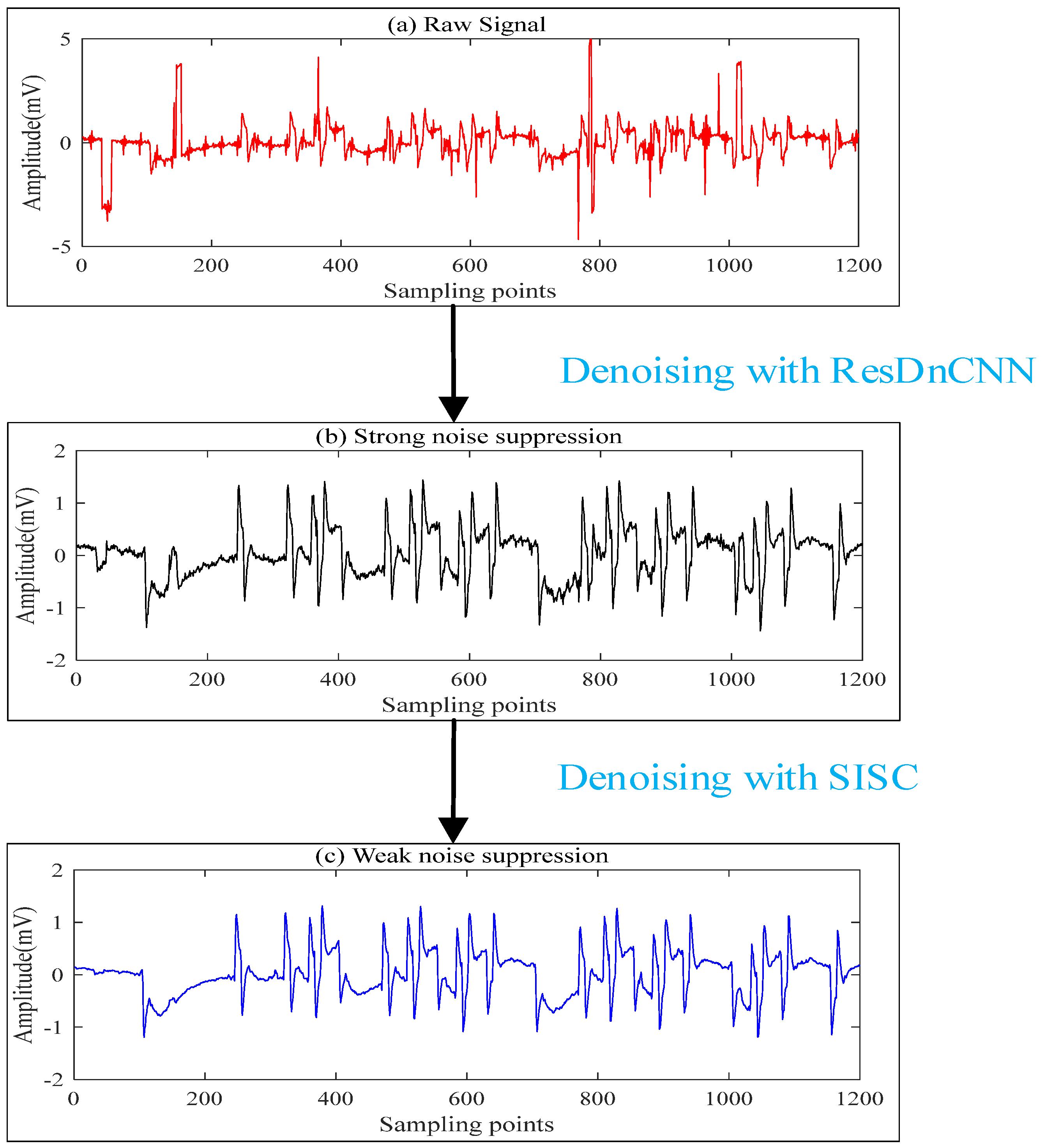
2.1. Overall Experimental Process
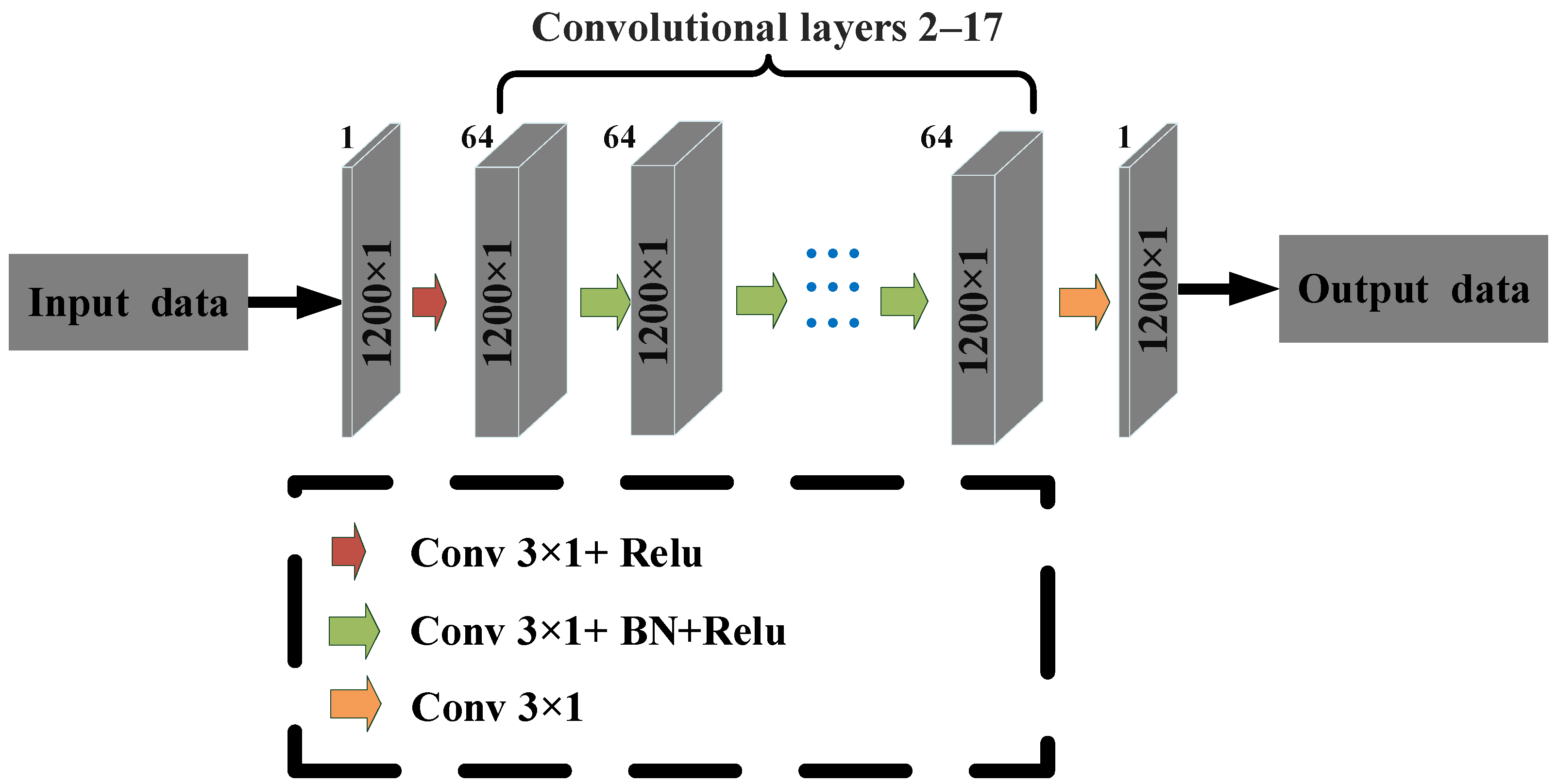
2.2. Denoising Convolutional Neural Network (DnCNN)
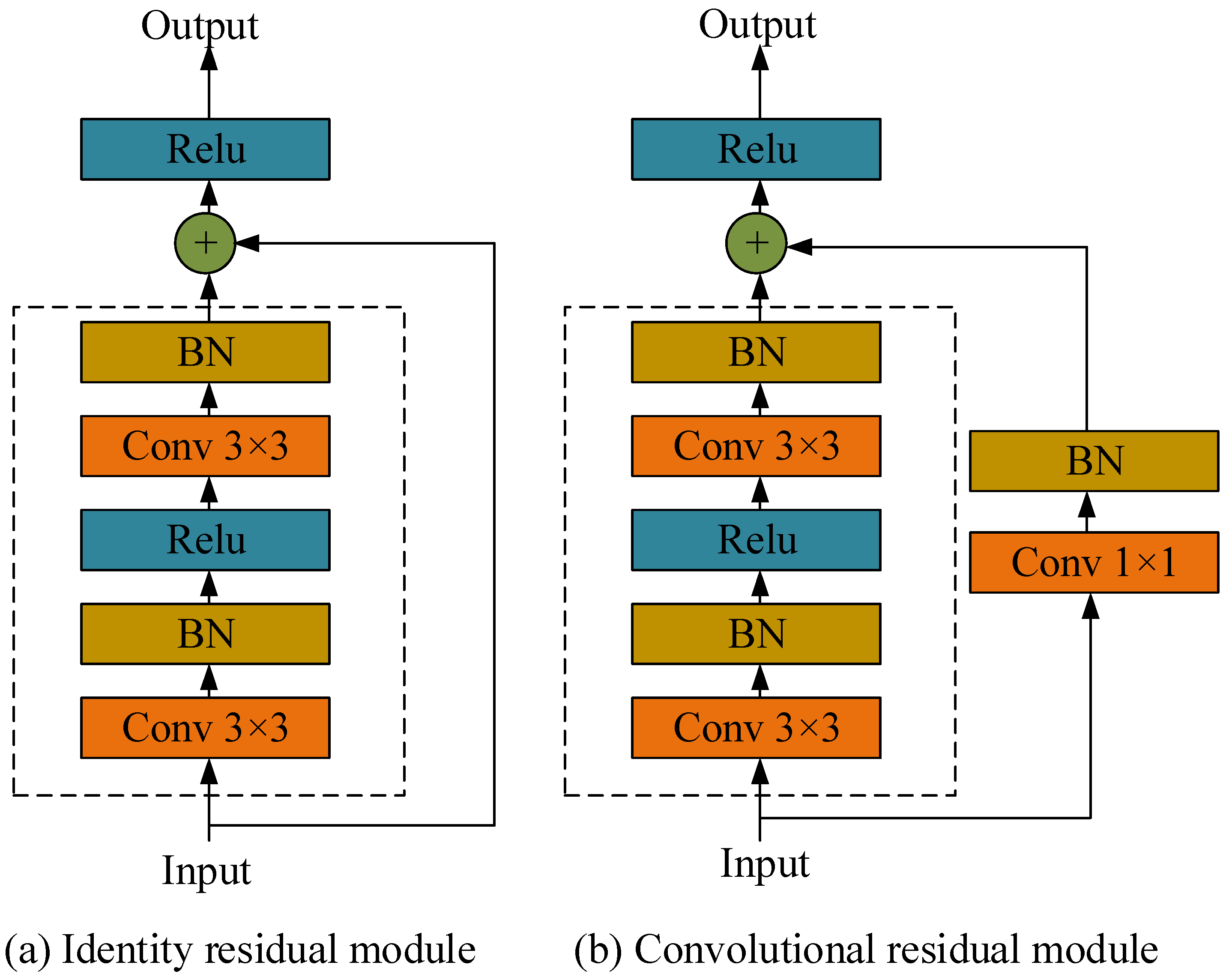
2.3. Residual Network (ResNet)
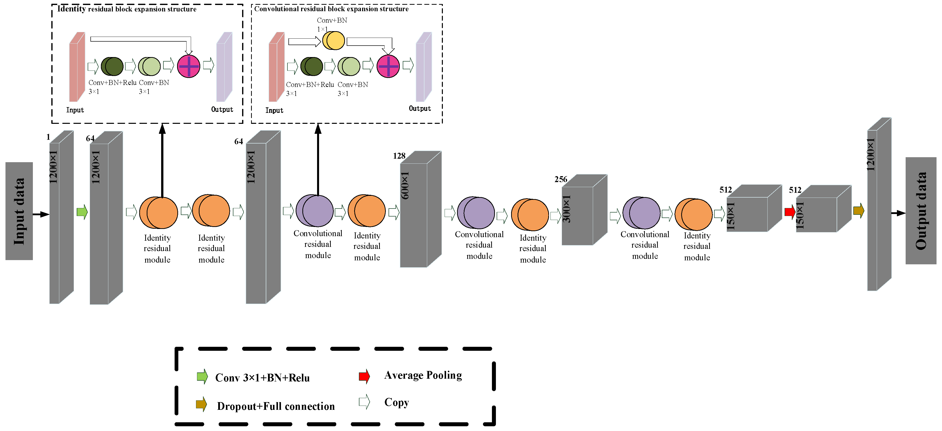
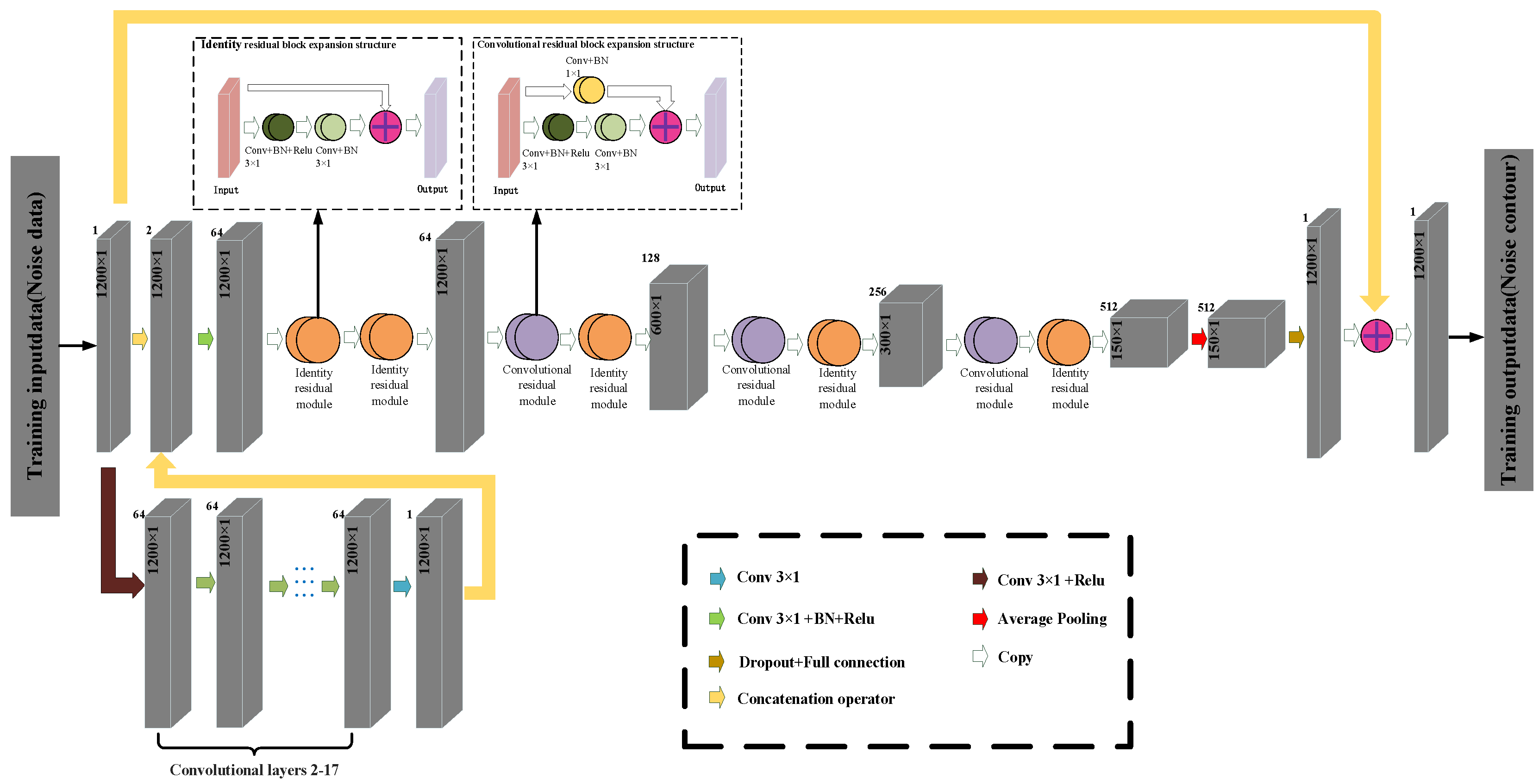
2.4. Residual Denoising Convolutional Neural Network (ResDnCNN)
2.5. The Wide-Field Electromagnetic Method
3. Production of Sample Library and Model Training
3.1. Production of Sample Library
3.2. Model Training
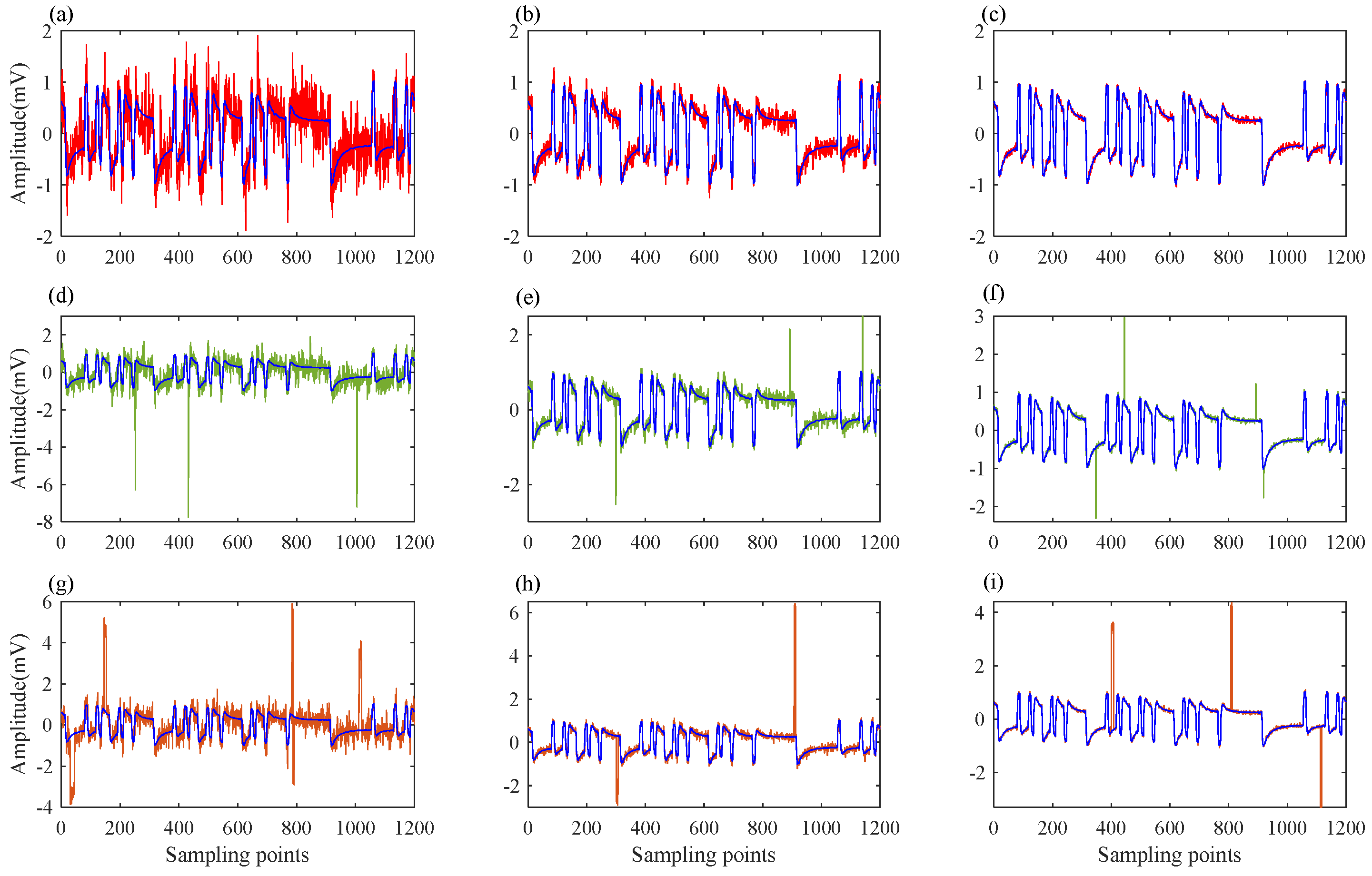
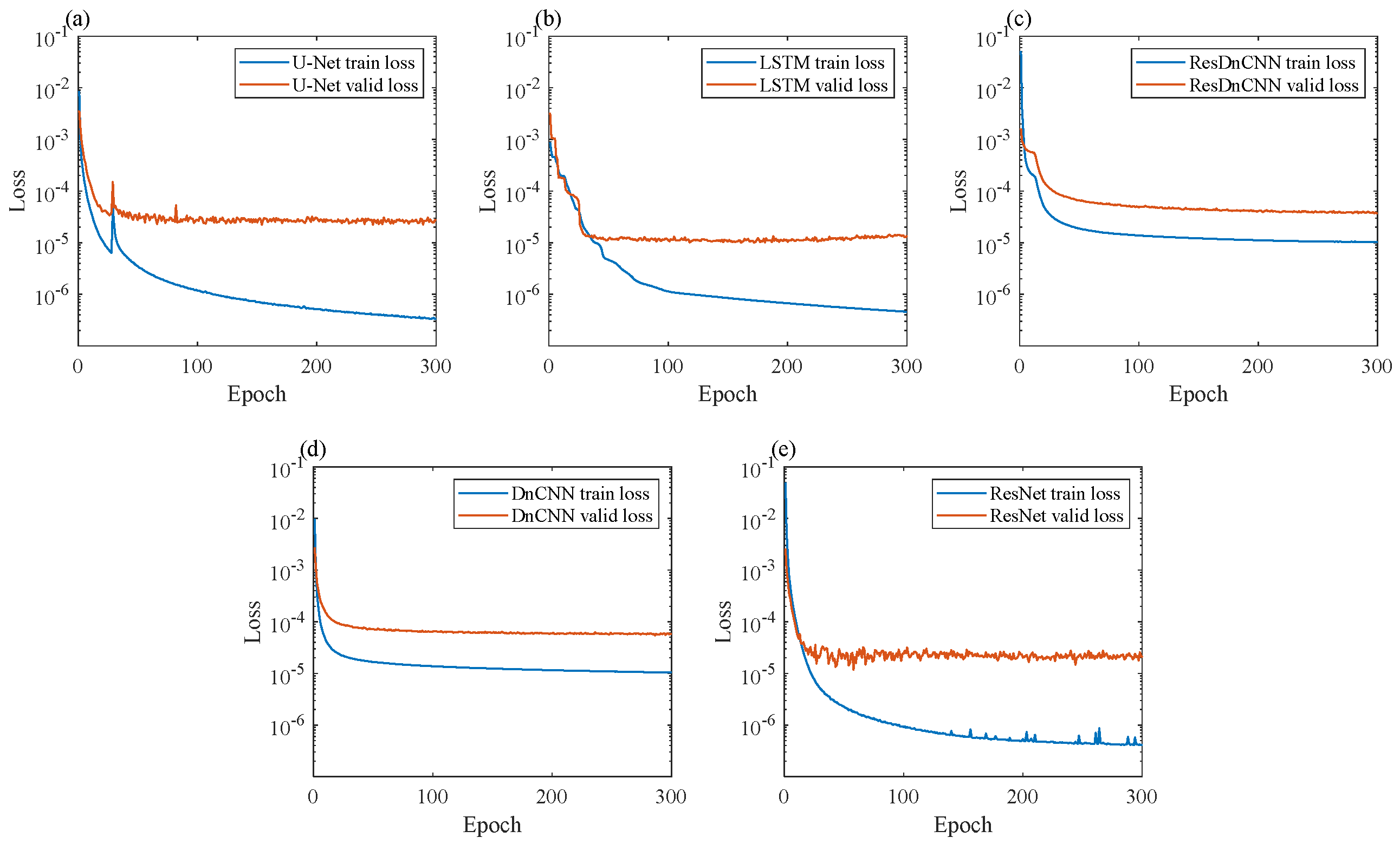
3.3. Denoising Resulte of the Validation Set
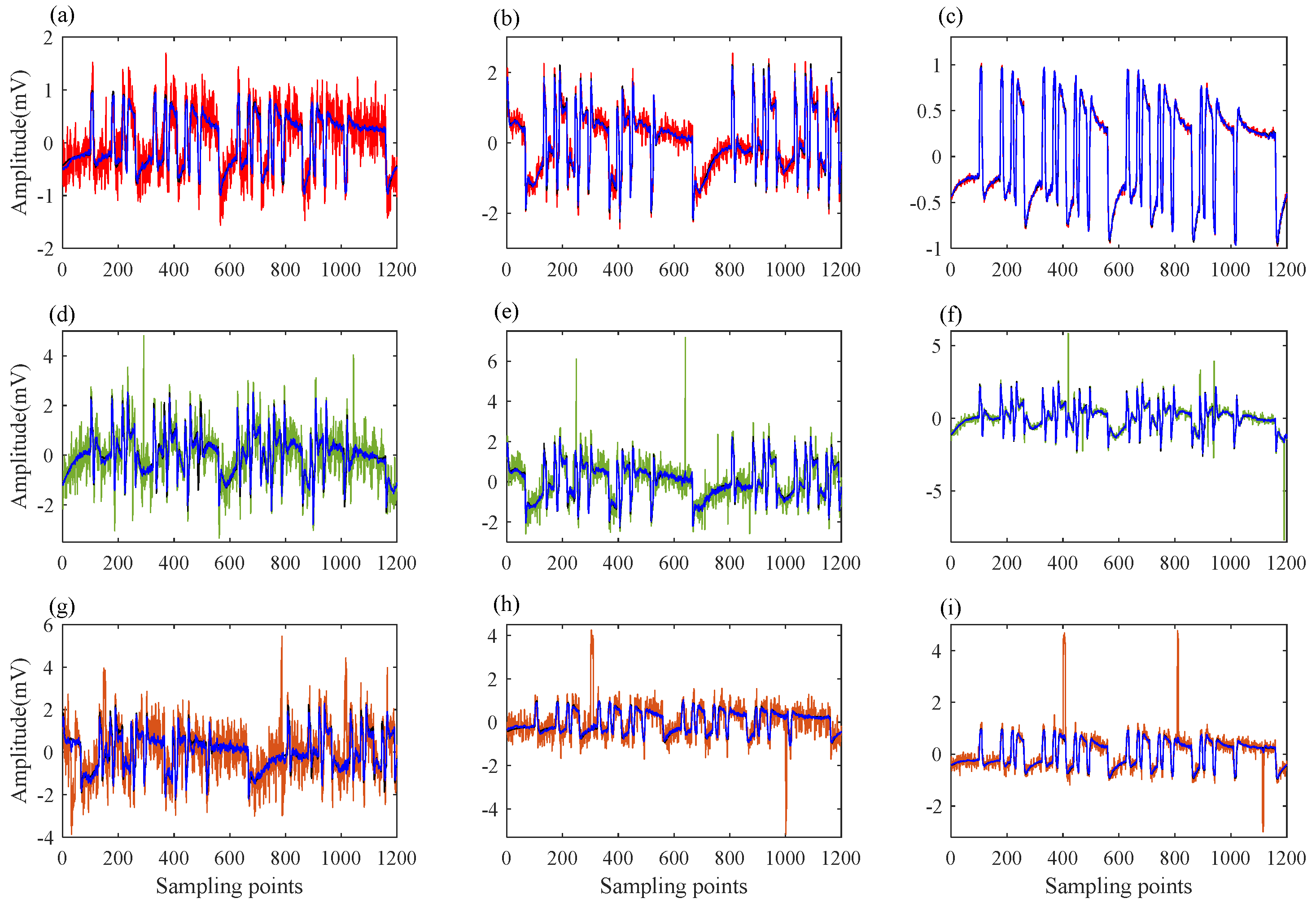
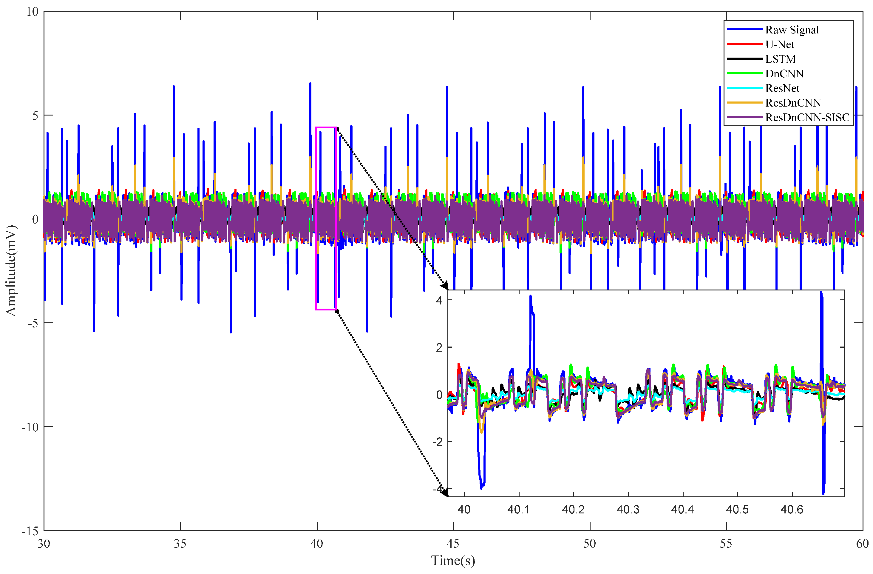
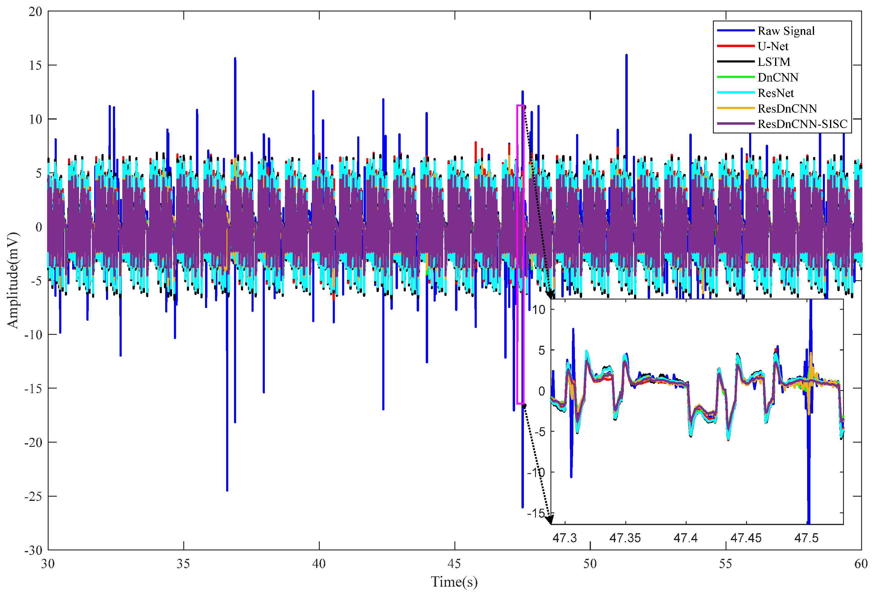
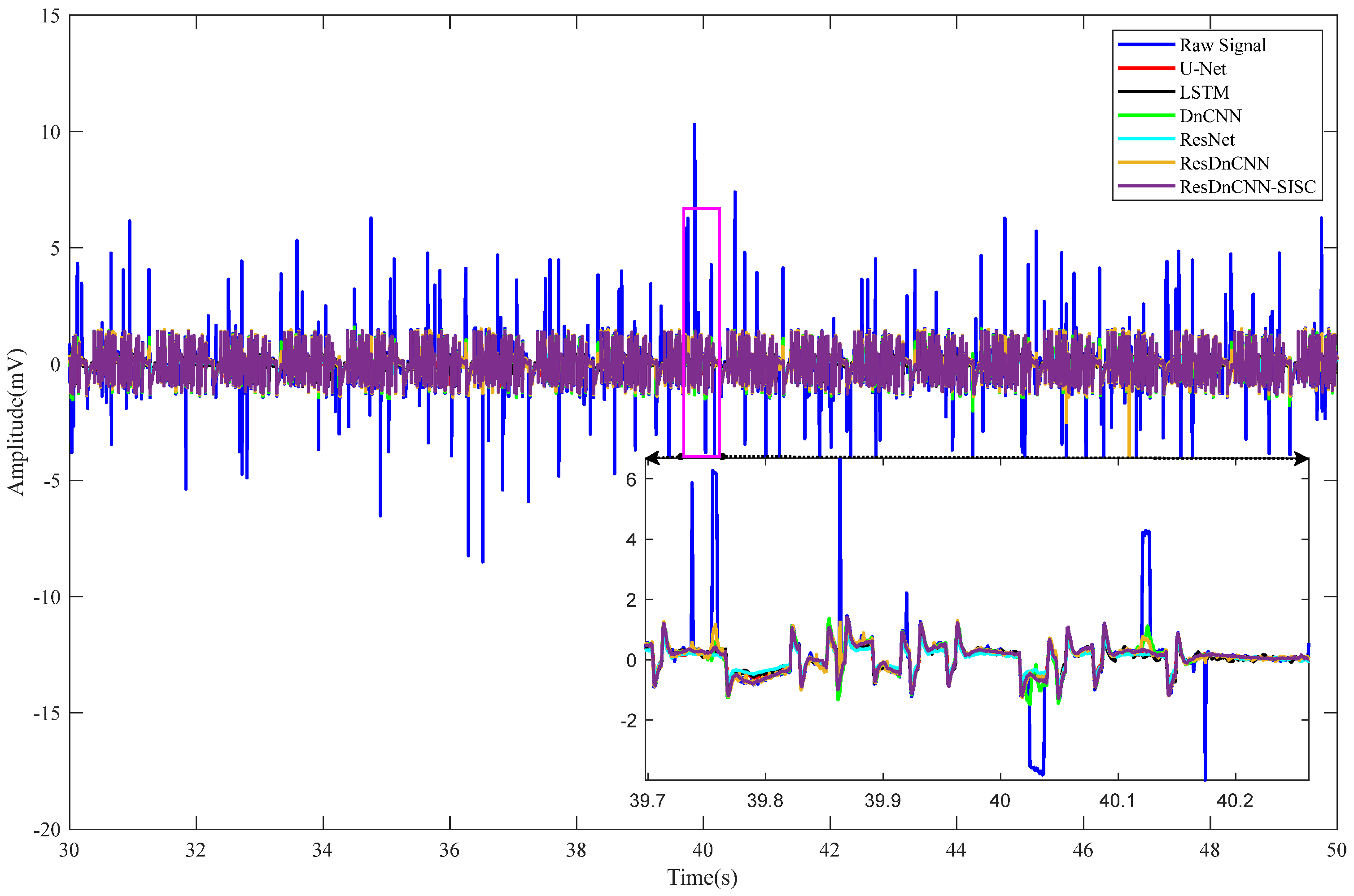
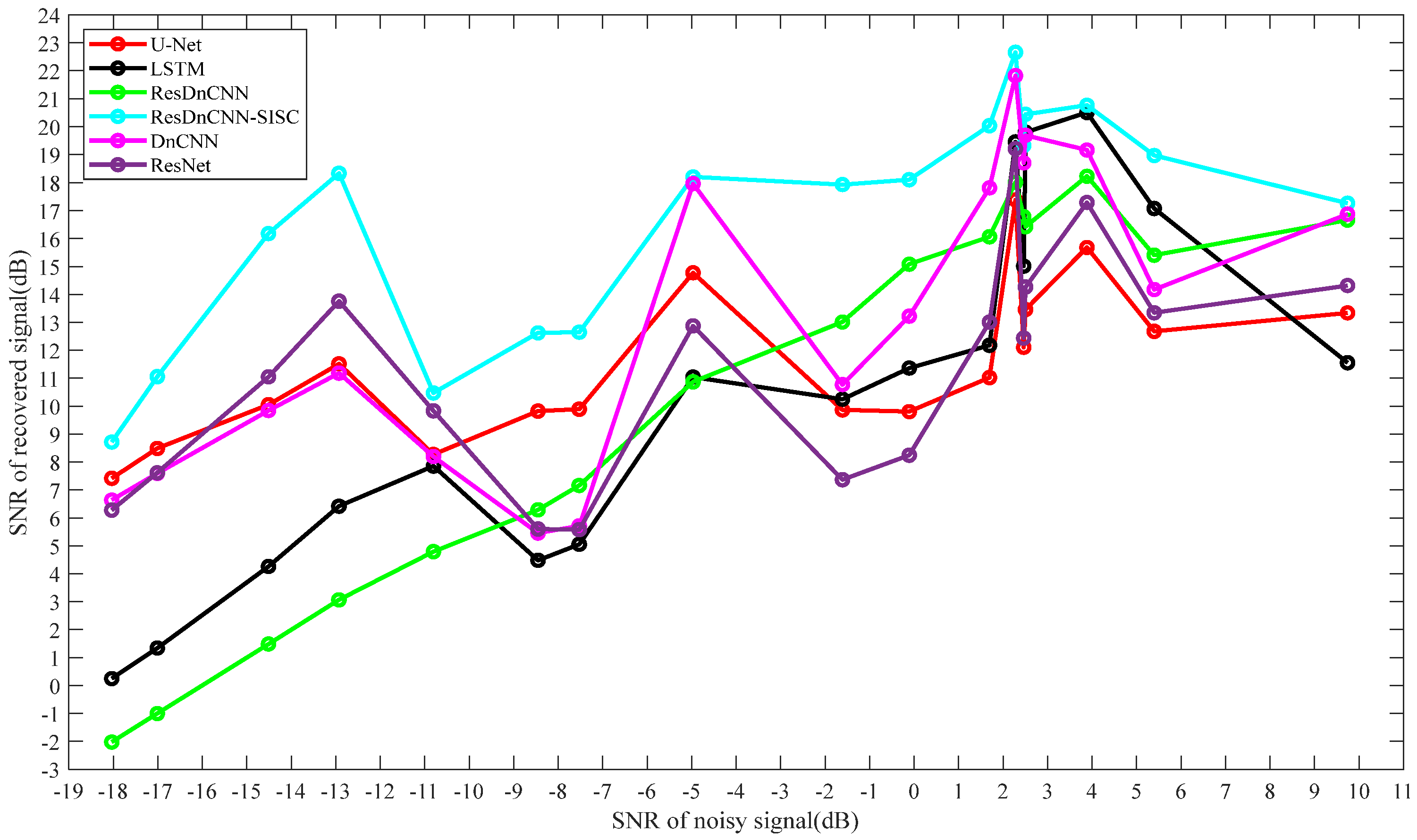
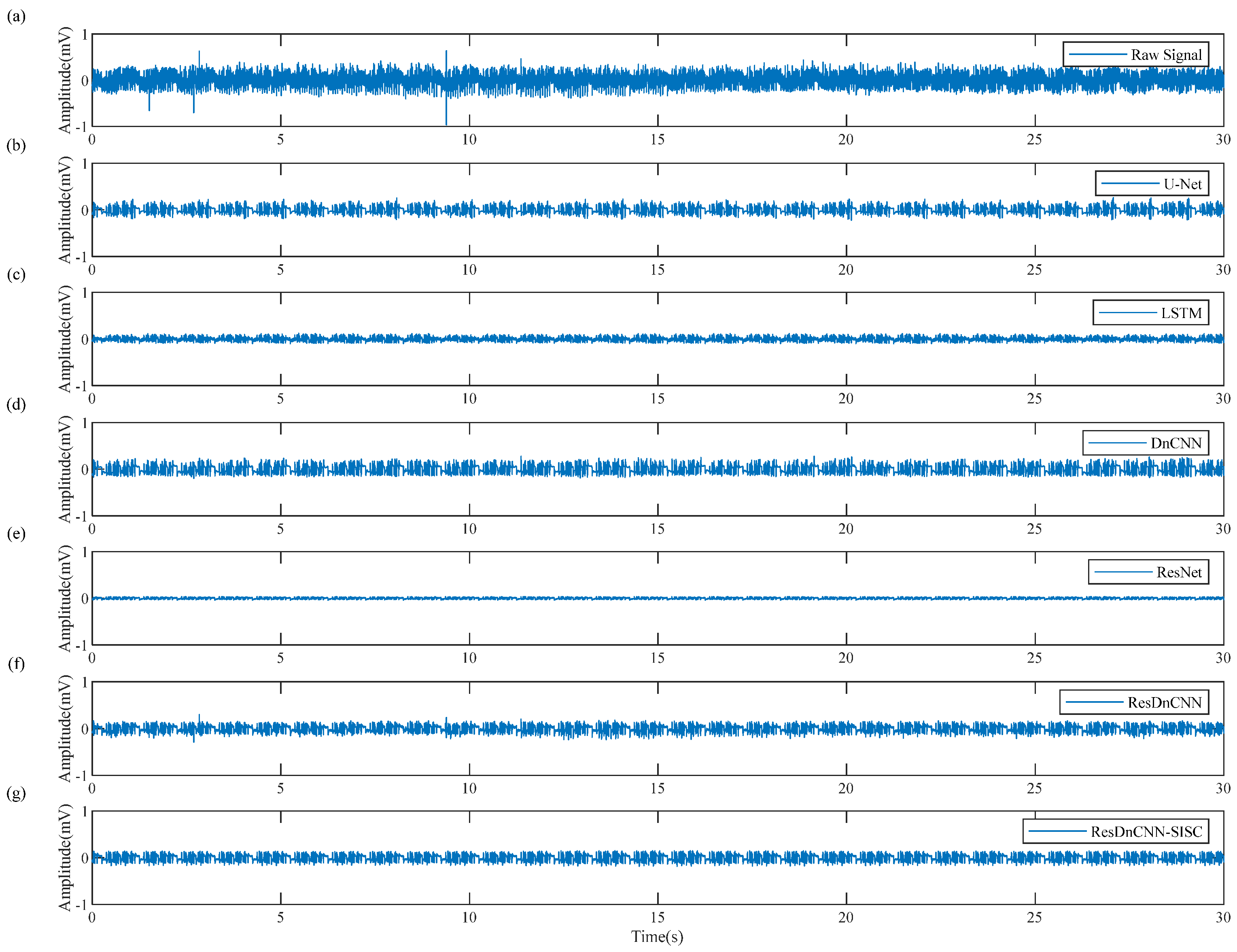
4. Synthetic Data
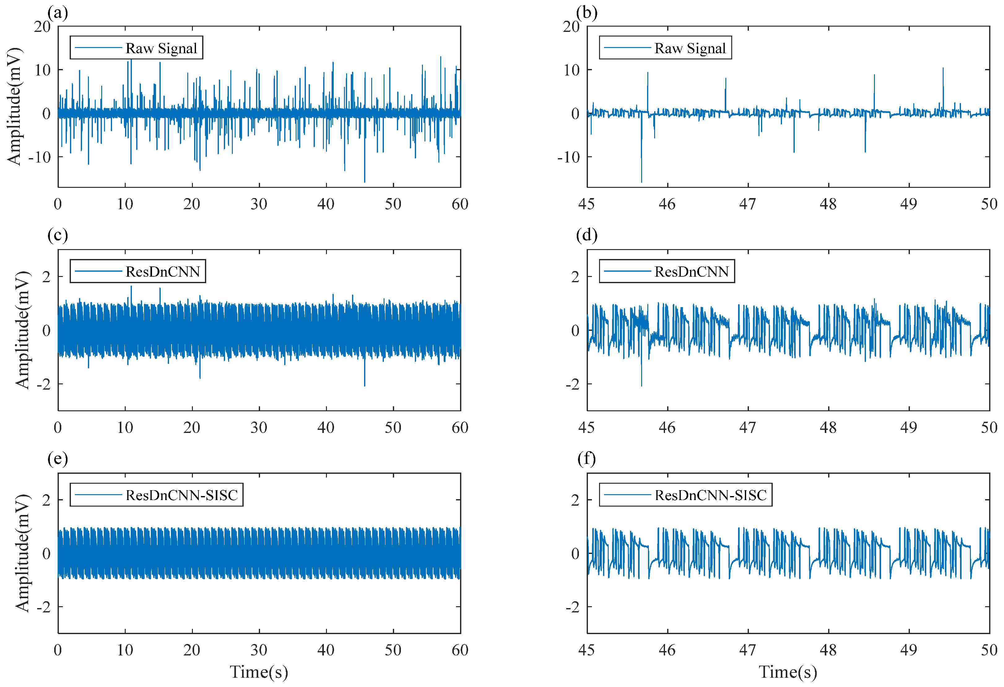
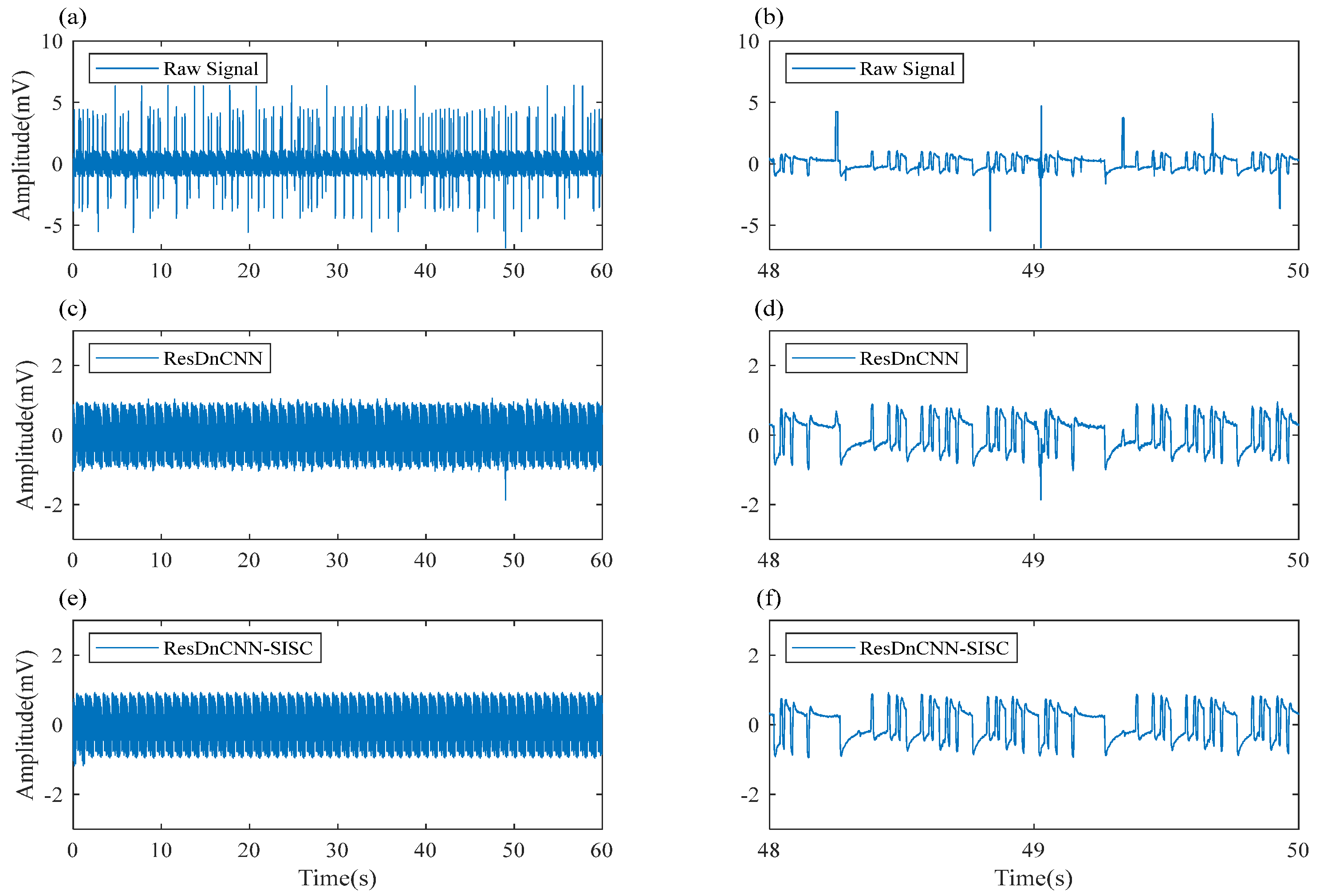
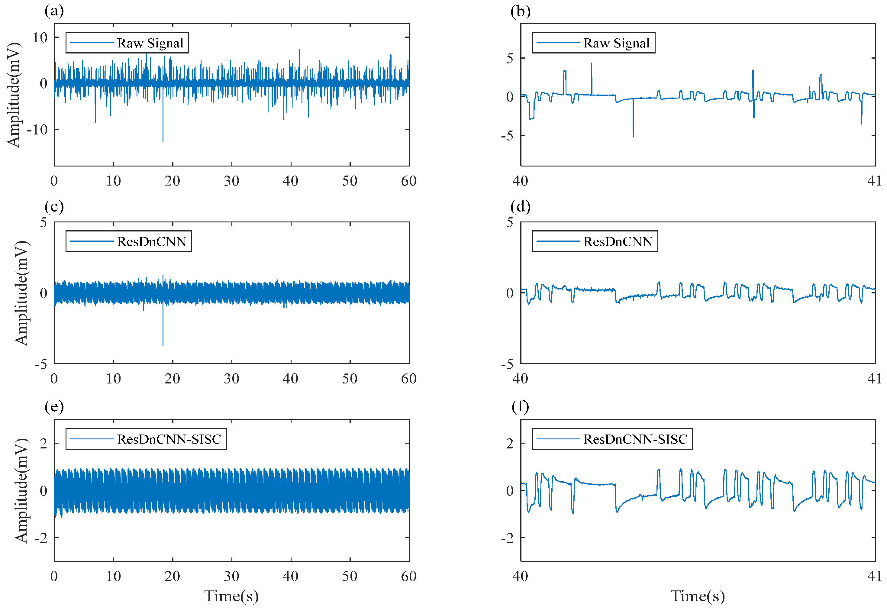
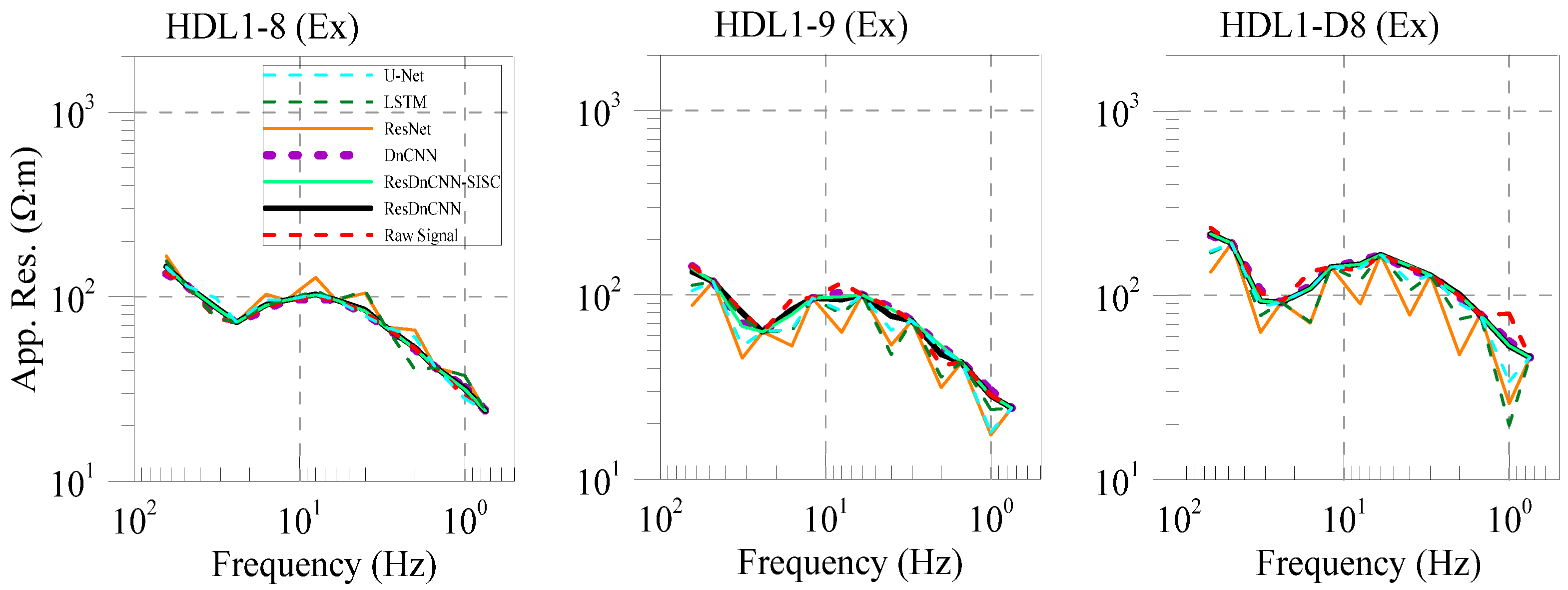
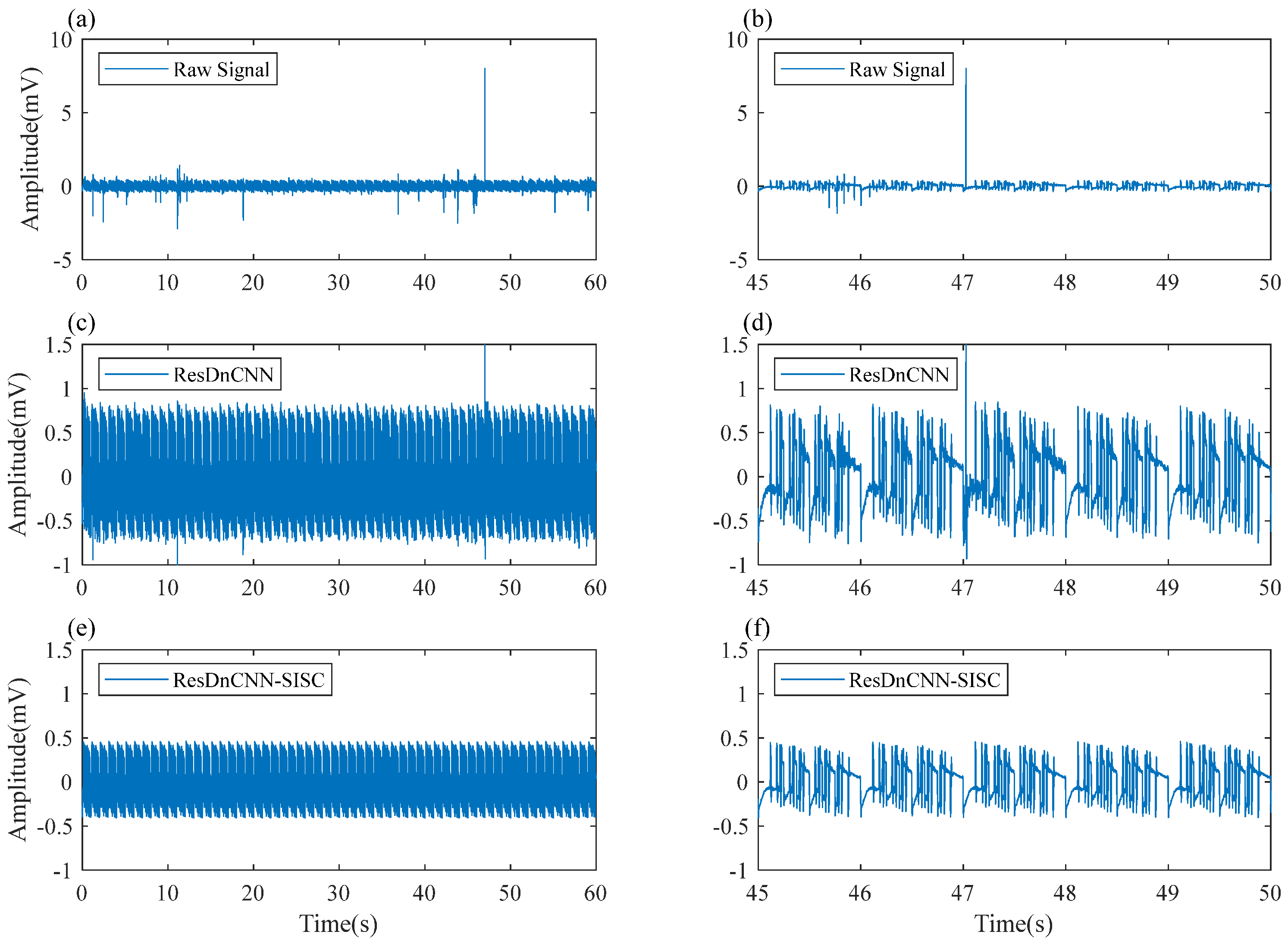
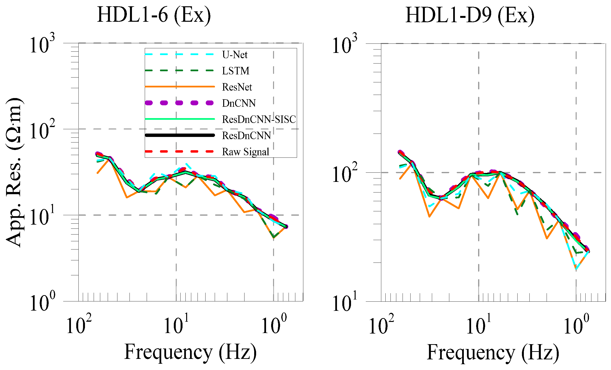
5. Measured Data
6. Conclusions
Author Contributions
Funding
Data Availability Statement
Acknowledgments
Conflicts of Interest
References
- Cai, H.Z.; Long, Z.D.; Lin, W.; Li, J.H.; Lin, P.R.; Hu, X.Y. 3D multinary inversion of controlled-source electromagnetic data based on the finite-element method with unstructured mesh. Geophysics 2021, 86, E77–E92. [Google Scholar] [CrossRef]
- Liu, Y.J.; Yogeshwar, P.; Hu, X.Y.; Peng, R.H.; Tezkan, B.; Morbe, W.; Li, J.H. Effects of electrical anisotropy on long-offset transient electromagnetic data. Geophys. J. Int. 2020, 222, 1074–1089. [Google Scholar] [CrossRef]
- Johansen, S.E.; Panzner, M.; Mittet, R.; Amundsen, H.E.F.; Lim, A.; Vik, E.; Landro, M.; Arntsen, B. Deep electrical imaging of the ultraslow-spreading Mohns Ridge. Nature 2019, 567, 379–383. [Google Scholar] [CrossRef] [PubMed]
- Danielsen, J.E.; Auken, E.; Jørgensen, F.; Søndergaard, V.; Sørensena, K.L. The application of the transient electromagnetic method in hydrogeophysical surveys. J. Appl. Geophys. 2003, 53, 181–198. [Google Scholar] [CrossRef]
- Myer, D.; Constable, S.; Key, K. Broad-band waveforms and robust processing for marine CSEM surveys. Geophys. J. Int. 2011, 184, 698. [Google Scholar] [CrossRef]
- Finn, C.A.; Bedrosian, P.A.; Holbrook, W.S.; Auken, E.; Bloss, B.R.; Crosbie, J. Geophysical Imaging of the Yellowstone’s Hydrothermal Plumbing System. Nature 2022, 603, 643–651. [Google Scholar] [CrossRef]
- Maclennan, K.; Li, Y.G. Denoising multicomponent CSEM data with equivalent source processing techniques. Geophysics 2013, 78, E125–E135. [Google Scholar] [CrossRef]
- Cao, M.; Tan, H.D.; Wang, K.P. 3D LBFGS inversion of controlled source extremely low frequency electromagnetic data. Appl. Geophys. 2017, 13, 689–700. [Google Scholar] [CrossRef]
- Grayver, A.V.; Streich, R.; Ritter, O. 3D inversion and resolution analysis of land-based CSEM data from the Ketzin CO2 storage formation. Geophysics 2014, 79, E101–E114. [Google Scholar] [CrossRef]
- Streich, R.; Becken, M.; Ritter, O. Robust processing of noisy land-based controlled-source electromagnetic data. Geophysics 2013, 78, E237–E247. [Google Scholar] [CrossRef]
- Constable, S.; Srnka, L.J. An introduction to marine controlled-source electromagnetic methods for hydrocarbon exploration. Geophysics 2007, 72, WA3–WA12. [Google Scholar] [CrossRef]
- He, J.S. Combined Application of Wide-Field Electromagnetic Method and Flow Field Fitting Method for High-Resolution Exploration: A Case Study of the Anjialing No. 1 Coal Mine. Engineering 2018, 4, 667–675. [Google Scholar] [CrossRef]
- Reninger, P.A.; Martelet, G.; Deparis, J.; Perrin, J.; Chen, Y. Singular value decomposition as a denoising tool for airborne time domain electromagnetic data. J. Appl. Geophys. 2011, 75, 264–276. [Google Scholar] [CrossRef]
- Rasmussen, S.; Nyboe, N.S.; Mai, S.; Larsen, J.J. Extraction and use of noise models from transient electromagnetic data. Geophysics 2018, 83, E37–E46. [Google Scholar] [CrossRef]
- Yang, Y.; Li, D.Q.; Tong, T.G.; Zhang, D.; Zhou, Y.T.; Chen, Y.K. Denoising controlled-source electromagnetic data using least-squares inversion. Geophysics 2018, 83, E229–E244. [Google Scholar] [CrossRef]
- Barfod, A.S.; Levy, L.; Larsen, J.J. Automatic Processing of Time Domain Induced Polarization Data using Supervised Artificial Neural Networks. Geophys. J. Int. 2011, 224, 312–325. [Google Scholar] [CrossRef]
- Li, G.; Wu, S.L.; Cai, H.Z.; He, Z.S.; Liu, X.Q.; Zhou, C.; Tang, J.T. IncepTCN: A new deep temporal convolutional network combined with dictionary learning for strong cultural noise elimination of controlled-source electromagnetic data. Geophysics 2023, 88, E107–E122. [Google Scholar] [CrossRef]
- Yang, Z.; Tang, J.T.; Xiao, X.; Jiang, Q.Y.; Huang, X.Y.; Hu, S.G. Application of powerline noise cancellation method in correlation identification of controlled source electromagnetic method. J. Geophys. Eng. 2021, 18, 339–354. [Google Scholar] [CrossRef]
- Liu, W.Q.; Chen, R.J.; Cai, H.Z.; Luo, W.B.; Revil, A. Correlation analysis for spread-spectrum induced-polarization signal processing in electromagnetically noisy environments. Geophysics 2017, 82, E243–E256. [Google Scholar] [CrossRef]
- Liu, W.Q.; Lu, Q.T.; Chen, R.J.; Lin, P.R.; Chen, C.J.; Yang, L.Y.; Cai, H.Z. A modified empirical mode decomposition method for multiperiod time-series detrending and the application in full-waveform induced polarization data. Geophys. J. Int. 2019, 217, 1058–1079. [Google Scholar] [CrossRef]
- Zhang, P.F.; Pan, X.P.; Guo, Z.W.; Liu, J.X.; Hou, Q.Y. Marine controlled-source electromagnetic data denoising while weak signal preserving based on jointly sparse model and dictionary learning. J. Appl. Geophys. 2023, 215, 105122. [Google Scholar] [CrossRef]
- Xue, S.Y.; Yin, C.C.; Su, Y.; Liu, Y.H.; Wang, Y.; Liu, C.H.; Xiong, B.; Sun, H.F. Airborne electromagnetic data denoising based on dictionary learning. Appl. Geophys. 2020, 17, 306–313. [Google Scholar] [CrossRef]
- Li, G.; He, Z.S.; Tang, J.T.; Deng, J.Z.; Liu, X.Q.; Zhu, H.J. Dictionary learning and shift-invariant sparse coding denoising for controlled-source electromagnetic data combined with complementary ensemble empirical mode decomposition. Geophysics 2021, 86, E185–E198. [Google Scholar] [CrossRef]
- He, S.Y.; Cai, H.Z.; Liu, S.; Xie, J.T.; Hu, X.Y. Recovering 3D Basement Relief Using Gravity Data Through Convolutional Neural Networks. J. Geophys. Res.-Solid Earth 2021, 126, e2021JB022611. [Google Scholar] [CrossRef]
- Jifara, W.; Jiang, F.; Rho, S.; Chen, M.W.; Liu, S.H. Medical image denoising using convolutional neural network: A residual learning approach. J. Supercomput. 2019, 75, 704–718. [Google Scholar] [CrossRef]
- Pan, X.; Zhao, J.; Xu, J. A Scene Images Diversity Improvement Generative Adversarial Network for Remote Sensing Image Scene Classification. IEEE Geosci. Remote Sens. Lett. 2020, 17, 1692–1696. [Google Scholar] [CrossRef]
- Grais, E.M.; Plumbley, M.D. Single channel audio source separation using convolutional denoising autoencoders. In Proceedings of the IEEE Global Conference on Signal and Information Processing, Montreal, QC, Canada, 14–16 November 2017; pp. 1265–1269. [Google Scholar]
- Wu, X.; Xue, G.Q.; Xiao, P.; Li, J.T.; Liu, L.H.; Fang, G.Y. The Removal of The High-Frequency Motion-Induced Noise in Helicopter-Borne Transient Electromagnetic Data Based on Wavelet Neural Network. Geophysics 2019, 84, K1–K9. [Google Scholar] [CrossRef]
- Lin, F.Q.; Chen, K.C.; Wang, X.B.; Cao, H.; Chen, D.L.; Chen, F.Z. Denoising stacked autoencoders for transient electromagnetic signal denoising. Nonlinear Proc. Geoph. 2019, 26, 13–23. [Google Scholar] [CrossRef]
- Wu, S.H.; Huang, Q.H.; Zhao, L. De-noising of transient electromagnetic data based on the long short-term memory-autoencoder. Geophys. J. Int. 2021, 224, 669–681. [Google Scholar] [CrossRef]
- Li, J.F.; Liu, Y.H.; Yin, C.C.; Ren, X.Y.; Su, Y. Fast imaging of time-domain airborne EM data using deep learning technology. Geophysics 2020, 85, E163–E170. [Google Scholar] [CrossRef]
- Bang, M.; Oh, S.; Noh, K.; Seol, S.J.; Byun, J. Imaging subsurface orebodies with airborne electromagnetic data using a recurrent neural network. Geophysics 2021, 86, E407–E419. [Google Scholar] [CrossRef]
- Sun, Y.S.; Huang, S.H.; Zhang, Y.; Lin, J. Denoising of Transient Electromagnetic Data Based on the Minimum Noise Fraction-Deep Neural Network. IEEE Geosci. Remote Sens. Lett. 2022, 19, 8028405. [Google Scholar] [CrossRef]
- Zhang, K.; Zuo, W.M.; Chen, Y.J.; Meng, D.Y.; Zhang, L. Beyond a gaussian denoiser: Residual Learning of deep cnn for image denoising. IEEE Trans. Image Process. 2017, 26, 3142–3155. [Google Scholar] [CrossRef]
- He, K.M.; Zhang, X.Y.; Ren, S.Y.; Sun, J. Deep Residual Learning for Image Recognition. In Proceedings of the IEEE Conference on Computer Vision and Pattern Recognition, Las Vegas, NV, USA, 27–30 June 2016; pp. 770–778. [Google Scholar]
- Dong, X.T.; Li, Y.; Yang, B.J. Desert low-frequency noise suppression by using adaptive DnCNNs based on the determination of high-order statistic. Geophys. J. Int. 2019, 219, 1281–1299. [Google Scholar] [CrossRef]
- Li, G.; Zhou, X.; Chen, C.; Xu, L.; Zhou, F.; Shi, F.; Tang, J. Multi-type geomagnetic noise removal via an improved U-Net deep learning network. IEEE Trans. Geosci. Remote Sens. 2023, 61, 3307422. [Google Scholar] [CrossRef]
- Li, Z.; Zhu, Y.P.; Wang, Y.P. A Criminisi-DnCNN Model-Based Image Inpainting Method. Math. Probl. Eng. 2022, 2022, 9780668. [Google Scholar] [CrossRef]
- Wei, F.; Zhu, Z.H.; Zhou, H.; Tao, Z.; Jun, S.; Wu, X.J. Efficient automatically evolving convolutional neural network for image denoising. Memet. Comput. 2022, 15, 219–235. [Google Scholar] [CrossRef]
- Karthikeyan, V.; Raja, E.; Pradeep, D. Energy based denoising convolutional neural network for image enhancement. Imaging Sci. J. 2023, volume, 1–16. [Google Scholar] [CrossRef]
- Yuan, Y.J.; Zheng, Y.; Si, X. Attenuation of linear noise based on denoising convolutional neural network with asymmetric convolution blocks. Explor. Geophys. 2022, 53, 532–546. [Google Scholar] [CrossRef]
- Dong, X.T.; Lin, J.; Lu, S.P.; Wang, H.Z.; Li, Y. Multiscale Spatial Attention Network for Seismic Data Denoising. IEEE Trans. Geosci. Remote Sens. 2022, 60, 1–17. [Google Scholar] [CrossRef]
- Feng, X.B.; Zhang, W.X.; Su, X.Q.; Xu, Z.P. Optical Remote Sensing Image Denoising and Super-Resolution Reconstructing Using Optimized Generative Network in Wavelet Transform Domain. Remote Sens. 2021, 13, 1858. [Google Scholar] [CrossRef]
- Duan, R.F.; Chen, Z.Y.; Zhang, H.T.; Wang, X.; Meng, W.; Sun, G.D. Dual Residual Denoising Autoencoder with Channel Attention Mechanism for Modulation of Signals. Sensors 2023, 23, 1023. [Google Scholar] [CrossRef] [PubMed]


| Method | SNR (dB) | Reconstruction Error | NCC |
|---|---|---|---|
| Noisy | −2.9118 | 1.39% | 0.5828 |
| U-Net | 9.9061 | 0.31% | 0.9541 |
| LSTM | 6.4761 | 0.47% | 0.8882 |
| DnCNN | 10.0815 | 0.31% | 0.9526 |
| ResNet | 5.7866 | 0.51% | 0.9520 |
| ResDnCNN | 10.2678 | 0.30% | 0.9520 |
| ResDnCNN-SISC | 14.2147 | 0.19% | 0.9848 |
Disclaimer/Publisher’s Note: The statements, opinions and data contained in all publications are solely those of the individual author(s) and contributor(s) and not of MDPI and/or the editor(s). MDPI and/or the editor(s) disclaim responsibility for any injury to people or property resulting from any ideas, methods, instructions or products referred to in the content. |
© 2023 by the authors. Licensee MDPI, Basel, Switzerland. This article is an open access article distributed under the terms and conditions of the Creative Commons Attribution (CC BY) license (https://creativecommons.org/licenses/by/4.0/).
Share and Cite
Wang, X.; Bai, X.; Li, G.; Sun, L.; Ye, H.; Tong, T. Noise Attenuation for CSEM Data via Deep Residual Denoising Convolutional Neural Network and Shift-Invariant Sparse Coding. Remote Sens. 2023, 15, 4456. https://doi.org/10.3390/rs15184456
Wang X, Bai X, Li G, Sun L, Ye H, Tong T. Noise Attenuation for CSEM Data via Deep Residual Denoising Convolutional Neural Network and Shift-Invariant Sparse Coding. Remote Sensing. 2023; 15(18):4456. https://doi.org/10.3390/rs15184456
Chicago/Turabian StyleWang, Xin, Ximin Bai, Guang Li, Liwei Sun, Hailong Ye, and Tao Tong. 2023. "Noise Attenuation for CSEM Data via Deep Residual Denoising Convolutional Neural Network and Shift-Invariant Sparse Coding" Remote Sensing 15, no. 18: 4456. https://doi.org/10.3390/rs15184456