Article

Polar Cap Patches Scaling Properties: Insights from Swarm Data

1
Istituto Nazionale di Geofisica e Vulcanologia, Via di Vigna Murata 605, 00143 Rome, Italy
2
Dipartimento di Fisica, Università di Roma Sapienza, 00185 Rome, Italy
3
INAF-Istituto di Astrofisica e Planetologia Spaziali, Via del Fosso del Cavaliere 100, 00133 Rome, Italy
*
Author to whom correspondence should be addressed.
Remote Sens. 2023, 15(17), 4320; https://doi.org/10.3390/rs15174320
Submission received: 25 July 2023 / Revised: 18 August 2023 / Accepted: 20 August 2023 / Published: 1 September 2023

Abstract

:
Among the effects of space weather, the degradation of air traffic communications and satellite-based navigation systems are the most notable. For this reason, it is of uttermost importance to understand the nature and origin of ionospheric irregularities that are at the base of the observed communication outages. Here we focus on polar cap patches (PCPs) that constitute a special class of ionospheric irregularities observed at very high latitudes in the F region. To this purpose we use the so-called PCP flag, a Swarm Level 2 product, that allows for identifying PCPs. We relate the presence of PCPs to the values of the first- and second-order scaling exponents and intermittency estimated from Swarm A electron density fluctuations and to the values of the Rate Of change of electron Density Index (RODI) for two different levels of geomagnetic activity, over a time span of approximately 3.5 years starting on 16 July 2014. Our findings show that values of RODI, first- and second-order scaling exponents and intermittency corresponding to measurements taken inside PCPs differ from those corresponding to measurements taken outside PCPs. Additionally, the values of the first- and second-order scaling exponents and of intermittency indicate that PCPs are in a turbulent state. Investigation of the coincidence of loss of lock (LoL) events with PCPs displayed that approximately 57.4% of LoLs in the Northern hemisphere and 45.7% in the Southern hemisphere occur in coincidence of PCPs when disturbed geomagnetic activity is considered. During quiet geomagnetic conditions these percentages decrease to 51.4% in the Northern hemisphere and to 20.1% in the Southern hemisphere.

Graphical Abstract

1. Introduction

Today, a very large number and variety of human activities depend on precise positioning achievable through Global Navigation Satellite Systems (GNSS) like Galileo, Global Positioning System (GPS), and Global’naja Navigacionnaja Sputnikovaja Sistema (GLONASS). Electromagnetic signals used by this kind of systems travel through the ionosphere whose features, however, can significantly vary both in time and space. Plasma density structuring entails the rise of electron density irregularities and hence the variation in the electromagnetic properties of the ionosphere. Ionospheric irregularities, in particular, can cause interference and diffraction of electromagnetic signals traveling through them, resulting in scintillations [1]. A scintillation causes a degradation of the signal, that may reduce significantly the positioning accuracy, and also trigger a loss of lock (LoL) between the receiver (either on the ground or in situ) and the GNSS satellite. The very low (i.e., equatorial region) and very high latitudes are those that are most susceptible to ionospheric irregularities (e.g., [2,3,4]). In this article, we will focus on the so-called polar cap patches (PCPs), which are one of the many irregularities seen at high latitudes. A PCP can be thought of as an island of plasma whose density is at least double than that of the surrounding background plasma and whose size is approximately in the range 100 ÷ 1000 km. A PCP usually enters the polar cap through the dayside then, driven by ionospheric convection, crosses the polar cap, to finally exiting the polar cap hours later, near midnight [5]. PCPs form from the high-density plasma reservoir found in the dayside ionosphere, where the low solar zenith angles and resulting high solar EUV ionization ensure a much higher plasma density than elsewhere. PCP formation is still a debated topic and different mechanisms have been proposed [6]. According to Lockwood and Carlson Jr. [7], for instance, these islands of high density plasma are produced by the bursty nature of dayside reconnection. When the Dungey cycle is ongoing [8], these are transported across the polar cap by ionospheric convection, which acts exactly like a conveyor belt.
This means that plasma density irregularities can travel for hours and over long distances. Their names change depending on where they are observed. They are only referred to as PCPs if they occur within the polar cap; otherwise, they are referred to as auroral blobs [9]. Because different mechanisms may be in charge of their generation and development, it was decided to separate them by giving them different names.
Due to their drifting nature, PCPs are susceptible to the gradient-drift instability (GDI) [1], which can break them down into smaller plasma structures with sizes as small as a few meters. These small ionospheric irregularities are capable of negatively affecting trans-ionospheric radio signals at commonly used frequencies [10].
Since the first PCP observations, several investigations have been conducted, both through case studies based on data from rockets or satellites (e.g., [11,12,13,14] and references therein) and statistical analyses based on data from long-lived satellites such as CHAMP, Dynamics Explorer 2, and Swarm (e.g., [15,16,17]). Among these, the European Space Agency (ESA) Swarm satellite constellation, which was launched in 2013 and is still in orbit, provides the opportunity to analyze new high-quality data in order to better understand PCP properties and dynamics through a product that identifies PCPs. So, we will use this Swarm product and, taking advantage of the studies on the role of turbulence in the formation of ionospheric irregularities at low-latitudes (e.g., [18,19,20] and references therein) and at mid- and high-latitudes [20,21], we will try to understand if turbulence plays a role also in the formation of PCPs. In detail, by estimating the first- and second-order scaling exponents and intermittency of electron density ( N e ) fluctuations, we examine whether N e measurements taken inside PCPs are characterized by values of these quantities that are different from those taken outside PCPs. This is performed for two different levels of geomagnetic activity, i.e., for quiet and disturbed conditions, based on the values of the auroral electrojet (AE) geomagnetic index. We investigate also the possible relation between the occurrence of PCPs and GPS LoL events.
Section 2 is devoted to the description of all data and method used and to a brief characterization of the time and space distributions of PCPs included in the dataset. Section 3 discusses the obtained results, while conclusions are drawn in Section 4.

2. Data and Methods

2.1. Swarm Data

Data used in this paper span approximately 3.5 years; more specifically, we investigate Swarm A observations between 16 July 2014 and 28 February 2018. Swarm A is one of the three satellites constituting the constellation, that was launched by ESA in November 2013 and is still in orbit today [22]. The constellation is designed so that two satellites, Swarm A and C, fly side-by-side at an altitude that was initially 460 km, and one satellite, Swarm B, flies around 50 km above the other two spacecrafts. The three satellites are equipped with identical instruments designed to guarantee high-precision measurements of physical quantities such as magnetic field, electron density, and temperature [23]. The orbital configuration of the constellation, with inclinations of 87.35 for Swarm A and C and of 87.75 for Swarm B, ensures that each polar cap region (Northern and Southern) is crossed once per orbit, making these satellites particularly suitable for investigating phenomena occurring at high latitudes.
The study relies on electron density measurements from Swarm A, on corresponding values of the Rate Of Change of electron Density Index (RODI), on the PCP flag, and on LoL events identified in previous studies through the slant Total Electron Content (sTEC) measurements [24]. Swarm data are freely available at http://swarm-diss.eo.esa.int (accessed on 31 August 2023).

2.1.1. Electron Density Measurements and RODI
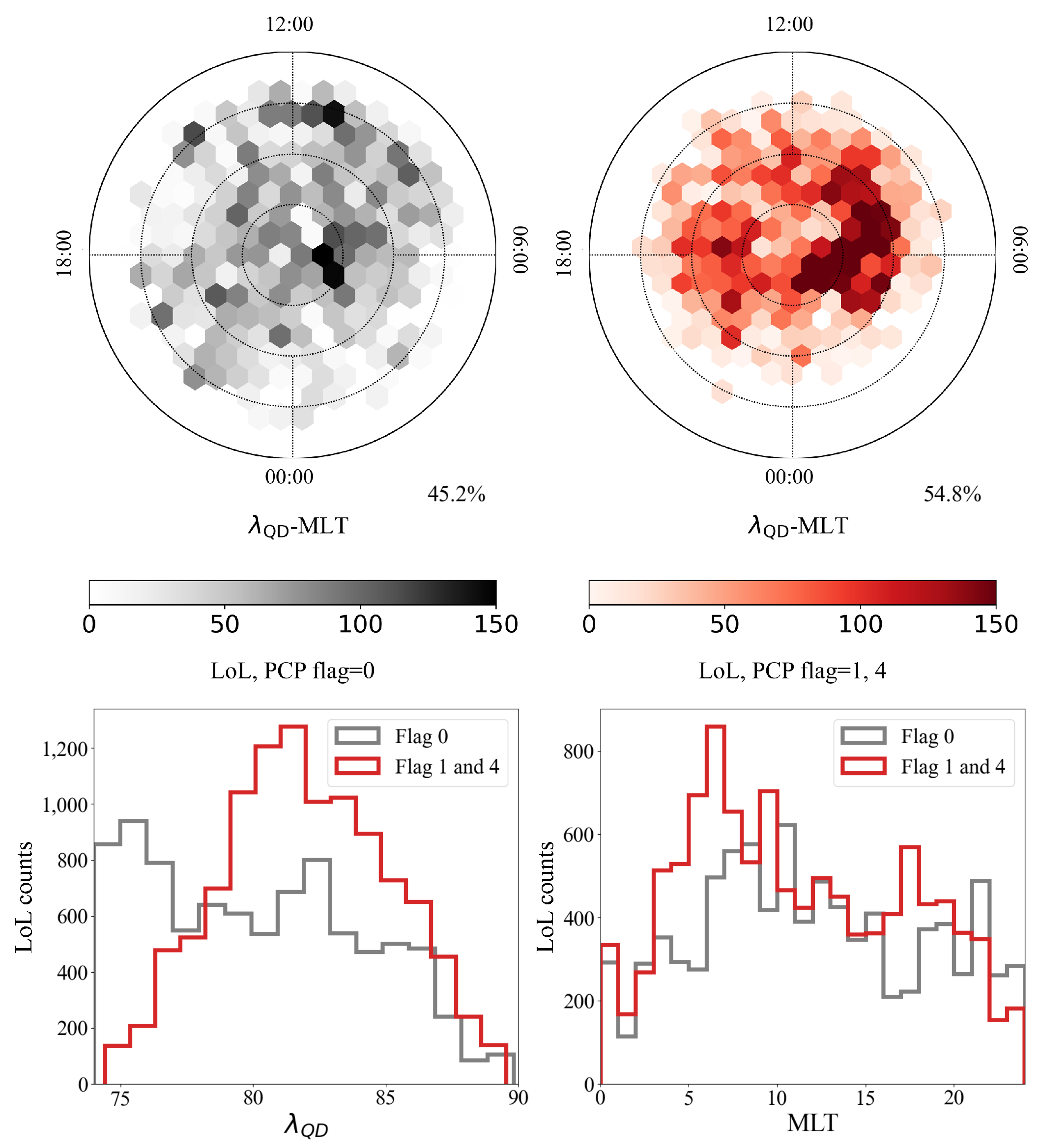
Electron density measurements represent a Swarm Level 1b product. Although they are provided by Langmuir Probes (LP) at a rate of 2 Hz [25,26], we use the 1 Hz dataset distributed through the EFIXLPI_1B product.
RODI, which provides a measure of electron density variability along the satellite track was first used to characterize ionospheric plasma irregularities using data from CHAMP by Zakharenkova and Astafyeva [27] and is now calculated from Swarm satellites and used to investigate a wide range of ionospheric phenomena (see, e.g., [9,24,28,29]). Indeed, because of the way RODI is calculated, it is well suited to study ionospheric irregularities.
RODI is defined as the root mean square error of the first derivative with respect to the time of the electron density, calculated for a specific moving time window (e.g., [24]).
In this work, we calculated RODI values according to the procedure implemented in the tool TITIPy (Topside Ionosphere Turbulence Indices with Python) recently developed by Pignalberi [30], setting the width of the moving time window to 10 s. This allows for investigating irregularities with spatial scales down to ∼70 km.

2.1.2. The PCP Flag

Locating polar cap patches is made possible through the use of the PCP flag, which is contained in the Swarm IPDxIRR Level 2 product [31,32,33]. PCP flag, which is provided at 1 Hz rate, is calculated using 2 Hz electron density observations applying an algorithm developed by Spicher et al. [17] that represents a slightly modified version of that first introduced by Coley and Heelis [34]. Besides that developed by Coley and Heelis [34], other methods have been proposed to identify PCPs, for instance that proposed by Noja et al. [15] or by Chartier et al. [35] who actually proposed a synthesis of previous methods with the purpose to overcome the limits inherent in both Noja et al. [15] and Coley and Heelis [34] algorithms. We are aware of the fact that all of them produce quite different results, especially concerning the spatial and temporal distributions of polar cap patches [35]. However, it is unclear whether discrepancies in results are due to the use of either different types of measurements or detection techniques. In fact, the correct way to identify, or better yet, define this type of irregularity is still debated. All of this, however, is beyond the purpose of this paper, so we decided to rely on the only PCP identification available along the track of Swarm A satellite, which is also distributed as an official ESA Swarm product. In practice, an electron density measurement is flagged to be taken inside a PCP when N e is at least twice the background electron density. One of the main criticisms to this procedure is that even small fluctuations can exceed the doubled value of the background when this is very low. To limit the drawbacks of the algorithm proposed by Coley and Heelis [34], due to the times when low values of the background density are observed, we adopted the strategy proposed by Kagawa et al. [36], i.e., to take only PCPs corresponding to electron density measurements higher than 5 × 10 4 cm 3 . Similarly, an electron density measurement is considered at the border of a PCP when N e measurements adjoining to a PCP are at least 30% the average background density within the PCP [17].
PCP flag is expected to have five values: 0 if the measurement is taken outside of a PCP, 1 if it is taken at the border of a PCP, either 2 or 3 if the border can be identified to be either a leading or trailing edge, respectively, and 4 if it is taken inside a PCP. However, at the present moment, PCP flag only takes three values (0, 1, 4), implying that the nature of the edges of the patches is unknown; so, we only consider N e measurements corresponding to a PCP flag equal to 1 and 4 in order to study processes occurring inside and at the borders of a PCP. So, in the following, PCP borders will be considered as part of the patch. We also want to draw the reader’s attention to the fact that in the distributions that follow, PCPs are counted considering the single N e measurements falling either inside or at the border of PCPs observed in the selected period and not considering as a whole the set of measurements belonging to a PCP. Since values of the PCP flag are available from 16 July 2014 we use this as the start time of our dataset.
The temporal and spatial distribution (for both hemispheres) of the PCP dataset considered in this analysis perfectly matches that found by Spicher et al. [17], even though the time interval considered here is approximately doubled. Indeed, as shown in Figure 1 displaying the time distribution of all PCPs observed in the selected period, the maximum occurrence is observed in the local winter in both hemispheres, with an overall higher number observed in the Northern hemisphere than in the Southern one. As documented in the literature [36,37], the occurrence of PCPs is deeply influenced by the difference in distance between the geographic and magnetic poles in the two hemispheres. This asymmetry reflects both in the total number of PCPs being higher in the Northern hemisphere than in the Southern one and also in the PCPs spatial distribution, as shown in Figure 2, indicating quite a different dependence on quasi-dipole (QD) magnetic latitude and magnetic local time (MLT) between the two hemispheres.
Since we are going to perform a scale analysis, it is crucial to have an idea of the order of magnitude of the spatial extension of PCPs under consideration. An estimate can be obtained by multiplying the temporal length, t , of their observations by the orbital velocity of Swarm A. This is clearly an approximation since it assumes that PCPs are not traveling. Figure 3 displays: in blue, the cumulative distribution function (CDF) and, in red, the probability density function (PDF) of the sizes of the PCPs identified by the Swarm PCP flag. More than 90% out of the 32,382 identified PCPs have a dimension x in the range 50 ÷ 1350 km, as expected. To have an idea of the corresponding error we can consider that Swarm A has a speed of ∼7.6 km/s and PCPs have a maximum speed of ∼1 km/s (i.e., the maximum value for plasma drift in the F-region) [5]. Based on simple kinematic considerations, we expect the maximum error in our estimate of PCP size to be ∼11% when the spacecraft and the PCP move in opposite directions, which is the case with the greatest relative speed between the satellite and the PCP. Since we are assuming that PCP size is proportional to the time needed by the satellite to cross the patch, the error made in case of a patch that is not fixed in space can be estimated by the ratio of the relative speed between the spacecraft and the patch to the speed of the spacecraft. In practice, this ratio corresponds to that of the time needed to the spacecraft to completely cross the patch in the case they move in opposite directions to that needed to cross the patch in the case the patch is fixed in space. Actually, because we are dealing with a large dataset that most likely includes all possible configurations of satellite-PCP relative motion, the error associated with our PCP size estimate is likely much lower than 11%.

2.2. The AE Index

As mentioned in Section 1, our investigation is carried out for two different levels of geomagnetic activity. Because the emphasis is on very high latitudes, we chose the AE index [38] to represent the level of geomagnetic disturbance. We are aware that this index characterizes the auroral electrojet currents, and thus the level of geomagnetic activity away from the polar cap and in the Northern hemisphere only, but it is currently the best available proxy of high-latitude geomagnetic activity. We use 1-min AE index values to divide Swarm-related data into two sets: one corresponding to quiet conditions (AE < 50 nT) and one to disturbed conditions (AE > 300 nT). The AE index has been produced by the World Data Center (WDC) for geomagnetism (Kyoto) until early 2018, when its distribution was stopped. This is why the end of time of our dataset falls right on 28 February 2018. Fortunately, the production of the index has recently resumed.
Figure 4 and Figure 5 provide information on the distribution in time and space, respectively, of PCPs observed under quiet and disturbed conditions. In detail, time distribution for quiet conditions (i.e., for AE < 50 nT) is shown in the two top plots of Figure 4, for the Northern (left side) and Southern (right side) hemispheres, respectively. Observing these plots reveals two things: (1) under quiet conditions the number of PCPs in the Southern hemisphere is much lower than that in the Northern hemisphere; (2) peak values in the number of observed PCPs do not seem to depend on the solar cycle (represented in blue in terms of monthly sunspot number). PCPs distribution in space for quiet conditions is shown in the upper plots of Figure 5 for the Northern (left side) and Southern (right side) hemispheres, respectively. In this case, a slight hemispherical asymmetry emerges in the pattern of PCPs distribution in a QD-latitude versus MLT plot. In the Northern hemisphere the distribution shows two peaks (dawn and dusk), in the Southern hemisphere a peak only is visible (post-noon sector).
Moving to disturbed conditions (i.e., AE > 300 nT), the corresponding PCP time distribution is shown in the bottom plots of Figure 4. Differently from the case of quiet conditions we find that the total number of PCPs in the analyzed time interval is similar for the two hemispheres but the number of PCPs has a completely different dependence on the solar cycle. Indeed, while in the Northern hemisphere peaks of observed PCPs decrease with decreasing solar activity, in the Southern one peaks do not seem to show a solar cycle dependence. Differently from what found for quiet geomagnetic conditions, for disturbed conditions a clear hemispherical asymmetry emerges in the way PCPs are distributed in a QD-latitude versus MLT plot as shown in the lower plots of Figure 5. Indeed, while in the Northern hemisphere the bulk of PCPs occurs at QD-latitudes higher than 80 at all MLTs, in the Southern hemisphere PCPs mainly appear at QD-latitudes in the range 75 ÷ 80 at MLTs between 12:00 and 18:00.

2.3. Electron Density Scaling Exponents Estimation

As previously mentioned, the main purpose of this work is to verify whether electron density measurements taken inside and outside PCPs have the same scaling properties. This could indirectly provide some details about the physical mechanisms involved in this particular type of ionospheric irregularity, because the scaling characteristics can offer insight into the presence of turbulence by revealing information about scale-invariance. In turbulence studies, the concepts of scale invariance and scaling properties are crucial. Scale invariance refers to the absence of dominant lengths or time scales in energy release events, resulting in the structure function conforming to a universal scaling law. Indeed, a way to investigate scale-invariance is through the estimation of the scaling exponents associated with qth-order moments of the increments of the physical quantity under investigation, in this case electron density. Details on the theory behind this method can be found in Frisch [39]. Mathematically this is performed by computing the qth-order structure functions, S q ( τ ) , from N e by using the following formula:
S q ( τ ) = | N e ( t + τ ) N e ( t ) | q τ γ ( q ) ,
where denotes the average, γ ( q ) is a scaling exponent that is a function of the moment order q, and τ is the time delay. The latter can be interpreted as the spatial scale of interest if we assume that the structure under investigation is observed for a time, in this case the satellite transit time, much shorter than the structure evolution time. This means to adopt the well-known Taylor’s hypothesis [40]. Here, we estimate the first-order, γ ( 1 ) , and second-order, γ ( 2 ) , scaling exponents.
γ ( 1 ) , also known as the Hurst exponent [41], takes values γ ( 1 ) [ 0 , 1 ] and provides, in our case, information on the persistent or antipersistent character of electron density fluctuations. In detail, for:
  • γ ( 1 ) = 0 , N e is equivalent to a white noise;
  • γ ( 1 ) ( 0 , 0.5 ) , N e has an antipersistent character meaning that it is more likely that its fluctuations will tend to change their sign;
  • γ ( 1 ) = 0.5 , N e is a completely uncorrelated time series as, for instance, a Brownian random motion;
  • γ ( 1 ) ( 0.5 , 1 ) , N e has a persistent character meaning that it is more likely that its fluctuations will tend to keep a given sign;
  • γ ( 1 ) = 1 , N e is equivalent to a linear trend and hence completely predictable.
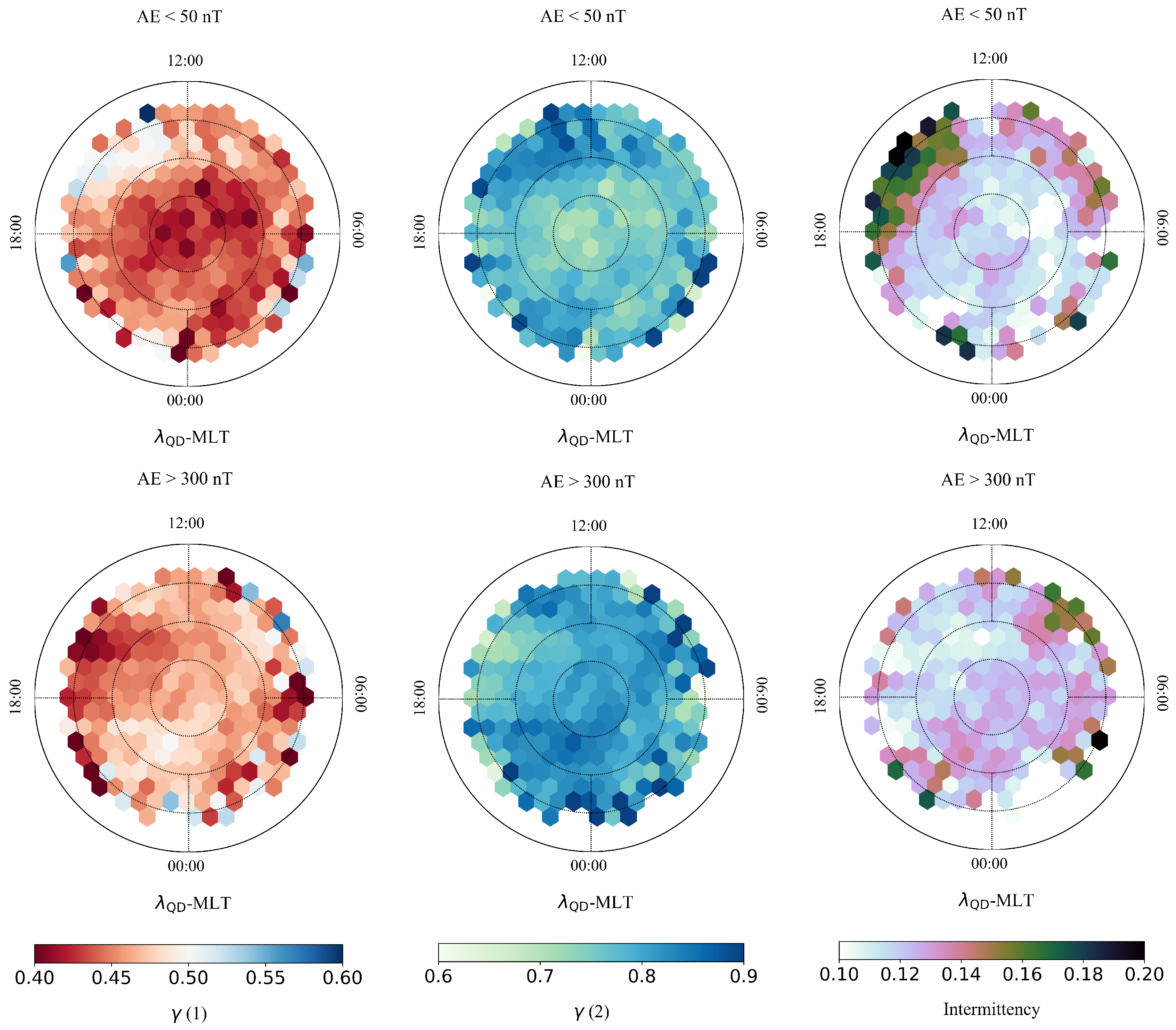
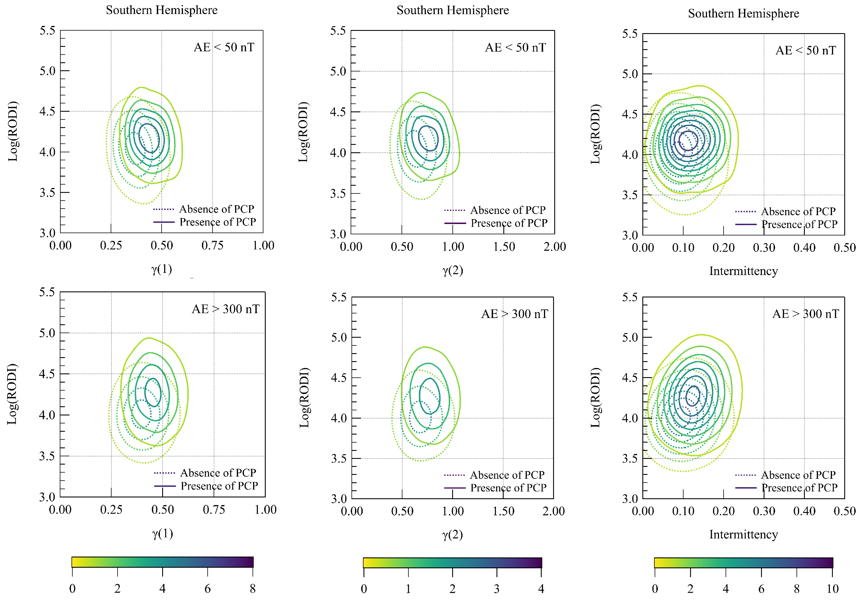
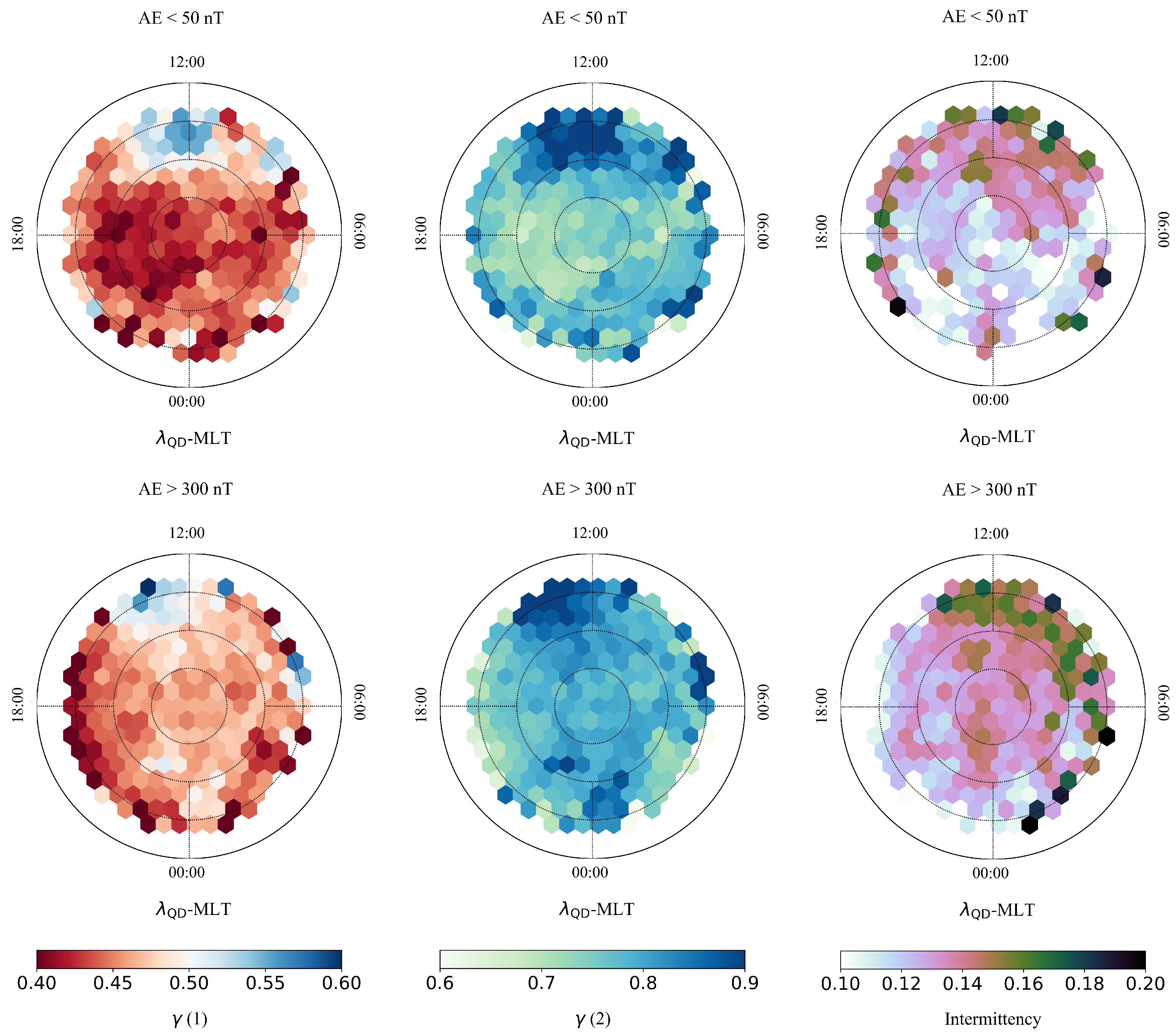
γ ( 2 ) gives information on the scaling features of the autocorrelation function and, most importantly, on the spectral features of the signal under investigation. Indeed, it can be demonstrated that in presence of a signal characterized by a power-law spectral density, i.e., ∼ f β (where f is frequency), its slope, β , is such that β = γ ( 2 ) + 1 [42].
As is well-known, spectral features can provide a strong indication on the occurrence of turbulent processes. To evaluate the scaling exponents we use the so-called Detrended Structure Function Analysis (DSFA) [43] since it has been proved to be the most reliable approach when dealing with measurements from satellites. The critical parameter to set for a correct application of DSFA is the width of the moving window over which the qth-order structure function defined in Equation (1) is estimated. The value of this parameter sets the maximum time scale τ max that can be resolved. In this case the width of the moving window is chosen to be of 40 s, a value that guarantees the statistical robustness of the computation of the qth-order scaling exponents. The minimum time scale τ min is, instead, dictated by the time series resolution—1 s in the case of the considered electron density dataset. Given these values of τ min and τ max , and considering that Swarm A satellite has an orbital velocity of ∼7.6 km/s, this method allows investigating ionospheric irregularities with spatial scales between approximately 8 and 400 km. These spatial scales are consistent with what shown in Figure 3. Technical details on DSFA method as well as on different kinds of its application on Swarm data can be found, e.g., in De Michelis et al. [20,28], Consolini et al. [44], to cite just a few. Moreover, the linear combination δ γ 2 , 1 of the first- and second-order scaling exponents, i.e.,
δ γ 2 , 1 = 2 γ ( 1 ) γ ( 2 )
provides a measure of the intermittent character of the fluctuations, i.e, of the occurrence of anomalous scaling features as observed in fluid and magnetohydrodynamic (MHD) turbulence [39,45]. Indeed, in the case of global scale invariance the scaling exponents, γ ( q ) are expected to have a linear dependence on the moment order q, i.e., γ ( q ) = γ ( 1 ) q , so that only one scaling exponent is sufficient to characterize the complexity of the fluctuation field. We remark that the quantity δ γ 2 , 1 is just a measure of the departure from a linear dependence of the scaling exponents on the moment order. A more exhaustive analysis of the intermittent character would require an extensive study of the convex nature of γ ( q ) on q. However, in what follows we will call the quantity in Equation (2) as intermittency, for brevity.

3. Results

After estimating the first- and second-order scaling exponents from Swarm A N e time series for the entire period under investigation, we divided values of γ ( 1 ) , γ ( 2 ) , intermittency and RODI into two subsets characterized by: (1) the presence of PCPs; (2) the absence of PCPs. Actually, when PCP flag values are equal to 4 or to 1, the first subset is obtained, while when they are equal to 0, the second subset is obtained.
A further selection criterion was applied to these subsets based on the AE index to distinguish between quiet and disturbed geomagnetic conditions. The entire analysis was performed separately for each hemisphere.
The idea of introducing RODI into our analysis arises from recent studies [19,46] that have highlighted how plasma bubbles, which are ionospheric irregularities occurring in equatorial regions, have a turbulent nature and are characterized by very high values of RODI. In that case, the analysis of the joint distribution between the scaling exponents inside the plasma bubbles and RODI has shown how the properties of this class of irregularities are completely different from the surrounding environment. Similarly, we examined the joint distribution between the scaling exponents and intermittency, and RODI, to investigate whether the properties of PCPs differ from the surrounding ionospheric environment. This investigation was carried out for both quiet and disturbed geomagnetic conditions in both polar regions. By doing so, we aimed to gain further insights into the distinctive characteristics and behavior of PCPs.
Joint probability distributions for the Northern hemisphere are shown in Figure 6. In detail, the upper plots show the results for quiet conditions for γ ( 1 ) (left side), γ ( 2 ) (center), and intermittency (right side), while the lower plots refer to disturbed conditions. Dotted lines represent joint probabilities distributions obtained for the absence of PCPs, while solid lines represent distributions obtained when PCPs are present. Figure 6 shows that the two distributions are shifted, on both axes, one with respect to the other. The shift of the isolines corresponding to the presence of PCPs on the vertical axis, i.e., towards higher values of log(RODI) can be explained in terms of the intrinsic meaning of RODI. Indeed, RODI is a measure of the presence of ionosphere irregularities, and PCPs are one among them. Therefore RODI values related to the presence of PCP are expected to be higher than those related to the absence of PCPs. The shift of the isolines corresponding to the presence of PCPs on the horizontal axes, for both γ ( 1 ) , γ ( 2 ) , and intermittency in the direction of higher values should instead be interpreted in terms of the different dynamical properties of PCPs with respect to the surrounding plasma. It is interesting to note that these distributions appear to be practically independent of the level of geomagnetic activity for both scaling exponents and intermittency.
The situation changes if we represent the values of the two scaling exponents as a function of QD-latitude and MLT separately for the two levels of geomagnetic activity as shown by Figure 7. Bins in Figure 7 represent, for the Northern hemisphere and both levels of geomagnetic activity, the average values of γ ( 1 ) (left side), γ ( 2 ) (center), and intermittency (right side) when the presence of PCP is recorded. Focusing on γ ( 1 ) , we see that under quiet geomagnetic conditions, only PCPs in the area corresponding to MLTs in the range 13:00–17:00 and to QD-latitudes between 75 and 80 , exhibit a weak persistent behavior with γ ( 1 ) > 0.5 . Differently, in this area, under disturbed conditions, values of γ ( 1 ) are primarily indicative of antipersistent behavior with γ ( 1 ) < 0.5 . At very high latitudes, i.e., larger than approximately 80 , the behavior of γ ( 1 ) suggests a decrease in antipersistency when moving from quiet to disturbed geomagnetic conditions. For what concerns γ ( 2 ) , higher values are observed in the areas characterized by a less antipersistent character. Looking back at the space distribution of PCPs in the Northern hemisphere under quiet and disturbed geomagnetic conditions (left side of Figure 5), we note that the areas with a high number of PCPs are characterized by a less antipersistent character (left side of Figure 7) and by higher values of γ ( 2 ) (center of Figure 7). When examining the spatial distribution of intermittency values, interesting observations can be made for periods of quiet geomagnetic conditions: high intermittency values are predominantly found in regions exhibiting a persistent behavior and high values of γ ( 2 ) . Specifically, these regions are concentrated on the dayside within a latitudinal range between approximately 75 and 80 . However, when geomagnetic activity increases, it is possible to observe a subtle shift in the spatial distribution of intermittency values. Indeed, high values tend to shift towards lower latitudes, while also extending to high latitudes during nighttime.
The analysis presented for the Northern hemisphere has also been repeated for the Southern hemisphere. The corresponding results demonstrate good agreement with those obtained in the Northern Hemisphere, as shown in Figure 8 and Figure 9. In Figure 8, we find again a split between joint probability distributions obtained in the two cases of presence and absence of PCPs, as well as the independence of these distributions from the level of geomagnetic activity. Furthermore, the peak values of the distributions related to the presence and absence of PCPs in the Northern and Southern hemispheres (for both levels of geomagnetic activity and both scaling exponents) are perfectly matching, indicating that the two hemispheres behave, in this regard, in a very similar manner. A slight difference can be observed in the spatial distribution of γ ( 1 ) , γ ( 2 ) , and intermittency values, as shown in Figure 9, compared to the findings in the Northern hemisphere. In the Southern hemisphere, the persistent behavior of the first-order scaling exponent occurs within a different MLT range (11:30–15:00) and exhibits slightly higher values than in the Northern hemisphere. Similarly, values of the second-order scaling exponent are slightly higher in the Southern hemisphere, with more localized high values. Moreover, the Southern hemisphere generally shows higher values of intermittency.
It is worth specifying here that we are aware that PCPs typically cover space scales from 100 to 1000 km and that the scaling exponents here estimated are capable of accurately describing the physical processes concerning patches with scale sizes up to a maximum of about 400 km. However, we are quite confident in the validity of the obtained results since Figure 3 quite robustly confirms that more than 65 % of identified PCPs used in this study have a size—which also includes the edges—smaller than 450 km.
To investigate the impact of PCPs on GNSS we conducted an analysis of LoL events recorded by Swarm A during the same 3.5-year interval (from 16 July 2014 to 28 February 2018) used so far. Indeed, as mentioned in Section 1, irregularities like these are often linked to a loss of signal from such systems. So, we directly identified GPS LoL events by detecting interruptions in the sTEC time series of each GPS satellite in the field of view of Swarm A. We considered as LoL events interruptions in the sTEC time series lasting between 2 and 1200 s. The duration of each LoL event was calculated by determining the difference between the timestamps corresponding to the beginning and the end of the identified sTEC interruption. For more details on the methodology, refer to Pezzopane et al. [24]. Then, we selected LoLs occurred simultaneously to PCPs and those occurred in absence of PCPs. Figure 10 displays the corresponding results. In detail, the upper plots represent LoL spatial distributions for the Northern hemisphere: on the left is the number of LoLs occurred in absence of PCPs (i.e., PCP flag equal to 0); on the right is the number of LoLs occurred in presence of PCPs (i.e., PCP flag equal to 1 or 4). The two bottom plots represent the histograms indicating how the number of LoLs occurring in presence (red) and in absence (gray) of PCPs varies with QD-latitude (left) and MLT (right).
As indicated by the percentage shown in the bottom right corner of each map in the upper part of Figure 10, more than half of the events coincide with PCPs. The events coinciding with PCPs exhibit a spatial distribution characterized by a peak in the range of QD-latitudes 80 ÷ 85 , mainly at MLTs between around 05:00 and 10:00 MLT. In contrast, the LoLs not coinciding with PCPs have a more uniform distribution.
The same analysis was conducted for the Southern hemisphere, as shown in Figure 11. Here, the percentage of LoL events coinciding with PCPs is around one-third of the total number of events, which is therefore lower than in the Northern hemisphere. The plot on the top right of Figure 11, showing the spatial distribution of LoLs coinciding with PCPs (in the red-scale map), exhibits only one main peak in the dayside sector, between approximately 11:00 and 17:00 MLT. Differently from the Northern hemisphere, distributions in gray shown in the bottom part of Figure 11, i.e., of LoLs occurring in absence of PCPs does not display the almost uniform character displayed in Figure 10.
Finally, we compared the joint distribution between RODI and γ ( 2 ) obtained considering all LoL events and all PCPs. Figure 12 shows the results for both hemispheres and the two levels of geomagnetic activity. The upper plots display the distributions during quiet periods, while the bottom plots show the distributions during disturbed conditions. Contours of the joint distribution associated with LoLs (indicated by dashed contours) are shifted towards higher values of RODI compared to those associated with PCPs (indicated by solid contours). The displacement of the two distributions with respect to γ ( 2 ) is not as pronounced as the displacement with respect to RODI, especially during disturbed periods, likely due to the similar dynamical properties characterizing the two phenomena. The area where the two distributions overlap provides a rough indication of LoLs occurring in presence of PCPs. Precisely, during periods of low geomagnetic activity, 51.4 % of LoL events coincide with PCPs, a percentage which increases to 57.4 % for AE > 300 nT. In contrast, for the Southern hemisphere, only 20.1 % of all LoL events for AE < 50 nT coincide with PCPs, a percentage which significantly increases to 45.7 % during high geomagnetic activity periods.

4. Discussion and Conclusions

The high-latitude ionosphere is characterized by the presence of multi-scale structures that becomes clear when studying the dynamic processes that occur on mesoscales, which means on spatial scales ranging from tens to hundreds of kilometers. These structures are created by different types of plasma instabilities and other processes that are essentially responsible for variations in plasma density and electric fields. Transient and localized structures can often be observed in regions such as the cusp, polar cap, and auroral oval, whose properties, propagation, and coupling processes are not yet fully understood, although they represent a critical element in the development of realistic numerical models. The results just presented fall within this scope and aim to shed new light on the properties of a particular type of plasma irregularity, the polar cap patch, which can be analyzed using electron density data measured by a low-altitude polar-orbiting satellite belonging to the ESA Swarm constellation. The analysis of the scale properties of electron density fluctuations shows that there is some difference between what is found within these irregularities and the surrounding environment. Indeed, electron density fluctuations corresponding to PCPs are associated with higher average values of RODI and have a less antipersistent character than those not corresponding to PCPs. This difference with the surrounding environment can be observed during both quiet and disturbed conditions. Concerning the second-order scaling exponent, which indirectly provides information on the values of the slope of the fluctuations’ energy spectrum, the PCPs are characterized by higher values compared to the external environment. Inside the PCPs, the second-order scaling exponent is between 0.8 and 0.9, which means a slope β of the energy spectrum of between 1.8 and 1.9. The electron density fluctuations outside the PCPs have a second-order scaling exponent of about 0.7 and therefore an energy spectrum slope value of β 1.7 . Thus, we can infer a distinct electron density fluctuation dynamics from the difference in the second-order scaling exponent values inside and outside the irregular structures analyzed. Additionally, the power spectral indices obtained indirectly can aid in identifying instabilities responsible for low-frequency turbulence [47]. These findings are consistent with previous research that utilized data from other satellites and demonstrated that the power spectra of increased plasma density fluctuations typically follow a power law with a spectral index β 1.8 [48,49,50] for scales ranging from several kilometers to tens of meters. These spectra were linked to the gradient drift instability (e.g., [51]), which arises from the differential drifts of ions and electrons on a plasma density gradient, and to the Kelvin–Helmholtz instability, which occurs in the presence of flow shears (e.g., [5,49]). In conclusion, the statistical analysis of PCPs conducted on approximately 3.5 years of data clearly shows that these structures, with respect to the surrounding environment, are characterized by electron density fluctuations with higher values of γ ( 1 ) and a steeper energy spectrum that can be associated with the occurrence of gradient drift instability and Kelvin–Helmholtz instability, and higher RODI values, meaning they are characterized by larger density fluctuations. These characteristics are independent of the hemisphere in which the PCPs develop. Beyond what resulting considering the whole set of PCPs that allowed us to obtain their average characterization and, at the same time, provided us with a tool to distinguish them from the surrounding environment, the results reported in Figure 7 and Figure 9 are certainly very interesting. These results show how the scaling properties of PCPs tend to vary according to their spatial location within the analyzed region, which corresponds to magnetic latitudes greater than | 75 | .
Let us start by analyzing the spatial distributions of the values of the two scale exponents during geomagnetic quiet periods in both hemispheres, referring to the maps shown in the top panels of Figure 7 and Figure 9. What immediately becomes clear is how the scale properties of electron density fluctuations present on the dayside tend to have values of both scale exponents higher than those of other regions. Considering the spatial location, it is immediately clear that this region identifies the cusp. The cusp is a region that extends for a few hours of MLT and whose position is a function of the y and z components of the interplanetary magnetic field. It is characterized by the continuous precipitation of ions and electrons of external origin and it is therefore one of the regions most directly dependent on changes in solar wind conditions. The continuous precipitation of particles gives rise to a series of localized and transient structures, some of which may be triggered by changes in the orientation of the interplanetary magnetic field. The electron density measurements collected by the Swarm A satellite seem to indicate the presence of PCPs in this region, although not in large quantities (see Figure 5). This confirms previous studies [52], which noted that patches can be associated with weak soft electron precipitation. This suggests that PCPs are associated with flux tubes formed by open field lines, and therefore should exhibit different properties from those of the surrounding plasma that is not directly connected to the solar wind. The scaling features of these plasma density irregularities are also consistent with the analysis presented by Spicher et al. [53], who studied electron density data from the ICI-2 (Investigation of Cusp Irregularities-2) sounding rocket experiment in the high-latitude F region. They found that plasma enhancements subjected to soft particle precipitation displayed stronger random features with uncorrelated phases of density fluctuations, indicating that particle precipitation played a critical role in structuring the ionospheric plasma and creating turbulent-like structures. The only other region where similar properties to those found in the cusp can be observed, albeit less clearly, is around midnight at a magnetic latitude near 75 .
If we now focus on what happens during periods of high geomagnetic activity (bottom panels of Figure 7 and Figure 9), we observe that the highest values of the second-order scaling exponent are found not only in the cusp region, but in this case, they involve the entire polar cap reaching the nighttime sector. Considering the structure of high-latitude convection cells and the motion of the plasma associated with them, it becomes clear that the regions characterized by higher values of the second-order scale exponent correspond to the area in between the two convection cells, generally characterized by an antisunward flow. When different layers of plasma move at different speeds or in different directions, shear layers can be created where the plasma flows are unstable and generate turbulence. This type of turbulence is the so-called shear-flow turbulence. On the other hand, where the plasma density changes rapidly over a short distance, the ions and electrons in the plasma experience different drift velocities due to the gradient and this creates a current that can generate electromagnetic waves and, under certain conditions, can become unstable and generate turbulence. Thus, both velocity shear and plasma density gradients are types of instabilities that can lead to the formation of plasma irregularities in the ionosphere, and in particular at high-latitudes. All of the regions with higher values of the second-order scaling exponent also have higher values of the first-order scaling exponent, indicating that the plasma density fluctuations have a more persistent character. This feature is shared by both hemispheres, though it is more visible in the Southern hemisphere. Therefore, the analysis carried out in this study has revealed that the electron density fluctuations within the PCPs, identified using a Swarm Level 2 product, exhibit scale characteristics that differ from those found by analyzing the same fluctuations outside these irregularities. In general, PCPs are characterized by higher values of both scaling exponents and RODI. These differences are accentuated with the intensification of geomagnetic activity and are mainly concentrated in the cusp and in the region of separation between the two convective cells. It is worth noting that PCPs form in an ionospheric environment that differs significantly from the one where plasma bubbles develop, while the scale properties of electron density fluctuations inside plasma bubbles are completely different from the surrounding environment, with a second-order scaling exponent value of ( 0.98 ± 0.21 ) inside the bubbles and around 2 in the surrounding area [19]. The RODI values are also markedly different, increasing by over one order of magnitude inside the bubbles [19,21]. Conversely, the scaling properties inside (including PCPs’ borders) and outside PCPs are similar indicating a state of widespread turbulence in the ionospheric region under investigation, which is absent in the equatorial ionospheric region.
During GPS LoL events recorded by the Swarm constellation, a notable difference in scaling properties and higher values of RODI compared to the surrounding environment were observed in the plasma density irregularities [21]. To gain a deeper understanding of the impact of PCPs on GPS signal propagation, we conducted an analysis to assess how the irregularities at the base of LoL events are attributable to PCPs. Our findings reveal that a significant percentage of LoL events occurring over 74 of QD-latitude coincided with PCPs. This was the case for over half of the events (∼55%) in the Northern hemisphere and approximately one third (∼33%) in the Southern hemisphere. The coincidence actually increases to approximately 57.4 % in the Northern hemisphere and 45.7 % in the Southern hemisphere during periods when AE > 300 nT. The difference between the two hemispheres could be ascribed to the varying occurrence of PCPs. Interestingly, despite a lower occurrence of PCPs, the number of LoLs is higher in the Southern hemisphere [24]. Overall, PCPs are confirmed as ionospheric irregularities that actively contribute to the loss of electromagnetic signals propagating through the ionosphere. However, a complete overlap between the presence of these irregularities and the occurrence of LoLs is not observed. The comparison of joint distributions between RODI and γ ( 2 ) for ionospheric irregularities associated with PCPs and LoL events (Figure 12) highlights that only PCPs with significantly high RODI values have the potential to trigger a LoL event.

Author Contributions

Conceptualization, R.T. and P.D.M.; methodology, G.C.; formal analysis, R.T. and G.L.; investigation, R.T. and G.L.; data curation, R.T., G.C. and A.P.; writing—original draft preparation, R.T., P.D.M. and G.L.; writing—review and editing, all authors; project administration, P.D.M. All authors have read and agreed to the published version of the manuscript.

Funding

This research received financial support from the Italian PNRA under contract PNRA18_002 89-A “Space weather in Polar Ionosphere: the Role of Turbulence”.

Data Availability Statement

Swarm data can be accessed at http://swarm-diss.eo.esa.int (accessed on 31 August 2023). AE index is freely available at https://wdc.kugi.kyoto-u.ac.jp/ae_provisional/index.html (accessed on 31 August 2023).

Acknowledgments

The results presented rely on data collected by ESA-Swarm mission. We thank the European Space Agency that supports the Swarm mission. The results presented in this paper rely on AE geomagnetic index calculated and made available by the Kyoto WDC for Geomagnetism from data collected at magnetic observatories. We thank the involved national institutes, the INTERMAGNET network, and ISGI (https://isgi.unistra.fr/). G.L. acknowledges the PhD course in Astronomy, Astrophysics and Space Science of the University of Rome “Sapienza”, University of Rome “Tor Vergata”, and Istituto Nazionale di Geofisica e Vulcanologia, Italy.

Conflicts of Interest

The authors declare no conflict of interest. The funders had no role in the design of the study; in the collection, analyses, or interpretation of data; in the writing of the manuscript; or in the decision to publish the results.

Abbreviations

The following abbreviations are used in this manuscript:
AEAuroral Electrojet
CDFCumulative Distribution Function
CHAMPChallenging Minisatellite Payload
DSFADetrended Structure Function Analysis
ESAEuropean Space Agency
EUVExtreme Ultra Violet
GLONASSGlobalnaya Navigazionnaya Sputnikovaya Sistema
GNSSGlobal Navigation Satellite System
GPSGlobal Positioning System
ICI-2Investigation of Cusp Irregularities-2
INTERMAGNETInternational Real-time Magnetic Observatory Network
ISGIInternational Service of Geomagnetic Indices
LoLLoss of Lock
MHDMagnetohydrodynamics
MLTMagnetic Local Time
PCPPolar Cap Patch
PDFProbability Density Function
QDQuasi-Dipole
RODIRate Of change of electron Density Index
sTECslant Total Electron Content
TITIPyTopside Ionosphere Turbulence Indices with Python
WDCWorld Data Center

References

  1. Tsunoda, R.T. High-latitude F region irregularities: A review and synthesis. Rev. Geophys. 1988, 26, 719–760. [Google Scholar] [CrossRef]
  2. Balan, N.; Liu, L.; Le, H. A brief review of equatorial ionization anomaly and ionospheric irregularities. Earth Planet. Phys. 2018, 2, 257. [Google Scholar] [CrossRef]
  3. Jin, Y.; Xiong, C.; Clausen, L.; Spicher, A.; Kotova, D.; Brask, S.; Kervalishvili, G.; Stolle, C.; Miloch, W. Ionospheric Plasma Irregularities Based on In Situ Measurements From the Swarm Satellites. J. Geophys. Res. Space Phys. 2020, 125, e2020JA028103. [Google Scholar] [CrossRef]
  4. Bhattacharyya, A. Equatorial Plasma Bubbles: A Review. Atmosphere 2022, 13, 1637. [Google Scholar] [CrossRef]
  5. Carlson, H.C. Sharpening our thinking about polar cap ionospheric patch morphology, research, and mitigation techniques. Radio Sci. 2012, 47, 1–6. [Google Scholar] [CrossRef]
  6. Clausen, L.B.N.; Moen, J.I. Electron density enhancements in the polar cap during periods of dayside reconnection. J. Geophys. Res. Space Phys. 2015, 120, 4452–4464. [Google Scholar] [CrossRef]
  7. Lockwood, M.; Carlson, H.C., Jr. Production of polar cap electron density patches by transient magnetopause reconnection. Geophys. Res. Lett. 1992, 19, 1731–1734. [Google Scholar] [CrossRef]
  8. Dungey, J.W. Interplanetary Magnetic Field and the Auroral Zones. Phys. Rev. Lett. 1961, 6, 47–48. [Google Scholar] [CrossRef]
  9. Jin, Y.; Spicher, A.; Xiong, C.; Clausen, L.B.N.; Kervalishvili, G.; Stolle, C.; Miloch, W.J. Ionospheric Plasma Irregularities Characterized by the Swarm Satellites: Statistics at High Latitudes. J. Geophys. Res. Space Phys. 2019, 124, 1262–1282. [Google Scholar] [CrossRef]
  10. Basu, S.; Basu, S.; Chaturvedi, P.K.; Bryant, C.M., Jr. Irregularity structures in the cusp/cleft and polar cap regions. Radio Sci. 1994, 29, 195–207. [Google Scholar] [CrossRef]
  11. Lorentzen, D.A.; Moen, J.; Oksavik, K.; Sigernes, F.; Saito, Y.; Johnsen, M.G. In situ measurement of a newly created polar cap patch. J. Geophys. Res. Space Phys. 2010, 115, A12323. [Google Scholar] [CrossRef]
  12. Moen, J.; Oksavik, K.; Abe, T.; Lester, M.; Saito, Y.; Bekkeng, T.A.; Jacobsen, K.S. First in-situ measurements of HF radar echoing targets. Geophys. Res. Lett. 2012, 39, L07104. [Google Scholar] [CrossRef]
  13. Goodwin, L.V.; Iserhienrhien, B.; Miles, D.M.; Patra, S.; van der Meeren, C.; Buchert, S.C.; Burchill, J.K.; Clausen, L.B.N.; Knudsen, D.J.; McWilliams, K.A.; et al. Swarm in situ observations of F region polar cap patches created by cusp precipitation. Geophys. Res. Lett. 2015, 42, 996–1003. [Google Scholar] [CrossRef]
  14. Spicher, A.; Cameron, T.; Grono, E.M.; Yakymenko, K.N.; Buchert, S.C.; Clausen, L.B.N.; Knudsen, D.J.; McWilliams, K.A.; Moen, J.I. Observation of polar cap patches and calculation of gradient drift instability growth times: A Swarm case study. Geophys. Res. Lett. 2015, 42, 201–206. [Google Scholar] [CrossRef]
  15. Noja, M.; Stolle, C.; Park, J.; Lühr, H. Long-term analysis of ionospheric polar patches based on CHAMP TEC data. Radio Sci. 2013, 48, 289–301. [Google Scholar] [CrossRef]
  16. Burston, R.; Mitchell, C.; Astin, I. Polar cap plasma patch primary linear instability growth rates compared. J. Geophys. Res. Space Phys. 2016, 121, 3439–3451. [Google Scholar] [CrossRef]
  17. Spicher, A.; Clausen, L.B.N.; Miloch, W.J.; Lofstad, V.; Jin, Y.; Moen, J.I. Interhemispheric study of polar cap patch occurrence based on Swarm in situ data. J. Geophys. Res. Space Phys. 2017, 122, 3837–3851. [Google Scholar] [CrossRef]
  18. Keskinen, M.J.; Ossakow, S. Non-linear evolution of plasma enhancements in the auroral ionosphere 1. Long wavelength irregularities. J. Geophys. Res. Space Phys. 1982, 87, 144–150. [Google Scholar] [CrossRef]
  19. De Michelis, P.; Consolini, G.; Tozzi, R.; Pignalberi, A.; Pezzopane, M.; Coco, I.; Giannattasio, F.; Marcucci, M.F. Ionospheric Turbulence and the Equatorial Plasma Density Irregularities: Scaling Features and RODI. Remote Sens. 2021, 13, 759. [Google Scholar] [CrossRef]
  20. De Michelis, P.; Consolini, G.; Pignalberi, A.; Tozzi, R.; Coco, I.; Giannattasio, F.; Pezzopane, M.; Balasis, G. Looking for a proxy of the ionospheric turbulence with Swarm data. Sci. Rep. 2021, 11, 6183. [Google Scholar] [CrossRef]
  21. De Michelis, P.; Consolini, G.; Pignalberi, A.; Lovati, G.; Pezzopane, M.; Tozzi, R.; Giannattasio, F.; Coco, I.; Marcucci, M.F. Ionospheric Turbulence: A Challenge for GPS Loss of Lock Understanding. Space Weather 2022, 20, e2022SW003129. [Google Scholar] [CrossRef]
  22. Friis-Christensen, E.; Lühr, H.; Hulot, G. Swarm: A constellation to study the Earth’s magnetic field. Earth Planets Space 2006, 58, 351–358. [Google Scholar] [CrossRef]
  23. Knudsen, D.J.; Burchill, J.K.; Buchert, S.C.; Eriksson, A.I.; Gill, R.; Wahlund, J.E.; Åhlen, L.; Smith, M.; Moffat, B. Thermal ion imagers and Langmuir probes in the Swarm electric field instruments. J. Geophys. Res. Space Phys. 2017, 122, 2655–2673. [Google Scholar] [CrossRef]
  24. Pezzopane, M.; Pignalberi, A.; Coco, I.; Consolini, G.; De Michelis, P.; Giannattasio, F.; Marcucci, M.F.; Tozzi, R. Occurrence of GPS Loss of Lock Based on a Swarm Half-Solar Cycle Dataset and Its Relation to the Background Ionosphere. Remote Sens. 2021, 13, 2209. [Google Scholar] [CrossRef]
  25. Lomidze, L.; Knudsen, D.J.; Burchill, J.; Kouznetsov, A.; Buchert, S.C. Calibration and Validation of Swarm Plasma Densities and Electron Temperatures Using Ground-Based Radars and Satellite Radio Occultation Measurements. Radio Sci. 2018, 53, 15–36. [Google Scholar] [CrossRef]
  26. Swarm L1b Product Definition. Available online: https://earth.esa.int/documents/10174/1514862/Swarm_L1b_Product_Definition (accessed on 31 August 2023).
  27. Zakharenkova, I.; Astafyeva, E. Topside ionospheric irregularities as seen from multisatellite observations. J. Geophys. Res. Space Phys. 2015, 120, 807–824. [Google Scholar] [CrossRef]
  28. De Michelis, P.; Pignalberi, A.; Consolini, G.; Coco, I.; Tozzi, R.; Pezzopane, M.; Giannattasio, F.; Balasis, G. On the 2015 St. Patrick’s Storm Turbulent State of the Ionosphere: Hints From the Swarm Mission. J. Geophys. Res. Space Phys. 2020, 125, e2020JA027934. [Google Scholar] [CrossRef]
  29. Piersanti, M.; De Michelis, P.; Del Moro, D.; Tozzi, R.; Pezzopane, M.; Consolini, G.; Marcucci, M.F.; Laurenza, M.; Di Matteo, S.; Pignalberi, A.; et al. From the Sun to Earth: Effects of the 25 August 2018 geomagnetic storm. Ann. Geophys. 2020, 38, 703–724. [Google Scholar] [CrossRef]
  30. Pignalberi, A. TITIPy: A Python tool for the calculation and mapping of topside ionosphere turbulence indices. Comput. Geosci. 2021, 148, 104675. [Google Scholar] [CrossRef]
  31. Jin, Y.; Kotova, D.; Xiong, C.; Brask, S.M.; Clausen, L.B.N.; Kervalishvili, G.; Stolle, C.; Miloch, W.J. Ionospheric Plasma IRregularities-IPIR-Data product based on data from the Swarm satellites. J. Geophys. Res. Space Phys. 2022, 127, e2021JA030183. [Google Scholar] [CrossRef] [PubMed]
  32. Swarm Product Specification for L2 Products and Auxiliary Products. Available online: https://earth.esa.int/eogateway/documents/20142/37627/swarm-level-2-product-specification.pdf/2979b351-b6a2-69b6-8539-9ed9f32984f0 (accessed on 31 August 2023).
  33. Swarm Handbook—Level 2 Product Definitions Introduction. Available online: https://swarmhandbook.earth.esa.int/article/introduction#:~:text=Level%202%20products%20are%20typically,well%20as%20ground%2Dbased%20observations (accessed on 31 August 2023).
  34. Coley, W.R.; Heelis, R.A. Adaptive identification and characterization of polar ionization patches. J. Geophys. Res. Space Phys. 1995, 100, 23819–23827. [Google Scholar] [CrossRef]
  35. Chartier, A.T.; Mitchell, C.N.; Miller, E.S. Annual Occurrence Rates of Ionospheric Polar Cap Patches Observed Using Swarm. J. Geophys. Res. Space Phys. 2018, 123, 2327–2335. [Google Scholar] [CrossRef]
  36. Kagawa, A.; Hosokawa, K.; Ogawa, Y.; Ebihara, Y.; Kadokura, A. Occurrence Distribution of Polar Cap Patches: Dependences on UT, Season and Hemisphere. J. Geophys. Res. Space Phys. 2020, 126, e2020JA028538. [Google Scholar] [CrossRef]
  37. David, M.; Sojka, J.; Schunk, R.; Coster, A. Hemispherical Shifted Symmetry in Polar Cap Patch Occurrence: A Survey of GPS TEC Maps From 2015–2018. Geophys. Res. Lett. 2019, 46, 10726–10734. [Google Scholar] [CrossRef]
  38. Davis, T.N.; Sugiura, M. Auroral electrojet activity index AE and its universal time variations. J. Geophys. Res. 1966, 71, 785–801. [Google Scholar] [CrossRef]
  39. Frisch, U. Turbulence: The Legacy of A. N. Kolmogorov; Cambridge University Press: Cambridge, UK, 1995. [Google Scholar]
  40. Taylor, G.I. The Spectrum of Turbulence. Proc. R. Soc. Lond. Ser. A-Math. Phys. Sci. 1938, 164, 476–490. [Google Scholar] [CrossRef]
  41. Hurst, H.E. Methods of using long-term storage in reservoirs. Proc. Inst. Civ. Eng. 1956, 5, 519–543. [Google Scholar] [CrossRef]
  42. Wiener, N. Time Series; M.I.T. Press: Cambridge, MA, USA, 1964; p. 42. [Google Scholar]
  43. De Michelis, P.; Consolini, G.; Tozzi, R. Magnetic field fluctuation features at Swarm’s altitude: A fractal approach. Geophys. Res. Lett. 2015, 42, 3100–3105. [Google Scholar] [CrossRef]
  44. Consolini, G.; Tozzi, R.; De Michelis, P.; Coco, I.; Giannattasio, F.; Pezzopane, M.; Marcucci, M.; Balasis, G. High-latitude polar pattern of ionospheric electron density: Scaling features and IMF dependence. J. Atmos. Sol.-Terr. Phys. 2021, 217, 105531. [Google Scholar] [CrossRef]
  45. Bruno, R.; Carbone, V. The Solar Wind as a Turbulence Laboratory. Living Rev. Sol. Phys. 2013, 10, 2. [Google Scholar] [CrossRef]
  46. De Michelis, P.; Consolini, G.; Alberti, T.; Tozzi, R.; Giannattasio, F.; Coco, I.; Pezzopane, M.; Pignalberi, A. Magnetic Field and Electron Density Scaling Properties in the Equatorial Plasma Bubbles. Remote Sens. 2022, 14, 918. [Google Scholar] [CrossRef]
  47. Kintner, P.M.; Seyler, C.E. The status of observations and theory of high latitude ionospheric and magnetospheric plasma turbulence. Space Sci. Rev. 1985, 41, 91–129. [Google Scholar] [CrossRef]
  48. Basu, S.; Basu, S.; MacKenzie, E.; Fougere, P.F.; Coley, W.R.; Maynard, N.C.; Winningham, J.D.; Sugiura, M.; Hanson, W.B.; Hoegy, W.R. Simultaneous density and electric field fluctuation spectra associated with velocity shears in the auroral oval. J. Geophys. Res. 1988, 93, 115–136. [Google Scholar] [CrossRef]
  49. Basu, S.; MacKenzie, E.; Basu, S.; Coley, W.R.; Sharber, J.R.; Hoegy, W.R. Plasma structuring by the gradient drift instability at high latitudes and comparison with velocity shear driven processes. J. Geophys. Res. 1990, 95, 7799–7818. [Google Scholar] [CrossRef]
  50. Dyson, P.L.; McClure, J.P.; Hanson, W.B. In situ measurements of the spectral characteristics of F region ionospheric irregularities. J. Geophys. Res. 1974, 79, 1497. [Google Scholar] [CrossRef]
  51. Cerisier, J.C.; Berthelier, J.J.; Beghin, C. Unstable density gradients in the high-latitude ionosphere. Radio Sci. 1985, 20, 755–761. [Google Scholar] [CrossRef]
  52. Zou, Y.; Nishimura, Y.; Lyons, L.R.; Shiokawa, K. Localized polar cap precipitation in association with nonstorm time airglow patches. Geophys. Res. Lett. 2017, 44, 609–617. [Google Scholar] [CrossRef]
  53. Spicher, A.; Miloch, W.J.; Clausen, L.B.N.; Moen, J.I. Plasma turbulence and coherent structures in the polar cap observed by the ICI-2 sounding rocket. J. Geophys. Res. Space Phys. 2015, 120, 10959–10978. [Google Scholar] [CrossRef]
Figure 1. Time distribution of all PCPs identified between 16 July 2014 and 28 February 2018 from Swarm A. Left side refers to the Northern hemisphere while right side to the Southern one. Blue solid line represents the monthly sunspot number.
Remotesensing 15 04320 g001
Figure 2. Space distribution of all PCPs identified between 16 July 2014 and 28 February 2018 from Swarm A PCP flag as a function of QD-latitude ( λ QD ) and magnetic local time (MLT). Left side refers to the Northern hemisphere while right side to the Southern one. Circles are drawn at QD-latitudes of 70 , 75 , 80 , and 85 .
Remotesensing 15 04320 g002
Figure 3. Cumulative distribution function (CDF) and probability density function (PDF) of the size x of PCPs as identified by Swarm A PCP flag from the period 16 July 2014–28 February 2018. The blue line represents the CDF; red bars represent the PDF.
Remotesensing 15 04320 g003
Figure 4. Time distribution of the PCPs identified between 16 July 2014 and 28 February 2018 from Swarm A under different geomagnetic conditions. Top: PCPs observed during quiet geomagnetic conditions (AE < 50 nT); bottom, PCPs observed during disturbed geomagnetic conditions (AE > 300 nT). Left side refers to the Northern hemisphere while right side to the Southern one. Blue solid line represents the monthly sunspot number.
Remotesensing 15 04320 g004
Figure 5. Space distribution of PCPs as a function of QD-latitude ( λ QD ) and magnetic local time (MLT), for two levels of geomagnetic activity, i.e., quiet for AE < 50 nT (upper panels) and disturbed for AE > 300 nT (lower panels). Left side refers to the Northern hemisphere while right side to the Southern one. Circles are drawn at QD-latitudes of 70 , 75 , 80 , and 85 .
Remotesensing 15 04320 g005
Figure 6. Northern hemisphere: joint probability distributions between RODI and γ ( 1 ) (left side), γ ( 2 ) (center), and intermittency (right side) separately for data with (solid contours) and without (dashed contours) PCPs, for two levels of geomagnetic activity, i.e., quiet (top) and disturbed (bottom).
Remotesensing 15 04320 g006
Figure 7. Northern hemisphere: space distribution of the values of γ ( 1 ) (left side), γ ( 2 ) (center), and intermittency (right side) corresponding to the presence of PCPs as a function of QD-latitude ( λ QD ) and magnetic local time (MLT), for two levels of geomagnetic activity, i.e., quiet (top) and disturbed (bottom). Circles are drawn at QD-latitudes of 70 , 75 , 80 , and 85 .
Remotesensing 15 04320 g007
Figure 8. Southern hemisphere: joint probability distributions between RODI and γ ( 1 ) (left side), γ ( 2 ) (center), and intermittency (right side) separately for data with (solid contours) and without (dashed contours) PCPs, for two levels of geomagnetic activity, i.e., quiet (top) and disturbed (bottom).
Remotesensing 15 04320 g008
Figure 9. Southern hemisphere: space distribution of the values of γ ( 1 ) (left side), γ ( 2 ) (center), and intermittency (right side) corresponding to the presence of PCPs as a function of QD-latitude ( λ QD ) and magnetic local time (MLT), for two levels of geomagnetic activity, i.e., quiet (top) and disturbed (bottom). Circles are drawn at QD-latitudes of 70 , 75 , 80 , and 85 .
Remotesensing 15 04320 g009
Figure 10. Northern Hemisphere. Top: spatial distribution of LoL events occurring in the presence (right) and absence (left) of PCPs as a function of QD-latitude ( λ QD ) and magnetic local time (MLT). Circles are drawn at QD-latitudes of 70 , 75 , 80 , and 85 . The percentage at the bottom right of each plot indicates the percentage of LoLs coinciding and not coinciding with PCPs. Circles are drawn at QD-latitudes of 70 , 75 , 80 , and 85 . Bottom: distribution of LoL events as a function of QD-latitude ( λ QD ) (left) and MLT (right). Gray indicates LoLs occurring in absence of PCPs, red indicates LoLs occurring in the presence of PCPs.
Remotesensing 15 04320 g010
Figure 11. Southern Hemisphere. Top: spatial distribution of LoL events occurring in the presence (right) and absence (left) of PCPs as a function of QD-latitude ( λ QD ) and magnetic local time (MLT). Circles are drawn at QD-latitudes of 70 , 75 , 80 , and 85 . The percentage at the bottom right of each plot indicates the percentage of LoLs coinciding and not coinciding with PCPs. Circles are drawn at QD-latitudes of 70 , 75 , 80 , and 85 . Bottom: distribution of LoL events as a function of QD-latitude ( λ QD ) (left) and MLT (right). Gray indicates LoLs occurring in absence of PCPs, red indicates LoLs occurring in the presence of PCPs.
Remotesensing 15 04320 g011
Figure 12. Joint probability distributions between RODI and γ ( 2 ) associated with PCPs (solid contours, color scale is the same used in Figure 6 and Figure 8) and LoL events (dashed contours), for two levels of geomagnetic activity (quiet on top and disturbed on bottom), in the Northern hemisphere (left) and Southern hemisphere (right).
Remotesensing 15 04320 g012
Disclaimer/Publisher’s Note: The statements, opinions and data contained in all publications are solely those of the individual author(s) and contributor(s) and not of MDPI and/or the editor(s). MDPI and/or the editor(s) disclaim responsibility for any injury to people or property resulting from any ideas, methods, instructions or products referred to in the content.

