A Quasi-Coherent Detection Method Based on Radon–Fourier Transform Using Multi-Frequency-Based Passive Bistatic Radar

Abstract

Passive bistatic radar (PBR)-based moving target detection (MTD) has benefited greatly from multi-frequency (MF) integration, which can effectively improve the detection capability of weak targets. However, with the increase in the coherent processing interval (CPI) and carrier-frequency separation, Doppler spread will appear in the range-Doppler maps (RDMs) over different frequency bands, which severely limits the processing gain of MF integration. In this paper, a novel MTD algorithm is proposed to achieve both long-time integration and quasi-coherent MF integration. More specifically, the proposed method consists of two main steps, where a modified Radon–Fourier transform (RFT), termed as MF-based RFT (MF-RFT), is, firstly, used to eliminate the Doppler spread via designing a sequential of MF-based Doppler filter banks. Following the MF-RFT, a phase-compensation-based method is also developed to further remove the residual phase errors. This method involves formulating an optimization problem based on the minimum-entropy criterion and employing a particle swarm optimization (PSO) algorithm to solve it, after which quasi-coherent MF integration can be achieved with robustness. Both numerical results and field test results based on digital video broadcasting-satellite (DVB-S) signals demonstrate that the proposed algorithm outperforms the existing methods in the scenario of weak MTD.

1. Introduction

Recently, passive bistatic radar (PBR) has received renewed and increasing interest due to its capability of silent surveillance [1]. The absence of a transmitter enables PBR to avoid spectrum occupancy and realize target detection by exploiting the existing illuminators of opportunity (IOs), such as frequency-modulated (FM)-based broadcast [2], as well as digital transmissions, such as global systems for mobile communication (GSMs) [3], digital audio broadcasting (DAB) [4], digital video broadcasting—terrestrial (DVB-T) [5], digital video broadcasting—satellite (DVB-S) [6], global navigation satellite system (GNSS) signal [7], and the 5G network [8]. Various PBR systems have been developed and employed for shorter-range monitoring applications to detect small drones, vehicles, and people, or for remote area surveillance [1]. When the IOs exhibit several regular frequency bands emitted by a single transmitter, further performance improvements can be achieved via exploiting multi-frequency integration (MFI) [9].

So far, MFI techniques have been widely applied in various IOs, such as FM broadcast signals [10], DVB-T signals [11], and DVB-S signals [12]. Among them, DVB-S, as a satellite-based IO, can provide a high range resolution of several meters and continental coverage [13]. Therefore, it is a promising IO and has been widely applied to detect unmanned aerial vehicles (UAVs) [14], offshore vessels [15], and ground vehicles [16,17]. Hence, this article selects the DVB-S signal as the IO for investigation.

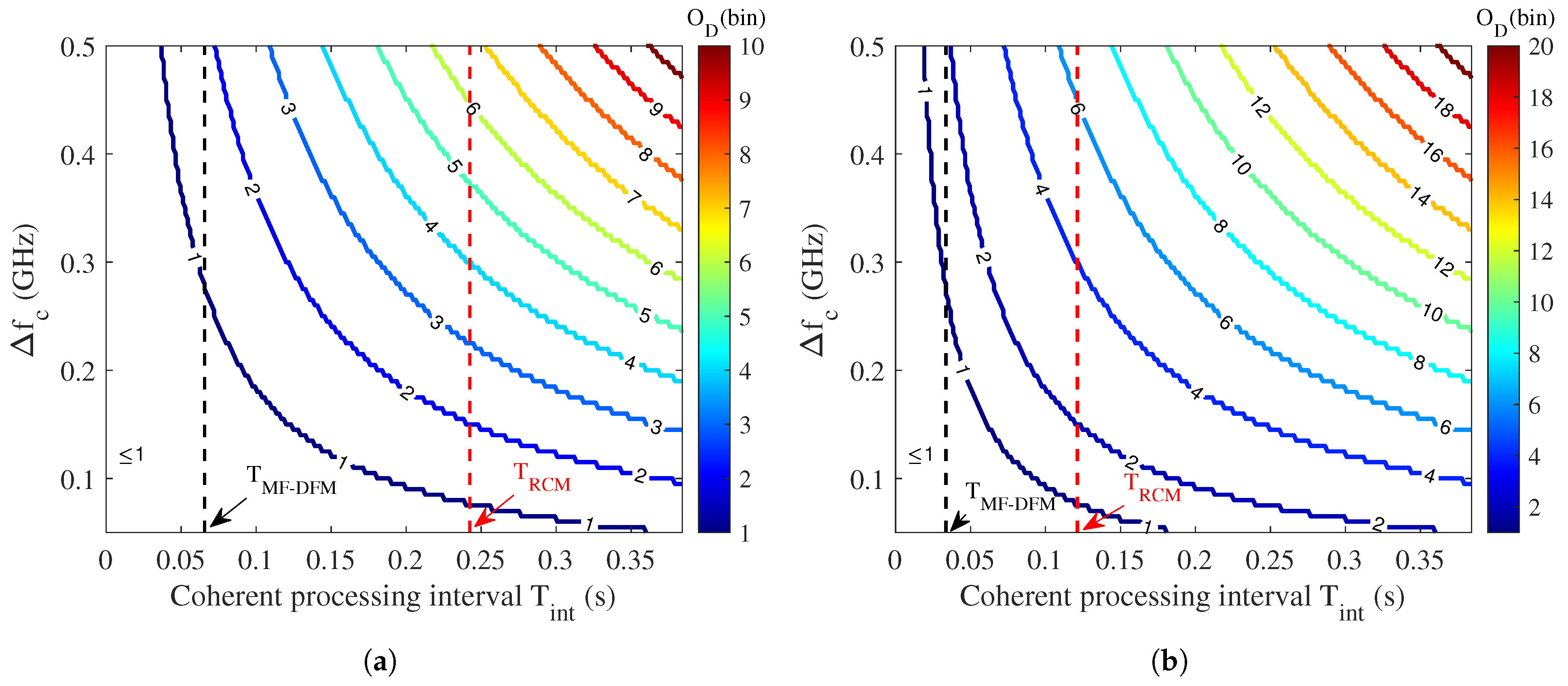
The main challenge of the DVB-S-based PBR is its extremely low power density on the Earth’s surface [18]. To cope with this limitation and achieve a robust detection of moving targets, long time integration and increasing the number of fusion channels are required to enhance the SNR of the weak echo. However, both of these will result in the energy misalignment [19], which can be divided into two parts: range cell migration (RCM) and Doppler frequency migration (DFM) [20]. Specifically, the target’s energy will disperse in multiple range cells due to the effect of RCM. Abundant solutions have been proposed to address the RCM, such as keystone transform (KT) [21], Hough transform (HT) [22], and their variants [23]. However, in the case of MFI, RCM occurs mainly due to the time-varying bandwidth, and RCM is particularly evident in FM-based PBR [9]. To circumvent this effect, a number of channels with consistent bandwidth are selected so that the target will locate in the same range bin at different frequency bands, due to the same physical path and range resolution. On the other hand, the conventional DFM is generated by the maneuverability (i.e., acceleration or jerk) of a moving target [20]. Typical methods for solving the DFM effect could be the phase matching (PM) approach [24], de-chirp method [25], chirp-Fourier transform [26], and fractional Fourier transform (FRFT) [27], etc.

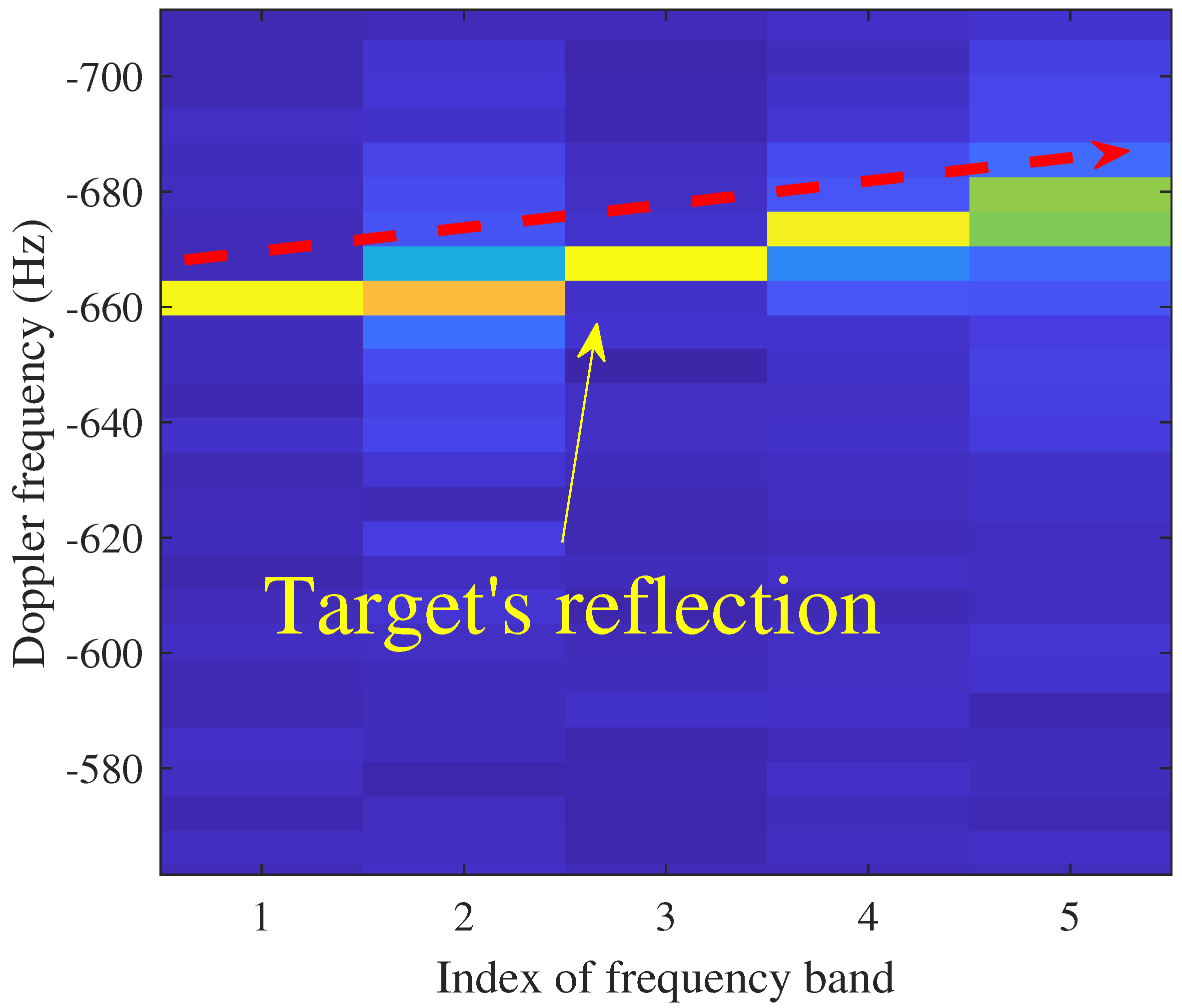
However, different from the conventional DFM, the DFM in MFI, called MF-DFM, imposes great challenges to MTD which need to be accounted for. According to [28], MF-DFM is caused by the frequency-hopping characteristic of the transmitted signal. If the same coherent processing interval (CPI) is employed in each frequency channel, the MF-DFM effect will result in the target appearing in different Doppler frequency bins, although the target moves with a constant velocity during the observations. Furthermore, when the radial velocity of the target is too high, or the CPI is too long, MF-DFM will become more evident, resulting in significant Doppler migration, which is also known as Doppler spread. This kind of migration cannot be eliminated by the conventional time–frequency method [28]. To address the MF-DFM, ref. [11] has proposed a practical solution, where different CPI in each frequency channel is allowed, thus enabling fusion with the same velocity resolution. Rather than fusion in range-Doppler mapping (RDM), ref. [11] performs fusion in the range–velocity mapping (RVM). However, there are two main limitations of using the approach in [11]. First, the CPI of each channel is specially selected, so it is non-trivial to generate multiple uniform RVMs for MF-based centralized detection. Interpolation or zero-padding is required at the cost of computational load. Second, ref. [11] combines multiple RVMs via non-coherent integration (NCI), which inevitably achieves less processing gain than the coherent ones.

Based on the principle of whether the phase information of the radar returns is used or not, the long-time integration methods can be divided into non-coherent integration and coherent integration. By exploiting the phase information, coherent integration can outperform non-coherent integration [29]. As an approach of coherent integration, Radon–Fourier transform (RFT) achieves moving target detection (MTD) with a long CPI [30,31]. Unlike the existing methods, RFT can be viewed as a generalized Doppler filter bank and processes signals jointly in the space–time–frequency domain [30]. Due to its outstanding performance, RFT and its variants have been extensively studied in various radar systems, such as offshore-based linear frequency-modulated (LFM) radar [32], and GNSS-based PBR [33,34]. However, thus far, there are limited studies that propose an RFT-based solution for migrating MF-DFM in MF-PBR. Moreover, RFT-based processing requires the nearly consistent phase of the target unit within the integration domain; otherwise, it will suffer from coherent integration loss if the standard deviation of the phase estimate exceeds a certain degree [35]. Consequently, it is imperative that the phase of the target in MF-RDMs should be estimated and compensated for prior to the coherent integration.

Motivated by the previous works, in this paper, we consider the quasi-coherent integration problem for MTD in MF-based PBR with an equal and long CPI in each frequency channel. According to our analysis, MF-DFM is likely to occur prior to the RCM, as the CPI increases. To focus on the issues in MF integration, including MF-DFM and residual phase errors, we primarily consider the detection scenario of a single point-like target with a constant velocity. The main contributions of this work are summarized as follows:

1.

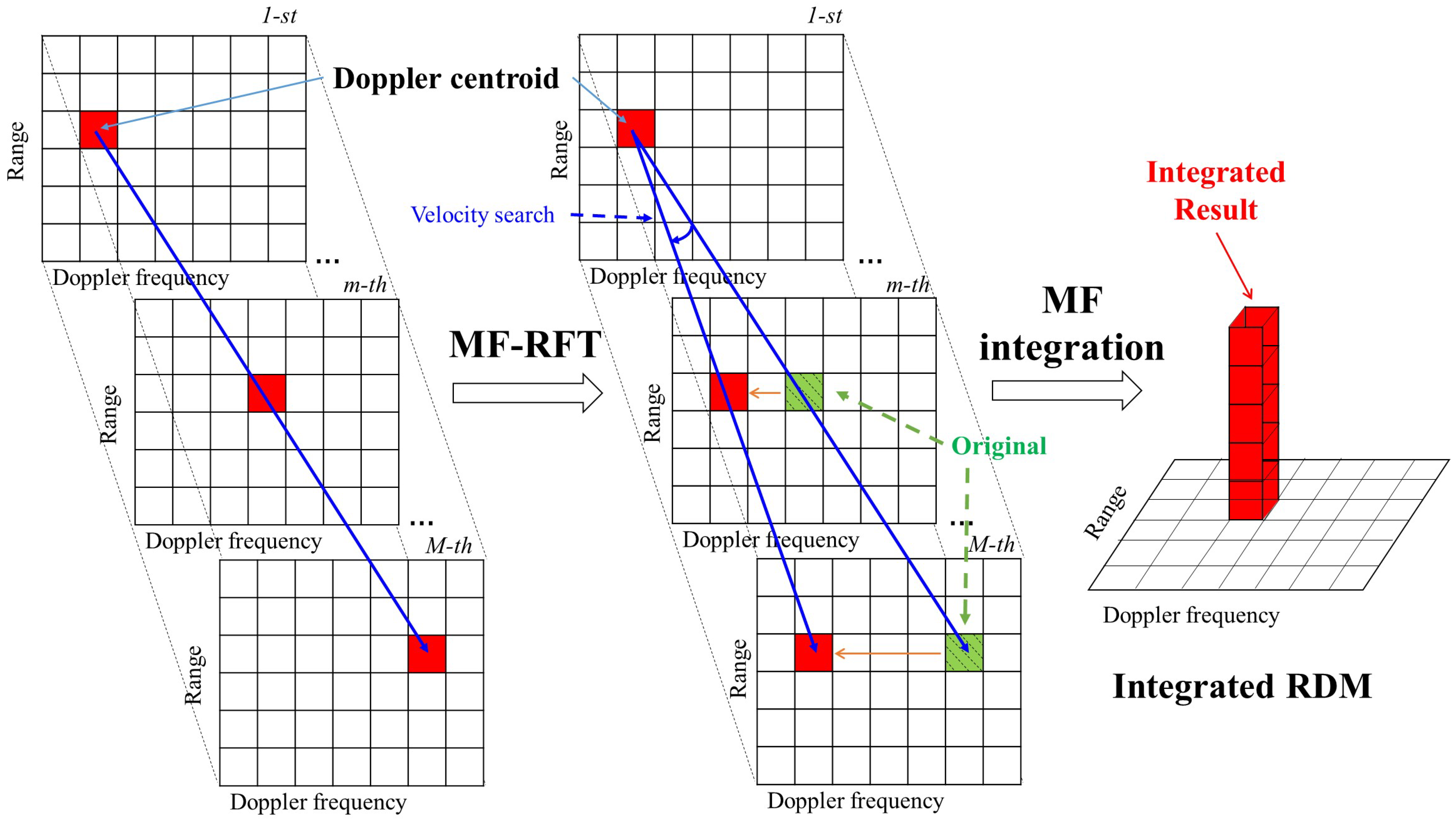
To eliminate the MF-DFM, a novel approach based on MF-based RFT (MF-RFT) is proposed. Specifically, a set of MF-Doppler filter banks (MF-DFBs) is dedicatedly designed, which is realized via conducting a thorough velocity search in the range/slow-time domain. By implementing this technique, the reflections of the moving target in the MF-RDMs can be focused on the Doppler centroid (DC) of the target, ultimately achieving the correction of the MF-DFM.

2.

To remove the residual phase errors following the MF-RFT, a phase-compensation-based method is also developed by formulating an optimization problem based on the minimum-entropy criterion. The particle swarm optimization (PSO) algorithm is then employed to solve the optimization problem for estimating the residual phase errors. Combining with MF-RFT, the proposed method could allow effective phase compensation, and quasi-coherent MF integration is then robustly achieved, improving the SNR of the weak target significantly.

Both simulated and field test results based on DVB-S signals show that the proposed algorithm could greatly improve the detection performance in the presence of MF-DFM and substantial residual phase errors, achieving better detection performance at low-SNR conditions, as compared with the existing algorithms.

The remainder of this article is organized as follows: Section 2 describes the signal model and the challenge in MFI, i.e., MF-DFM. The proposed method is then illustrated in Section 3. The effectiveness of the proposed algorithm is evaluated through simulation and field test results in Section 4. Finally, conclusions are drawn in Section 5.

2. Preliminary

2.1. Signal Model

Suppose that a quasi-monostatic MF-PBR system contains a reference channel (RC) and a surveillance channel (SC), as shown in Figure 1. The reference signal of the m-th frequency channel, i.e., $S_{ref,m}(t)$, is expressed as

$$S_{ref,m}(t)=b_m{s}_m(t)exp(j2\pi f_{m}t)+n_{ref,m}(t),m=1,2,\dots ,M,$$

(1)

where $b_m$ denotes the signal amplitude of the transmitted signal in the m-th RC, $f_m$ is the carrier frequency at the m-th frequency band, and $s_m(t)$ is the normalized communication signal emitted by IO in the m-th RC. Generally, $s_i(t)$ and $s_k(t)$ are uncorrelated for $i,k\in m$, $i\ne k$. $n_{ref,m}(t)$ is the noise in the m-th RC and it is assumed to be circularly symmetric and complex Gaussian noise with zero mean and variance of ${\sigma }_{r,m}^2$, i.e., $n_{ref,m}(t)\sim \mathcal{CN}(0,{\sigma }_{r,m}^2)$. M is the number of the frequency channel.

The surveillance signal in the m-th SC is expressed as

$$\begin{array}{c}{S}_{surv,m}(t)=c_m{s}_m(t)exp(j2\pi f_{m}t)+a_m{s}_m(t-{\tau }_m)exp(j2\pi f_{m}t)exp(j2\pi f_{d,m}t)+\\ n_{surv,m}(t),\hspace{1em}m=1,2,\dots ,M,\end{array}$$

(2)

where $c_m$ represents the signal amplitude for the propagation effect of the direct path interference (DPI) to the receiving antenna of the m-th SC. The symbols $a_m$, ${\tau }_m$, and $f_{d,m}$, respectively, denote the echo reflectivity, target delay, and Doppler frequency of the m-th SC. Without loss of generality, the reflected component in the m-th SC can be considered from the same target of interest. $n_{surv,m}(t)$ is the noise in the m-th SC and it is assumed to be circularly symmetric and complex Gaussian noise with zero mean and variance of ${\sigma }_{s,m}^2$, i.e., $n_{surv,m}(t)\sim \mathcal{CN}(0,{\sigma }_{s,m}^2)$. Generally, we assume that the noise in SC and that in RC are independently and identically distributed (IID).

Through a digital down-conversion (DDC) operation, the signals of RC and SC in the radio frequency (RF) band are converted to the baseband, and the problem of detecting the existence of a target is then formulated as a binary hypothesis, as follows:

$$\left\{\begin{array}{c}{H}_0:\left\{\begin{array}{c}{S}_{ref,m}(t)=b_m{s}_m(t)+n_{ref,m}(t),\hfill \\ S_{surv,m}(t)=c_m{s}_m(t)+n_{surv,m}(t),\hfill \end{array}\right.\hfill \\ H_1:\left\{\begin{array}{c}{S}_{ref,m}(t)=b_m{s}_m(t)+n_{ref,m}(t),\hfill \\ S_{surv,m}(t)=c_m{s}_m(t)+{\alpha }_m{s}_m(t-{\tau }_m)e^{j2\pi f_{d,m}t}+n_{surv,m}(t),\hfill \end{array}\right.\end{array}\right.$$

(3)

where $H_0$ and $H_1$ represent the absence and presence of the target of interest, respectively.

With the removal of DPI via the extensive cancellation algorithm (ECA) [36], the $c_m{s}_m(t)$ can be ignored in the following. As a result, the target problem in (3) is then modified as follows:

$$\left\{\begin{array}{c}{H}_0:\left\{\begin{array}{c}{S}_{ref,m}(t)=b_m{s}_m(t)+n_{ref,m}(t),\hfill \\ S_{surv,m}(t)=n_{surv,m}(t),\hfill \end{array}\right.\hfill \\ H_1:\left\{\begin{array}{c}{S}_{ref,m}(t)=b_m{s}_m(t)+n_{ref,m}(t),\hfill \\ S_{surv,m}(t)={\alpha }_m{s}_m(t-{\tau }_m)e^{j2\pi f_{d,m}t}+n_{surv,m}(t).\hfill \end{array}\right.\end{array}\right.$$

(4)

Next, we further discuss the target’s signatures, including ${\alpha }_m$, ${\tau }_m$, and $f_{d,m}$. Due to the same physical path and the consistent bandwidth at each selected frequency channel, the target delay at each frequency shows consistency, that is to say, ${\tau }_1=\dots ={\tau }_M$. However, the complex reflectivity ${\alpha }_m=a_{m}exp(j{\varphi }_m)$ could be different because of the fluctuated radar cross-section (RCS) at different frequency channels, especially for the target’s phase ${\varphi }_m$, resulting in substantial residual phase error. In addition, for the m-th channel, the target’s Doppler frequency is expressed as [37],

$$f_{d,m}=\frac{2V_{b}cos(\beta /2)}{{\lambda }_m}=\frac{g{f}_m{V}_b}{c},$$

(5)

where $V_b$ is the bistatic velocity of the target, $\beta$ is the bistatic angle, and g is geographical factor, which is equal to $2cos(\beta /2)$. Note that g can be absorbed by the bistatic velocity of the target $V_b$. Hence, there is no loss of generality to assume that $g=1$ ($\beta =120°$), and it can be ignored in the following derivation. As a result, the Doppler frequency of the moving target is coupled by the carrier frequency $f_m$ and the bistatic velocity of the target $V_b$. In general, the estimate of $f_{d,m}$ (i.e., ${\widehat{f}}_{d,m}$) via the conventional cross-ambiguous function (CAF) is completely different for different frequency bands if a long CPI is used [28].

2.2. The Challenges in MF Integration with a Long CPI

For a better understanding of the challenges in MF integration with a long CPI, we illustrate the importance of addressing the effects of MF-DFM by comparing the characteristics between RCM and MF-DFM. According to the analysis below, we will prove that the MF-DFM is likely to occur prior to RCM, as the CPI increases.

2.2.1. Rcm

RCM is a phenomenon occurring when the range resolution $\Delta R$ is high, as compared to the displacement of a target during the long-time integration. RCM causes the energy of the target echo to disperse in multiple range units, which reduces the processing gain of long-time integration. According to [20], RCM occurs when the following equation is satisfied,

$$\Delta R=\frac{c}{2Bcos(\beta /2)}<R(T_{int})-R(0),$$

(6)

where $R(T_{int})$ and $R(0)$ are, respectively, determined as follows,

$$R(T_{int})=R(0)+V_b{T}_{int}.$$

(7)

By substituting (7) into (6), we have,

$$\Delta R\le V_b{T}_{int}.$$

(8)

For avoiding RCM, the maximum value of the integration time is defined as,

$$T_{RCM}=\underset{T_{RCM}}{\mathrm{argmax}}\left[V_b{T}_{RCM}\le \frac{c}{2Bcos(\beta /2)}\right].$$

(9)

The above equation gives the upper bound for the appearance of RCM.

2.2.2. Mf-Dfm

In addition to RCM, MF-DFM is also an important phenomenon to be considered in MF-PBR. According to (5), the Doppler frequency of the target is proportional to the radial velocity $V_b$, and inversely proportional to the signal wavelength ${\lambda }_m$, i.e., proportional to the carrier frequency $f_m$. Meanwhile, the Doppler resolution of the radar system is inversely proportional to $T_{int}$, which indicates that the longer CPI is, the higher the Doppler resolution capability of the system, or the smaller the resolution unit $\Delta f_D$ will be. If sub-carrier segmentation is employed, the Doppler frequency of the target echo still changes as the carrier frequency of the RF signal, and the energy of the target will span multiple Doppler units when performing MF integration, i.e., MF-DFM, as shown in Figure 2. To better quantify this phenomenon, the factor of MF-DFM is defined as follows:

$$O_D=\frac{2\Delta f_c{V}_b{T}_{int}cos(\beta /2)}{c}.$$

(10)

The derivation of (10) is available in Appendix A, where $\Delta f_c$ = $f_M-f_1$ is the maximum separation of the carrier frequency. We can find that $O_D$ is proportional to $\Delta f_c$, $V_b$, and $T_{int}$. By fixing $V_b$ and $\Delta f_c$, $O_D$ increases as $T_{int}$ increases. If $O_D\ge 1$, then MF-DFM occurs as,

$$T_{int}\ge \frac{c}{2\Delta f_c{V}_{b}cos(\beta /2)}.$$

(11)

From (11), $T_{MF-DFM}$ is defined as follows:

$$T_{MF-DFM}=\underset{T_{MF-DFM}}{\mathrm{argmax}}\left[V_b{T}_{MF-DFM}\le \frac{c}{2\Delta f_{c}cos(\beta /2)}\right].$$

(12)

For the case of compact arrangement of MF, let $\Delta f_c=(M-1)B$. If $M\ge 2$, we have $\Delta f_c\ge B$. Compared with (9), we have,

$$T_{MF-DFM}\le T_{RCM}.$$

(13)

From the analysis above, we have proved that MF-DFM will appear prior to RCM as the integration time ($T_{int}$) increases. To simplify the problem and avoid the occurrence of both MF-DFM and RCM in the detection problem, we constrain $T_{int}$ between $T_{MF-DFM}$ and $T_{RCM}$, i.e., $T_{int}\in (T_{MF-DFM},T_{RCM}]$. This means the RCM can be avoided and the proposed algorithm aims to overcome the MF-DFM in MF integration.

For quantifying the $O_D$, Figure 3 shows the contour plots of $O_D$ with respect to the coherent integration time $T_{int}$, and the maximum separation of the carrier frequency $\Delta f_c$. The results are obtained by simulation according to Equation (10). The simulation settings are as follows: the range of CPI $T_{int}$ from 0.05 s to 0.36 s and $\Delta f_c$ from 0.05 GHz to 0.5 GHz. In addition, we temporarily ignore the geographical factor by setting $cos(\beta /2)$ = 1/2 ($\beta$ = 120°). Figure 3a,b give the contour plots when $V_b$ equals 60 km/h and 120 km/h, respectively. We can see that $O_D$ increases as $T_{int}$, $V_b$, and $\Delta f_c$ increase. The value of $O_D$ indicates the extent of MF-DFM. For example, when $\Delta f_c$ = 0.3 GHz, $T_{int}$ = 0.2 s, and $V_b$ = 60 km/h, $O_D$ is equal to 3.1, which means that the Doppler shift of the target will spread to more than 3 consecutive Doppler units. For a better understanding of the meaning of CPI, the time limit of RCM, i.e., $T_{RCM}$, is also plotted in Figure 3. The time limit of MF-DFM ($O_D$ = 1) is determined according to the value of the $\Delta f_c$ and $V_b$. Figure 3 also gives the time limit of MF-DFM when $\Delta f_c$ = 0.28 GHz (12.675 GHz − 12.395 GHz).

It is noted that only MF-DFM in the MFI is discussed above. However, a more comprehensive case will occur with both RCM and MF-DFM when the CPI continues to increase. Thanks to the existing techniques of KT, the RCM can be effectively solved. In addition, the detection problem with MFI will become extremely complicated if a target with high maneuverability and high speed is considered. More efforts should be performed for the cases where the target is maneuverable, of high speed, and even extended. To focus on the issues in MF integration, including MF-DFM and residual phase errors, we primarily consider the detection scenario of a single point-like target with a constant velocity.

3. Proposed Algorithm

To overcome MF-DFM, we propose an MF-based RFT (MF-RFT) algorithm, which can be viewed as an extension of RFT in the multi-frequency domain. Specifically, to implement MF-RFT, we first design a set of MF-based DFB (MF-DFB), which can correct the MF-DFM of the target in the MF domain and enables the reflected energy to focus in the DC of the target. Then, in order to realize the quasi-coherent MF integration, an optimization problem for phase estimation is formulated based on the minimum-entropy criterion. Then, the PSO algorithm is employed to solve the optimization problem. Finally, the SNR of the target echo is greatly improved using MF synthesis. In the following, we investigate them accordingly.

3.1. Definition of MF-RFT

According to [30], RFT achieves coherent integration of the target’s energy via DFB obtained by searching motion parameters. As an extension of RFT, MF-RFT enables the elimination of the MF-DFM effect by designing a sequence of MF-DFB. The derivation of MF-DFB is given in the following.

From (2), we define the Doppler term of the target, $K_m=exp(j2\pi f_{d,m}t)$. By substituting (5) into $K_m$, $K_m$ can be rewritten as follows:

$$\begin{array}{cc}\hfill K_m=& exp\left(\frac{j2\pi f_m{V}_{b}t}{c}\right)\hfill \\ \hfill =& exp\left[\frac{j2\pi (f_1+f_m-f_1)V_{b}t}{c}\right]\hfill \\ \hfill =& exp(j2\pi f_{d,1}t)H_m,\hfill \end{array}$$

(14)

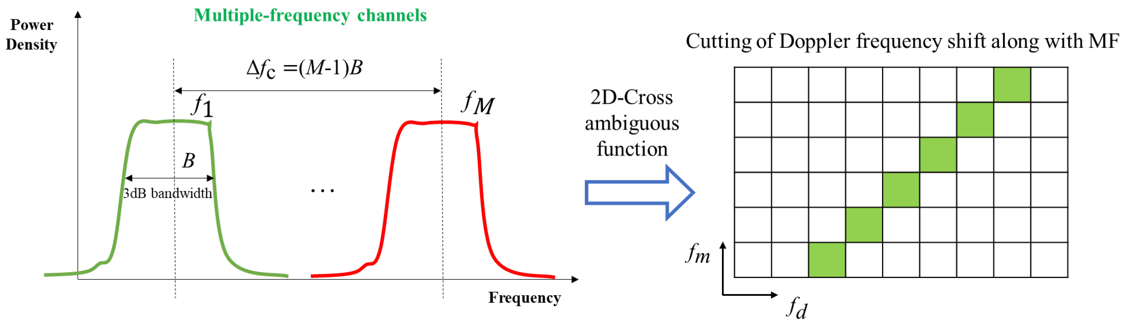
where $f_{d,1}=f_1{V}_b/c$, is the Doppler centroid of the moving target, as shown in Figure 4. As consequently, the coefficients of MF-DFB are defined as follows:

$$H_m(V_b)=exp\left[\frac{j2\pi (f_m-f_1)V_{b}t}{c}\right]$$

(15)

Obviously, given a set of selected frequency channels, i.e., $\overrightarrow{f}=[f_1,\dots ,f_M]$, and a velocity of interest $V_b$, the coefficients of $H_m$ are uniquely determined. In other words, leveraging the prior knowledge of the carrier frequency can effectively reduce the computational burden of the MF-DFB. In practice, the target’s velocity is usually unknown. However, it is possible to employ a velocity search to estimate the target’s velocity. This means the coherent synthesis of multiple RDMs, i.e., $I_{MF}(r,f_d)$, reaches its maximum only when the searching parameter matches the true target’s velocity $V_b^{*}$, i.e., $V_b=V_b^{*}$. The coherent synthesis of multiple RDMs, i.e., $I_{MF}(r,f_d)$, is defined as follows:

$$I_{MF}(r,f_d;V_b)={\left|\sum _{m=1}^M{I}_{MF-DFB,m}(r,f_d;V_b)\right|}^2,$$

(16)

where $I_{MF-DFB,m}(r,f_d;V_b)$ is the m-th filtered RDM, which is calculated as,

$$I_{MF-DFB,m}(r,f_d;V_b)={\int }_{-{\eta }_K/2}^{{\eta }_K/2}{R}_m(r,{\eta }_k)H_m(V_b)exp(-j\frac{2\pi f_{d}k{\eta }_k}{K})d{\eta }_k,$$

(17)

where $R_m(r,{\eta }_k)$ is the two-dimensional (2-D) matrix obtained by batch-based range compression and stacking along slow-time. ${\eta }_k$ is the index of slow-time. As a result, the Doppler frequencies of the target in the m-th frequency band can be corrected to the DC of the target because of the MF-DFB.

To implement the calculation of (17), discrete Fourier transform (DFT) can be employed. Accordingly, Equation (17) can be rewritten as follows:

$$I_{MF-DFB,m}(r,f_d;V_b)=DF{T}_{\eta }[R_m(r,{\eta }_k)H_m(V_b)],\hspace{1em}k=1,2,\dots ,K$$

(18)

where $DF{T}_{\eta }$ denotes the DFT along the slow-time dimension. As a result, the estimation of the unknown target’s velocity is obtained by solving the following optimization problem as follows:

$$\begin{array}{c}\hfill {\widehat{V}}_b=\underset{r,V_b}{argmax}\left[{\left|\sum _{m=1}^{M}DF{T}_{\eta }[R_m(r,\eta )H_m(V_b)]\right|}^2\right],\\ \hfill r\in [r_{min},r_{max}],\hspace{1em}\hspace{1em}{V}_b\in [V_{b,min},V_{b,max}].\end{array}$$

(19)

The above optimization problem can be solved by first fixing a small region of interest (ROI) r and then performing a parameter search of $V_b$.

As shown in Figure 4, the filter coefficients of MF-DFB are then be determined after the velocity search. The final output of MF-RFT is expressed as follows:

$$T_{MF-RFT}(r,f_d)={\left|\sum _{m=1}^{M}DF{T}_{\eta }[R_m(r,{\eta }_k)H_m({\widehat{V}}_b)\right|}^2.$$

(20)

Using (20), the MF-DFM effect can be eliminated by the proposed MF-RFT so that the target envelope can be locked in the same Doppler cell. However, the derivation above ignores the residual phase error in the target unit. The residual phase error will lead to coherent integration loss. In [35], the authors have shown that the coherent integration loss depends on the distribution of the phase error. In the case of a uniform distribution, the coherent integration loss will exceed 2 dB when the standard deviation of the phase fluctuation exceeds 0.7 rad, and will reach 5 dB when the standard deviation of the phase exceeds 1 rad.

If the phase information in MF is unknown or difficult to compensate for, the NCI-based MF-RFT (MF-RFT-NCI) is a practical choice. The velocity search in MF-RFT-NCI is modified as follows:

$$\begin{array}{c}\hfill {\widehat{V}}_{b,NCI}=\underset{r,V_b}{argmax}\left[\sum _{m=1}^M{\left|DF{T}_{\eta }[R_m(r,\eta )H_m(V_b)]\right|}^2\right],\\ \hfill r\in [r_{min},r_{max}],\hspace{1em}\hspace{1em}{V}_b\in [V_{b,min},V_{b,max}].\end{array}$$

(21)

Note that (21) is quite different from (19), since (21) employs a squared magnitude operation and NCI-based summation, while (20) performs coherent summation and then squares the magnitude. Phase synchronization is needed in MF-RFT. Accordingly, the MF-RFT-NCI can be obtained as

$$T_{MF-RFT-NCI}(r,f_d)=\sum _{m=1}^M{\left|DF{T}_{\eta }[R_m(r,{\eta }_k)H_m({\widehat{V}}_{b,NCI})]\right|}^2.$$

(22)

Based on the NCI-based processing, the final detection results are achieved by the generalized gamma-based constant false alarm rate (CFAR) detector [38].

3.2. Me-Based PSO Algorithm for Phase Estimation

The processing gain of NCI-based processing is limited as compared with coherent processing. In the following, an ME-based phase estimation method is proposed to eliminate the effect of the residual phase error. In order to ensure the availability of coherence, it is intuitive to estimate and compensate for the residual phase for further improving the processing gain of MF-RFT processing.

Given a certain range and velocity, i.e., r and $V_b$, the output of MF-DFB with phase compensation can be expressed as,

$$S_m(f_d,{\varphi }_m;r,V_b)=DF{T}_{\eta }[R_m(r,{\eta }_k)H_m(V_b)exp(-j{\varphi }_m)],\hspace{1em}{\varphi }_m\in [0,2\pi ],$$

(23)

where ${\varphi }_m$ is utilized to cancel the phase error. To determine ${\varphi }_m$, we formulate it as an optimization problem based on the global minimum-entropy criterion [39], as follows:

$$E({\varphi }_m;r,V_b)=-\frac{1}{Dim(f_d)}\sum _{f_d}\left[\frac{|{\sum }_{m=1}^M{S}_m(f_d,{\varphi }_m){|}^2}{C}ln\frac{|{\sum }_{m=1}^M{S}_m(f_d,{\varphi }_m){|}^2}{C}\right]$$

(24)

where $Dim(f_d)$ is the dimension of the Doppler domain, and C is a normalized term, which is calculated as,

$$C=\sum _{f_d}{\left|\sum _{m=1}^M{S}_m(f_d,{\varphi }_m;r,V_b)\right|}^2.$$

(25)

Consequently, finding ${\varphi }_m$ can be achieved by minimizing the optimization problem as,

$$\begin{array}{c}\hfill {\varphi }_m=\underset{{\varphi }_m}{argmin}[E({\varphi }_m;r,V_b)],\\ \hfill 0<{\varphi }_m\le 2\pi ,m=1,\dots ,M.\end{array}$$

(26)

To ensure the uniqueness of the solution, we usually constrain ${\varphi }_1$ = 0. The above optimization problem is high-dimensional and nonlinear, so it is non-trivial and NP-hard to prove its convexity. In the case when M is small, exhausted searching (ES) can be used to obtain the optimal minimum of (26). However, in practical conditions, ES is not a desirable choice since its computational complexity increases with the exponential of M, i.e., $O(N^M)$. As a greedy algorithm, the dynamic program (DP) can solve the above optimization problem with a lower computational complexity but DP cannot guarantee the global optimal when the SNR is extremely low. To reduce the complexity of the algorithm as well as guaranteeing the optimality of the solution, we choose the PSO algorithm in [40] to solve (26). Compared with ES, PSO is an efficient algorithm that can converge within a certain number of iterations and achieves satisfactory accuracy, although the result is not necessarily the optimum.

The parameter notation in the ME-based PSO (ME-PSO) algorithm is summarized as follows:

1.

$N_p$: The population of particles which is initialized, and i is its subscript index;

2.

M: The dimension of the particles’ state, which is the same as the number of the used fusion channel;

3.

$k_{max}$: The maximum number of iterations; k is the iteration index;

4.

${\Phi }_i^k\in R^{M\times 1}$: The phase vectors of the i-th particle at the k-th iteration, where R is denoted as fields of a real number;

5.

${\mathbf{V}}_i^k\in R^{M\times 1}$: The velocity vectors of the i-th particle at the k-th iteration;

6.

w: The inertia weights, which are used to control global exploration and local exploration of the particles;

7.

$c_1,c_2$: The two independent and uniformly distributed random numbers accounting for random movements of the particle. In experiments, we generally set $c_1$ = 0.5 and $c_2$ = 0.5. $r_1$ and $r_2$ are random numbers with intervals of [0,1], denoted by rand ([0,1]);

8.

${\mathbf{pbest}}_i^k\in R^{M\times 1}$: The personal best of the i-th particle at the k-th iteration;

9.

${\mathbf{gbest}}^k\in R^{M\times 1}$: The global best at the k-th iteration.

The procedures of the proposed ME-based PSO algorithm for phase estimation is shown in Algorithm 1.

Algorithm 1: ME-based PSO for phase estimation
	Input: Intial phase vectors ${\{{\Phi }_i^0\}}_{i=1}^{N_p}$ (also known as the initial state of the particles), inital velocity vectors of the particles ${\{{\mathbf{V}}_i\}}_{i=1}^{N_p}$, maximum loop times $k_{max}$, and $S_m(f_d,{\varphi }_m;r,V_b)$, for $m=1,2,\dots M$.
	Output: Optimal/suboptimal phase estimation ${\Phi }^{*}$.
1	Initialize the random parameters, including $w=0.8$, $c_1=0.5$, and $c_2=0.5$, $k=1$, ${\mathbf{pbest}}_i^0={\Phi }_i^0$, ${\mathbf{gbest}}^0=\underset{{\Phi }_i^0}{argmin}E{({\Phi }_i^0)}_{i=1}^{N_p}$, where fitness value $E()$ using (24).
2	while $k\le k_{max}$ do
3				for $i=1,2,\dots ,N_p$ do
4						$r_1$ = rand([0, 1]), $r_2$ = rand([0, 1]),
5						${\mathbf{V}}_i^k=w{\mathbf{V}}_i^{k-1}+c_1{r}_1({\mathbf{pbest}}_i^{k-1}-{\Phi }_i^{k-1})+c_2{r}_2({\mathbf{gbest}}^{k-1}-{\Phi }_i^{k-1})$,
6						${\Phi }_i^k={\Phi }_i^{k-1}+{\mathbf{V}}_i^k$;
7						if and else;
8						if $E({\mathbf{pbest}}_i^{k-1})<E({\Phi }_i^k)$ then
9							${\mathbf{pbest}}_i^k={\Phi }_i^k$;
10						else
11							${\mathbf{pbest}}_i^k={\mathbf{pbest}}_i^{k-1}$;
12						end
13						if and else;
14						if $E({\mathbf{gbest}}^{k-1})<E({\Phi }_i^k)$ then
15							${\mathbf{gbest}}^k={\Phi }_i^k$;
16						else
17							${\mathbf{gbest}}^k={\mathbf{gbest}}^{k-1}$;
18						end
19				end
20				${\Phi }^{*}={\mathbf{gbest}}^k$, $k=k+1$;
21	end

3.3. Phase Compensation and MF Quasi-Coherent Integration

After the MF-RFT and ME-PSO-based phase estimation, the phase compensation should be performed for quasi-coherent MF integration. Since the signatures of the target are unknown, phase compensation cannot accurately be performed only to the target’s unit. Instead, phase compensation is required to be performed in each range-Doppler cell as,

$$T_{MF-RFT-QCI}(r,f_d)={\left|\sum _{m=1}^{M}DF{T}_{\eta }[R_m(r,{\eta }_k)H_m({\widehat{V}}_b)exp(-j{\widehat{\varphi }}_{ME-PSO,m})\right|}^2.$$

(27)

The combination of MF-RFT and ME-PSO can be categorized as a quasi-coherent detector [41], and thus it is denoted by MF-RFT-QCI for simplicity of notation. Using (27), a target peak will be generated on the integrated RDM by simultaneously correcting the MF-DFM and the residual phase error. To confirm whether the target peak is the detected target or not, the biparametric CFAR detector employed in [42] can form the Gaussian distributed test statistic using vast IID samples.

3.4. Implementation of the Proposed Algorithm

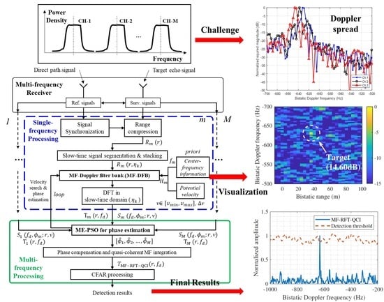
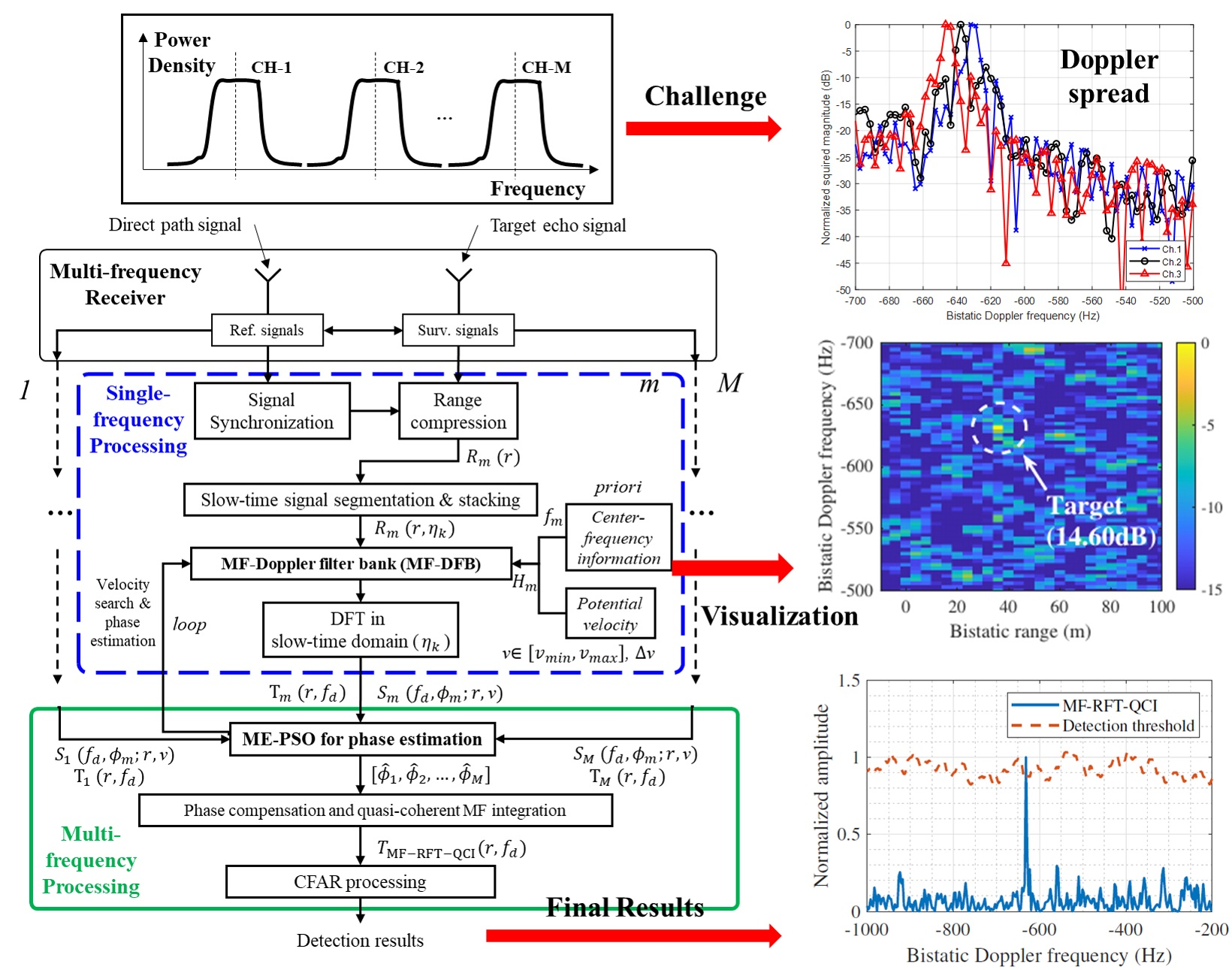
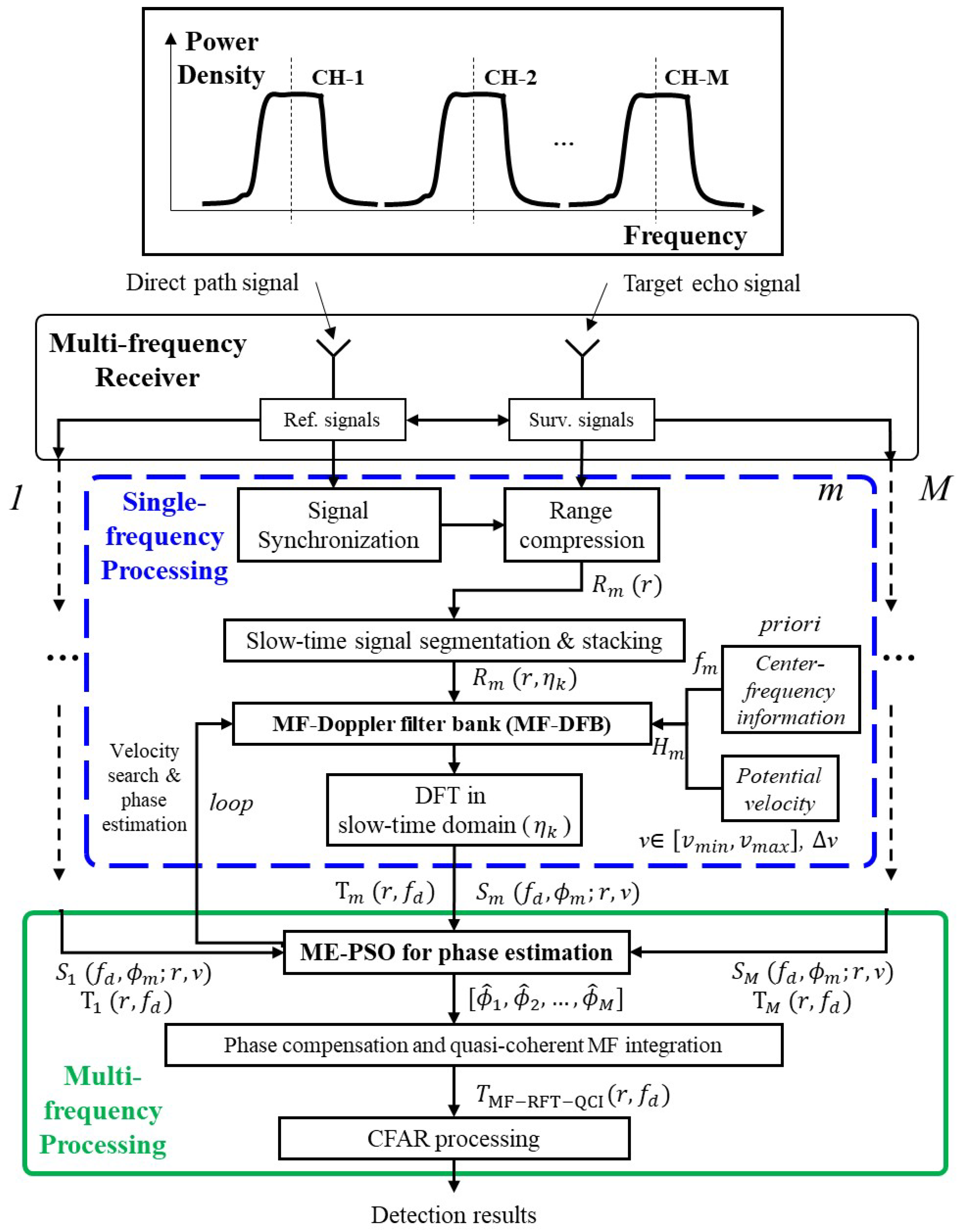
For a better understanding of the proposed algorithm, Figure 5 gives the flowchart of the proposed algorithm, which consists of seven steps. The procedures of the proposed algorithm are illustrated step-by-step in the following.

Step 1: Carry out the demodulation and batch-based range compression to accumulate energy within each frequency channel.

Based on the MF coherent PBR receiver, the target returns are sampled in fast-time in the intermediate frequency (IF). Then, the sample data are digitally down-converted (DDC) into the signal of the baseband, which is also known as demodulation. With the use of corresponding signals of RC, the batch-based range compression [43] is used for the first stage of coherent integration in the fast-time domain. The data, after batch-based range compression, are stored as a 2-D matrix in the range and slow-time domains, i.e., $R_m(r,{\eta }_k)\in C^{N/K\times K}$, for $m=1,\dots ,M$, $k=1,2,\dots ,K$. The signals at different frequency bands are also processed in parallel.

Step 2: Parameter initialization for MF-RFT and ME-PSO algorithm.

First, parameter initialization for the MF-RFT algorithm is given as follows: the coherent integration time $T_{int}$, the number of batches in slow-time K, the range search scope $[r_{min},r_{max}]$. Based on the relative prior information such as moving statues of the target to be detected, the expected search scope of the velocity $[V_{min},V_{max}]$, and the velocity interval $\Delta V_b$ is defined as,

$$\Delta V_b=\frac{c}{2f_{c,1}{T}_{int}}$$

(28)

Therefore, the values of the search range are $N_r$ = round[($r_{max}-r_{min}$)/$\Delta r$], where $\Delta r$ denotes the range resolution as (6), and round[] denotes the operation of rounding up to an integer. Similarly, the search value of the velocity is $N_v$ = round[($V_{b,max}-V_{b,min}$)/$\Delta V_b$]. In particular, the coherent integration time $T_{int}$ should be specially selected, i.e., $T_{int}\in (T_{MF-DFM},T_{RCM}]$ for avoiding the RCM.

Second, the parameter initialization of the ME-PSO algorithm is given as follows: According to [44], the population of the particles $N_p$ is set as 80. Most importantly, the particles ${\Phi }_m$ are initialized randomly and as uniformly distributed in the searching space as possible. The maximum iteration $k_{max}=50$.

Step 3: Apply the MF-RFT to eliminate the MF-DFM using a velocity search.

Given a search range r, this step is performing the MF-DFB to estimate the target’s velocity $V_b$. Given the prior knowledge of the carrier frequency, the expected search scope of the velocity $[V_{min},V_{max}]$, and velocity interval $\Delta V_b$, and the coefficients of MF-DFB, i.e., $H_m(V_b)$ can be determined using (15).

Step 4: Perform PSO algorithm for phase estimation.

Given a searching velocity $V_b$, this step is to find the estimate of the residual phase error by solving the optimization problem in (26). It is noted that the accuracy of phase estimation is highly related to the dimension of the searching space of the range and Doppler frequency. To the best knowledge of the authors, the interesting range is as limited as possible.

Step 5: Go through all the searching parameters and obtain the estimates of the unknown parameters.

Go through all the searching scope of range, velocity, and phase. Repeat steps 3 and 4 to obtain a peak value in the range-Doppler domain, as

$$(r^{*},V_b^{*},{\varphi }_m^{*})=\underset{r,V_b,{\varphi }_m}{argmax} T_{MF-RFT-QCI}$$

(29)

where $T_{MF-RFT-QCI}$ is calculated as (27).

Step 6: Perform quasi-coherent integration and construct the integrated RDM.

With the estimation of range, velocity, and phase, the integrated RDM can be obtained using (27). It is noted that the above operations will lead to power deviation, so a normalization in MF is required before quasi-coherent MF integration.

Step 7: Carry out the CFAR detection to confirm a target.

Take the squared magnitude of the integrated RDM in step 6 as the test statistic, and compare it with the adaptive threshold for a given expected false alarm rate as,

$$T_{MF-RFT-QCI}(r,f_d)\begin{array}{c}{H}_1\\ \gtrless \\ H_0\end{array}\gamma ,$$

(30)

where $\gamma$ is the adaptive threshold obtained by the CFAR detector. If the test statistic is smaller than the threshold, there will be no moving target detected. The CFAR process goes through all the cells under test (CUTs) and yields the final detection results.

3.5. Consideration of Computational Complexity

Although the proposed method is reasonably superior to the existing methods in terms of detection capability via migrating MF-DFM and residual phase errors, the improved performance comes at the cost of computational complexity. Specifically, the increased complexity comes from several aspects: (1) the range search; (2) the velocity search in MF-DFB; and (3) the phase estimation by the ME-PSO algorithm. Fortunately, when the parameters of the radar system are given and some prior information (such as location) of the target to be detected can be obtained, the searching area in the parameter space can be greatly reduced [32]. Specifically, the location information can be obtained from the previous tracking records or high-SNR results. The location information is not necessarily accurate before detection since the range search in the proposed MF-RFT can refine the location based on the coarse location information and reduce the scope of the range search, which also results in a decreased computational load. On the contrary, the scope of the range search should be extended to the maximum detection range of the target if the location information of the target is unavailable [45]. In addition, many operations, such as MF-DFB, can be replaced by the fast Fourier transform (FFT) algorithm if the number of Doppler dimensions is an integer power of two. Moreover, the proposed ME-PSO algorithm for phase estimation can significantly alleviate the computational burden with acceptable performance. Therefore, the proposed approach is promising for real-world implementation, and its running time will be evaluated in the next section.

4. Performance Evaluation

In this section, the effectiveness of the proposed method is verified using numerical results and field test results, respectively. For the field test, the experiment is carried out using the self-developed multi-channel passive radar (McPR) system based on the DVB-S signal.

4.1. Numerical Results

The numerical results can be divided in two parts. First, the effectiveness of the proposed algorithm is verified using a case study. Second, the detection performance of the proposed algorithm is then evaluated using Monte Carlo simulations.

To effectively quantify the performance, we, respectively, specify the SNR of the RC and the SNR of the SC at the m-th frequency band as:

$$\begin{array}{c}\hfill SN{R}_{RC,m}=\frac{|b_m{|}^2}{{\sigma }_{r,m}^2},\end{array}$$

(31)

$$\begin{array}{c}\hfill SN{R}_{SC,m}=\frac{|{\alpha }_m{|}^2}{{\sigma }_{s,m}^2},\end{array}$$

(32)

where the definitions of $b_m$, ${\alpha }_m$, ${\sigma }_{r,m}^2$, and ${\sigma }_{s,m}^2$ can be found in (1) and (2).

4.1.1. Case Study

For verifying the effectiveness of the proposed method, we provide a case study, where the simulated parameters are set as follows. First, the channel occupation is based on the investigation of the IOs that emit the DVB-S signal. Among the investigated IOs, the Apstar-6C is chosen since it can provide multiple adjacent frequency channels with the same bandwidth and polarization [46]. Actually, the DVB-S standard transmits multi-frequency signals via a single carrier per transponder with time division multiplex (TDM) or multi-carrier frequency division multiplex (FDM) [47]. Apstar-6C employs the latter, and as a result, the concern about illuminating the target asynchronously can be ignored in this case. In the radar system using the Apstar-6C as the IO, the channel number for fusion $M=5$, the carrier frequencies range from 12.395 GHz to 12.675 GHz, the sample rate $f_s$ = 100 MHz, and the signal bandwidth $B=36$ MHz. The noise in different frequency bands is assumed to be IID. We consider a case, where a target is moving with a constant speed and distance of 16 m/s and 40 m, respectively. For avoiding the RCM, the CPI $T_{int}$ for each channel is selected as 0.1678 s. As a result, the processing gain $G_p$ = 10 × log₁₀(B × $T_{int}$) = 71.23 dB. The simulation settings are summarized in

Table 1. Simulation settings for case study.

Parameter	Value	Parameter	Value
Freq. of Ch. 1	12.395 GHz	Sample rate	100 MHz
Freq. of Ch. 2	12.435 GHz	Bandwidth	36 MHz
Freq. of Ch. 3	12.515 GHz	Modulation	QPSK
Freq. of Ch. 4	12.595 GHz	Target’s velocity	−16 m/s
Freq. of Ch. 5	12.675 GHz	Target’s range	40 m
CPI	0.1678 s	Input SNR${}_{SC}$/SNR${}_{RC}$	−63/10 dB
Range resolution	4.04 m	Doppler frequency resolution	5.96 Hz

.

According to the simulation settings, the largest separation of the carrier frequency is 280 MHz (i.e., $f_{c,5}-f_{c,1}$), the Doppler frequency resolution and range resolution of the system are 5.96 Hz and 4.04 m, respectively. During the observation time of 0.1678 s, the displacement of the target is 2.6848 m, which does not exceed the range resolution. Consequently, RCM does not occur. However, according to (10), the variation in the target’s Doppler frequency ranges from −660 Hz to −680 Hz at different frequency bands. Consequently, the target’s energy will disperse in up to three sequential Doppler cells. This Doppler spread will be further intensified as the CPI and channel number continue to increase. For confirming the analysis above, the MF-DFM of the moving target is shown in Figure 6, where it is noise free.

The performance comparison of different methods is given in Figure 7, where a three-dimensional (3D) RDM is provided. For the sake of comparison, this case only focuses on the migration of MF-DFM, so the residual phase error is temporarily not considered. For a comprehensive comparison, the MF-NCI with equal-length CPI (MF-NCI-EL) [48], MF-NCI with unequal-length CPI (MF-NCI-UEL) in [11], and MF-RFT-NCI in (22) are selected. For a fair comparison, the CPIs at each frequency channel in MF-NCI-UEL are specially selected and their total CPI is the same as that in the other detectors (i.e., $M\times T_{int}$). The input $SN{R}_{SC,m}$, are all set as −60 dB. From Figure 7a–d, one can observe that the output SNR from MF-NCI-EL is the worst due to its lack of Doppler spread correction. Therefore, the target’s energy cannot be concentrated in the same Doppler frequency bin, and the weak target is submerged below the noise floor, as shown in Figure 7a. From Figure 7b, the MF-DFM can be alleviated via MF-NCI-UEL but the output SNR is minor due to the non-ideal range misalignment. Consequently, the faint target also cannot be effectively detected by the subsequent CFAR detector. On the contrary, better performance can be achieved by MF-RFT-NCI, as shown in Figure 7c. Although it does not exploit the phase information, the target’s energy can be effectively enhanced due to the MF-DFB in the non-coherent mode by (21). From Figure 7d, the output SNR of the proposed MF-RFT-QCI is the highest among the considered methods, since it benefits from both MF-DFB in the coherent mode and the exploitation of phase information of the target. These results confirm the effectiveness of the proposed method in the detection scenarios with MF-DFM.

Next, the effectiveness of the proposed ME-PSO algorithm for phase compensation is also evaluated. The comparison of the Doppler profile of MF-RFT with and without the ME-PSO algorithm is shown in Figure 8. Herein, we consider a case when M = 3 ($[f_1,f_2,f_3]$ = [12.395, 12.515, 12.675] GHz) and the other settings are the same as in Figure 7. The phase of the target at different frequency bands $[{\varphi }_1,{\varphi }_2,{\varphi }_3]$ are equal to 1.487, 0.593, and −2.080 (in radian), respectively. The standard deviation of the target’s phase exceeds 1.85 radians. From Figure 8, the output SNR of MF-RFT with ME-PSO is significantly better than that of MF-RFT without ME-PSO in this case. This result verifies the effectiveness of the proposed phase estimation method and the importance of the phase compensation in quasi-coherent MF integration in the presence of substantial residual phase error.

4.1.2. Detection Performance

Detection Performance in the Presence of MF-DFM

In this section, the detection performance of the proposed algorithm is evaluated using Monte Carlo simulations. Assuming that the input SNR of the target echo varies from −70 dB to −60 dB, the output SNR of the target echo is obtained using different fusion methods, including the conventional MF-NCI-EL, MF-NCI-UEL, MF-RFT-NCI, and the proposed MF-RFT. Meanwhile, the results are obtained via 100 Monte Carlo simulations. For controlling the false alarms, the expected false alarm probability $P_{fa}$ in the CFAR detector is set to ${10}^{-5}$. In the CFAR detector, the total number of the training cells in range and Doppler axis Q = 60, and the shape of the guard cell is set to a rectangular window with a size of 5 × 5. In this setting, the CFAR loss is limited below 0.2 dB.

Figure 9a shows the detection probability as a function of the input $SN{R}_{SC}$ when only the MF-DFM is considered. From Figure 9a, the proposed method can obtain, respectively, 1.2 dB, 1.5 dB, and 5 dB of SNR improvement for the detection probability of 0.9, with the MF-RFT-NCI, MF-NCI-UEL, and MF-NCI-EL. These results further confirm the effectiveness of the MF-DFB for migrating MF-DFM.

Reaching a constant false alarm and maximum detection probability condition in a PBR system is quite important. To verify the CFAR property of the considered methods, Figure 9b shows the measured $P_{fa}$ as a function of different input $SN{R}_{SC}$. The measured $P_{fa}$ is defined as,

$$\mathrm{Measured} P_{fa}=\frac{FAR}{N_R{N}_D},$$

(33)

where $FAR$ is the number of false alarms generated by the CFAR detector in the observation region, and $N_R{N}_D$ is the total number of range-Doppler resolution units. This result indicates that the measured $P_{fa}$ is consistent with the expected one, showing the capability of controlling $P_{fa}$. Moreover, this result also verifies the fairness of the comparison of different fusion detectors in terms of detection probability in Figure 9a.

Robust Detection Performance against Residual Phase Error

Next, we further evaluate the detection performance of the proposed method in the presence of the residual phase error. Note that, in order to limit the computational burden, in this subsection, we set M = 3, and the selected carrier frequencies are 12.395, 12.515, and 12.675 GHz, respectively. The residual phase error is modeled as the uniform distribution [35], i.e., ${\varphi }_m\sim U[0,p]$, where $0<p\le 2\pi$ denotes the fluctuation in phase error. In addition, p and M, the other simulation settings, are the same as in the previous simulation. For a better understanding of the effectiveness of the PSO-based algorithm, we select the MF-RFT without PSO-based phase estimation for comparison. The detection performance of the consider detector under different p is given in Figure 10, where $p=\pi /2,\pi$, and $2\pi$ are shown in Figure 10, respectively. From the results, we can conclude that the performance of the proposed MF-RFT-QCI is robust to the residual phase error, while the performance of the MF-RFT without ME-PSO drops significantly as the fluctuations in the residual phase error p increase. For achieving a PD of 90%, the proposed MF-RFT with ME-PSO can, respectively, achieve approx. 3.9 dB and 9.4 dB of processing gain over the MF-RFT without ME-PSO when p = $\pi$ and p = 2$\pi$. These results confirm the effectiveness of the ME-PSO algorithm for phase estimation and conjugated phase compensation.

ROC Curves

Retaining the earlier settings, the receiver operating characteristic (ROC) curves for different fusion methods are depicted in Figure 11. By tuning the nominal $P_{fa}$ in the CFAR detector, the detection performance is obtained under different nominal $P_{fa}$. In Figure 11, the green, black, blue, and red curves indicate the MF-NCI-EL, MF-NCI-UEL, MF-RFT-NCI, and the proposed MF-RFT-QCI, respectively. From Figure 11, we can find that the proposed method shows a reliable detection performance given a low $P_{fa}$, which is much better than that of MF-NCI-EL, and approximately up to 20% improvement as compared with MF-RFT-NCI when $P_{fa}$ is less than ${10}^{-5}$.

Detection Performance vs. Channel Number M

Figure 12 gives the curve of the required minimum detectable input SNR as a function of the channel number M. The simulation settings are as follows: the starting frequency of the channel is 12.395 GHz, the 3 dB bandwidth of the channel is 36 MHz, the carrier frequencies of the adjacent channels are as shown in Table 1, the speed of the target is set to 16 m/s, the CPIs are all the same as 0.1678 s, and the false alarm rate is ${10}^{-5}$. In addition, the minimum detectable input SNR is defined when PD achieves 90%. As we know, the lower the required minimum detectable input SNR, the better the detection performance of the method. From Figure 12, we can draw two conclusions as follows: (1) the detection performance of both the proposed algorithm and the MF-RFT-NCI can be improved as the channel number M increases, while the MF-NCI-EL fails to take advantage of MF due to MF-DFM; and (2) the performance gain between the proposed algorithm and the MF-RFT-NCI gradually increases as M increases. When $M=5$, the required input $SN{R}_{SC}$ of the proposed method for detection is 1.0 dB lower than that of the MF-RFT-NCI. This result reveals that the proposed method is more favorable in the cases of extremely low SNR conditions, as the channel number M increases.

Detection Range Analysis

In this section, the detection range of the proposed method will be given via a link budget analysis. Investigating the maximum detection range of the proposed method is the main objective of this analysis.

According to the bistatic radar equation [49], the input SNR of the echo signal is obtained as,

$$\begin{array}{cc}\hfill SN{R}_{int}& =\frac{S}{P_n}\hfill \\ \hfill & =\frac{P_T{G}_T{G}_R{\lambda }^2{\sigma }_B{L}_s}{k{B}_{n}T{(4\pi )}^3{R}_T^2{R}_R^2},\hfill \end{array}$$

(34)

where $R_R$ is the range of the target from the receiver.

Table 2. The parameters for analyzing the detection range.

Parameter	Symbol	Setting Value
Transmit effective isotropic radiated power (EIRP)	$P_T{G}_T$	56 dBw
Transmit range	$R_R$	36,979.1 km
Receiver antenna gain	$G_R$	34.1 dB
Target RCS	${\sigma }_B$	10 dBsm (10 m2)
Boltzmann’s constant	k	1.3807 × 10${}^{-23}$ J/K
Noise temperature	T	300 K
Noise bandwidth	$B_n$	37.125 MHz
Signal bandwidth	$B_s$	37.125 MHz
Wavelength in Ku-band	$\lambda$	2.42 cm
Coherent processing interval	${\tau }_p$	0.1678 s
System loss	$L_S$	5 dB

provides the definitions and values of the other parameters and symbols. Next, we consider the processing gain. The whole signal processing gain can be obtained as,

$$G_p=M{B}_s{\tau }_p,$$

(35)

where M is the channel number for fusion, $B_s$ is the signal bandwidth, and ${\tau }_p$ denotes the coherent processing interval.

Accordingly, the output SNR of the target echo after the coherent processing can be expressed as,

$$SN{R}_{out}=SN{R}_{int}{G}_p.$$

(36)

We set the minimum SNR for the target detection $SN{R}_{min}$ = 10 dB, M = 3, and the coherent time ${\tau }_p$ = 0.1678 s. Figure 13 shows the SNR as a function of $R_R$. Subsequently, the maximum detection range via the proposed method can reach 3 km.

4.2. Field Test Results

In this section, the effectiveness of the proposed fusion technique is verified by field tests using our self-developed DVB-S-based McPR system. Some system parameters of the McPR system are summarized in

Table 3. Some experimental parameters.

Parameter	Value	Parameter	Value
Satellite IO	Apstar-6C	Antenna gain/beam width	36 dBi/1.5°
Freq. of Ch. 1	12.395 GHz	Sample rate	100 MHz
Freq. of Ch. 2	12.515 GHz	Bandwidth	36 MHz
Freq. of Ch. 3	12.675 GHz	CPI	0.1678 s

. To achieve coherent receiving, a 20 MHz external reference is used and inserted into the low-noise block (LNB) to ensure the coherent operation of the rest of the system. The McPR system employs a distributed receiving architecture and enables the receiving of multi-frequency signals simultaneously and independently. In the processing step, the direct path signal (DPS) in the RC is used for coherent processing. More details about the system can be found in our previous work in [12]. A non-cooperative moving vehicle with a bistatic distance of 36 m and a speed of 60 km/h (equivalent to 16.7 m/s) is chosen as the target of interest, as shown in Figure 14. The geometry of data acquisition is also depicted in Figure 15.

According to the above system parameters: the number of fused multi-frequencies M = 3, where the carrier frequencies received by the radar are 12.395, 12.515, and 12.675 GHz, the sampling frequency of the receiver fs = 100 MHz, and the signal bandwidth B is 36 MHz. Therefore, the Doppler frequency resolution and range resolution of the system are 5.96 Hz and 4 m, respectively. The non-cooperative vehicle is 4.5 m long and 2.2 m wide, so the reflection of the target of interest can be identified as a single point-like target under the radar system parameters. In addition, the traffic flow information allows us to estimate its speed and distance to be 16–18 m/s (equivalent to 56.52 km/h, moving away) and 36 m, respectively. The maximum allowable CPI of the McPR is 1 s. The CPI $T_{int}$ is selected as 0.1678 s for a single channel. The signals in SC and RC are separately acquired and sequentially processed with DDC, a low-pass filter (LPF) using the raised-cosine roll-off filter, and batch-based CAF processing. Finally, the RDMs of different frequency bands are obtained (see Figure 16).

From the results in Figure 16, the peak of the target of interest is visible in the same range bin of 36 m, despite the different carrier frequencies. This result also indicates that RCM is not obvious in this case. However, the target’s energy is dispersed in multiple Doppler frequency bins from −631 Hz to −647 Hz, and the Doppler spread exceeds more than three Doppler resolution units of the radar system. The above results confirm the existence of MF-DFM in this case. It is also noted that the target at different frequency bands has a high SNR of 36.50, 39.56, and 37.41 dB.

For better evaluating the detection performance of the proposed algorithm in low-SNR conditions, Gaussian white noise is added to the experimental echo data, similar to the work in [45]. This means that the output SNR of the target after adding noise is approximately 7–12 dB, as shown in Figure 17, where the RDMs of three different frequency channels are shown in Figure 17a–c, respectively. One can observe that the target is not clearly visible at the range of 36 m and is submerged below the noise floor. For comparison, Figure 18a,b show a section of Doppler profile data (R = 36 m) without and with adding noise, respectively. From Figure 18b, the target’s energy is suppressed to a relatively low level and even the MF-DFM is not evident, as compared with that in Figure 18a.

Thanks to the high-SNR results in Figure 16, the scope of the range search can be narrowed down to several range bins. By picking the maximum output of the MF-DFB, the estimation of the target’s velocity ${\widehat{V}}_b$ = 14.6 m/s, which is negative since the target was moving away from our system, as shown in Figure 19. Following the MF-DFB, the PSO-based phase estimation is then performed. The bounds of phase (i.e., $[{\theta }_1,{\theta }_2,{\theta }_3]$ are all set as $[0,2\pi ]$. The solving processing of the PSO-based phase estimation algorithm is shown in Figure 20. It can be seen that the entropy-based fitness value gradually converges as the iterative step increases. The final estimated results are found to be $[{\widehat{\theta }}_1,{\widehat{\theta }}_2,{\widehat{\theta }}_3]$ = [0, 5.203, 4.751] (in radian). The estimate of the target phases obtained by the data without adding noise are considered as the ground truth, which are $[{\theta }_1,{\theta }_2,{\theta }_3]$ = [0, 5.348,4.199] (in radian), and target velocity $V_b$ = −14.2 m/s, as shown in

Table 4. The estimation accuracy of the target’s velocity and phase.

Parameter	Value
Velocity estimation via MF-DFB	−14.6 m/s
Velocity estimation via MF-DFB-NCI	−14.6 m/s
Ground truth of the target’s velocity	−14.2 m/s
Phase estimation using PSO algorithm (M = 3)	[0, 5.203, 4.751] (radian)
Ground truth of the target’s phase	[0, 5.348, 4.199] (radian)

. Compared with the true values, the accuracy of the parameter estimation is arguably acceptable since the relative error in the velocity estimation is 2.82%, while the root-mean-squared error (RMSE) of the phase estimation is 0.32 radian.

Based on the estimation of the target’s velocity and phase, the integrated RDMs of the moving target are then achieved. The comparison of the integrated RDMs using four different methods is given in Figure 21, where the MF-NCI-EL, MF-RFT-NCI, MF-RFT without PSO, and MF-RFT-QCI are, respectively, given in Figure 21a–d. The output SNRs of the MF-NCI-EL, MF-RFT-NCI, MF-RFT without ME-PSO, and MF-RFT-QCI are 4.37, 9.07, 12.53, and 14.80 dB. From Figure 21a, we can see that the target’s energy cannot be well focused in the same Doppler unit using MF-NCI-EL because of the MF-DFM. However, by employing the MF-DFB in the non-coherent mode, the MF-RFT-NCI can concentrate the target’s energy at a single range-Doppler unit, the range of which is 36 m and the Doppler frequency is −631.37 Hz (see Figure 21b). For the NCI-based methods, MF-RFT-NCI achieves a processing gain of 4.70 dB over the MF-NCI-EL, which indicates the effectiveness of the MF-DFB in non-coherent mode. For a fair comparison, we do not compare the output SNR between the NCI- and CI-based detectors. Instead, the performance comparison between the CI-based detectors is given in Figure 21c,d, showing that the proposed MF-RFT-QCI significantly outperforms the MF-RFT without PSO-based phase estimation with a 2.27 dB performance gain. These results indicate the importance of the joint parameter search of the unknown velocity and target’s phase, showing consistency with earlier numerical results.

Finally, based on the integrated RDM, the final detection results can be achieved after selecting a proper CFAR detector. For the NCI-based methods, including the MF-RFT-NCI and MF-NCI-EL, the generalized gamma-based CFAR in [38] is employed. Meanwhile, the biparameter CFAR in [42] is used for the case of CI-based methods. The number of training cells and guard cells are 60 and 5, respectively. In this setting, the CFAR loss can be limited below 0.3 dB. According to the Radar Handbook [50], the detection threshold depends on the pre-set false alarm rate. If the detection threshold is set too high, there will be very few false alarms but the required SNR will inhibit the detection of valid targets. If the threshold is set too low, the large number of false alarms will mask the detection of valid targets. Based on this principle, we choose a false alarm rate as low as 2 × 10${}^{-7}$ in the field test. Furthermore, the oversample rate in the Doppler axis is 2 and the down-sample rate in the time domain is 2, resulting in the size of the fusion RDM being 8192 × 1024. Therefore, the expected false alarms in the detection region is approximately 2. False alarms are generated when thermal noise exceeds a pre-set threshold level. Due to the random characteristic of thermal noise, the false alarms probably occur in different range-Doppler cells in different trials. However, the real target will locate in the same or the adjacent range-Doppler cell in different observations. Accordingly, we can distinguish the false targets from the real ones by comparing two consecutive frames. The detection results in Figure 22 confirm the above analysis and the CFAR processing is able to control the false alarms. The ground truth of the target is obtained from the results without adding noise. We can find that the real detection is correlated while the false alarms are uncorrelated in different frames. Most importantly, the proposed method can successfully detect the target in two frames, while the MF-NCI-EL and MF-RFT without ME-PSO fail to detect the target. The performance of the MF-RFT-NCI is normal, as it can only detect the target in frame 1.

For the sake of a better presentation of the detection results, the Doppler profile when $R=36$ m is selected and zoomed at a range of [−1000, −200] Hz, as shown in Figure 23. The detection threshold is also plotted in Figure 23. The performance of the MF-NCI-EL is the worst since the detection threshold is much higher than the Doppler profile. Therefore, the target cannot be successfully detected via MF-NCI-EL. The performance of the MF-RFT-NCI is acceptable, while the proposed MF-RFT-QCI achieves better performance as compared with the existing methods. These results confirm the effectiveness of the proposed method in the detection scenarios of weak MTD.

4.3. Discussion

In this section, we further discuss the proposed approach in terms of computational load and its potential modifications to improve detection performance in more complicated scenarios.

The processing time of the proposed method is evaluated offline. Our server information is as follows: MATLAB 2022, the processor is Intel(R) Xeon(R) E5-2630 V4@2.2 GHz, 64 bit operating system, 256 GB memory. The CPI is 0.1678 s, which is the same as that in numerical results. We use the tic/toc command in MATLAB to obtain the average running time via 100 independent and repetitive trials. For algorithmic acceleration, parallel processing is employed in the range search since each range search is linearly separable. The running times of the MF-RFT and ME-PSO algorithm are listed in

Table 5. Comparison of the processing times of the main procedures in the proposed method.

Algorithm	Processing Time (M = 3)	Processing Time (M = 5)
MF-RFT	11.5 s	23.5 s
ME-PSO	21.4 s	26.5 s

, where we can find that the most time-consuming part in the proposed method is the ME-PSO process, taking up to 59.6% of the running time for M = 3, and 53.0% for M = 5. The purpose of this part is to compare the computational load between the conventional methods and the proposed one, as shown in

Table 6. Comparison of the processing times of the different detectors.

Detector	Processing Time (M = 3)	Processing Time (M = 5)
MF-NCI-EL	12.56 s	23.25 s
MF-NCI-UEL	14.21 s	24.55 s
MF-RFT-NCI	13.67 s	23.57 s
MF-RFT-QCI	35.86 s	49.98 s

. The processing time of the proposed method is shown as being pretty long due to the limited computing resources on our server. The online processing time can be significantly decreased by increasing the computing resources, such as resorting to graphics processing unit (GPU) acceleration.

In the field test results, it is noted that the acceleration of the target is not obvious due to the narrow beam of our system and the driving mode of the cruise control. If a target with high maneuverability is considered, it is necessary to extend our method to the generalized MF-RFT (MF-GRFT) by searching high-order motion parameters, including acceleration, jerk, and so forth. Moreover, this paper solely focuses on the effect of MF-DFM. However, it is worth noting that RCM will occur as the CPI continues to increase. As such, this detection problem will become more complicated. Future work will focus on combining the proposed method with KT, track-before-detection (TBD), and other powerful techniques for achieving long-time integration in the presence of both RCM and MF-DFM.

5. Conclusions

In this paper, we address the challenge of detecting a weak moving target in the presence of MF-DFM induced by frequency diversity in MF-PBR. To this end, we propose MF-RFT-QCI, which can eliminate the MF-DFM and enables quasi-coherent integration in MF-PBR. It is shown that MF-RFT can be viewed as the extension of the conventional RFT via designing a sequence of MF-based Doppler filter banks. By leveraging the prior knowledge of the carrier frequency, the computational burden of the MF-RFT can be effectively reduced. To further improve the reliability of our approach against residual phase errors, a phase-compensation-based method is also developed by formulating an optimization problem based on the minimum-entropy criterion. The optimization problem is then solved using the ME-PSO algorithm, which can significantly and robustly enhance the output SNR of the fusion range-Doppler mapping of the moving target. Finally, we validate the effectiveness of our proposed method through numerical experiments and field tests, comparing its performance against other existing detectors. The results demonstrate the superiority of the proposed method in terms of detection capability at low-SNR conditions.

Our future work will further investigate the impact of various types of clutter on the effectiveness of the proposed method. Additionally, we aim to apply our proposed approach to real-world scenarios, including localization and tracking.

References

1. Colone, F.; Filippini, F.; Pastina, D. Passive Radar: Past, Present, and Future Challenges. IEEE Aerosp. Electron. Syst. Mag. 2023, 38, 54–69. [Google Scholar] [CrossRef]
2. Park, G.; Kim, D.; Kim, H.J.; Kim, H. Maximum-likelihood angle estimator for multi-channel FM-radio-based passive coherent location. IET Radar Sonar Navig. 2018, 12, 617–625. [Google Scholar] [CrossRef]
3. Krysik, P.; Samczynski, P.; Malanowski, M.; Maslikowski, L.; Kulpa, K.S. Velocity measurement and traffic monitoring using a GSM passive radar demonstrator. IEEE Aerosp. Electron. Syst. Mag. 2012, 27, 43–51. [Google Scholar] [CrossRef]
4. Edrich, M.; Meyer, F.; Schroeder, A. Design and performance evaluation of a mature FM/DAB/DVB-T multi-illuminator passive radar system. IET Radar Sonar Navig. 2014, 8, 114–122. [Google Scholar] [CrossRef]
5. Palmer, J.E.; Harms, H.A.; Searle, S.J.; Davis, L. DVB-T Passive Radar Signal Processing. IEEE Trans. Signal Process. 2013, 61, 2116–2126. [Google Scholar] [CrossRef]
6. Cristallini, D.; Pisciottano, I.; Kuschel, H. Multi-Band Passive Radar Imaging Using Satellite Illumination. In Proceedings of the 2018 International Conference on Radar (RADAR), Brisbane, Australia, 27–30 August 2018; pp. 1–6. [Google Scholar] [CrossRef]
7. Ma, H.; Antoniou, M.; Pastina, D.; Santi, F.; Pieralice, F.; Bucciarelli, M.; Cherniakov, M. Maritime Moving Target Indication Using Passive GNSS-Based Bistatic Radar. IEEE Trans. Aerosp. Electron. Syst. 2018, 54, 115–130. [Google Scholar] [CrossRef]
8. Samczyński, P.; Abratkiewicz, K.; Płotka, M.; Zieliński, T.P.; Wszołek, J.; Hausman, S.; Korbel, P.; Ksiezyk, A. 5G Network-Based Passive Radar. IEEE Trans. Geosci. Remote Sens. 2022, 60, 1–9. [Google Scholar] [CrossRef]
9. Colone, F.; Bongioanni, C.; Lombardo, P. Multifrequency integration in FM radio-based passive bistatic radar. Part I: Target detection. IEEE Aerosp. Electron. Syst. Mag. 2013, 28, 28–39. [Google Scholar] [CrossRef]
10. Colone, F.; Lombardo, P. Non-coherent adaptive detection in passive radar exploiting polarimetric and frequency diversity. IET Radar Sonar Navig. 2016, 10, 15–23. [Google Scholar] [CrossRef]
11. Martelli, T.; Colone, F.; Tilli, E.; Di Lallo, A. Multi-Frequency Target Detection Techniques for DVB-T Based Passive Radar Sensors. Sensors 2016, 16, 1594. [Google Scholar] [CrossRef]
12. Li, J.; Wei, J.; Cao, Z.; Chen, Q.; Yang, L.; Song, C.; Xu, Z. A DVB-S-Based Multichannel Passive Radar System for Vehicle Detection. IEEE Access 2021, 9, 2900–2912. [Google Scholar] [CrossRef]
13. Santi, F.; Blasone, G.P.; Pastina, D.; Colone, F.; Lombardo, P. Parasitic Surveillance Potentialities Based on a GEO-SAR Illuminator. Remote Sens. 2021, 13, 4817. [Google Scholar] [CrossRef]
14. Ummenhofer, M.; Lavau, L.C.; Cristallini, D.; O’Hagan, D. UAV Micro-Doppler Signature Analysis Using DVB-S Based Passive Radar. In Proceedings of the 2020 IEEE International Radar Conference (RADAR), Washington, DC, USA, 28–30 April 2020; pp. 1007–1012. [Google Scholar] [CrossRef]
15. Pisciottano, I.; Cristallini, D.; Pastina, D. Maritime target imaging via simultaneous DVB-T and DVB-S passive ISAR. IET Radar Sonar Navig. 2019, 13, 1479–1489. [Google Scholar] [CrossRef]
16. Filippini, F.; Cabrera, O.; Bongioanni, C.; Colone, F.; Lombardo, P. DVB-S based Passive Radar for Short Range Security Application. In Proceedings of the 2021 IEEE Radar Conference (RadarConf21), Atlanta, GA, USA, 14–17 May 2021; pp. 1–6. [Google Scholar] [CrossRef]
17. Almodóvar-Hernández, A.; Mata-Moya, D.; Jarabo-Amores, M.P.; Rey-Maestre, N.; Benito-Ortiz, M. Motion Compensation for Long Integration Times and DoA Processing in Passive Radars. Remote Sens. 2023, 15, 1031. [Google Scholar] [CrossRef]
18. Brisken, S.; Moscadelli, M.; Seidel, V.; Schwark, C. Passive radar imaging using DVB-S2. In Proceedings of the 2017 IEEE Radar Conference (RadarConf), Seattle, WA, USA, 8–12 May 2017; pp. 0552–0556. [Google Scholar] [CrossRef]
19. Santi, F.; Pieralice, F.; Pastina, D. Joint Detection and Localization of Vessels at Sea With a GNSS-Based Multistatic Radar. IEEE Trans. Geosci. Remote Sens. 2019, 57, 5894–5913. [Google Scholar] [CrossRef]
20. Zuo, L.; Wang, J.; Sui, J. Long-time coherent integration based on intra-partition range-Doppler processing for passive bistatic radar. IET Radar Sonar Navig. 2021, 15, 128–142. [Google Scholar] [CrossRef]
21. Perry, R.P.; DiPietro, R.C.; Fante, R.L. Coherent Integration With Range Migration Using Keystone Formatting. In Proceedings of the 2007 IEEE Radar Conference, Waltham, MA, USA, 17–20 April 2007; pp. 863–868. [Google Scholar] [CrossRef]
22. Carlson, B.; Evans, E.; Wilson, S. Search radar detection and track with the Hough transform. I. System concept. IEEE Trans. Aerosp. Electron. Syst. 1994, 30, 102–108. [Google Scholar] [CrossRef]
23. He, Z.; Yang, Y.; Chen, W. A Hybrid Integration Method for Moving Target Detection with GNSS-Based Passive Radar. IEEE J. Sel. Top. Appl. Earth Obs. Remote Sens. 2021, 14, 1184–1193. [Google Scholar] [CrossRef]
24. Wu, L.; Wei, X.; Yang, D.; Wang, H.; Li, X. ISAR Imaging of Targets With Complex Motion Based on Discrete Chirp Fourier Transform for Cubic Chirps. IEEE Trans. Geosci. Remote Sens. 2012, 50, 4201–4212. [Google Scholar] [CrossRef]
25. Xia, X.g. Discrete chirp-Fourier transform and its application to chirp rate estimation. IEEE Trans. Signal Process. 2000, 48, 3122–3133. [Google Scholar] [CrossRef]
26. Millioz, F.; Davies, M. Sparse Detection in the Chirplet Transform: Application to FMCW Radar Signals. IEEE Trans. Signal Process. 2012, 60, 2800–2813. [Google Scholar] [CrossRef]
27. Li, Z.; Santi, F.; Pastina, D.; Lombardo, P. A Multi-Frame Fractional Fourier Transform Technique for Moving Target Detection with Space-Based Passive Radar. IET Radar Sonar Navig. 2016, 11, 822–828. [Google Scholar] [CrossRef]
28. Chen, G.; Wang, J.; Zuo, L.; Zhao, D. Long-Time Coherent Integration for Frequency Hopping Pulse Signal via Phase Compensation. IEEE Access 2020, 8, 30458–30466. [Google Scholar] [CrossRef]
29. Richards, M.A. Fundamentals of Radar Signal Processing, 2nd ed.; McGraw-Hill: New York, NY, USA, 2005. [Google Scholar]
30. Xu, J.; Yu, J.; Peng, Y.N.; Xia, X.G. Radon-Fourier Transform for Radar Target Detection, I: Generalized Doppler Filter Bank. IEEE Trans. Aerosp. Electron. Syst. 2011, 47, 1186–1202. [Google Scholar] [CrossRef]
31. Xu, J.; Xia, X.G.; Peng, S.B.; Yu, J.; Peng, Y.N.; Qian, L.C. Radar Maneuvering Target Motion Estimation Based on Generalized Radon-Fourier Transform. IEEE Trans. Signal Process. 2012, 60, 6190–6201. [Google Scholar] [CrossRef]
32. Chen, X.; Guan, J.; Liu, N.; He, Y. Maneuvering Target Detection via Radon-Fractional Fourier Transform-Based Long-Time Coherent Integration. IEEE Trans. Signal Process. 2014, 62, 939–953. [Google Scholar] [CrossRef]
33. Zeng, H.C.; Chen, J.; Wang, P.B.; Yang, W.; Liu, W. 2-D Coherent Integration Processing and Detecting of Aircrafts Using GNSS-Based Passive Radar. Remote Sens. 2018, 10, 1164. [Google Scholar] [CrossRef]
34. Zhou, X.; Wang, P.; Chen, J.; Men, Z.; Liu, W.; Zeng, H. A Modified Radon Fourier Transform for GNSS-Based Bistatic Radar Target Detection. IEEE Geosci. Remote. Sens. Lett. 2022, 19, 1–5. [Google Scholar] [CrossRef]
35. Yu, J.; Xu, J.; Peng, Y.N. Upper Bound of Coherent Integration Loss for Symmetrically Distributed Phase Noise. IEEE Signal Process. Lett. 2008, 15, 661–664. [Google Scholar] [CrossRef]
36. Garry, J.L.; Baker, C.J.; Smith, G.E. Evaluation of Direct Signal Suppression for Passive Radar. IEEE Trans. Geosci. Remote Sens. 2017, 55, 3786–3799. [Google Scholar] [CrossRef]
37. Griffiths, H.; Baker, C. An Introduction to Passive Radar; ARTECH House: Boston, MA, USA; London, UK, 2017; Volume 2. [Google Scholar]
38. Qin, X.; Zhou, S.; Zou, H.; Gao, G. A CFAR Detection Algorithm for Generalized Gamma Distributed Background in High-Resolution SAR Images. IEEE Geosci. Remote Sens. Lett. 2013, 10, 806–810. [Google Scholar] [CrossRef]
39. Wang, J.; Liu, X. SAR Minimum-Entropy Autofocus Using an Adaptive-Order Polynomial Model. IEEE Geosci. Remote Sens. Lett. 2006, 3, 512–516. [Google Scholar] [CrossRef]
40. Kennedy, J.; Eberhart, R. Particle swarm optimization. In Proceedings of the ICNN’95-International Conference on Neural Networks, Perth, Australia, 27 November–1 December 1995; Volume 4, pp. 1942–1948. [Google Scholar] [CrossRef]
41. Gu, K.; Wang, Y.; Shen, Y. A Quasi-Coherent Detection Framework for Mobile Multi-Agent Networks. IEEE Trans. Signal Process. 2021, 69, 6416–6430. [Google Scholar] [CrossRef]
42. Guida, M.; Longo, M.; Lops, M. Biparametric CFAR procedures for lognormal clutter. IEEE Trans. Aerosp. Electron. Syst. 1993, 29, 798–809. [Google Scholar] [CrossRef]
43. Moscardini, C.; Petri, D.; Capria, A.; Conti, M.; Martorella, M.; Berizzi, F. Batches algorithm for passive radar: A theoretical analysis. IEEE Trans. Aerosp. Electron. Syst. 2015, 51, 1475–1487. [Google Scholar] [CrossRef]
44. Hu, W.; Yen, G.G. Adaptive Multiobjective Particle Swarm Optimization Based on Parallel Cell Coordinate System. IEEE Trans. Evol. Comput. 2015, 19, 1–18. [Google Scholar] [CrossRef]
45. Li, W.; Fan, H.; Ren, L.; Sha, M.; Mao, E.; Liu, Q. A Phase-Derived Velocity Measurement Method Based on the Generalized Radon–Fourier Transform With a Low SNR. IEEE Trans. Geosci. Remote Sens. 2022, 60, 1–16. [Google Scholar] [CrossRef]
46. LyngSat. Apstar 6C at 134.0E. 2019. Available online: https://www.lyngsat.com/Apstar-6C.html (accessed on 1 July 2023).
47. The European Telecommunications Standards Institute. Digital Video Broadcasting (DVB); Framing Structure, Channel Coding and Modulation for 11/12 GHz Satellite Service. Technical Report ETSI EN-300-421-v1.1.2; 1997. Available online: https://www.etsi.org/deliver/etsi_en/300400_300499/300421/01.01.02_60/en_300421v010102p.pdf (accessed on 1 July 2023).
48. Filippini, F.; Colone, F. Multi-carrier and multi-polarimetric model based adaptive target detector for passive radar systems. IET Radar Sonar Navig. 2021, 15, 853–866. [Google Scholar] [CrossRef]
49. Griffiths, H.D.; Baker, C.J. Passive coherent location radar systems. Part 1: Performance prediction. IEE Proc. Radar Sonar Navig. 2005, 152, 153–159. [Google Scholar] [CrossRef]
50. Skolnik, M. Radar Handbook, 3rd ed.; McGraw-Hill: New York, NY, USA, 2008. [Google Scholar]
Figure 1. The geometric configuration of a DVB-S-based MF-PBR.
Remotesensing 15 04309 g001
Figure 2. MF-DFM: Doppler spread in MF-PBR.
Remotesensing 15 04309 g002
Figure 3. The contours of O D as a function of T i n t and Δ f c for different V b : (a) V b = 60 km/h; (b) V b = 120 km/h.
Remotesensing 15 04309 g003
Figure 4. Geometric schematics of the proposed MF-RFT.
Remotesensing 15 04309 g004
Figure 5. Flowchart of the proposed algorithm.
Remotesensing 15 04309 g005
Figure 6. The MF-DFM when it is noise free.
Remotesensing 15 04309 g006
Figure 7. Comparison of different fusion methods in the presence of MF-DFM: (a) MF-NCI-EL; (b) MF-NCI-UEL; (c) MF-RFT-NCI; (d) MF-RFT-QCI (proposed).
Remotesensing 15 04309 g007
Figure 8. Output SNR of the proposed method with and without ME-PSO in the presence of both MF-DFM and residual phase errors.
Remotesensing 15 04309 g008
Figure 9. The detection probability vs. input SNR only in the presence of MF-DFM: (a) PD vs. SNR; (b) PFA vs. SNR.
Remotesensing 15 04309 g009
Figure 10. The impact of the residual phase errors on the proposed algorithm with and without ME-PSO under different p.
Remotesensing 15 04309 g010
Figure 11. The estimated ROC curves for different fusion detectors.
Remotesensing 15 04309 g011
Figure 12. Required input S N R S C vs. channel number M.
Remotesensing 15 04309 g012
Figure 13. The detection range analysis of the proposed method.
Remotesensing 15 04309 g013
Figure 14. The experimental setup for detecting a non-cooperative vehicle, which can be considered as a single point-like target in DVB-S-based McPR.
Remotesensing 15 04309 g014
Figure 15. Acquisition geometry.
Remotesensing 15 04309 g015
Figure 16. Different frequency bands of RDM without adding Gaussian noise: (a) SF1; (b) SF2; (c) SF3.
Remotesensing 15 04309 g016
Figure 17. Different frequency bands of RDM after adding Gaussian noise: (a) SF1; (b) SF2; (c) SF3.
Remotesensing 15 04309 g017
Figure 18. Doppler profile data: (a) without adding noise; (b) with adding noise.
Remotesensing 15 04309 g018
Figure 19. Comparison of the output of MF–DFB under two different SNRs between the non-coherent mode and coherent mode: (a) high SNR; (b) low SNR.
Remotesensing 15 04309 g019
Figure 20. Fitness value of the entropy vs. iteration step using the ME–PSO algorithm.
Remotesensing 15 04309 g020
Figure 21. The integrated RDMs using different fusion methods: (a) MF-NCI-EL; (b) MF-RFT-NCI; (c) MF-RFT without ME-PSO; (d) MF-RFT-QCI (proposed).
Remotesensing 15 04309 g021
Figure 22. The detection results based on different fusion methods when P f a = 2 × 10 7 : (a) MF-NCI-EL; (b) MF-RFT-NCI; (c) MF-RFT without ME-PSO; (d) MF-RFT-QCI (proposed).
Remotesensing 15 04309 g022
Figure 23. The detection results using different fusion methods in the Doppler profile when R = 36 m, and P f a = 2 × 10 7 : (a) MF-NCI-EL; (b) MF-RFT-NCI; (c) MF-RFT without ME-PSO; (d) MF-RFT-QCI(proposed).
Remotesensing 15 04309 g023