Author Contributions
Conceptualization, S.J.M., J.W. and M.O.; methodology, S.J.M. and J.W.; software, M.O.; validation, S.J.M. and M.O.; formal analysis, S.J.M.; investigation, S.J.M., J.W., M.O. and M.M.D.; resources, J.W. and M.O.; data curation, S.J.M., J.W. and M.O.; writing—original draft preparation, S.J.M.; writing—review and editing, J.W., M.O. and M.M.D.; visualization, S.J.M. and M.O.; supervision, J.W.; project administration, J.W. and M.O.; funding acquisition, J.W. and M.O. All authors have read and agreed to the published version of the manuscript.
Figure 1.
Example output of the RAI framework: (
a) Lidar-based colorized point cloud; (
b) RAI classes assigned to the rock slope face; (
c) Estimated annual kinetic energy delivery from each 5 cm by 5 cm cell in joules (data visualized using CloudCompare v2.11.3 [
16]).
Figure 1.
Example output of the RAI framework: (
a) Lidar-based colorized point cloud; (
b) RAI classes assigned to the rock slope face; (
c) Estimated annual kinetic energy delivery from each 5 cm by 5 cm cell in joules (data visualized using CloudCompare v2.11.3 [
16]).
Figure 2.
Locations of the study sites. Site A is located at 61.7530, −148.6270; Site B is located at 61.8060, −148.2285; Site C is located at 61.8096, −148.1960; Site D is located at 61.8099, −148.1927. (Maps obtained from Esri ArcGIS, National Geographic Maps layer; aerial photograph obtained from Google Earth, dated 30 May 2017).
Figure 3.
Photographs of the study sites: (a) Carbonaceous mudstone with steeply-dipping bedding at Site A; (b) Road cut in gabbro at Site B; (c) Example of a normal fault at Sites C and D, indicating sense and amount of displacement; The blue lines also coincide with a contact between sandstone (above) and mudstone (below).
Figure 4.
Stereonets for (a) Site A mudstone (95 measurements), (b) Site B gabbro (94 measurements), and (c) Sites C and D sedimentary rocks (27 measurements). For great circles, slope angle is black, bedding is blue, and joint and/or fault sets are various colors. The color gradient scales with fault/joint set pole density, with green being lower concentration, and red being higher concentration.
Figure 5.
Colorized point clouds of each site obtained in 2017. (
a) Site A; (
b) Site B; (
c) Site C; (
d) Site D (data visualized using CloudCompare v2.11.3 [
16]).
Figure 5.
Colorized point clouds of each site obtained in 2017. (
a) Site A; (
b) Site B; (
c) Site C; (
d) Site D (data visualized using CloudCompare v2.11.3 [
16]).
Figure 6.
Failures at each site for the 2015 to 2017 epoch. Failed cells are colored red, while non-failed cells are colored blue; (
a) Site A; (
b) Site B; (
c) Site C; (
d) Site D (data visualized using MapTek I-Site Studio v7.0 [
31]).
Figure 6.
Failures at each site for the 2015 to 2017 epoch. Failed cells are colored red, while non-failed cells are colored blue; (
a) Site A; (
b) Site B; (
c) Site C; (
d) Site D (data visualized using MapTek I-Site Studio v7.0 [
31]).
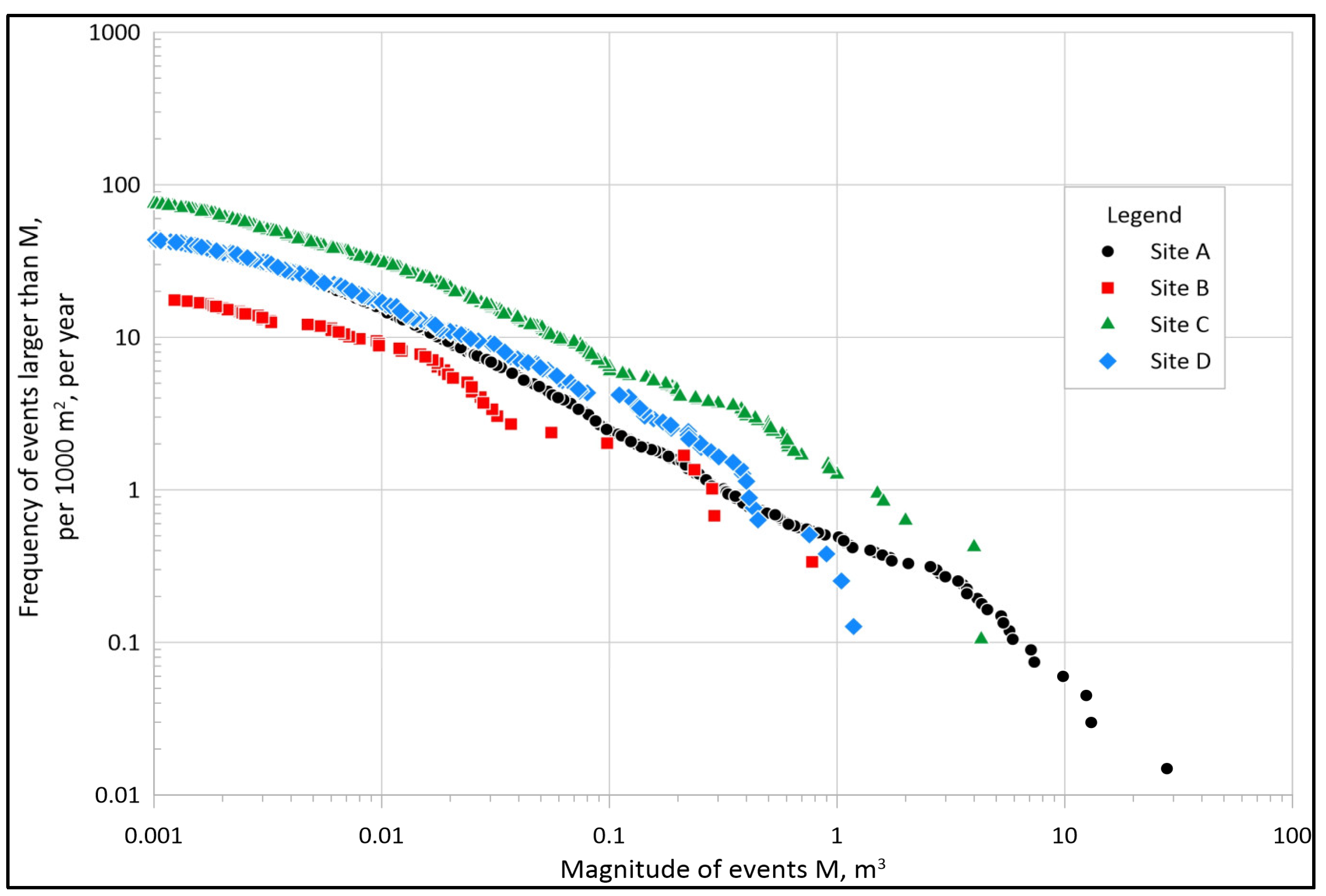
Figure 7.
Cumulative magnitude–frequency distributions for the four study sites over four or five years, per 1000 m2 of slope area, per year (2013 to 2017 for Site A; 2012 to 2017 for Sites B, C and D).
Figure 7.
Cumulative magnitude–frequency distributions for the four study sites over four or five years, per 1000 m2 of slope area, per year (2013 to 2017 for Site A; 2012 to 2017 for Sites B, C and D).
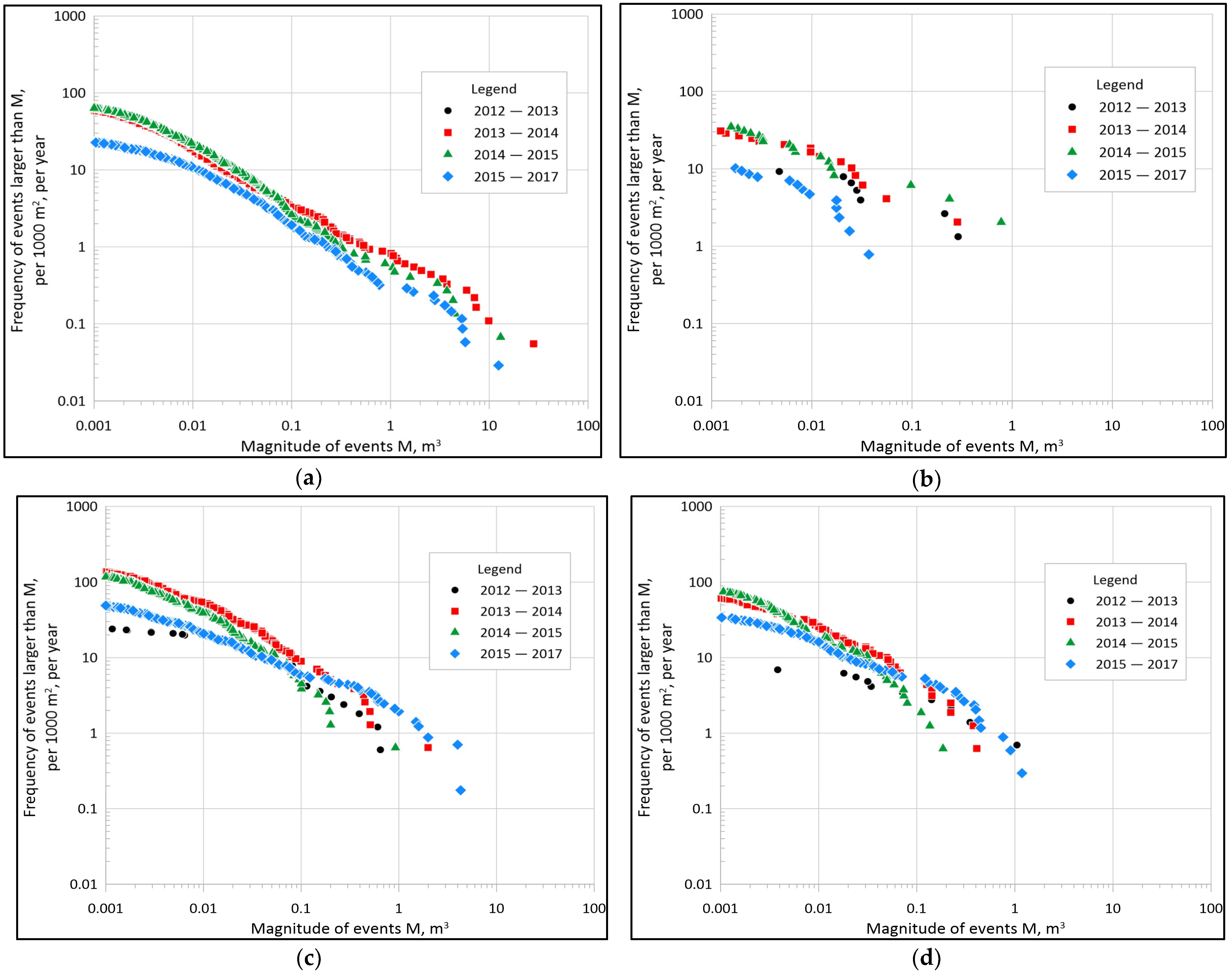
Figure 8.
Cumulative magnitude–frequency distributions at each site for each epoch: (a) Site A; (b) Site B; (c) Site C; (d) Site D.
Figure 8.
Cumulative magnitude–frequency distributions at each site for each epoch: (a) Site A; (b) Site B; (c) Site C; (d) Site D.
Figure 9.
Temporal variation in non-cumulative power–law parameters at each site: (a); Activity Parameter (β); (b) Scaling Parameter (α), per 1000 m2 of slope area (per year event frequency for the 2015–2017 epoch was divided by two).
Figure 9.
Temporal variation in non-cumulative power–law parameters at each site: (a); Activity Parameter (β); (b) Scaling Parameter (α), per 1000 m2 of slope area (per year event frequency for the 2015–2017 epoch was divided by two).
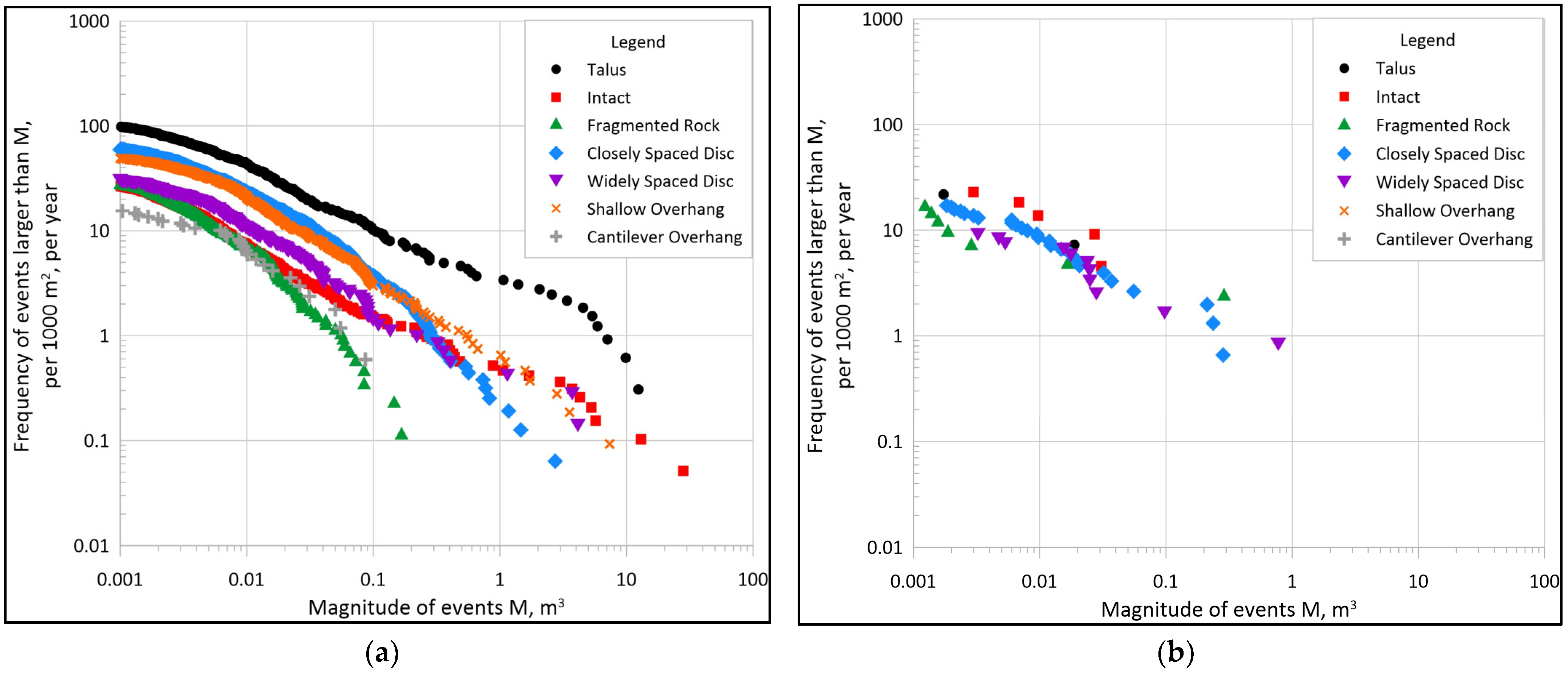
Figure 10.
Cumulative magnitude–frequency distributions at each site for each RAI class: (a) Site A; (b) Site B; (c) Site C; (d) Site D.
Figure 10.
Cumulative magnitude–frequency distributions at each site for each RAI class: (a) Site A; (b) Site B; (c) Site C; (d) Site D.
Figure 11.
Temporal variation of annual failure rate by RAI class (2012 to 2013 data omitted for all sites; 2014 to 2015 data omitted for Site D, described above): (a) Site A; (b) Site B; (c) Site C; (d) Site D.
Figure 11.
Temporal variation of annual failure rate by RAI class (2012 to 2013 data omitted for all sites; 2014 to 2015 data omitted for Site D, described above): (a) Site A; (b) Site B; (c) Site C; (d) Site D.
Figure 12.
Temporal variation of average failure depth by RAI class (2012 to 2013 data omitted for all sites; 2014 to 2015 data omitted for Site D, described above): (a) Site A; (b) Site B; (c) Site C; (d) Site D.
Figure 12.
Temporal variation of average failure depth by RAI class (2012 to 2013 data omitted for all sites; 2014 to 2015 data omitted for Site D, described above): (a) Site A; (b) Site B; (c) Site C; (d) Site D.
Figure 13.
Histogram of talus slope angle for Sites A, C, and D.
Figure 13.
Histogram of talus slope angle for Sites A, C, and D.
Table 1.
Original definitions of the 7 RAI classes and their preliminary estimated annual failure rates and average failure depths (after Dunham et al. [
13]).
Table 1.
Original definitions of the 7 RAI classes and their preliminary estimated annual failure rates and average failure depths (after Dunham et al. [
13]).
| RAI Class | Description | Preliminary Annual Failure Rate (r) | Preliminary Average
Failure Depth (D) (m) |
|---|
| Talus (T) | Mass wasting-derived rock fragments (debris) accumulated at the base of a slope or along benches within a slope | 0.0000 | 0.025 |
| Intact (I) | Rock mass with few or relatively minor discontinuities | 0.0010 | 0.05 |
| Fragmented Discontinuous Rock (Df) | Intact blocks or fragments of rock separated by discontinuities with a typical spacing of less than ~10 cm | 0.0018 | 0.1 |
| Closely Spaced Discontinuous Rock (Dc) | Intact blocks or fragments of rock separated by discontinuities typically spaced between ~10 cm and ~20 cm | 0.0034 | 0.2 |
| Widely Spaced Discontinuous Rock (Dw) | Intact blocks or fragments of rock separated by discontinuities typically spaced at ~30 cm or greater | 0.0071 | 0.3 |
| Shallow Overhang (Os) | Overhanging rock whose lower portion is inclined at less than 120 degrees | 0.0197 | 0.75 |
| Cantilever Overhang (Oc) | Overhanging rock whose lower portion is inclined at greater (i.e., steeper) than 120 degrees | 0.0198 | 0.5 |
Table 2.
Non-cumulative Activity Parameters (β) and Scaling Parameters (α) for each site across four or five years, per 1000 m2 of slope area, per year (2013 to 2017 for Site A; 2012 to 2017 for Sites B, C, and D).
Table 2.
Non-cumulative Activity Parameters (β) and Scaling Parameters (α) for each site across four or five years, per 1000 m2 of slope area, per year (2013 to 2017 for Site A; 2012 to 2017 for Sites B, C, and D).
| Site | Activity Parameter, β | Scaling Parameter, α |
|---|
| Site A | 0.344 | 1.770 |
| Site B | 0.305 | 1.566 |
| Site C | 0.945 | 1.686 |
| Site D | 0.444 | 1.756 |
Table 3.
Non-cumulative Activity Parameters (β) and Scaling Parameters (α) for each epoch, for each site, per 1000 m2 of slope area (per year event frequency for the 2015–2017 epoch was halved). 1 N/A indicates data not available; an initial 2012 scan was not completed at Site A.
Table 3.
Non-cumulative Activity Parameters (β) and Scaling Parameters (α) for each epoch, for each site, per 1000 m2 of slope area (per year event frequency for the 2015–2017 epoch was halved). 1 N/A indicates data not available; an initial 2012 scan was not completed at Site A.
| Epoch | Site A | Site B | Site C | Site D |
|---|
| β | α | β | α | β | α | β | α |
|---|
| 2012–2013 | N/A 1 | N/A 1 | 0.454 | 1.524 | 0.646 | 1.754 | 0.443 | 1.513 |
| 2013–2014 | 0.478 | 1.717 | 0.668 | 1.494 | 1.157 | 1.787 | 0.547 | 1.814 |
| 2014–2015 | 0.416 | 1.805 | 0.849 | 1.445 | 0.557 | 1.914 | 0.268 | 1.936 |
| 2015–2017 | 0.261 | 1.759 | 0.108 | 1.610 | 0.963 | 1.543 | 0.616 | 1.598 |
Table 4.
Non-cumulative Activity Parameters (β) and Scaling Parameters (α) for each RAI class at each site, averaged across the years of evaluation, per 1000 m2 of slope area. 1 N/A indicates too few rockfall events occurred within this RAI class to deduce power–law parameters.
Table 4.
Non-cumulative Activity Parameters (β) and Scaling Parameters (α) for each RAI class at each site, averaged across the years of evaluation, per 1000 m2 of slope area. 1 N/A indicates too few rockfall events occurred within this RAI class to deduce power–law parameters.
| RAI Class | Site A | Site B | Site C | Site D |
|---|
| β | α | β | α | β | α | β | α |
|---|
| Talus (T) | 1.729 | 1.535 | 0.565 | 1.419 | 1.513 | 1.291 | 1.517 | 1.449 |
| Intact (I) | 0.256 | 1.632 | 0.477 | 1.601 | 0.538 | 1.764 | 0.219 | 1.797 |
| Fragmented Discontinuous Rock (Df) | 0.064 | 1.966 | 0.453 | 1.346 | 0.608 | 1.655 | 0.126 | 1.754 |
| Closely Spaced Discontinuous Rock (Dc) | 0.432 | 1.833 | 0.321 | 1.564 | 1.278 | 1.648 | 0.595 | 1.691 |
| Widely Spaced Discontinuous Rock (Dw) | 0.264 | 1.734 | 0.320 | 1.468 | 0.395 | 1.620 | 0.769 | 1.655 |
| Shallow Overhang (Os) | 0.457 | 1.773 | N/A 1 | N/A 1 | 0.853 | 1.401 | 0.342 | 1.774 |
| Cantilever Overhang (Oc) | 0.202 | 1.589 | N/A 1 | N/A 1 | N/A 1 | N/A 1 | N/A 1 | N/A 1 |
Table 5.
Average, Standard Deviation, and Coefficient of Variation (CoV) of non-cumulative Activity Parameter (β) and Scaling Parameter (α) for each RAI class.
Table 5.
Average, Standard Deviation, and Coefficient of Variation (CoV) of non-cumulative Activity Parameter (β) and Scaling Parameter (α) for each RAI class.
| RAI Class | Average β | St. Dev. β | CoV β | Average α | St. Dev. α | CoV α |
|---|
| Talus (T) | 1.331 | 0.451 | 0.339 | 1.424 | 0.088 | 0.062 |
| Intact (I) | 0.373 | 0.137 | 0.369 | 1.699 | 0.084 | 0.049 |
| Fragmented Discontinuous Rock (Df) | 0.313 | 0.226 | 0.721 | 1.585 | 0.174 | 0.110 |
| Closely Spaced Discontinuous Rock (Dc) | 0.657 | 0.372 | 0.566 | 1.684 | 0.097 | 0.058 |
| Widely Spaced Discontinuous Rock (Dw) | 0.437 | 0.197 | 0.451 | 1.619 | 0.097 | 0.060 |
| Shallow Overhang (Os) | 0.551 | 0.219 | 0.397 | 1.649 | 0.176 | 0.106 |
| Cantilever Overhang (Oc) | 0.202 | N/A | N/A | 1.589 | N/A | N/A |
Table 6.
Annual failure rate (r) and average failure depth (D) for each RAI class, averaged across all epochs; 2012 to 2013 data omitted for all sites, and 2014 to 2015 data omitted for Site D.
Table 6.
Annual failure rate (r) and average failure depth (D) for each RAI class, averaged across all epochs; 2012 to 2013 data omitted for all sites, and 2014 to 2015 data omitted for Site D.
| RAI Class | Site A | Site B | Site C | Site D |
|---|
| r | D | r | D | r | D | r | D |
|---|
| Talus (T) | 0.140 | −0.169 | 0.021 | −0.063 | 0.176 | −0.090 | 0.089 | −0.082 |
| Intact (I) | 0.021 | −0.188 | 0.021 | −0.070 | 0.052 | −0.075 | 0.026 | −0.080 |
| Fragmented Discontinuous Rock (Df) | 0.025 | −0.189 | 0.032 | −0.103 | 0.077 | −0.087 | 0.042 | −0.116 |
| Closely Spaced Discontinuous Rock (Dc) | 0.031 | −0.190 | 0.031 | −0.098 | 0.075 | −0.095 | 0.034 | −0.119 |
| Widely Spaced Discontinuous Rock (Dw) | 0.033 | −0.249 | 0.019 | −0.130 | 0.043 | −0.122 | 0.020 | −0.140 |
| Shallow Overhang (Os) | 0.022 | −0.219 | 0.004 | −0.129 | 0.079 | −0.105 | 0.021 | −0.143 |
| Cantilever Overhang (Oc) | 0.038 | −0.236 | 0.007 | −0.198 | 0.081 | −0.207 | 0.026 | −0.175 |
Table 7.
Average, Standard Deviation, and Coefficient of Variation (CoV) of annual failure rate (r) and average failure depth (D, in meters) for each RAI class.
Table 7.
Average, Standard Deviation, and Coefficient of Variation (CoV) of annual failure rate (r) and average failure depth (D, in meters) for each RAI class.
| RAI Class | Average r | St. Dev. r | CoV r | Average D | St. Dev. D | CoV D |
|---|
| Talus (T) | 0.108 | 0.110 | 1.026 | −0.102 | 0.055 | −0.542 |
| Intact (I) | 0.030 | 0.017 | 0.563 | −0.105 | 0.059 | −0.569 |
| Fragmented Discontinuous Rock (Df) | 0.044 | 0.036 | 0.821 | −0.124 | 0.053 | −0.429 |
| Closely Spaced Discontinuous Rock (Dc) | 0.043 | 0.032 | 0.743 | −0.126 | 0.055 | −0.434 |
| Widely Spaced Discontinuous Rock (Dw) | 0.029 | 0.022 | 0.766 | −0.162 | 0.080 | −0.492 |
| Shallow Overhang (Os) | 0.032 | 0.045 | 1.403 | −0.149 | 0.058 | −0.390 |
| Cantilever Overhang (Oc) | 0.041 | 0.066 | 1.610 | −0.206 | 0.059 | −0.284 |
Table 8.
Average of annual failure rates and average failure depths, averaged across all sites and epochs; 2012 to 2013 data omitted for all sites, and 2014 to 2015 data omitted for Site D; weighted by site area.
Table 8.
Average of annual failure rates and average failure depths, averaged across all sites and epochs; 2012 to 2013 data omitted for all sites, and 2014 to 2015 data omitted for Site D; weighted by site area.
| RAI Class | Average Annual Failure Rate, r | Average Failure Depth, D (m) |
|---|
| Talus (T) | 0.137 | −0.153 |
| Intact (I) | 0.024 | −0.167 |
| Fragmented Discontinuous Rock (Df) | 0.031 | −0.173 |
| Closely Spaced Discontinuous Rock (Dc) | 0.035 | −0.175 |
| Widely Spaced Discontinuous Rock (Dw) | 0.032 | −0.227 |
| Shallow Overhang (Os) | 0.027 | −0.202 |
| Cantilever Overhang (Oc) | 0.040 | −0.229 |
Table 9.
Recommended Annual Failure Rates and Average Failure Depths for use in the RAI framework.
Table 9.
Recommended Annual Failure Rates and Average Failure Depths for use in the RAI framework.
| RAI Class | Annual Failure Rate, r | Average Failure Depth, D (m) |
|---|
| Talus (T) | 0.137 | −0.153 |
| Intact (I) | 0.024 | −0.167 |
| Fragmented Discontinuous Rock (Df) | 0.031 | −0.173 |
| Closely Spaced Discontinuous Rock (Dc) | 0.035 | −0.175 |
| Widely Spaced Discontinuous Rock (Dw) | 0.032 | −0.227 |
| Shallow Overhang (Os) | 0.027 | −0.202 |
| Cantilever Overhang (Oc) | 0.040 | −0.229 |


