
Filtering Green Vegetation Out from Colored Point Clouds of Rocky Terrains Based on Various Vegetation Indices: Comparison of Simple Statistical Methods, Support Vector Machine, and Neural Network

Abstract
:1. Introduction
2. Materials and Methods
2.1. The Test Data
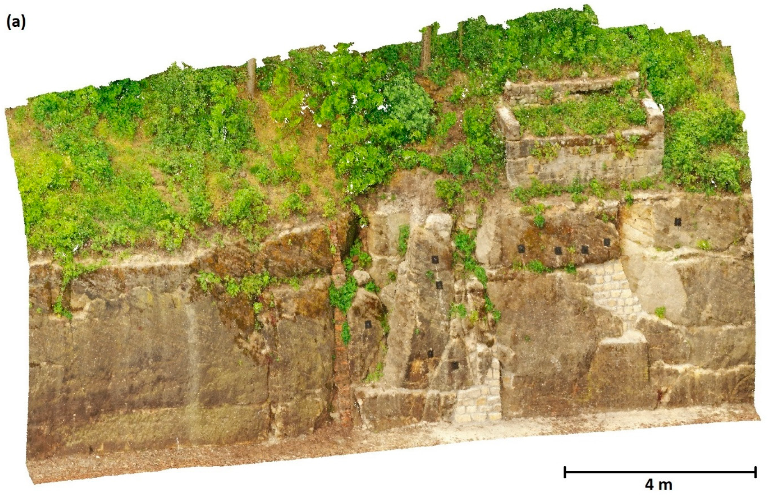
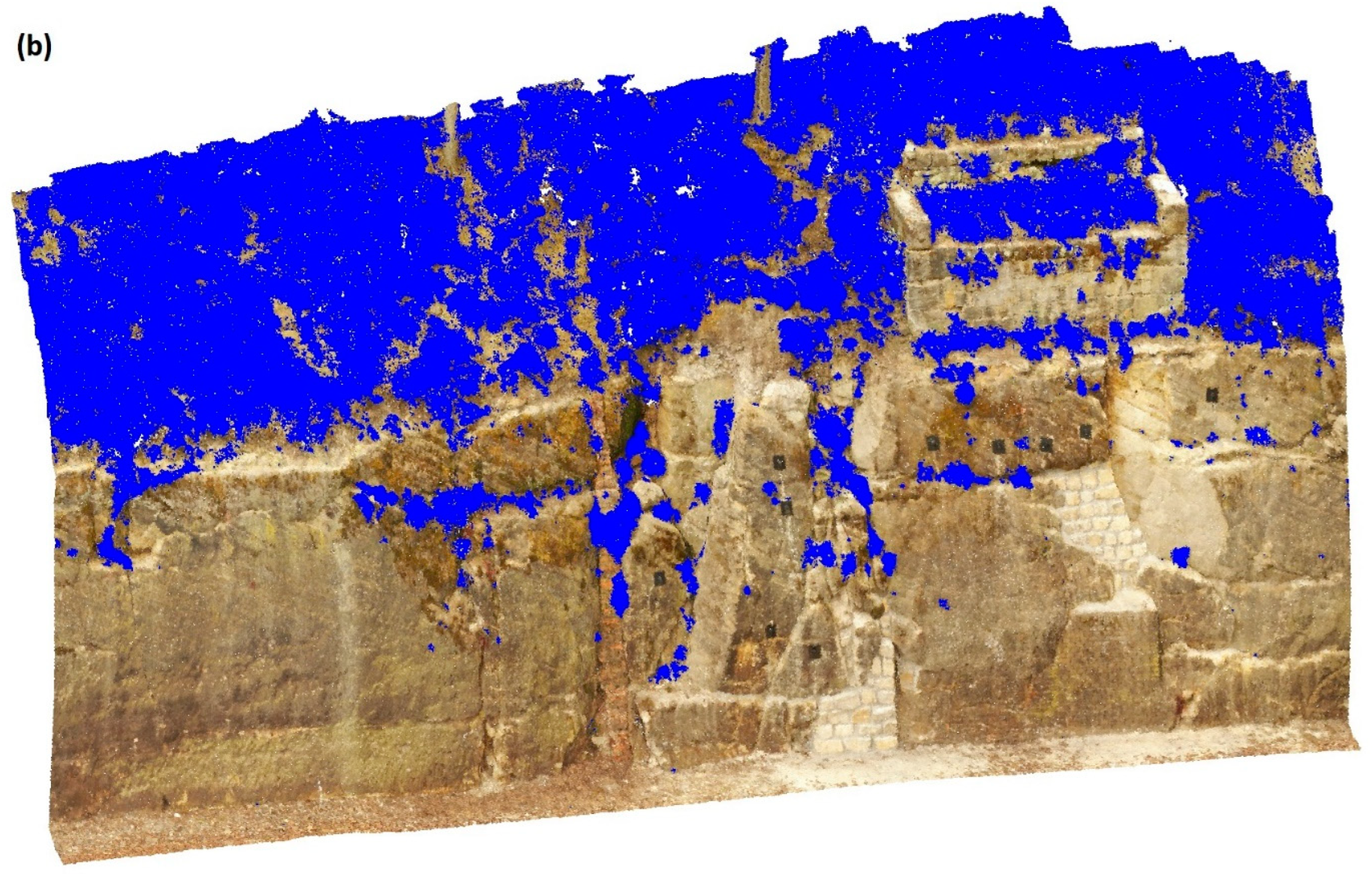
2.1.1. Data 1
2.1.2. Data 2
2.1.3. Data 3
2.1.4. Data 4
2.2. Vegetation Indices Tested
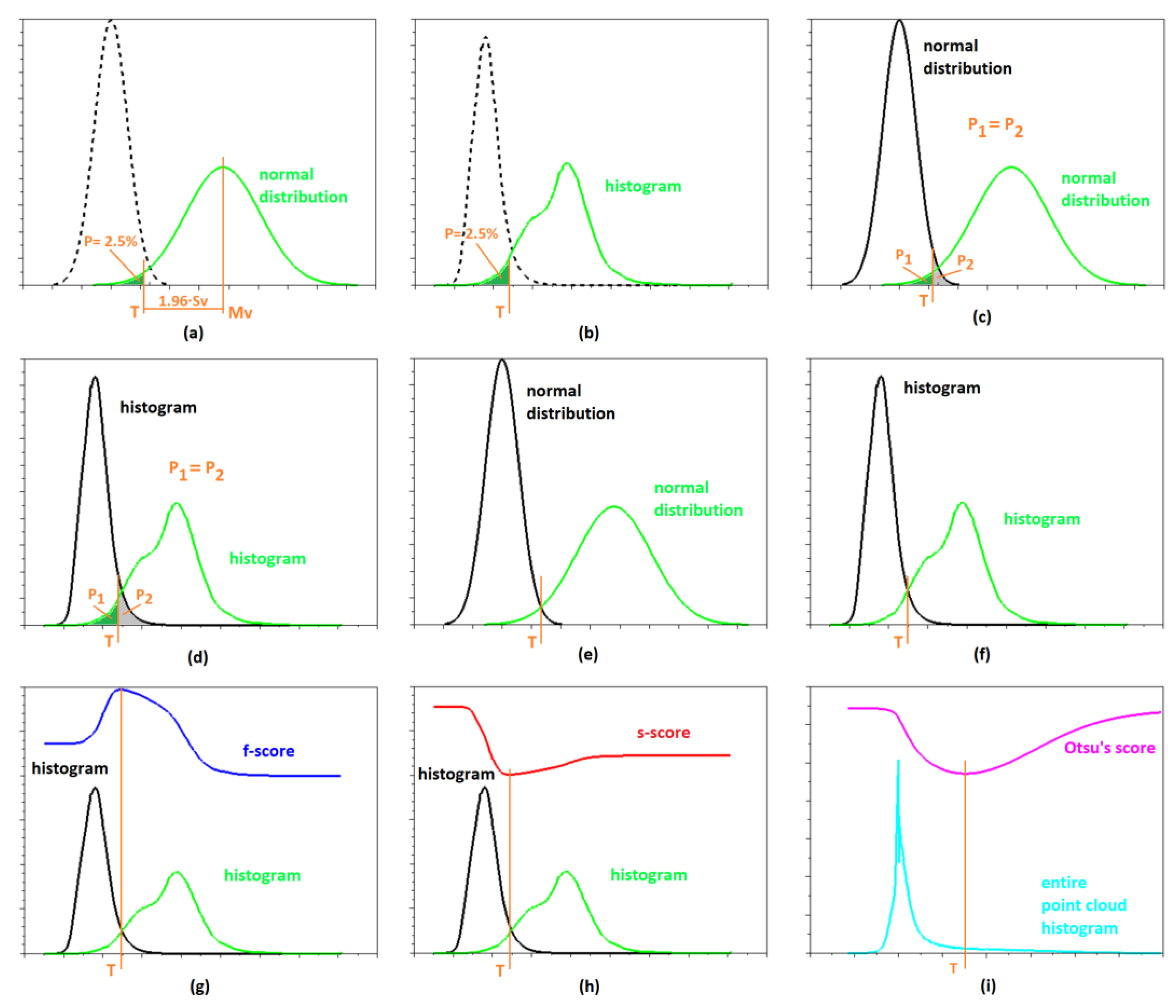
2.3. Methods of the Threshold Determination
2.3.1. Data Distribution and Training Datasets
2.3.2. Single Class Method Based on Normal Distribution Assumption (SCND)
- The mean (M) and standard deviation (SD) are determined from the VI values of the training set.
- The threshold T is calculated using the formula T = M + 1.96·SD or T = M − 1.96·SD; whether plus or minus is used depends on the orientation of the particular VI (if vegetation has higher values of VI than other points, the minus sign is applied, and vice versa).
- All points that exceed this threshold are removed from the cloud.
2.3.3. Single Class Method Based on Histogram Calculation (SCHC)
2.3.4. Two-Class Method Based on the Normal Distribution Assumption (TCND)
2.3.5. Two-Class Method Based on Histogram Calculation (TCHC)
2.3.6. Two-Class Methods Based on the Score Function Evaluation (TCSF)
2.3.7. Two-Class Method Based on the Support Vector Machine (SVM)
2.3.8. Two-Class Method Based on a Neural Network (DNN)
2.3.9. Two-Class Multi-VI Method Based on the Support Vector Machine (MSVM)
2.3.10. Two-Class Multi-VI Method Based on Neural Network (MDNN)
2.3.11. Otsu’s Method (Otsu)
2.4. Testing of the Methods
3. Results
4. Discussion
5. Conclusions
Author Contributions
Funding
Institutional Review Board Statement
Informed Consent Statement
Data Availability Statement
Conflicts of Interest
Appendix A. Reference Data Created by a Human Operator


Appendix B. Histograms for Individual Vegetation Indices—Data 1

Appendix C. Detailed Evaluation Results

| VVI | SCND | SCHC | TCND p | TCND i | TCHCp | TCHC i | TCSF f | TCSF s | SVM | DNN | Otsu | Mean |
|---|---|---|---|---|---|---|---|---|---|---|---|---|
| ExG | 98.8 | 86.3 | 92.0 | 96.9 | 94.6 | 99.3 | 94.0 | 96.3 | 89.0 | 94.0 | 79.8 | 92.8 |
| ExR | 63.9 | 80.2 | 83.4 | 81.4 | 82.5 | 84.3 | 83.3 | 84.2 | 78.7 | 83.3 | 72.8 | 79.8 |
| ExB | 80.6 | 86.4 | 86.4 | 87.7 | 88.6 | 87.8 | 86.5 | 86.5 | 83.5 | 86.0 | 87.4 | 86.1 |
| ExGr | 95.0 | 88.5 | 93.7 | 92.0 | 94.0 | 94.6 | 91.8 | 92.4 | 88.8 | 91.5 | 76.7 | 90.8 |
| GRVI | 85.1 | 87.1 | 86.9 | 84.0 | 86.4 | 87.1 | 85.2 | 86.8 | 81.7 | 85.3 | 75.3 | 84.6 |
| MGRVI | 86.8 | 87.1 | 87.2 | 84.2 | 86.3 | 87.1 | 85.2 | 86.8 | 83.3 | 85.3 | 77.0 | 85.1 |
| RGBVI | 87.1 | 86.1 | 95.8 | 96.6 | 94.0 | 97.2 | 95.4 | 95.4 | 90.7 | 93.9 | 85.1 | 92.5 |
| IKAW | 32.4 | 32.4 | 33.3 | 33.6 | 33.1 | 33.4 | 33.5 | 33.0 | 32.6 | 32.6 | 33.6 | 33.1 |
| VARI | 83.8 | 84.2 | 84.7 | 82.6 | 84.2 | 84.8 | 82.9 | 84.2 | 81.6 | 83.4 | 75.6 | 82.9 |
| CIVE | 86.4 | 84.6 | 93.3 | 91.0 | 93.1 | 92.8 | 92.5 | 92.5 | 92.3 | 91.2 | 82.6 | 90.2 |
| GLI | 93.3 | 86.1 | 93.7 | 96.5 | 94.4 | 98.9 | 94.0 | 96.3 | 87.7 | 94.0 | 81.6 | 92.4 |
| VEG | 38.5 | 87.8 | 88.8 | 93.9 | 95.7 | 94.8 | 92.9 | 92.9 | 89.4 | 93.0 | 71.2 | 85.4 |
| VVI | SCND | SCHC | TCND p | TCND i | TCHCp | TCHC i | TCSF f | TCSF s | SVM | DNN | Otsu | Mean |
|---|---|---|---|---|---|---|---|---|---|---|---|---|
| ExG | 99.3 | 97.0 | 92.6 | 98.9 | 94.9 | 99.5 | 98.3 | 98.8 | 97.4 | 98.3 | 96.0 | 97.4 |
| ExR | 73.2 | 85.6 | 89.6 | 94.8 | 88.3 | 93.1 | 94.2 | 93.4 | 95.0 | 94.2 | 94.7 | 90.6 |
| ExB | 84.0 | 94.5 | 89.1 | 94.0 | 92.4 | 93.9 | 94.5 | 94.5 | 94.9 | 94.6 | 94.1 | 92.8 |
| ExGr | 97.0 | 97.1 | 94.7 | 97.6 | 95.1 | 97.4 | 97.5 | 97.6 | 97.2 | 97.5 | 95.5 | 96.8 |
| GRVI | 89.3 | 92.6 | 92.0 | 95.3 | 91.0 | 93.7 | 95.1 | 94.3 | 95.4 | 95.0 | 95.0 | 93.5 |
| MGRVI | 94.3 | 92.8 | 93.1 | 95.2 | 90.8 | 93.7 | 95.1 | 94.3 | 95.3 | 95.0 | 95.2 | 94.1 |
| RGBVI | 97.1 | 97.0 | 95.9 | 98.8 | 94.4 | 98.9 | 98.6 | 98.6 | 97.7 | 98.3 | 96.8 | 97.5 |
| IKAW | 21.9 | 23.3 | 53.6 | 53.7 | 53.5 | 53.6 | 53.7 | 53.5 | 9.7 | 9.7 | 53.7 | 40.0 |
| VARI | 88.9 | 89.5 | 90.7 | 94.1 | 89.6 | 92.5 | 94.0 | 93.3 | 94.3 | 93.8 | 94.5 | 92.3 |
| CIVE | 96.6 | 96.4 | 95.6 | 97.0 | 95.0 | 96.7 | 96.8 | 96.8 | 96.9 | 97.0 | 96.1 | 96.4 |
| GLI | 98.2 | 96.9 | 94.1 | 98.9 | 94.7 | 99.4 | 98.3 | 98.8 | 97.2 | 98.3 | 96.3 | 97.4 |
| VEG | 61.9 | 97.1 | 89.9 | 98.1 | 96.1 | 98.1 | 97.9 | 97.9 | 97.4 | 97.9 | 94.9 | 93.4 |
| MSVM | MDNN | Mean | ||||
|---|---|---|---|---|---|---|
| FS [%] | BA [%] | FS [%] | BA [%] | FS [%] | BA [%] | |
| ExG, ExGr, RBVI, CIVE, GLI | 91.7 | 97.0 | 91.7 | 97.1 | 91.7 | 97.0 |
| ExG, ExGr, RBVI, CIVE, VEG | 91.7 | 97.0 | 92.3 | 97.1 | 92.0 | 97.0 |
| ExG, RBVI, GLI | 89.6 | 97.5 | 92.7 | 97.6 | 91.1 | 97.5 |
| ExG, RBVI, CIVE | 91.9 | 96.9 | 90.4 | 96.7 | 91.2 | 96.8 |
| ExG, GLI, VEG | 89.0 | 97.4 | 93.5 | 98.3 | 91.3 | 97.9 |
| ExG, GLI | 88.5 | 97.3 | 93.9 | 98.3 | 91.2 | 97.8 |
| VVI | SCND | SCHC | TCND p | TCND i | TCHCp | TCHC i | TCSF f | TCSF s | SVM | DNN | Otsu | Mean |
|---|---|---|---|---|---|---|---|---|---|---|---|---|
| ExG | 99.7 | 95.4 | 90.0 | 90.3 | 94.8 | 96.0 | 95.4 | 94.8 | 97.3 | 95.1 | 90.0 | 94.4 |
| ExR | 81.3 | 88.3 | 81.7 | 83.7 | 88.5 | 87.5 | 88.1 | 88.5 | 88.5 | 88.2 | 85.2 | 86.3 |
| ExB | 87.7 | 90.1 | 92.0 | 92.5 | 88.6 | 90.0 | 88.9 | 87.5 | 88.9 | 88.6 | 91.0 | 89.6 |
| ExGr | 97.3 | 92.2 | 87.8 | 88.3 | 95.6 | 97.5 | 95.9 | 95.9 | 97.8 | 96.1 | 88.8 | 93.9 |
| GRVI | 93.1 | 90.7 | 85.5 | 86.7 | 93.0 | 92.4 | 93.0 | 93.2 | 92.4 | 92.8 | 88.0 | 91.0 |
| MGRVI | 93.1 | 90.7 | 85.9 | 87.0 | 93.0 | 92.4 | 93.0 | 93.2 | 92.6 | 92.8 | 88.7 | 91.1 |
| RGBVI | 97.0 | 97.1 | 94.7 | 95.0 | 93.1 | 94.2 | 93.2 | 93.0 | 93.9 | 93.3 | 94.9 | 94.5 |
| IKAW | 57.7 | 60.3 | 79.3 | 79.6 | 75.1 | 78.2 | 75.9 | 74.8 | 77.7 | 77.0 | 75.4 | 73.7 |
| VARI | 93.5 | 90.7 | 87.6 | 88.8 | 93.6 | 92.8 | 93.7 | 93.7 | 93.3 | 93.5 | 91.2 | 92.0 |
| CIVE | 93.5 | 93.5 | 90.8 | 91.0 | 95.1 | 95.7 | 95.2 | 95.2 | 95.3 | 95.2 | 91.3 | 93.8 |
| GLI | 98.1 | 95.4 | 91.5 | 91.8 | 94.9 | 96.0 | 95.4 | 94.8 | 97.4 | 95.1 | 91.8 | 94.7 |
| VEG | 55.3 | 97.1 | 80.8 | 83.3 | 94.2 | 96.2 | 94.5 | 93.7 | 96.6 | 94.4 | 74.3 | 87.3 |
| VVI | SCND | SCHC | TCND p | TCND i | TCHCp | TCHC i | TCSF f | TCSF s | SVM | DNN | Otsu | Mean |
|---|---|---|---|---|---|---|---|---|---|---|---|---|
| ExG | 99.7 | 97.4 | 94.8 | 95.0 | 95.1 | 96.2 | 95.6 | 95.1 | 97.3 | 95.4 | 94.9 | 96.0 |
| ExR | 83.5 | 91.7 | 91.8 | 92.4 | 93.1 | 93.4 | 93.4 | 93.1 | 93.0 | 93.3 | 92.9 | 92.0 |
| ExB | 89.1 | 91.0 | 94.8 | 94.9 | 89.8 | 90.9 | 90.0 | 88.9 | 90.0 | 89.7 | 94.5 | 91.2 |
| ExGr | 98.2 | 95.8 | 94.0 | 94.2 | 95.8 | 97.7 | 96.1 | 96.1 | 98.1 | 96.3 | 94.4 | 96.1 |
| GRVI | 94.9 | 95.1 | 93.1 | 93.6 | 95.7 | 95.6 | 95.7 | 95.7 | 95.6 | 95.7 | 94.0 | 95.0 |
| MGRVI | 95.6 | 95.1 | 93.2 | 93.7 | 95.6 | 95.6 | 95.7 | 95.7 | 95.7 | 95.7 | 94.3 | 95.1 |
| RGBVI | 97.6 | 97.6 | 96.8 | 96.9 | 93.5 | 94.5 | 93.6 | 93.5 | 94.2 | 93.8 | 96.8 | 95.3 |
| IKAW | 69.9 | 70.8 | 83.0 | 82.4 | 78.5 | 80.7 | 79.0 | 78.3 | 80.3 | 79.8 | 83.4 | 78.7 |
| VARI | 95.9 | 95.0 | 93.8 | 94.3 | 96.0 | 95.8 | 96.0 | 96.0 | 95.9 | 95.9 | 95.2 | 95.4 |
| CIVE | 96.3 | 96.3 | 95.2 | 95.3 | 95.6 | 96.3 | 95.6 | 95.6 | 95.8 | 95.7 | 95.4 | 95.7 |
| GLI | 98.8 | 97.4 | 95.5 | 95.6 | 95.1 | 96.1 | 95.6 | 95.1 | 97.5 | 95.4 | 95.6 | 96.1 |
| VEG | 19.4 | 98.2 | 91.6 | 92.4 | 94.5 | 96.4 | 94.8 | 94.1 | 96.8 | 94.8 | 89.8 | 87.5 |
| MSVM | MDNN | Mean | ||||
|---|---|---|---|---|---|---|
| FS [%] | BA [%] | FS [%] | BA [%] | FS [%] | BA [%] | |
| ExG, ExGr, RBVI, CIVE, GLI | 95.9 | 96.3 | 95.0 | 95.2 | 95.4 | 95.8 |
| ExG, ExGr, RBVI, CIVE, VEG | 96.1 | 96.4 | 94.1 | 94.5 | 95.1 | 95.5 |
| ExG, RBVI, GLI | 95.9 | 96.1 | 95.3 | 95.5 | 95.6 | 95.8 |
| ExG, RBVI, CIVE | 95.8 | 96.2 | 96.0 | 96.2 | 95.9 | 96.2 |
| ExG, GLI, VEG | 97.1 | 97.2 | 94.6 | 94.9 | 95.9 | 96.1 |
| ExG, GLI | 97.3 | 97.4 | 95.1 | 95.3 | 96.2 | 96.4 |
| VVI | SCND | SCHC | TCND p | TCND i | TCHCp | TCHC i | TCSF f | TCSF s | SVM | DNN | Otsu | Mean |
|---|---|---|---|---|---|---|---|---|---|---|---|---|
| ExG | 98.1 | 91.5 | 82.2 | 86.6 | 95.1 | 93.4 | 96.9 | 97.3 | 95.2 | 96.1 | 96.5 | 93.5 |
| ExR | 53.7 | 50.9 | 52.0 | 53.7 | 52.9 | 53.8 | 50.8 | 49.9 | 51.2 | 49.6 | 28.9 | 49.8 |
| ExB | 38.3 | 51.4 | 58.0 | 63.4 | 59.4 | 57.4 | 59.9 | 63.1 | 63.8 | 61.3 | 64.8 | 58.3 |
| ExGr | 82.0 | 79.9 | 86.3 | 86.0 | 85.6 | 85.9 | 84.6 | 83.8 | 84.5 | 84.5 | 80.7 | 84.0 |
| GRVI | 62.6 | 63.9 | 61.7 | 63.2 | 63.2 | 63.8 | 60.2 | 60.2 | 60.4 | 59.6 | 38.6 | 59.8 |
| MGRVI | 62.6 | 63.9 | 61.9 | 63.2 | 63.2 | 63.8 | 60.2 | 60.2 | 60.7 | 59.9 | 43.7 | 60.3 |
| RGBVI | 83.7 | 88.2 | 75.6 | 80.2 | 85.9 | 84.2 | 85.0 | 86.2 | 84.9 | 85.1 | 86.7 | 84.2 |
| IKAW | 21.6 | 22.9 | 30.3 | 28.9 | 29.5 | 31.0 | 27.7 | 32.5 | 7.5 | 34.2 | 33.5 | 27.2 |
| VARI | 64.8 | 68.3 | 65.6 | 67.1 | 66.8 | 68.8 | 64.0 | 64.0 | 64.6 | 64.8 | 63.4 | 65.7 |
| CIVE | 86.0 | 85.0 | 88.9 | 89.8 | 85.8 | 86.5 | 88.1 | 88.1 | 88.5 | 88.1 | 88.3 | 87.6 |
| GLI | 97.1 | 91.4 | 83.1 | 87.0 | 95.2 | 93.4 | 96.9 | 97.3 | 95.2 | 96.0 | 91.4 | 93.1 |
| VEG | 94.5 | 89.9 | 82.7 | 89.3 | 96.4 | 96.1 | 96.0 | 96.0 | 96.6 | 96.5 | 96.3 | 93.7 |
| VVI | SCND | SCHC | TCND p | TCND i | TCHCp | TCHC i | TCSF f | TCSF s | SVM | DNN | Otsu | Mean |
|---|---|---|---|---|---|---|---|---|---|---|---|---|
| ExG | 99.0 | 98.4 | 84.9 | 88.2 | 95.6 | 94.0 | 97.4 | 97.8 | 95.7 | 96.6 | 97.0 | 95.0 |
| ExR | 72.0 | 67.7 | 74.7 | 72.2 | 73.7 | 72.1 | 75.8 | 76.5 | 75.5 | 76.6 | 57.5 | 72.2 |
| ExB | 61.8 | 67.2 | 70.5 | 73.6 | 71.3 | 70.2 | 71.5 | 73.4 | 73.8 | 72.3 | 74.5 | 70.9 |
| ExGr | 95.9 | 96.2 | 94.0 | 94.5 | 94.7 | 94.5 | 95.3 | 95.5 | 95.3 | 95.3 | 84.7 | 94.2 |
| GRVI | 81.1 | 77.6 | 82.0 | 80.2 | 80.2 | 78.7 | 83.6 | 83.6 | 83.1 | 84.0 | 61.6 | 79.6 |
| MGRVI | 81.1 | 77.5 | 81.9 | 80.2 | 80.2 | 78.7 | 83.6 | 83.6 | 82.9 | 83.8 | 63.6 | 79.7 |
| RGBVI | 86.2 | 90.9 | 80.4 | 83.5 | 88.1 | 86.6 | 87.3 | 88.4 | 87.2 | 87.4 | 88.9 | 86.8 |
| IKAW | 55.3 | 55.6 | 57.2 | 56.9 | 57.0 | 57.3 | 56.6 | 57.8 | 57.8 | 59.0 | 58.3 | 57.2 |
| VARI | 84.5 | 81.8 | 84.0 | 82.9 | 83.0 | 81.1 | 85.0 | 85.0 | 84.5 | 84.4 | 73.8 | 82.7 |
| CIVE | 98.5 | 98.4 | 91.0 | 92.1 | 87.9 | 88.5 | 90.1 | 90.1 | 90.5 | 90.1 | 90.3 | 91.6 |
| GLI | 98.9 | 98.4 | 85.5 | 88.5 | 95.7 | 94.0 | 97.4 | 97.8 | 95.7 | 96.5 | 92.2 | 94.6 |
| VEG | 95.0 | 97.8 | 85.3 | 90.3 | 97.6 | 96.7 | 97.7 | 97.7 | 97.3 | 97.5 | 96.9 | 95.4 |
| MSVM | MDNN | Mean | ||||
|---|---|---|---|---|---|---|
| FS [%] | BA [%] | FS [%] | BA [%] | FS [%] | BA [%] | |
| ExG, ExGr, RBVI, CIVE, GLI | 89.6 | 91.4 | 91.4 | 95.6 | 90.5 | 93.5 |
| ExG, ExGr, RBVI, CIVE, VEG | 90.0 | 91.7 | 90.5 | 95.2 | 90.3 | 93.5 |
| ExG, RBVI, GLI | 92.7 | 93.4 | 94.0 | 97.2 | 93.4 | 95.3 |
| ExG, RBVI, CIVE | 89.1 | 90.9 | 94.0 | 95.7 | 91.6 | 93.3 |
| ExG, GLI, VEG | 96.0 | 96.6 | 96.5 | 97.1 | 96.3 | 96.8 |
| ExG, GLI | 95.2 | 95.7 | 96.4 | 96.9 | 95.8 | 96.3 |
| VVI | SCND | SCHC | TCND p | TCND i | TCHCp | TCHC i | TCSF f | TCSF s | SVM | DNN | Otsu | Mean |
|---|---|---|---|---|---|---|---|---|---|---|---|---|
| ExG | 94.2 | 97.4 | 99.2 | 92.9 | 89.5 | 91.7 | 91.4 | 90.4 | 94.4 | 91.2 | 75.6 | 91.6 |
| ExR | 77.3 | 78.7 | 72.9 | 69.8 | 70.6 | 78.2 | 78.7 | 78.1 | 74.5 | 78.6 | 71.5 | 75.4 |
| ExB | 67.8 | 63.0 | 80.2 | 81.1 | 71.6 | 76.6 | 76.3 | 74.0 | 79.0 | 76.8 | 82.1 | 75.3 |
| ExGr | 89.8 | 90.2 | 88.0 | 84.0 | 88.0 | 83.6 | 86.0 | 86.6 | 87.1 | 85.4 | 73.8 | 85.7 |
| GRVI | 81.5 | 82.0 | 75.2 | 71.9 | 72.4 | 81.1 | 81.9 | 78.6 | 77.0 | 81.8 | 73.7 | 77.9 |
| MGRVI | 82.0 | 82.0 | 75.1 | 72.7 | 72.4 | 80.0 | 81.9 | 78.6 | 77.9 | 81.8 | 74.5 | 78.1 |
| RGBVI | 92.6 | 97.4 | 98.2 | 95.2 | 91.3 | 94.1 | 90.7 | 90.7 | 94.4 | 92.5 | 80.3 | 92.5 |
| IKAW | 45.3 | 45.4 | 42.5 | 42.6 | 43.1 | 42.8 | 43.0 | 42.6 | 43.1 | 36.1 | 42.1 | 42.6 |
| VARI | 47.5 | 80.1 | 72.8 | 62.9 | 68.1 | 76.1 | 80.3 | 79.1 | 78.0 | 45.7 | 68.5 | 69.0 |
| CIVE | 85.6 | 86.5 | 88.7 | 89.4 | 82.6 | 84.5 | 82.8 | 82.7 | 83.6 | 83.6 | 77.0 | 84.3 |
| GLI | 93.0 | 97.4 | 99.6 | 94.1 | 89.5 | 91.4 | 91.4 | 90.4 | 95.9 | 91.6 | 79.3 | 92.1 |
| VEG | 93.4 | 91.7 | 88.9 | 82.8 | 89.5 | 83.6 | 87.5 | 88.9 | 88.6 | 87.3 | 67.1 | 86.3 |
| VVI | SCND | SCHC | TCND p | TCND i | TCHCp | TCHC i | TCSF f | TCSF s | SVM | DNN | Otsu | Mean |
|---|---|---|---|---|---|---|---|---|---|---|---|---|
| ExG | 97.7 | 98.8 | 99.5 | 97.2 | 90.5 | 92.3 | 92.1 | 91.2 | 94.7 | 91.9 | 92.9 | 94.4 |
| ExR | 81.8 | 83.3 | 86.0 | 86.1 | 86.1 | 85.7 | 85.6 | 85.8 | 86.0 | 85.6 | 86.1 | 85.3 |
| ExB | 74.8 | 72.1 | 83.8 | 84.8 | 77.2 | 80.8 | 80.6 | 78.9 | 82.8 | 80.9 | 88.1 | 80.4 |
| ExGr | 94.1 | 94.1 | 94.1 | 93.8 | 94.1 | 93.7 | 94.0 | 94.0 | 94.0 | 93.9 | 92.3 | 93.8 |
| GRVI | 85.3 | 86.4 | 87.4 | 87.3 | 87.3 | 87.3 | 86.8 | 87.4 | 87.3 | 86.8 | 87.3 | 87.0 |
| MGRVI | 86.5 | 86.4 | 87.4 | 87.3 | 87.3 | 87.3 | 86.8 | 87.4 | 87.3 | 86.8 | 87.3 | 87.1 |
| RGBVI | 97.1 | 98.5 | 98.3 | 97.9 | 92.0 | 94.4 | 91.5 | 91.5 | 94.7 | 93.0 | 93.8 | 94.8 |
| IKAW | 49.6 | 49.8 | 50.1 | 47.5 | 52.7 | 51.3 | 49.4 | 50.5 | 45.8 | 52.9 | 48.7 | 49.9 |
| VARI | 65.0 | 83.9 | 85.5 | 83.9 | 84.8 | 85.9 | 86.2 | 86.2 | 86.2 | 49.9 | 84.9 | 80.2 |
| CIVE | 87.6 | 88.4 | 91.0 | 94.6 | 85.2 | 86.6 | 85.3 | 85.2 | 86.0 | 86.0 | 93.2 | 88.1 |
| GLI | 97.2 | 98.8 | 99.6 | 97.6 | 90.5 | 92.1 | 92.1 | 91.3 | 96.0 | 92.2 | 93.6 | 94.7 |
| VEG | 94.6 | 95.0 | 94.7 | 93.7 | 94.7 | 93.8 | 94.4 | 94.7 | 94.6 | 94.4 | 91.1 | 94.2 |
| MSVM | MDNN | Mean | ||||
|---|---|---|---|---|---|---|
| FS [%] | BA [%] | FS [%] | BA [%] | FS [%] | BA [%] | |
| ExG, ExGr, RBVI, CIVE, GLI | 84.7 | 86.8 | 83.5 | 85.8 | 84.1 | 86.3 |
| ExG, ExGr, RBVI, CIVE, VEG | 84.6 | 86.7 | 81.5 | 84.4 | 83.1 | 85.6 |
| ExG, RBVI, GLI | 94.6 | 94.9 | 84.8 | 86.8 | 89.7 | 90.9 |
| ExG, RBVI, CIVE | 85.2 | 87.1 | 83.4 | 85.8 | 84.3 | 86.5 |
| ExG, GLI, VEG | 96.0 | 96.2 | 82.3 | 85.0 | 89.2 | 90.6 |
| ExG, GLI | 95.0 | 95.3 | 91.8 | 92.4 | 93.4 | 93.8 |
References
- Kršák, B.; Blišťan, P.; Pauliková, A.; Puškárová, P.; Kovanič, Ľ.; Palková, J.; Zelizňaková, V. Use of Low-Cost UAV Photogrammetry to Analyze the Accuracy of a Digital Elevation Model in a Case Study. Measurement 2016, 91, 276–287. [Google Scholar] [CrossRef]
- Szostak, M.; Pająk, M. LiDAR Point Clouds Usage for Mapping the Vegetation Cover of the “Fryderyk” Mine Repository. Remote Sens. 2023, 15, 201. [Google Scholar] [CrossRef]
- Koska, B.; Křemen, T. The Combination of Laser Scanning and Structure from Motion Technology for Creation of Accurate Exterior and Interior Orthophotos of St. Nicholas Baroque Church. Int. Arch. Photogramm. Remote Sens. Spat. Inf. Sci. 2013, XL-5/W1, 133–138. [Google Scholar] [CrossRef] [Green Version]
- Jon, J.; Koska, B.; Pospíšil, J. Autonomous Airship Equipped by Multi-Sensor Mapping Platform. Int. Arch. Photogramm. Remote Sens. Spat. Inf. Sci. 2013, XL-5/W1, 119–124. [Google Scholar] [CrossRef] [Green Version]
- Urban, R.; Štroner, M.; Blistan, P.; Kovanič, Ľ.; Patera, M.; Jacko, S.; Ďuriška, I.; Kelemen, M.; Szabo, S. The Suitability of UAS for Mass Movement Monitoring Caused by Torrential Rainfall—A Study on the Talus Cones in the Alpine Terrain in High Tatras, Slovakia. ISPRS Int. J. Geo-Inf. 2019, 8, 317. [Google Scholar] [CrossRef] [Green Version]
- Blanco, L.; García-Sellés, D.; Guinau, M.; Zoumpekas, T.; Puig, A.; Salamó, M.; Gratacós, O.; Muñoz, J.A.; Janeras, M.; Pedraza, O. Machine Learning-Based Rockfalls Detection with 3D Point Clouds, Example in the Montserrat Massif (Spain). Remote Sens. 2022, 14, 4306. [Google Scholar] [CrossRef]
- Loiotine, L.; Andriani, G.F.; Jaboyedoff, M.; Parise, M.; Derron, M.-H. Compari-son of Remote Sensing Techniques for Geostructural Analysis and Cliff Monitoring in Coastal Areas of High Tourist Attraction: The Case Study of Polignano a Mare (Southern Italy). Remote Sens. 2021, 13, 5045. [Google Scholar] [CrossRef]
- Moudrý, V.; Klápště, P.; Fogl, M.; Gdulová, K.; Barták, V.; Urban, R. Assessment of LiDAR Ground Filtering Algorithms for Determining Ground Surface of Non-Natural Terrain Overgrown with Forest and Steppe Vegetation. Measurement 2020, 150, 107047. [Google Scholar] [CrossRef]
- Klápště, P.; Fogl, M.; Barták, V.; Gdulová, K.; Urban, R.; Moudrý, V. Sensitivity Analysis of Parameters and Contrasting Performance of Ground Filtering Algorithms with UAV Photogrammetry-Based and LiDAR Point Clouds. Int. J. Digit. Earth 2020, 13, 1672–1694. [Google Scholar] [CrossRef]
- Tomková, M.; Potůčková, M.; Lysák, J.; Jančovič, M.; Holman, L.; Vilímek, V. Improvements to Airborne Laser Scanning Data Filtering in Sandstone Landscapes. Geomorphology 2022, 414, 108377. [Google Scholar] [CrossRef]
- Wang, Y.; Koo, K.-Y. Vegetation Removal on 3D Point Cloud Reconstruction of Cut-Slopes Using U-Net. Appl. Sci. 2021, 12, 395. [Google Scholar] [CrossRef]
- Braun, J.; Braunova, H.; Suk, T.; Michal, O.; Petovsky, P.; Kuric, I. Structural and Geometrical Vegetation Filtering—Case Study on Mining Area Point Cloud Acquired by UAV Lidar. Acta Montan. Slovaca 2022, 26, 661–674. [Google Scholar] [CrossRef]
- Štroner, M.; Urban, R.; Línková, L. Multidirectional Shift Rasterization (MDSR) Algorithm for Effective Identification of Ground in Dense Point Clouds. Remote Sens. 2022, 14, 4916. [Google Scholar] [CrossRef]
- Wu, Y.; Sang, M.; Wang, W. A Novel Ground Filtering Method for Point Clouds in a Forestry Area Based on Local Minimum Value and Machine Learning. Appl. Sci. 2022, 12, 9113. [Google Scholar] [CrossRef]
- Štroner, M.; Urban, R.; Lidmila, M.; Kolář, V.; Křemen, T. Vegetation Filtering of a Steep Rugged Terrain: The Performance of Standard Algorithms and a Newly Proposed Workflow on an Example of a Railway Ledge. Remote Sens. 2021, 13, 3050. [Google Scholar] [CrossRef]
- Bulatov, D.; Stütz, D.; Hacker, J.; Weinmann, M. Classification of Airborne 3D Point Clouds Regarding Separation of Vegetation in Complex Environments. Appl. Opt. 2021, 60, F6. [Google Scholar] [CrossRef]
- Meyer, G.E.; Neto, J.C. Verification of Color Vegetation Indices for Automated Crop Imaging Applications. Comput. Electron. Agric. 2008, 63, 282–293. [Google Scholar] [CrossRef]
- Moorthy, S.; Boigelot, B.; Mercatoris, B.C.N. Effective Segmentation of Green Vegetation for Resource-Constrained Real-Time Applications. Precis. Agric. 2015, 15, 257–266. [Google Scholar] [CrossRef] [Green Version]
- Kim, D.-W.; Yun, H.; Jeong, S.-J.; Kwon, Y.-S.; Kim, S.-G.; Lee, W.; Kim, H.-J. Modeling and Testing of Growth Status for Chinese Cabbage and White Radish with UAV-Based RGB Imagery. Remote Sens. 2018, 10, 563. [Google Scholar] [CrossRef] [Green Version]
- Liu, Y.; Hatou, K.; Aihara, T.; Kurose, S.; Akiyama, T.; Kohno, Y.; Lu, S.; Omasa, K. A Robust Vegetation Index Based on Different UAV RGB Images to Estimate SPAD Values of Naked Barley Leaves. Remote Sens. 2021, 13, 686. [Google Scholar] [CrossRef]
- Ponti, M.P. Segmentation of Low-Cost Remote Sensing Images Combining Vegetation Indices and Mean Shift. IEEE Geosci. Remote Sens. Lett. 2013, 10, 67–70. [Google Scholar] [CrossRef]
- Anders, N.; Valente, J.; Masselink, R.; Keesstra, S. Comparing Filtering Techniques for Removing Vegetation from UAV-Based Photogrammetric Point Clouds. Drones 2019, 3, 61. [Google Scholar] [CrossRef] [Green Version]
- Alba, M.; Barazzetti, L.; Fabio, F.; Scaioni, M. Filtering Vegetation from Terrestrial Point Clouds with Low-Cost near Infrared Cameras. Ital. J. Remote Sens. 2011, 43, 55–75. [Google Scholar] [CrossRef]
- Mesas-Carrascosa, F.-J.; de Castro, A.I.; Torres-Sánchez, J.; Triviño-Tarradas, P.; Jiménez-Brenes, F.M.; García-Ferrer, A.; López-Granados, F. Classification of 3D Point Clouds Using Color Vegetation Indices for Precision Viticulture and Digitizing Applications. Remote Sens. 2020, 12, 317. [Google Scholar] [CrossRef] [Green Version]
- Núñez-Andrés, M.; Prades, A.; Buill, F. Vegetation Filtering Using Colour for Monitoring Applications from Photogrammetric Data. In Proceedings of the 7th International Conference on Geographical Information Systems Theory, Applications and Management, Prague, Czech Republic, 23–25 April 2021. [Google Scholar] [CrossRef]
- Agüera-Vega, F.; Ferrer-González, E.; Carvajal-Ramírez, F.; Martínez-Carricondo, P.; Rossi, P.; Mancini, F. Influence of AGL Flight and Off-Nadir Images on UAV-SfM Accuracy in Complex Morphology Terrains. Geocarto Int. 2022, 37, 12892–12912. [Google Scholar] [CrossRef]
- Bertin, S.; Stéphan, P.; Ammann, J. Assessment of RTK Quadcopter and Structure-from-Motion Photogrammetry for Fine-Scale Monitoring of Coastal Topographic Complexity. Remote Sens. 2022, 14, 1679. [Google Scholar] [CrossRef]
- Gonçalves, D.; Gonçalves, G.; Pérez-Alvávez, J.A.; Andriolo, U. On the 3D Reconstruction of Coastal Structures by Unmanned Aerial Systems with Onboard Global Navigation Satellite System and Real-Time Kinematics and Terrestrial Laser Scanning. Remote Sens. 2022, 14, 1485. [Google Scholar] [CrossRef]
- Brunier, G.; Oiry, S.; Gruet, Y.; Dubois, S.F.; Barillé, L. Topographic Analysis of Intertidal Polychaete Reefs (Sabellaria Alveolata) at a Very High Spatial Resolution. Remote Sens. 2022, 14, 307. [Google Scholar] [CrossRef]
- Gracchi, T.; Tacconi Stefanelli, C.; Rossi, G.; Di Traglia, F.; Nolesini, T.; Tanteri, L.; Casagli, N. UAV-Based Multitemporal Remote Sensing Surveys of Volcano Unstable Flanks: A Case Study from Stromboli. Remote Sens. 2022, 14, 2489. [Google Scholar] [CrossRef]
- Park, S.; Choi, Y. Applications of Unmanned Aerial Vehicles in Mining from Exploration to Reclamation: A Review. Minerals 2020, 10, 663. [Google Scholar] [CrossRef]
- Pukanská, K.; Bartoš, K.; Bella, P.; Rákay ml., Š.; Sabová, J. Comparison of non-contact surveying technologies for modelling underground morphological structures. Acta Montan. Slovaca 2017, 22, 246–256. [Google Scholar]
- Komárek, J.; Klápště, P.; Hrach, K.; Klouček, T. The Potential of Widespread UAV Cameras in the Identification of Conifers and the Delineation of Their Crowns. Forests 2022, 13, 710. [Google Scholar] [CrossRef]
- Kuželka, K.; Surový, P. Automatic Detection and Quantification of Wild Game Crop Damage Using an Unmanned Aerial Vehicle (UAV) Equipped with an Optical Sensor Payload: A Case Study in Wheat. Eur. J. Remote Sens. 2018, 51, 241–250. [Google Scholar] [CrossRef]
- Santos-González, J.; González-Gutiérrez, R.B.; Redondo-Vega, J.M.; Gómez-Villar, A.; Jomelli, V.; Fernández-Fernández, J.M.; Andrés, N.; García-Ruiz, J.M.; Peña-Pérez, S.A.; Melón-Nava, A.; et al. The Origin and Collapse of Rock Glaciers during the Bølling-Allerød Interstadial: A New Study Case from the Cantabrian Mountains (Spain). Geomorphology 2022, 401, 108112. [Google Scholar] [CrossRef]
- Menegoni, N.; Inama, R.; Crozi, M.; Perotti, C. Early Deformation Structures Connected to the Progradation of a Carbonate Platform: The Case of the Nuvolau Cassian Platform (Dolomites-Italy). Mar. Pet. Geol. 2022, 138, 105574. [Google Scholar] [CrossRef]
- Nesbit, P.R.; Hubbard, S.M.; Hugenholtz, C.H. Direct Georeferencing UAV-SfM in High-Relief Topography: Accuracy Assessment and Alternative Ground Control Strategies along Steep Inaccessible Rock Slopes. Remote Sens. 2022, 14, 490. [Google Scholar] [CrossRef]
- Fraštia, M.; Liščák, P.; Žilka, A.; Pauditš, P.; Bobáľ, P.; Hronček, S.; Sipina, S.; Ihring, P.; Marčiš, M. Mapping of Debris Flows by the Morphometric Analysis of DTM: A Case Study of the Vrátna Dolina Valley, Slovakia. Geogr. Časopis Geogr. J. 2019, 71, 101–120. [Google Scholar] [CrossRef]
- Cirillo, D.; Cerritelli, F.; Agostini, S.; Bello, S.; Lavecchia, G.; Brozzetti, F. Integrating Post-Processing Kinematic (PPK)–Structure-from-Motion (SfM) with Unmanned Aerial Vehicle (UAV) Photogrammetry and Digital Field Mapping for Structural Geological Analysis. ISPRS Int. J. Geo-Inf. 2022, 11, 437. [Google Scholar] [CrossRef]
- Otsu, N. A Threshold Selection Method from Gray-Level Histograms. IEEE Trans. Syst. Man Cybern. 1979, 9, 62–66. [Google Scholar] [CrossRef] [Green Version]
- Kittler, J.; Illingworth, J. On Threshold Selection Using Clustering Criteria. IEEE Trans. Syst. Man Cybern. 1985, SMC-15, 652–655. [Google Scholar] [CrossRef]
- Lee, S.U.; Yoon Chung, S.; Park, R.H. A Comparative Performance Study of Several Global Thresholding Techniques for Segmentation. Comput. Vis. Graph. Image Process. 1990, 52, 171–190. [Google Scholar] [CrossRef]
- Woebbecke, D.M.; Meyer, G.E.; Von Bargen, K.; Mortensen, D.A. Color Indices for Weed Identification Under Various Soil, Residue, and Lighting Conditions. Trans. ASAE 1995, 38, 259–269. [Google Scholar] [CrossRef]
- Mao, W.; Wang, Y.; Wang, Y. Real-time detection of between-row weeds using machine vision. In Proceedings of the 2003 ASAE Annual Meeting, Las Vegas, NV, USA, 27–30 July 2003; p. 1. [Google Scholar] [CrossRef]
- Neto, J.C. A Combined Statistical-Soft Computing Approach for Classification and Mapping Weed Species in Minimum-Tillage Systems. Ph.D. thesis, University of Nebraska, Lincoln, NE, USA, 2004. Available online: http://digitalcommons.unl.edu/dissertations/AAI3147135 (accessed on 1 February 2023).
- Tucker, C.J. Red and Photographic Infrared Linear Combinations for Monitoring Vegetation. Remote Sens. Environ. 1979, 8, 127–150. [Google Scholar] [CrossRef] [Green Version]
- Bendig, J.; Yu, K.; Aasen, H.; Bolten, A.; Bennertz, S.; Broscheit, J.; Gnyp, M.L.; Bareth, G. Combining UAV-Based Plant Height from Crop Surface Models, Visible, and near Infrared Vegetation Indices for Biomass Monitoring in Barley. Int. J. Appl. Earth Obs. Geoinf. 2015, 39, 79–87. [Google Scholar] [CrossRef]
- Kawashima, S. An Algorithm for Estimating Chlorophyll Content in Leaves Using a Video Camera. Ann. Bot. 1998, 81, 49–54. [Google Scholar] [CrossRef] [Green Version]
- Gitelson, A.A.; Kaufman, Y.J.; Stark, R.; Rundquist, D. Novel Algorithms for Remote Estimation of Vegetation Fraction. Remote Sens. Environ. 2002, 80, 76–87. [Google Scholar] [CrossRef] [Green Version]
- Kataoka, T.; Kaneko, T.; Okamoto, H.; Hata, S. Crop Growth Estimation System Using Machine Vision. In Proceedings of the 2003 IEEE/ASME International Conference on Advanced Intelligent Mechatronics (AIM 2003), Kobe, Japan, 20–24 July 2003; Volume 2, pp. b1079–b1083. [Google Scholar] [CrossRef]
- Louhaichi, M.; Borman, M.M.; Johnson, D.E. Spatially Located Platform and Aerial Photography for Documentation of Grazing Impacts on Wheat. Geocarto Int. 2001, 16, 65–70. [Google Scholar] [CrossRef]
- Marchant, J.A.; Onyango, C.M. Shadow-Invariant Classification for Scenes Illuminated by Daylight. J. Opt. Soc. Am. A 2000, 17, 1952. [Google Scholar] [CrossRef]
- Chang, C.C.; Lin, C.J. LIBSVM: A library for support vector machines. ACM Trans. Intell. Syst. Technol. 2011, 2, 1–27. [Google Scholar] [CrossRef]
- Hagan, M.; Demuth, H.; Beale, M.; Jesus, O.D. Neural Network Design, 2nd ed.; Oklahoma State University: Stillwater, OK, USA, 2014; ISBN 978-0-9717321-1-7. [Google Scholar]
- You, S.-H.; Jang, E.J.; Kim, M.-S.; Lee, M.-T.; Kang, Y.-J.; Lee, J.-E.; Eom, J.-H.; Jung, S.-Y. Change Point Analysis for Detecting Vaccine Safety Signals. Vaccines 2021, 9, 206. [Google Scholar] [CrossRef] [PubMed]


| Abbrev. | Name | Formulae | Reference |
|---|---|---|---|
| ExG | Excess Green | 2g – r − b | [43] |
| ExR | Excess Red | (1.4R − G)/(R + G + B) | [17] |
| ExB | Excess Blue | (1.4B − G)/(R + G + B) | [44] |
| ExGr | Excess Green-Excess Red difference | E × G – E × R | [45] |
| GRVI | Green Red Vegetation Index | (G − R)/(G + R) | [46] |
| MGRVI | Modified Green Red Vegetation Index | (G2 − R2)/(G2 + R2) | [47] |
| RGBVI | Red Green Blue Vegetation Index | (G × G – R × B)/(G × G + B × R) | [47] |
| IKAW | Kawashima Index | (R − B)/(R + B) | [48] |
| VARI | Visible Atmospherically Resistant Index | (g − r)/(g + r − b) | [49] |
| CIVE | Color Index of Vegetation Extraction | 0.441R − 0.811G + 0.385B + 18.787 | [50] |
| GLI | Green Leaf Index | (2 × G – R − B)/(R + 2 × G + B) | [51] |
| VEG | Vegetative Index | g/((r0.667) × b0.333) | [52] |
| Abbreviation | Method Description |
|---|---|
| SCND | Single-class method based on the normal distribution assumption |
| SCHC | Single-class method based on histogram calculation |
| TCNDp | Two-class method based on the normal distribution assumption with a threshold separating the same quantile of both training classes |
| TCNDi | Two-class method based on the normal distribution assumption with a threshold in the intersection of normal distribution functions |
| TCHCp | Two-class method based on histogram calculation with threshold separating the same quantile of both training classes |
| TCHCi | Two-class method based on histogram calculation with a threshold in the intersection of smoothed histograms |
| TCSFf | Two-class method with a threshold maximizing the f-score function |
| TCSFs | Two-class method with a threshold determined based on the s-score function |
| SVM | Classification using the support vector machine (SVM) |
| DNN | Classification using the deep neural network |
| Otsu | Classification by the Ostu’s method applied on the whole point cloud |
| Characteristics | Abbreviation | Calculation |
|---|---|---|
| F-score | FS | FS = 2TP/(2TP + FP + FN) |
| Balanced accuracy | BA | BA = (TPR + TNR)/2; TPR = TP/(TP + FN); TNR = TN/(TN + FP) |
| VI | SCND | SCHC | TCNDp | TCNDi | TCHCp | TCHCi | TCSFf | TCSFs | SVM | DNN | Otsu | Mean |
|---|---|---|---|---|---|---|---|---|---|---|---|---|
| ExG | 97.7 | 92.6 | 90.8 | 91.7 | 93.5 | 95.1 | 94.4 | 94.7 | 94.0 | 94.1 | 85.5 | 93.1 |
| ExR | 69.1 | 74.5 | 72.5 | 72.1 | 73.7 | 76.0 | 75.3 | 75.2 | 73.2 | 74.9 | 64.6 | 72.8 |
| ExB | 68.6 | 72.7 | 79.2 | 81.2 | 77.0 | 78.0 | 77.9 | 77.8 | 78.8 | 78.2 | 81.3 | 77.3 |
| ExGr | 91.0 | 87.7 | 89.0 | 87.6 | 90.8 | 90.4 | 89.5 | 89.7 | 89.5 | 89.4 | 80.0 | 88.6 |
| GRVI | 80.6 | 80.9 | 77.3 | 76.5 | 78.7 | 81.1 | 80.1 | 79.7 | 77.9 | 79.9 | 68.9 | 78.3 |
| MGRVI | 81.1 | 81.0 | 77.5 | 76.8 | 78.7 | 80.8 | 80.1 | 79.7 | 78.6 | 80.0 | 71.0 | 78.7 |
| RGBVI | 90.1 | 92.2 | 91.1 | 91.8 | 91.1 | 92.4 | 91.1 | 91.3 | 91.0 | 91.2 | 86.8 | 90.9 |
| IKAW | 39.3 | 40.3 | 46.4 | 46.2 | 45.2 | 46.4 | 45.0 | 45.8 | 40.2 | 45.0 | 46.1 | 44.2 |
| VARI | 72.4 | 80.8 | 77.7 | 75.3 | 78.2 | 80.6 | 80.2 | 80.2 | 79.4 | 71.9 | 74.7 | 77.4 |
| CIVE | 87.9 | 87.4 | 90.4 | 90.3 | 89.2 | 89.9 | 89.6 | 89.6 | 89.9 | 89.5 | 84.8 | 89.0 |
| GLI | 95.4 | 92.6 | 92.0 | 92.4 | 93.5 | 94.9 | 94.4 | 94.7 | 94.0 | 94.2 | 86.0 | 93.1 |
| VEG | 70.4 | 91.6 | 85.3 | 87.3 | 93.9 | 92.7 | 92.7 | 92.9 | 92.8 | 92.8 | 77.2 | 88.2 |
| VI | SCND | SCHC | TCNDp | TCNDi | TCHCp | TCHCi | TCSFf | TCSFs | SVM | DNN | Otsu | Mean |
|---|---|---|---|---|---|---|---|---|---|---|---|---|
| ExG | 98.9 | 97.9 | 93.0 | 94.8 | 94.0 | 95.5 | 95.8 | 95.7 | 96.3 | 95.6 | 95.2 | 95.8 |
| ExR | 77.6 | 82.1 | 85.5 | 86.4 | 85.3 | 86.1 | 87.3 | 87.2 | 87.3 | 87.5 | 82.8 | 85.2 |
| ExB | 77.4 | 81.2 | 84.5 | 86.8 | 82.7 | 83.9 | 84.1 | 83.9 | 85.4 | 84.4 | 87.8 | 83.4 |
| ExGr | 96.3 | 95.8 | 94.2 | 95.0 | 94.9 | 95.8 | 95.7 | 95.8 | 96.2 | 95.8 | 91.7 | 95.6 |
| GRVI | 87.6 | 87.9 | 88.6 | 89.1 | 88.5 | 88.8 | 90.3 | 90.2 | 90.4 | 90.4 | 84.5 | 89.2 |
| MGRVI | 89.4 | 87.9 | 88.9 | 89.1 | 88.5 | 88.8 | 90.3 | 90.2 | 90.3 | 90.3 | 85.1 | 89.4 |
| RGBVI | 94.5 | 96.0 | 92.8 | 94.3 | 92.0 | 93.6 | 92.8 | 93.0 | 93.5 | 93.1 | 94.1 | 93.6 |
| IKAW | 49.2 | 49.9 | 61.0 | 60.1 | 60.4 | 60.8 | 59.7 | 60.0 | 48.4 | 50.4 | 61.0 | 56.0 |
| VARI | 83.6 | 87.6 | 88.5 | 88.8 | 88.4 | 88.8 | 90.3 | 90.2 | 90.2 | 81.0 | 87.1 | 87.7 |
| CIVE | 94.7 | 94.8 | 93.2 | 94.7 | 90.9 | 92.0 | 92.0 | 91.9 | 92.3 | 92.2 | 93.7 | 92.9 |
| GLI | 98.3 | 97.9 | 93.7 | 95.2 | 94.0 | 95.4 | 95.8 | 95.7 | 96.6 | 95.6 | 94.4 | 95.8 |
| VEG | 67.7 | 97.0 | 90.4 | 93.6 | 95.7 | 96.3 | 96.2 | 96.1 | 96.5 | 96.2 | 93.2 | 92.6 |
| MSVM | MDNN | Mean | ||||
|---|---|---|---|---|---|---|
| FS [%] | BA [%] | FS [%] | BA [%] | FS [%] | BA [%] | |
| ExG, ExGr, RBVI, CIVE, GLI | 90.5 | 92.9 | 90.4 | 93.4 | 90.4 | 93.2 |
| ExG, ExGr, RBVI, CIVE, VEG | 90.6 | 93.0 | 89.6 | 92.8 | 90.1 | 92.9 |
| ExG, RBVI, GLI | 93.2 | 95.5 | 91.7 | 94.3 | 92.5 | 94.9 |
| ExG, RBVI, CIVE | 90.5 | 92.8 | 90.9 | 93.6 | 90.7 | 93.2 |
| ExG, GLI, VEG | 94.6 | 96.8 | 91.7 | 93.8 | 93.1 | 95.3 |
| ExG, GLI | 94.0 | 96.4 | 94.3 | 95.7 | 94.2 | 96.1 |
Disclaimer/Publisher’s Note: The statements, opinions and data contained in all publications are solely those of the individual author(s) and contributor(s) and not of MDPI and/or the editor(s). MDPI and/or the editor(s) disclaim responsibility for any injury to people or property resulting from any ideas, methods, instructions or products referred to in the content. |
© 2023 by the authors. Licensee MDPI, Basel, Switzerland. This article is an open access article distributed under the terms and conditions of the Creative Commons Attribution (CC BY) license (https://creativecommons.org/licenses/by/4.0/).
Share and Cite
Štroner, M.; Urban, R.; Suk, T. Filtering Green Vegetation Out from Colored Point Clouds of Rocky Terrains Based on Various Vegetation Indices: Comparison of Simple Statistical Methods, Support Vector Machine, and Neural Network. Remote Sens. 2023, 15, 3254. https://doi.org/10.3390/rs15133254
Štroner M, Urban R, Suk T. Filtering Green Vegetation Out from Colored Point Clouds of Rocky Terrains Based on Various Vegetation Indices: Comparison of Simple Statistical Methods, Support Vector Machine, and Neural Network. Remote Sensing. 2023; 15(13):3254. https://doi.org/10.3390/rs15133254
Chicago/Turabian StyleŠtroner, Martin, Rudolf Urban, and Tomáš Suk. 2023. "Filtering Green Vegetation Out from Colored Point Clouds of Rocky Terrains Based on Various Vegetation Indices: Comparison of Simple Statistical Methods, Support Vector Machine, and Neural Network" Remote Sensing 15, no. 13: 3254. https://doi.org/10.3390/rs15133254