1. Introduction
Ambient seismic noise in the marine environment has consistently been a central focus of research in marine science [
1]. Ambient seismic noise is an important source for studying Earth’s seismic structure at different scales [
2]. Additionally, it serves as a crucial method for monitoring the thickness and mechanical properties of Arctic sea ice under global warming conditions [
3]. Due to the lack of marine seismic stations from the global seismic network, previous submarine natural seismological studies in marine areas have mostly been based on far-field seismic data received by seismic stations located on land [
4,
5]. These studies have utilized methods such as tomographic imaging to investigate crustal structures. However, research on ambient noise in marine areas, which relies on near-field seismic data, has been limited due to a lack of available data [
6]. Ocean bottom seismometers can directly receive all kinds of seismic signals on the seafloor, including ambient noise signals. Understanding the ambient noise of the marine environment can guide subsequent processing, such as noise reduction. Additionally, it provides important foundational data for passive monitoring of sea ice thickness, density, and elastic properties.
Due to the lack of long-term and stable seismic observatories on the seafloor, the basic new low-noise model (NLNM) and new high-noise model (NHNM) used in global ambient noise research are still based on Peterson’s analysis and processing of ambient noise from 75 land seismic stations worldwide in 1993 [
7]. This work has facilitated the study of ambient seismic noise at seismic stations [
7]. However, research on marine ambient seismic noise is still relatively limited, and studying regions such as the Arctic that are perennially covered by sea ice poses even greater challenges.
Due to the difficulties in data collection, research on ambient seismic noise in the world’s five oceans is relatively scarce in the Arctic region. Current studies mainly focus on the Pacific, Atlantic, Indian, and Southern Oceans, where many scholars have analyzed the sources and causes of noise in different frequency bands. These findings provide valuable insights for the research on the ambient noise characteristics in the Arctic region. Among the various forms of seismic noise, the most widespread and prominent forms are known as “microseisms”, which originate from the energy generated by wind-induced ocean waves [
8,
9,
10,
11,
12]. Webb et al. [
13] and Sutton [
14] studied the power spectra of long-period ambient noise in the Pacific Ocean. Dolenc et al. [
15] conducted joint detection experiments using seismic stations and underwater buoys off the northwest coast of the Pacific Ocean and found that infragravity waves are generated when short-period waves reach the coast, rather than directly produced by storms passing through monitoring stations. Huo and Yang [
16], as well as Liu et al. [
6], studied the characteristics and causes of ambient noise at different locations in the South China Sea, discussing and summarizing the ambient noise and special events in all frequency bands in the South China Sea. Kedar et al. [
17] conducted seismic observations and utilized global wave action models [
18] to test the theory of marine microseismic sources in compressible ocean data. They found that compared to the North Atlantic, the North Pacific acts as a low-efficiency deep-seated microseismic generator. Beauduin and Montagner [
19] and Dahm et al. [
20] statistically analyzed the probability density functions (PDFs) of full-band ambient noise from different OBS stations in the North Atlantic. They compared the noise levels with those of oceanic islands and concluded that seafloor topography and preferential wind wave direction significantly contribute to the conversion of wave energy into secondary microseismic data. Webb et al. [
13] analyzed pressure spectra from deep-sea instruments in the Atlantic and Pacific Oceans and found certain similarities in the global characteristics of ambient seismic noise in these two oceans, where free propagating surface gravity waves appeared as pressure fluctuations with periods exceeding 30 s. Davy et al. [
21] observed significant seasonal variations in amplitude and frequency of environmental noise in the Indian Ocean. Grob et al. [
22] and Dziak et al. [
23] conducted joint analyses with satellite-measured sea ice data and found that in ice-covered regions along the coast of Antarctica, noise from wind and waves is suppressed, resulting in lower noise levels in winter. However, noise levels increase in spring and summer due to surface noise intensification, such as ice cracking and biological activities.
Due to its high latitude and susceptibility to climate and environmental factors, conducting geophysical studies on existing marine ambient noise in the Arctic is challenging. As a result, there has been relatively less research on the power spectral density (PSD) of ambient noise in Arctic waters compared to other regions. With the opening of Arctic shipping routes due to global warming, human activities have contributed to increased noise levels. In 2019, the Protection of the Arctic Marine Environment (PAME) published a commentary calling for research on underwater noise levels in the Arctic region to fill these geographic gaps, with the aim of protecting wildlife [
24]. Han et al. [
25], Halliday [
26], Bonnel et al. [
27], and Serripierri et al. [
3] have conducted investigations into marine environmental noise in areas such as the East Siberian Sea, Eastern Canadian Arctic, Greenland surroundings, and Svalbard. Bonnel [
28] and Wen et al. [
29] used acoustic moorings and underwater signal recorders to investigate underwater noise in the high-frequency range (20 Hz~5 kHz) in the Chukchi Shelf and Chukchi Sea. Currently, research on low-frequency ambient seismic noise in the Chukchi Sea using OBS data remains a geographic gap.
Therefore, this study uses seismic data of approximately 30 days, which were collected from the Ninth Arctic Scientific Survey, to assess the ambient noise in the Chukchi Sea area, covering the full frequency range. In comparison with the existing crowed number curves of ambient noise power spectrum density at Chinese mainland stations and in the South China Sea and Pacific Ocean, the differences and their causes among the Arctic Chukchi Sea area and other regions are analyzed. Additionally, the PSD distribution of teleseismic event signals is analyzed, summarizing the PSD distribution of natural earthquake event signals observed during the process.
2. Data and Method Principles
The Ninth Chinese National Arctic Scientific Survey expedition, organized by the Ministry of Natural Resources, spanned 69 days. During the summer of 2018, a comprehensive survey was conducted in various regions, including the Bering Sea, Chukchi Sea, Chukchi Plateau, Canada Basin, and the central area of the Arctic Ocean [
30]. The icebreaker Snow Dragon facilitated the deployment and recovery of ocean bottom seismometers (OBSs). In this particular experiment, three I-4C OBSs were deployed in the Chukchi Sea station area at water depths ranging from 150 m to 350 m. Two stations, namely, B99 and C15 (refer to
Figure 1 and
Table 1), were utilized for collecting data. The main technical parameters of the I-4C seismometer are shown in
Table 2.
To better analyze the global distribution characteristics of ambient noise, McNamara and Buland proposed a PDF analysis method that can analyze the global characteristics of ambient noise based on the traditional noise PSD analysis method [
31]. At present, it has become a common method in the study of ambient noise to analyze the distribution of ambient noise energy using PDF and compare it with global ambient noise [
32,
33].
In this study, the seismic waveform records collected by the OBS at station B99 were processed by removing the mean and linear trend; the continuous seismic signal was recorded for 24 h, and this duration was divided into several data segments, which were then set to 1 h lengths and intercepted at a 50% coincidence rate; each day’s data were divided into 48 segments. The 1 h data were divided again into 1000 s according to an 80% coincidence rate to separate a 1 h interval into 14 data segments. Then, the velocity PSD of each small segment of data was calculated, and the mean value was taken to obtain the distribution of velocity PSD with frequency.
In this study, the seismic velocity records collected by the seismometer at station B99 were subjected to mean and linear trend removal. The continuous velocity records were divided into data segments of 24 h. These segments were further divided into 1 h data segments, with a 50% overlap rate for segmentation, resulting in 48 segments per day. Each 1 h data segment was then divided into 1000 s data segments, with an 80% overlap rate for segmentation. This process yielded 14 data segments within each 1 h interval. For each small data segment, mean and linear trend removal was performed, and, subsequently, the velocity PSD of that specific time series was calculated. This process was repeated for each small data segment, and the average value was taken to obtain the distribution of velocity PSD with respect to frequency.
2.1. Power Spectral Density
The PSD was estimated using the periodogram method [
34,
35]. The PSD of seismic noise is obtained using the Fourier transform of random steady-state discrete seismic data [
36], where
is the time series. The Fourier transform of the time series can be expressed as
In the formula, is the length of the time series, and is the frequency.
In discrete frequency values (
), the Fourier transform can be expressed as
In the formula, , , and is the sampling interval. For the data collected at this time, the sampling interval at station B99 was 4 , and the sampling interval at station C15 was 20 ; in the formula, is the number of sampling points in the intercepted period, and can be expressed as .
The I-4C OBS is equipped with velocity seismometers in 3 directions (east, north, and vertical), and the continuous waveform data that they record are ground pulsation velocities. To make a more intuitive comparison and analysis between the results of NLNM and the results of NHNM, the measured velocity PSD is transformed into an acceleration PSD. The conversion formula is as follows:
is the acceleration of the PSD.
When calculating the PSD of ambient noise within the frequency range of the seafloor seismograph, the instrument’s response has minimal influence on the overall shape of the PSD curve. However, it significantly impacts the actual value of the PSD. When calculating the PSD of ambient noise outside the instrument’s frequency bandwidth, the further beyond the frequency band range, the greater the influence of other interfering factors such as instrument self-noise. When removing the effect of the instrument transfer function in the frequency domain, unrelated interferences that are not related to natural vibrations may be amplified, leading to significantly distorted results. Therefore, when calculating the PSD of seismic velocity data, it is important to deduct the self-noise caused by the transfer function of the instrument itself. This deduction is necessary to accurately reflect the distribution characteristics and patterns of ambient noise.
In this expression [
37],
is the true acceleration power spectrum without the instrument transfer function, and
is the transfer function of the seafloor seismograph,
.
2.2. Probability Density Function
McNamara and Buland introduced the PDF statistical method [
38], which is based on traditional noise PSD analysis. This method offers several advantages compared to the traditional approach. Unlike the conventional method, the PDF statistical method is not affected by sudden earthquake events or uncertain short-term external noise. Consequently, when calculating the ambient noise power spectrum, there is no need to specifically eliminate short-term strong signal interferences, such as sudden seismic signals, to maintain data continuity.
When evaluating the ambient noise at seismic stations, the 1 h PSD unit is utilized to generate multiple smoothed PSD curves. Subsequently, the probability density function (PDF) of seismic noise at the stations is calculated. To ensure sufficient sampling of the PSD, we resample the entire frequency range at intervals of 0.125 octaves. The power values are averaged between short periods (
) and long periods (
). The corresponding period is the collective average in the octave range.
calculates the average density of the power spectrum for the next interval by increasing the octave by 0.125.
and the values of
and
are recalculated. This is used to calculate the average value of the PSD in the period range of the next central period. Then, the probability statistics are obtained in units of 1
between −40
and −200
, and the PDF is expressed as
is the number of PSD values in the range of at a certain frequency, and is the number of all PSD values with as the central frequency.
After the above steps, the probability distribution of the PSD approximately from −40 to −200 is obtained.
3. Analysis of Ambient Noise from Ocean Bottom Seismometers
The OBS data collected during the Ninth Chinese Arctic Scientific Survey include a three-component probability distribution map of the effective signal recorded at station B99. The analysis of ambient noise at station B99 is divided into two parts based on local wind speed and significant wave height: part A from 3 August to 13 August 2018, and part B from 14 August to 4 September 2018.
Figure 2 shows that the horizontal X component is similar to the horizontal Y component, with certain frequency bands exhibiting significantly higher ambient noise levels compared to the results from the new high model. The noise level of the vertical Z component mainly falls between the results of the new low model and the new high model. Overall, the ambient noise level of the horizontal components is higher than that of the vertical component. This phenomenon can be attributed to the influence of ocean currents and topography on the coupling degree between the OBS and the seafloor [
23,
39,
40].
For a more detailed analysis, the frequency bandwidth recorded by the I-4C OBS is 50 Hz~60 s. Therefore, we divide the ambient noise in the full frequency band into three parts: a high-frequency band (0.05 s~1 s, 1 Hz~20 Hz), a microseism band (1 s~20 s, 0.05 Hz~1 Hz), and a long-period band (20 s~100 s, 0.01 Hz~0.05 Hz).
In the high-frequency band, the ambient noise level falls within the range of the NLNM and NHNM, which is relatively normal. The noise in this band is predominantly caused by human activities, which are absent in the Arctic Sea area.
Within the microseism band, the horizontal X and Y components exhibit distinct single-frequency microseism peaks ranging approximately from 0.06 Hz to 0.08 Hz. These peaks are primarily caused by the interaction between the sea and shallow water areas, producing low-frequency seismic energy. As the OBS is deployed at a water depth of 150 to 300 m in the shallow water region, the pressure disturbances resulting from waves and interactions with the seafloor are substantial. Station B99, which is far from the coastline, experiences noise levels generated by single-frequency wave propagation in the opposite direction, producing half a standard wave cycle. Additionally, stationary gravity waves cause perturbations in the water, leading to double-frequency microseism noise transmitted to the seafloor. Based on the distance of the noise source for the double-frequency microseism peak, the noise can be divided into two peaks: a remote double-frequency microseism peak (0.085 Hz~0.2 Hz) and a local source double-frequency microseism peak (0.2 Hz~0.45 Hz). The peak is most prominent on islands, along the coast, and on the seafloor, while it is weaker in onshore areas [
1,
41].
Figure 2b indicates a rapid decrease in noise below 0.2 Hz, suggesting that remote double-frequency microseisms have little impact in the Chukchi Sea area. This is mainly due to the weak connection between the Chukchi Sea and the Arctic Ocean, which is the source of remote double-frequency microseisms. Moreover, based on an analysis and comparison of ambient noise under different wind speeds (as shown in
Figure 2a,b), it can be observed that at low local wind speeds, there is no significant double-frequency peak between 0.085 Hz and 0.45 Hz (
Figure 2a). However, with a substantial increase in local wind speed, clear double-frequency peaks emerge between 0.3 Hz and 0.4 Hz. This indicates that the ambient noise in the microseism zone in the Chukchi Sea area is primarily influenced by local wave activity.
Within the long-period band, the PSD distribution of ambient noise in the horizontal component is significantly higher than the NHNM level. This indicates that microseismic activity [
9] and infragravity wave energies directly impact the OBS, with the noise level of the horizontal component being notably higher than that of the vertical component. This phenomenon is primarily influenced by submarine currents and very-low-frequency waves [
42,
43,
44]. The noise level also correlates with low-frequency pressure changes in the seafloor [
45]. When a submarine ocean current passes through the OBS, the seismometer, embedded into the seabed that was previously relatively flat, creates a bulge that generates submarine currents flowing through the OBS. The interaction between these currents and the OBS causes slight turbulence, thereby affecting the horizontal component. Very-low-frequency waves lead to seafloor deformation and flexible noise that impacts the vertical component. Considering the effects of ocean flow on an OBS, OBS–seafloor coupling, and seafloor tilt, noise can leak from the vertical component to the horizontal component.
Figure 1 indicates a significant increase in water depth at the northern distribution station. The energy of submarine surges and shallow nearshore waves affects the distribution of ambient energy noise, particularly in shallow water distribution stations. From stations C15 to B99, the water depth decreases significantly, making direct seawater and inclined seafloor energies more prominent, resulting in higher ambient noise levels compared to the NHNM level. Furthermore, according to the probability distribution of ambient noise for horizontal components in
Figure 2a,b, the sudden increase in local wind speed not only affects the ambient noise in the microseismic zone but also impacts the ambient noise level in the long-period zone.
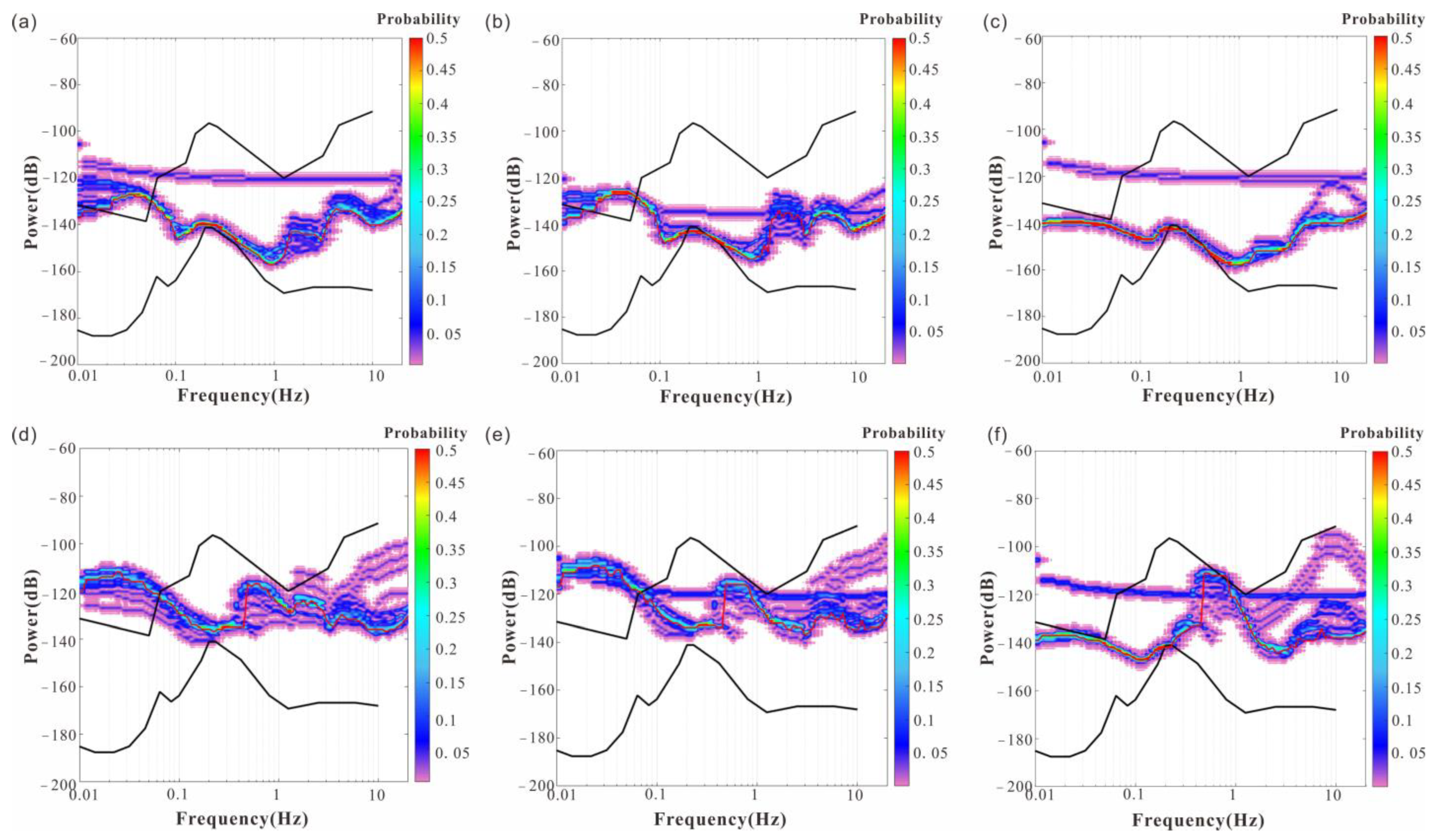
To verify the authenticity of the ambient noise data from the OBS at station B99 and better analyze the ambient noise level in the Arctic Chukchi Sea area, it is compared with station C15, which has a greater water depth but is located at a certain distance. In
Figure 3 and
Figure 4, apart from the linear distribution phenomenon caused by the seabed seismograph instrument itself, the range and trend of ambient noise at station C15 are approximately equal to those at station B99, lying between the values of NHNM and NLNM. However, there are some differences: since station C15 is farther from the coast and has a deeper deployment depth than station B99, there is less interference from very-low-frequency waves, resulting in a lower distribution of PSD in the long-period band for ambient noise. Additionally, by comparing the mode curve lines of the PSD for part A and part B (shown in
Figure 5), it can be observed that strong wind waves mainly affect the long-period band and microseismic band, with the frequency range of influence primarily distributed between 0.6 Hz and 6 Hz.
To gain a better understanding of the distribution of ambient noise power density in the Arctic, we calculated the PSD for all seismic records continuously observed by the B99 seismic station in the Chukchi Sea area. By obtaining the mode curve line of its PSD, we can compare it with other seismic stations for analysis. For this comparative analysis, we selected an inland China seismic station, a South China Sea OBS, and a Pacific OBS, all of which captured ambient noise.
We discovered that the ambient noise line in the Arctic is higher than that of the inland seismic station but lower than the levels observed in the South China Sea and the Pacific seafloor ambient noise. Arctic ambient noise lies in the transitional stage between mainland and marine ambient noise.
Figure 4 illustrates that the trend of ambient noise in the Chukchi Sea aligns closely with the underwater ambient noise in the South China Sea within the range of 0.085 Hz~0.2 Hz. Notably, there is no remote double-frequency microseism (DFM) observed within this frequency range. This absence of remote energy influence can be explained by the fact that both the South China Sea and Chukchi Sea are located at the edges of the ocean.
Furthermore, the ambient noise level in the Chukchi Sea is approximately 10 dB lower than that in the South China Sea overall. This difference can be attributed to the presence of sea ice in the Chukchi Sea, which acts as a shield and suppresses noise. A comparison with ambient noise at the Pacific Ocean OBS reveals distinct characteristics. The Pacific station exhibits two peaks in DFM: 2–5 s and 5–10 s, corresponding to different energy sources—local and remote. In contrast, the DFM in the Chukchi Sea experiences a rapid decline after 5 s, indicating that the marginal sea of the Chukchi Sea differs from the open ocean. The influence of the distant DFM is minimal, and the circulation characteristics of the Chukchi Sea itself play a significant role in its DFM. It is evident that local sources primarily contribute to the occurrence of DFM in the Chukchi Sea, which aligns with the results of the above analysis [
1,
46].
4. Emergency Ambient Noise Analysis
The PDF statistical method involves performing the same statistical processing on all data. The occurrence of low-probability events does not affect the results. In the calculation process, it is not necessary to exclude emergencies, such as earthquakes, or to deliberately extract periods with low external noise to calculate the PSD. Therefore, earthquakes and other aperiodic sudden noise are present in the distribution of the final statistical results as low-probability events.
To study the influence of sudden interference on ambient noise in a certain time period, we select the anomalous curve in the observational period to summarize noise.
4.1. Power Spectrum Anomaly Caused by a Strong Earthquake
When a significant earthquake occurs, the PSD noticeably differs from the noise observed during calm conditions.
Table 3 illustrates the PSD and corresponding waveforms for strong earthquake events at two different locations. Within the frequency range of 0~6 Hz, most frequencies surpass the NHNM values, except for a few frequencies that are lower than the NLNM values. The peak value is approximately 5 Hz, reaching −85 dB (as shown in
Figure 6). As the epicenter distance increases to 23.47°, the high-frequency energy of event ‘S2’ diminishes during propagation. The spectral characteristics above 3 Hz closely align with the noise pattern observed during calm conditions, while the long-period anomaly becomes evident.
Overall, strong earthquakes lead to significant fluctuations in the long-period curve, resulting in a decrease in the abnormal amplitude of the power spectrum curve as a whole. The peak value reaches −100 dB, exerting a substantial impact on the microseismic and high-frequency bands.
4.2. Power Spectrum Anomaly Caused by Small and Medium Earthquakes
The energy released by medium- and small-magnitude earthquakes is relatively weak, and the development of surface waves is not prominent (as shown in
Figure 7).
Table 4 provides an earthquake catalog for reference. The predominant frequencies of the three events are concentrated between 1 Hz and 10 Hz. Event ‘S3′ exhibits a peak value of approximately −118 dB, falling within the range of calm conditions. As the epicentral distance decreases and the magnitude increases, the overall anomalous curve for event ‘S4′ shows a substantial increase and reaches the peak value of ‘S3′ at approximately 5 Hz, reaching approximately −95 dB. Event ‘S5′ has an epicentral distance equivalent to that of ‘S4′, but it has a shallower focal depth and a slightly weaker spectral density between 0.3 Hz and 3 Hz compared to ‘S4′. Additionally, the frequency band is slightly narrower for ‘S5′.
By analyzing the power spectrum anomalies resulting from strong earthquakes as well as medium and small earthquakes, we observe that both types of earthquakes have substantial effects on the microseismic and high-frequency bands of Arctic marine ambient noise. As the epicentral distance increases, the impact of both strong and medium-to-small earthquakes becomes more pronounced. Moreover, we note that earthquakes with smaller magnitudes and shallower focal depths exhibit lower PSD values and narrower bandwidths.
5. Discussion
5.1. Error Norm Analysis
Error norm analysis methods are often used in the field of engineering geology, and error norms are defined as random errors [
47,
48,
49,
50]:
where
represents the error norm, and
and
represent the measured data of ambient noise on the seabed in the Chukchi Sea and the numerical magnitude predicted by each empirical formula, respectively. The relative error norm was introduced to reduce the error generated by the error norm itself under the same conditions. The relative error norm is defined as follows [
50,
51]:
Sensitivity analysis is a quantitative approach that assesses the degree of influence on another factor or group of factors when one variable changes. The practical application of sensitivity analysis involves using mathematical methods to incrementally or decrementally modify one variable and then calculate the resulting impact on another factor.
5.2. Analysis of Influence Factors on Ambient Noise Level
We observed the PSD of effective information over a period of 32 days, generating noise PSD data across time and frequency.
Figure 8 displays the three-component PSD time chart of effective information recorded at station B99 for 28 consecutive days (5 August to 1 September 2018), aiming to accurately observe the change in ambient noise within the Chukchi Sea area.
The noise PSD at station B99 exhibits similar variations, with a high ambient noise level in the long-period frequency band, indicating an active noise environment in the area. Notably, the vertical component noise shows minimal temporal changes in the long-period frequency band, whereas the microseismic frequency band experiences significant fluctuations over time. It is evident from the graph that there is a noticeable increase in the ambient noise level around the 10th to 11th day. This suggests that natural factors may influence ambient noise in the microseismic belt.
To investigate this further, we obtained sea ice concentration, wind speed, and significant wave height data from the location where the seabed seismograph was deployed between 3 August and 4 September 2018. We plotted the corresponding change curve, as shown in
Figure 8. To gain a deeper understanding of the impact of natural factors on the background ambient noise level in the Chukchi Sea area, this study utilizes the two-parameter equation method for further analysis.
The two-parameter equation has been previously employed to study the acoustic properties of sediments on the seafloor. This approach is utilized to address the limitations of single-parameter equations by establishing a connection between two parameters. Importantly, there should be no direct correlation between the two physical quantities in the calculation of the two-parameter equation. Hence, when developing a prediction equation for seafloor environment noise levels, including more parameters does not necessarily yield better results. In this study, we observe that wind speed and significant wave height exhibit a positive correlation (as shown in
Figure 9a), while there is no direct correlation between sea ice concentration and significant wave height (as shown in
Figure 9b). Therefore, this paper focuses on establishing a two-parameter equation that relates significant wave height, sea ice concentration, and ambient noise levels on the seabed. The significant wave height serves as an indicator of sea surface calmness, while sea ice concentration reflects the coverage of sea ice in a specific area. Based on the available data, a two-parameter equation relating significant wave height, sea ice concentration, and seabed ambient noise is formulated:
The two-parameter equation for seabed ambient noise level is represented by N, I, and W, where N denotes the noise level, I represents the sea ice concentration, and W represents the significant wave height. To perform sensitivity analysis on the two-parameter equation, mathematical methods are employed to modify one variable while keeping the other constant. This allows us to evaluate the sensitivity of the changed parameter on the equation’s outcome. By separately changing the input values of the two parameters and comparing their sensitivities, the order of sensitivity between the two parameters can be determined.
During sensitivity analysis, one parameter in the two-parameter equation is modified while the other remains unchanged. The input value of the unaltered parameter is held constant, and the input value of the modified parameter is adjusted incrementally or decrementally. The actual measured value is multiplied by a scaling factor ranging from 0 to 1, where a normalized value of 1 corresponds to the actual measured value. The parameter is then multiplied by a scaling factor ranging from 1 to 2, effectively expanding the parameter’s value range to 0–2. Finally, the modified parameter is used in the two-parameter equation, while the other parameter remains constant, resulting in a set of predicted values.
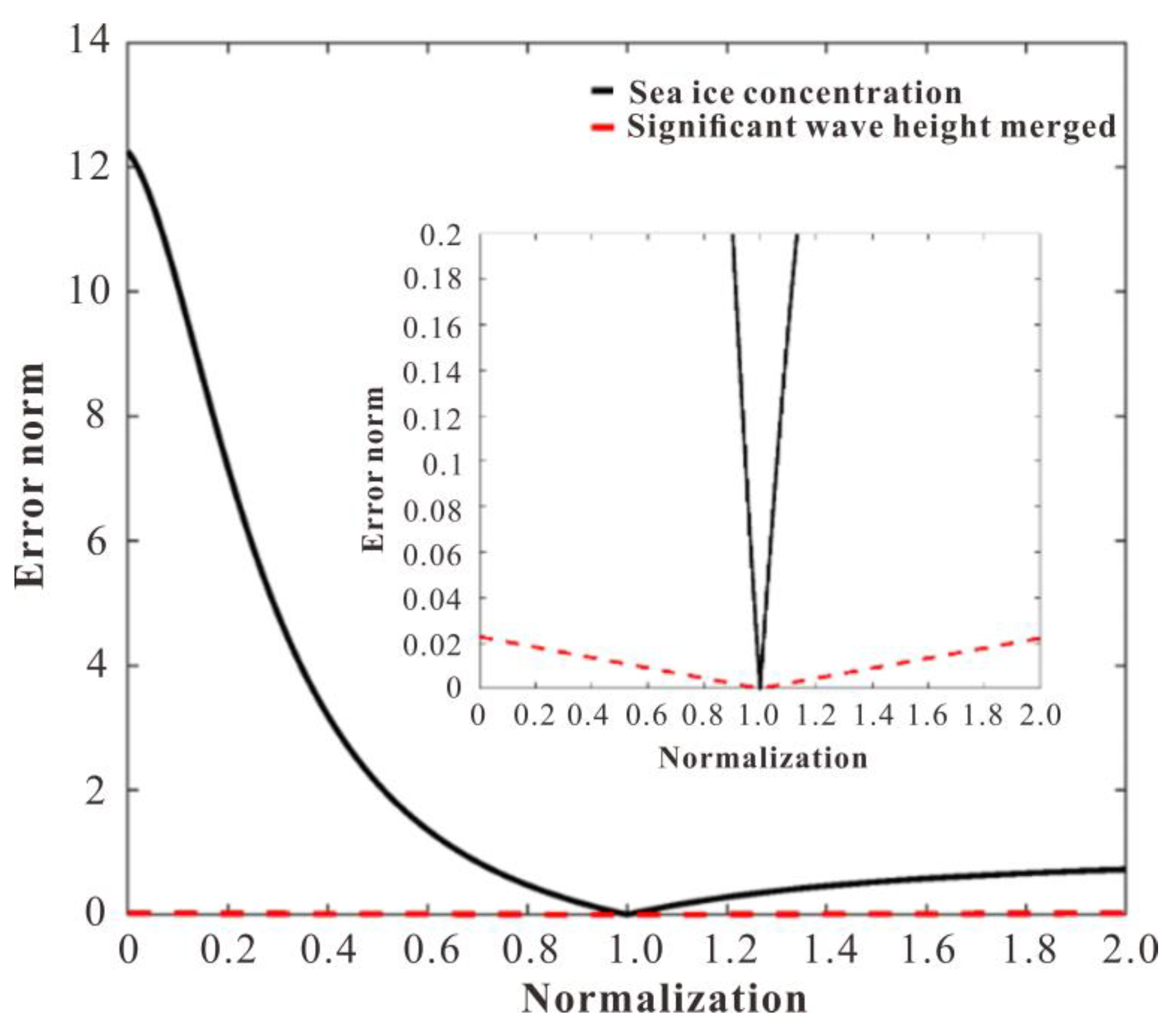
Error norm analysis was conducted on the two-parameter equation involving sea ice concentration and significant wave height, and a sensitivity analysis graph was generated (shown in
Figure 10). The analysis revealed that the sensitivity of sea ice concentration is significantly greater than that of significant wave height. In the larger plot, the relative error norm analysis of sea ice concentration demonstrates that within the range of 0–1, the relative error reaches values of 12 or more. However, the relative error norm decreases rapidly until it reaches 0 within this range. In the range of 1–2, the relative error norm analysis slowly rises to approximately 0.6, exhibiting a notable difference from the 0–1 range. On the other hand, the relative error norm of the significant wave height remains almost unchanged, consistently close to 0. When magnified, the relative error norm of the significant wave height forms a “V” shape with a gradual decrease from 0 to 1, followed by a slight increase up to 2. However, the maximum value does not exceed 0.02.
Based on the error norm analysis, we can conclude that within the two-parameter equation of sea ice concentration/significant wave height/seabed ambient noise level, the influence of sea ice concentration on predicting seabed ambient noise is much greater than the effect of significant wave height within the range of 0–1. In the range of 1–2, the impact of sea ice concentration on ambient noise prediction significantly diminishes but still surpasses the influence of significant wave height on seabed ambient noise prediction.
6. Conclusions
Based on the data recorded by seafloor seismographs at Chukchi Sea stations within the Arctic region, an analysis of ambient noise in the Chukchi Sea area was conducted using power density analysis and probability density function statistical analysis.
In the Arctic Chukchi Sea station area, the presence of sea ice on the sea surface plays a role in attenuating the noise caused by wind. Overall, the noise environment in the Arctic Chukchi Sea station area falls between the ambient noise levels observed in non-high latitude marine areas and global land areas. This suggests that the seismic signals received by ocean bottom seismometers are inferior to those obtained by land-based seismic stations.
The ambient noise in the Chukchi Sea does not exhibit remote double-frequency microseismic peaks in the microseismic frequency band. The occurrence of double-frequency peaks is primarily influenced by local sources. This is because the Chukchi Sea, being a marginal sea of the Arctic Ocean, experiences minimal impact from distant double-frequency microseisms. Instead, the circulation characteristics of the Chukchi Sea itself, which involve local sources, are the primary drivers of double-frequency microseism production.
Earthquakes cause a wide range of changes in the power spectrum, with low-frequency anomalies being particularly prominent during strong earthquakes. The bandwidth of these anomalies decreases as the epicenter distance increases. Small- and medium-sized earthquakes exhibit noticeable anomalies in the high-frequency range above 1 Hz.
Sea ice concentration significantly affects the ambient noise level in the Arctic sea area. Higher sea ice concentrations correspond to lower ambient noise levels at the seafloor. As sea ice concentration decreases, the noise shielding effect on the seafloor diminishes, and the influence of wind speed and significant wave height on the ambient noise level becomes more pronounced.
Due to the high-latitude location of the Arctic, the deployment and retrieval of seafloor seismographs are limited by climatic conditions, environmental factors, and other constraints. Therefore, this paper presents only the 30-day effective signal, draws the PSD distribution map of ambient noise in the Chukchi Sea area, and briefly introduces the ambient noise source in the Chukchi Sea area. However, there is no systematic research and analysis on the seasonal and annual variations in ambient noise in the Chukchi Sea area, which will be the direction for our future research.


 ,
, 


