

A Robust Adaptive Extended Kalman Filter Based on an Improved Measurement Noise Covariance Matrix for the Monitoring and Isolation of Abnormal Disturbances in GNSS/INS Vehicle Navigation

Abstract
:
1. Introduction
2. Materials and Methods
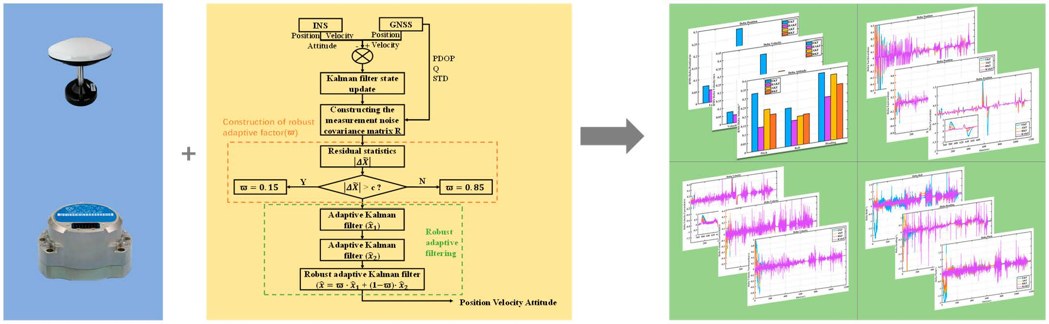
2.1. Steps of the Improved Robust Adaptive Factor Method
2.2. Classical GNSS/INS Loosely Coupled Integrated Procedure
2.3. Robust Adaptive Filtering Algorithm with Improved Measurement Noise Covariance Matrix
2.3.1. Construction of the Improved Measurement Noise Covariance Matrix
2.3.2. Robust Adaptive Filtering Construction
- Calculate the gain matrix: ;
- Calculate the state estimate at time k: ;
- Calculate the estimate error covariance matrix at time k: .
- Calculate the gain matrix: ;
- Calculate the state estimate at time k: ;
- Calculate the estimate error covariance matrix at time k: .
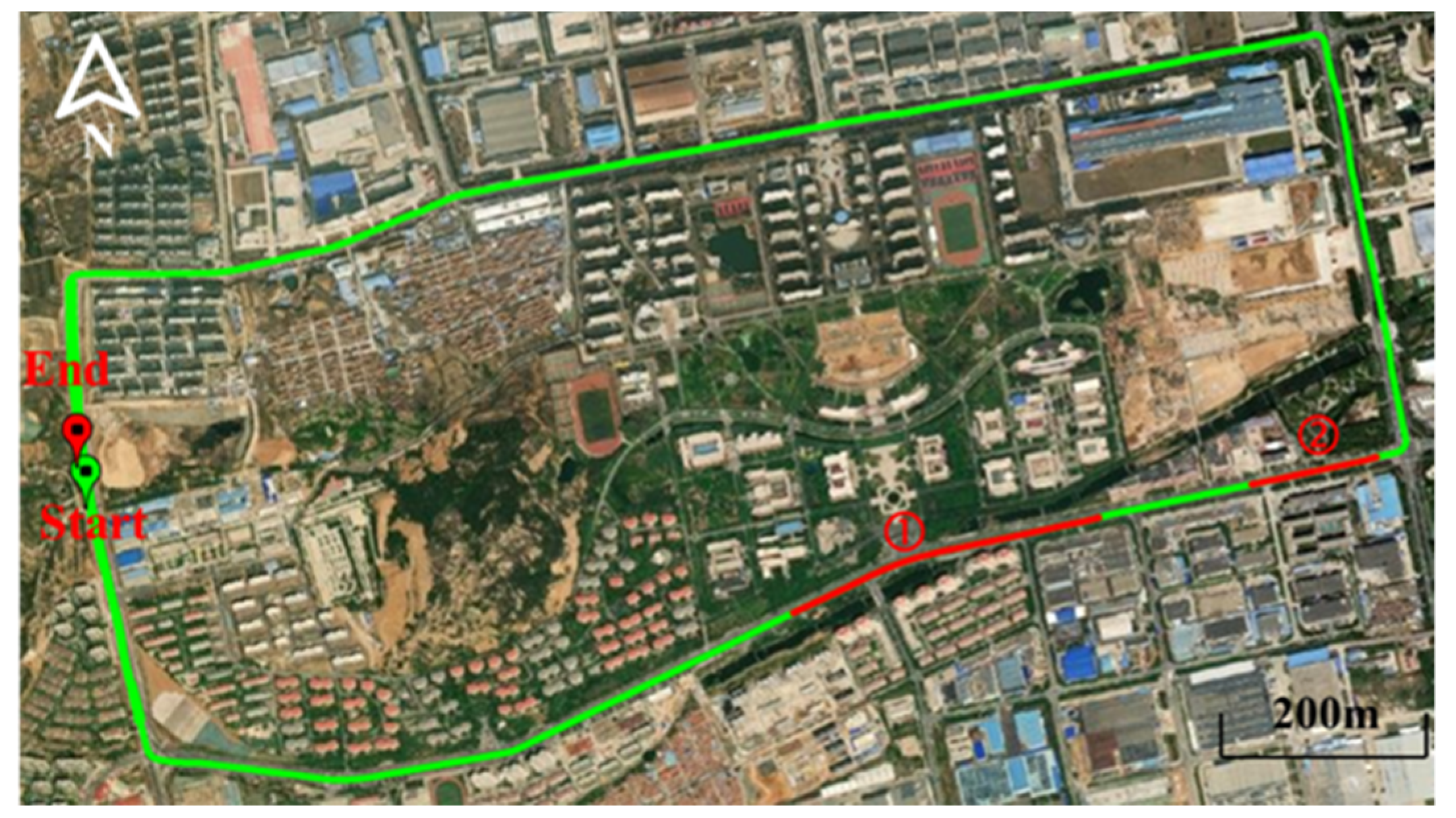
2.4. Datasets and Processing Strategies
3. Results
3.1. Experimental Results for the Measurement Noise Covariance Matrix
3.2. Vehicle Experimental Results
3.2.1. Vehicle Experimental 1 Results
- Regarding position error: In terms of the East–North–Up (ENU) position error, compared with EKF, the accuracy of RAKF increased by 27.03%, 77.92%, and 72.56%, respectively. Compared with AKF, the accuracy of RAKF improved by 2.84% and 10.85%, respectively. Compared with RKF, the accuracy of RAKF improved by 22.62%, 51.79%, and 54.19%, respectively. In the position average accuracy, compared with the three algorithms, the accuracy of RAKF improved by 72.43%, 2.54%, and 47.82%, respectively.
- Regarding velocity error: In terms of the East–North–Up (NEU) velocity error, compared with EKF, the accuracy of RAKF increased by 31.34%, 86.04%, and 26.44%, respectively. Compared with AKF, the accuracy of RAKF improved by 34.27% and 77.58%, respectively. Compared with RKF, the accuracy of RAKF improved by 29.57%, 79.91%, and 2.93%, respectively.
- Regarding attitude errors: In terms of the pitch–roll–heading–attitude error, compared with EKF, the accuracy of RAKF increased by 59.54%, 34.08%, and 35.85%, respectively. Compared with AKF, the accuracy of RAKF improved by 41.91%, 12.44%, and 32.79%, respectively. Compared with RKF, the accuracy of RAKF improved by 32.31%, 15.54%, and 19.86%, respectively.
3.2.2. The Comparison Results of the Single GPS System and GPS+GLONASS+BDS Three Systems
3.2.3. Vehicle Experiment 2 Results
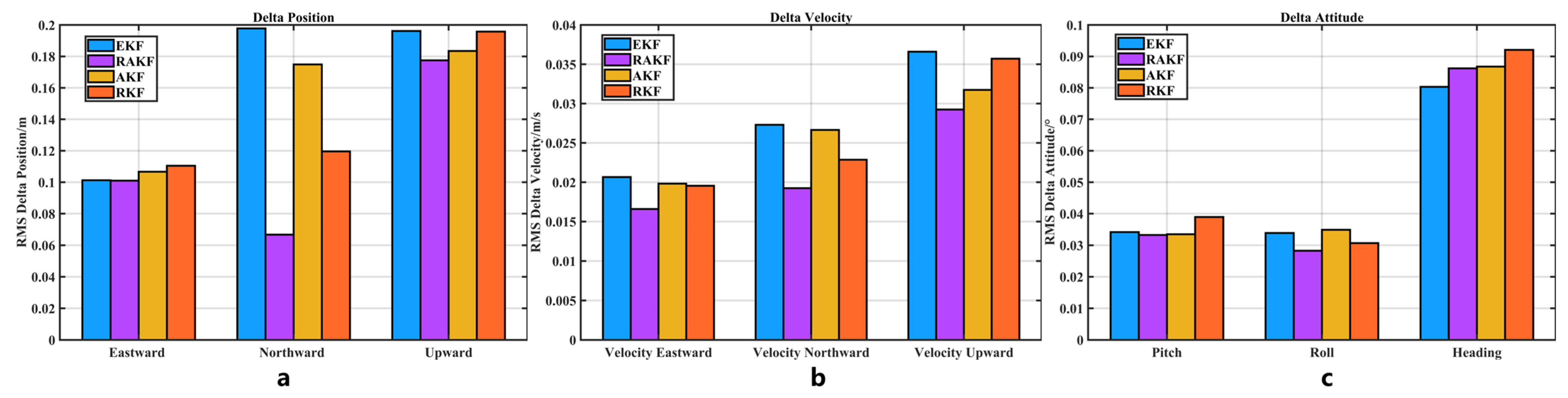
- Regarding position error: In terms of the East–North–Up (ENU) position error, compared with EKF, the accuracy of RAKF increased by 0%, 66.28%, and 9.53%, respectively. Compared with AKF, the accuracy of RAKF improved by 5.34% and 64.86%, and 3.22%, respectively. Compared with RKF, the accuracy of RAKF improved by 8.24%, 44.23%, and 9.35%, respectively. In the position average accuracy, compared with the three algorithms, the accuracy of RAKF improved by 27.53%, 21.89%, and 15.63%, respectively.
- Regarding velocity error: In terms of the East–North–Up (ENU) velocity error, compared with EKF, the accuracy of RAKF increased by 19.81%, 29.67%, and 20.22%, respectively. Compared with AKF, the accuracy of RAKF improved by 16.16%, 27.82%, and 7.89%, respectively. Compared with RKF, the accuracy of RAKF improved by 14.87%, 16.16%, and 18.21%, respectively.
3.3. Add Different Disturbance Vehicle Experiment Results
3.3.1. Experimental Results of the First Group
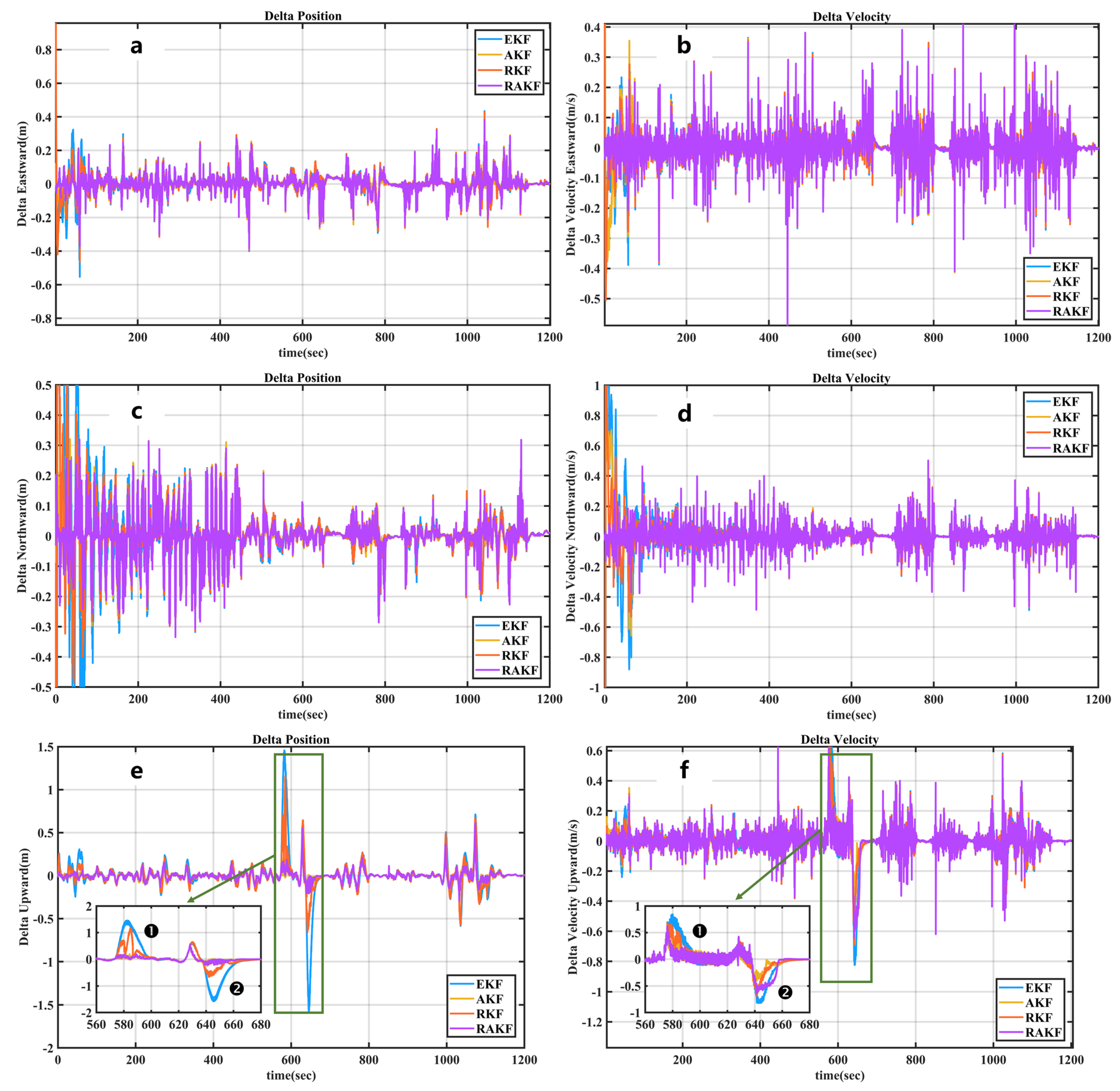
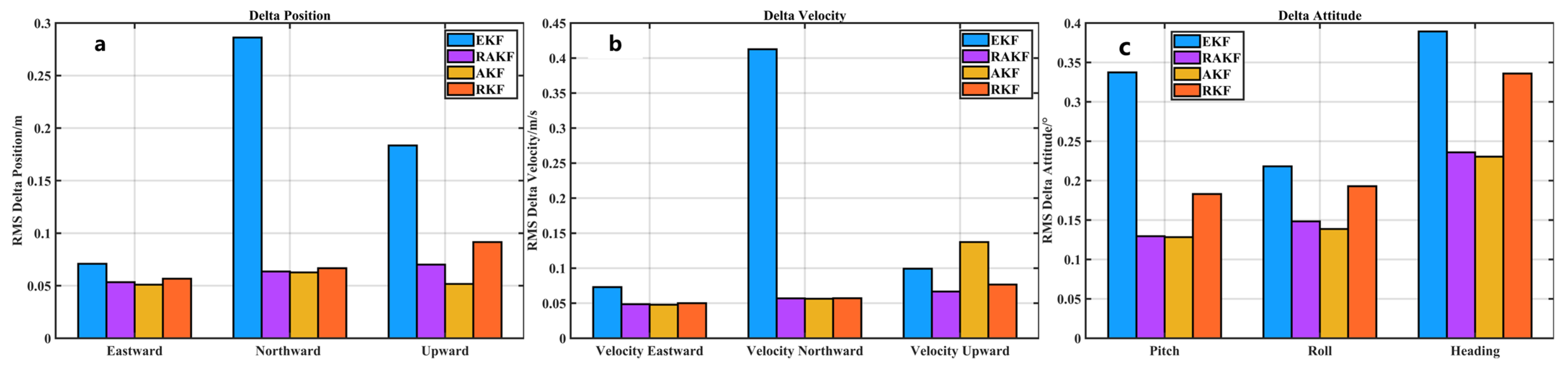
- Regarding position error: When adding 1-s random disturbances ranging from 0 to 1 m, in terms of the East–North–Up (ENU) position error, compared with EKF, the accuracy of RAKF increased by 24.89%, 77.78%, and 68.79%, respectively. Compared to RKF, the accuracy of RAKF achieved improvements of 20.36%, 77.78%, and 68.79%, respectively. Figure 17a–c illustrates the comparison of position errors with 1-s disturbances ranging from 0 to 1 m. In this scenario, the RAKF algorithm outperformed RKF significantly. Compared to EKF and AKF, RAKF demonstrated comparable anti-interference capability but with slightly better performance and closer proximity to 0.
- Regarding velocity error: When adding 1-s random disturbances ranging from 0 to 1 m, in terms of the East–North–Up (ENU) velocity error, compared with EKF, the accuracy of RAKF improved by 31.20%, 86.04%, and 41.88%, respectively. Compared with AKF, the accuracy of RAKF improved by 34.13%, 77.58%, and 7.54%, respectively. Compared with RKF, the speed accuracy of RAKF improved by 29.43%, 79.91%, and 23.30%, respectively.
- Regarding attitude error: When adding 1-s random disturbances ranging from 0 to 1 m, in terms of the pitch, roll, heading, and attitude error, compared with EKF, the accuracy of RAKF improved by 59.38%, 30.15%, and 34.65%, respectively. Compared with AKF, the accuracy of RAKF improved by 14.18%, 7.21%, and 31.53%, respectively. Compared with RKF, the accuracy of RAKF improved by 32.06%, 10.50%, and 18.36%, respectively.
3.3.2. Experimental Results of the Second Group
4. Discussion
5. Conclusions
Author Contributions
Funding
Data Availability Statement
Acknowledgments
Conflicts of Interest
References
- Yang, Y.; Yang, C.; Ren, X. PNT intelligent services. Acta Geod. Et Cartogr. Sin. 2021, 50, 1006–1012. [Google Scholar] [CrossRef]
- Yang, Y. Resilient PNT Concept Frame. Acta Geod. Et Cartogr. Sin. 2018, 47, 893–898. [Google Scholar] [CrossRef]
- Filjar, R.; Damas, M.C.; Iliev, T.B. Resilient Satellite Navigation Empowers Modern Science, Economy, and Society. IOP Conf. Ser. Mater. Sci. Eng. 2021, 1032, 012001. [Google Scholar] [CrossRef]
- Fritsche, M.; Sośnica, K.; Rodríguez-Solano, C.J.; Steigenberger, P.; Wang, K.; Dietrich, R.; Dach, R.; Hugentobler, U.; Rothacher, M. Homogeneous Reprocessing of GPS, GLONASS and SLR Observations. J. Geod. 2014, 88, 625–642. [Google Scholar] [CrossRef]
- Zhang, B.; Hou, P.; Zha, J.; Liu, T. Integer-Estimable FDMA Model as an Enabler of GLONASS PPP-RTK. J. Geod. 2021, 95, 91. [Google Scholar] [CrossRef]
- Paziewski, J.; Wielgosz, P. Assessment of GPS + Galileo and Multi-Frequency Galileo Single-Epoch Precise Positioning with Network Corrections. GPS Solut. 2014, 18, 571–579. [Google Scholar] [CrossRef]
- Qu, L.; Du, M.; Wang, J.; Gao, Y.; Zhao, Q.; Zhang, Q.; Guo, X. Precise Point Positioning Ambiguity Resolution by Integrating BDS-3e into BDS-2 and GPS. GPS Solut. 2019, 23, 63. [Google Scholar] [CrossRef]
- Chai, D.; Sang, W.; Chen, G.; Ning, Y.; Xing, J.; Yu, M.; Wang, S. A Novel Method of Ambiguity Resolution and Cycle Slip Processing for Single-Frequency GNSS/INS Tightly Coupled Integration System. Adv. Space Res. 2022, 69, 359–375. [Google Scholar] [CrossRef]
- Hu, L.; Bao, Y.; Sun, Z.; Meng, X.; Tang, C.; Zhang, D. Outlier Detection Based on Nelder-Mead Simplex Robust Kalman Filtering for Trustworthy Bridge Structural Health Monitoring. Remote Sens. 2023, 15, 2385. [Google Scholar] [CrossRef]
- Feng, S.; Ochieng, W.; Moore, T.; Hill, C.; Hide, C. Carrier Phase-Based Integrity Monitoring for High-Accuracy Positioning. GPS Solut. 2009, 13, 13–22. [Google Scholar] [CrossRef]
- Jiang, C.; Zhao, D.; Zhang, Q.; Liu, W. A Multi-GNSS/IMU Data Fusion Algorithm Based on the Mixed Norms for Land Vehicle Applications. Remote Sens. 2023, 15, 2439. [Google Scholar] [CrossRef]
- Cheng, S.; Cheng, J.; Zang, N.; Cai, J.; Fan, S.; Zhang, Z.; Song, H. Adaptive Non-Holonomic Constraint Aiding Multi-GNSS PPP/INS Tightly Coupled Navigation in the Urban Environment. GPS Solut. 2023, 27, 152. [Google Scholar] [CrossRef]
- Chai, D.; Chen, G.; Wang, S.; Lu, X. Loosely Coupled GNSS/INS Integration Based on an Auto Regressive Model in a Data Gap Environment. Acta Geod. Geophys. 2018, 53, 691–715. [Google Scholar] [CrossRef]
- Xiao, Y.; Luo, H.; Zhao, F.; Wu, F.; Gao, X.; Wang, Q.; Cui, L. Residual Attention Network-Based Confidence Estimation Algorithm for Non-Holonomic Constraint in GNSS/INS Integrated Navigation System. IEEE Trans. Veh. Technol. 2021, 70, 11404–11418. [Google Scholar] [CrossRef]
- Musoff, H.; Zarchan, P. Fundamentals of Kalman Filtering: A Practical Approach, 3rd ed.; American Institute of Aeronautics and Astronautics: Reston, VA, USA, 2009; ISBN 978-1-60086-718-7. [Google Scholar]
- Zhang, B.; Hou, P.; Liu, T.; Yuan, Y. A Single-Receiver Geometry-Free Approach to Stochastic Modeling of Multi-Frequency GNSS Observables. J. Geod. 2020, 94, 37. [Google Scholar] [CrossRef]
- Chen, G. Introduction to random signals and applied Kalman filtering, 2nd edn. Robert Grover Brown and Patrick Y. C. Hwang, Wiley, New York, 1992. ISBN 0-471-52573-1, 512 pp., $62.95. Int. J. Adapt. Control. Signal Process. 1992, 6, 516–518. [Google Scholar] [CrossRef]
- Ding, W.; Wang, J.; Rizos, C.; Kinlyside, D. Improving Adaptive Kalman Estimation in GPS/INS Integration. J. Navig. 2007, 60, 517–529. [Google Scholar] [CrossRef]
- Yan, W.; Bastos, L.; Gonçalves, J.A.; Magalhães, A.; Xu, T. Image-Aided Platform Orientation Determination with a GNSS/Low-Cost IMU System Using Robust-Adaptive Kalman Filter. GPS Solut. 2018, 22, 12. [Google Scholar] [CrossRef]
- Liu, S.; Wang, K.; Abel, D. Robust State and Protection-Level Estimation within Tightly Coupled GNSS/INS Navigation System. GPS Solut. 2023, 27, 111. [Google Scholar] [CrossRef]
- Huang, Y.; Zhang, Y.; Wu, Z.; Li, N.; Chambers, J. A Novel Adaptive Kalman Filter With Inaccurate Process and Measurement Noise Covariance Matrices. IEEE Trans. Automat. Contr. 2018, 63, 594–601. [Google Scholar] [CrossRef]
- Mohamed, A.H.; Schwarz, K.P. Adaptive Kalman Filtering for INS/GPS. J. Geod. 1999, 73, 193–203. [Google Scholar] [CrossRef]
- Wang, J. Stochastic Modeling for Real-Time Kinematic GPS/GLONASS Positioning. Navigation 1999, 46, 297–305. [Google Scholar] [CrossRef]
- Hide, C.; Moore, T.; Smith, M. Adaptive Kalman Filtering for Low-Cost INS/GPS. J. Navig. 2003, 56, 143–152. [Google Scholar] [CrossRef]
- Meng, Y.; Gao, S.; Zhong, Y.; Hu, G.; Subic, A. Covariance Matching Based Adaptive Unscented Kalman Filter for Direct Filtering in INS/GNSS Integration. Acta Astronaut. 2016, 120, 171–181. [Google Scholar] [CrossRef]
- Yang, Y.; He, H.; Xu, G. Adaptively Robust Filtering for Kinematic Geodetic Positioning. J. Geod. 2001, 75, 109–116. [Google Scholar] [CrossRef]
- Gao, S.; Zhong, Y.; Li, W. Robust Adaptive Filtering Method for SINS/SAR Integrated Navigation System. Aerosp. Sci. Technol. 2011, 15, 425–430. [Google Scholar] [CrossRef]
- Niu, X.; Wu, J.; Zhang, Q. Research on Measurement Error Model of GNSS/INS Integration Based on Consistency Analysis. Gyroscopy Navig. 2018, 9, 243–254. [Google Scholar] [CrossRef]
- Niu, X.; Dai, Y.; Liu, T.; Chen, Q.; Zhang, Q. Feature-Based GNSS Positioning Error Consistency Optimization for GNSS/INS Integrated System. GPS Solut. 2023, 27, 89. [Google Scholar] [CrossRef]
- Crespillo, O.G.; Medina, D.; Skaloud, J.; Meurer, M. Tightly coupled GNSS/INS integration based on Robust M-Estimators. In Proceedings of the 2018 IEEE/ION Position, Location and Navigation Symposium (PLANS), Portland, OR, USA, 20–23 April 2020; IEEE: Monterey, CA, USA; pp. 1554–1561. [Google Scholar]
- Yang, Y. Adaptive Dynamic Navigation and Positioning; Surveying and Mapping Press: Beijing, China, 2017; ISBN 978-7-5030-4005-4. [Google Scholar]
- Mao, Y.; Sun, R.; Wang, J.; Cheng, Q.; Kiong, L.C.; Ochieng, W.Y. New Time-Differenced Carrier Phase Approach to GNSS/INS Integration. GPS Solut. 2022, 26, 122. [Google Scholar] [CrossRef]
- Wen, W.; Kan, Y.C.; Hsu, L.-T. Performance comparison of GNSS/INS integrations based on EKF and factor graph optimization. In Proceedings of the 32nd International Technical Meeting of the Satellite Division of The Institute of Navigation (ION GNSS+ 2019), Miami, FL, USA, 16–20 September 2019; pp. 3019–3032. [Google Scholar]
- Yan, G.; Weng, J. Integrated Inertial Navigation Algorithms and Principles of Integrated Navigation; Northwestern Polytechnical University: Xi’an, China, 2019; ISBN 978-7-5612-6547-5. [Google Scholar]
- Jiang, C. Filtering algorithms and reliability analysis for GNSS/INS integrated navigation systems. Acta Geod. Et Cartogr. Sin. 2020, 49, 1376. [Google Scholar] [CrossRef]
- Yang, Y.; Ren, X.; Xu, Y. Main Process of Adaptively Robust Filter with Applications in Navigation. J. Navig. Position. 2013, 1, 9–15. [Google Scholar] [CrossRef]
- Jiang, C.; Zhang, S.; Li, H.; Li, Z. Performance Evaluation of the Filters with Adaptive Factor and Fading Factor for GNSS/INS Integrated Systems. GPS Solut. 2021, 25, 130. [Google Scholar] [CrossRef]
- Knight, N.L.; Wang, J. A Comparison of Outlier Detection Procedures and Robust Estimation Methods in GPS Positioning. J. Navig. 2009, 62, 699–709. [Google Scholar] [CrossRef]
- Niu, Z.; Li, G.; Guo, F.; Shuai, Q.; Zhu, B. An Algorithm to Assist the Robust Filter for Tightly Coupled RTK/INS Navigation System. Remote Sens. 2022, 14, 2449. [Google Scholar] [CrossRef]
- Akhlaghi, S.; Zhou, N.; Huang, Z. Adaptive adjustment of noise covariance in Kalman filter for dynamic state estimation. In Proceedings of the IEEE Power Energy Society General Meeting, Chicago, IL, USA, 16–20 July 2017; pp. 1–5. [Google Scholar] [CrossRef]


| Measurement Factor (Q) | Description | 3D Accuracy (m) |
|---|---|---|
| 1 | Fixed integer | 0.00–0.15 |
| 2 | Converged float or noise Fixed integer | 0.05–0.40 |
| 3 | Converging float | 0.2–1.0 |
| 4 | Converging float | 0.5–2.00 |
| 5 | DGPS | 1.00–5.00 |
| 6 | DGPS | 2.00–10.00 |
| Gyroscopes | Accelerometers | |
|---|---|---|
| Bias | 0.25°/h | 0.025°/h |
| Random noise | 0.04°/sqrt(h) | 0.03m/s/sqrt(h) |
| Method | R |
|---|---|
| 1 | |
| 2 | |
| 3 | |
| 4 | |
| 5 | |
| 6 | |
| 7 |
| Mode | PE (m) | PN (m) | PU (m) | VE (m/s) | VN (m/s) | VU (m/s) | Pitch (°) | Roll (°) | Yaw (°) |
|---|---|---|---|---|---|---|---|---|---|
| EKF | 0.0703 | 0.2867 | 0.1833 | 0.0718 | 0.4025 | 0.0991 | 0.3230 | 0.2136 | 0.3824 |
| 1 | 0.0509 | 0.0632 | 0.0508 | 0.0482 | 0.0555 | 0.1001 | 0.1287 | 0.1404 | 0.2514 |
| 2 | 0.0514 | 0.0632 | 0.0542 | 0.0486 | 0.0558 | 0.0982 | 0.1301 | 0.1378 | 0.2453 |
| 3 | 0.0512 | 0.0631 | 0.0529 | 0.0484 | 0.0557 | 0.0729 | 0.1307 | 0.1408 | 0.2453 |
| 4 | 0.0513 | 0.0633 | 0.0503 | 0.0493 | 0.0562 | 0.0729 | 0.1307 | 0.1408 | 0.2409 |
| 5 | 0.0531 | 0.0639 | 0.0644 | 0.0497 | 0.0566 | 0.1052 | 0.1307 | 0.1377 | 0.2409 |
| 6 | 0.0520 | 0.0635 | 0.0607 | 0.0494 | 0.0563 | 0.0743 | 0.1295 | 0.1445 | 0.2406 |
| 7 | 0.0521 | 0.0638 | 0.0633 | 0.0495 | 0.0565 | 0.0793 | 0.1298 | 0.1419 | 0.2396 |
| Improved (%) | 26.65% | 77.92% | 72.56% | 31.34% | 86.04% | 26.44% | 59.54% | 33.57% | 37.00% |
| ERROR | EKF | AKF | RKF | RAKF | |
|---|---|---|---|---|---|
| Velocity (m/s) | Eastward | 0.0718 | 0.0750 | 0.0700 | 0.0493 |
| Northward | 0.4025 | 0.2507 | 0.2797 | 0.0562 | |
| Upward | 0.0991 | 0.0623 | 0.0751 | 0.0729 | |
| Attitude (deg) | Pitch | 0.3230 | 0.2250 | 0.1931 | 0.1307 |
| Roll | 0.2136 | 0.1608 | 0.1667 | 0.1408 | |
| Heading | 0.3824 | 0.3650 | 0.3061 | 0.2453 | |
| Position (m) | Eastward | 0.0703 | 0.0528 | 0.0663 | 0.0513 |
| Northward | 0.2867 | 0.0710 | 0.1313 | 0.0633 | |
| Upward | 0.1833 | 0.0428 | 0.1098 | 0.0503 | |
| 3D Accuracy(m) | 0.3475 | 0.0983 | 0.1836 | 0.0958 | |
| improved accuracy (%) | 72.43% | 2.54% | 47.82% | ||
| Eastward Error STD (m) | Northward Error STD (m) | Upward Error STD (m) | 3D Accuracy (m) | |
|---|---|---|---|---|
| Single GPS | 0.3059 | 0.5926 | 0.3148 | 0.7375 |
| Three systems | 0.0521 | 0.0643 | 0.0510 | 0.0972 |
| improved accuracy (%) | 82.97% | 89.15% | 83.80% | 86.82% |
| ERROR | EKF | AKF | RKF | RAKF | |
|---|---|---|---|---|---|
| Velocity (m/s) | Eastward | 0.0207 | 0.0198 | 0.0195 | 0.0166 |
| Northward | 0.0273 | 0.0266 | 0.0229 | 0.0192 | |
| Upward | 0.0366 | 0.0292 | 0.0317 | 0.0357 | |
| Attitude (deg) | Pitch | 0.0342 | 0.0335 | 0.0389 | 0.0333 |
| Roll | 0.0339 | 0.0349 | 0.0307 | 0.0283 | |
| Heading | 0.0803 | 0.0868 | 0.0921 | 0.0862 | |
| Position (m) | Eastward | 0.1013 | 0.1067 | 0.1104 | 0.1010 |
| Northward | 0.1978 | 0.1749 | 0.1196 | 0.0667 | |
| Upward | 0.1962 | 0.1834 | 0.1958 | 0.1775 | |
| 3D Accuracy(m) | 0.2964 | 0.2750 | 0.2546 | 0.2148 | |
| improved accuracy (%) | 27.53% | 21.89% | 15.63% | ||
| Experimental | Add Perturbation Time/s | Add Perturbation Value/m | Disturbance Duration/s |
|---|---|---|---|
| Group 1 | 368963 | 0.1576 | 1 |
| 0.9706 | |||
| 0.9572 | |||
| 0.4854 | |||
| 0.8003 | |||
| Group 2 | 369398 | 0.2721 | 1 |
| 369399 | 1.0997 | 1 | |
| 369400 | 1.1594 | 1 | |
| 369401 | 0.3380 | 1 | |
| 369402 | 0.2899 | 1 |
| ERROR | EKF | AKF | RKF | RAKF | |
|---|---|---|---|---|---|
| Velocity (m/s) | Eastward | 0.0729 | 0.0478 | 0.0500 | 0.0486 |
| Northward | 0.4126 | 0.0563 | 0.0570 | 0.0569 | |
| Upward | 0.0993 | 0.1372 | 0.0766 | 0.0666 | |
| Attitude (deg) | Pitch | 0.3373 | 0.1283 | 0.1830 | 0.1295 |
| Roll | 0.2181 | 0.1372 | 0.1930 | 0.1483 | |
| Heading | 0.3893 | 0.2304 | 0.3360 | 0.2359 | |
| Position (m) | Eastward | 0.0709 | 0.0510 | 0.0567 | 0.0534 |
| Northward | 0.2862 | 0.0626 | 0.0667 | 0.0635 | |
| Upward | 0.1835 | 0.0517 | 0.0915 | 0.0701 | |
| 3D Accuracy(m) | 0.3473 | 0.0959 | 0.1266 | 0.1086 | |
| improved accuracy (%) | 68.73% | - | 14.22% | ||
| ERROR | EKF | AKF | RKF | RAKF | |
|---|---|---|---|---|---|
| Velocity (m/s) | Eastward | 0.0782 | 0.0478 | 0.0493 | 0.0486 |
| Northward | 0.4575 | 0.0563 | 0.0565 | 0.0569 | |
| Upward | 0.1251 | 0.1375 | 0.0712 | 0.0666 | |
| Attitude (deg) | Pitch | 0.3858 | 0.1283 | 0.1387 | 0.1295 |
| Roll | 0.2377 | 0.1386 | 0.1633 | 0.1483 | |
| Heading | 0.4327 | 0.2304 | 0.3858 | 0.2359 | |
| Position (m) | Eastward | 0.0889 | 0.0510 | 0.0553 | 0.0534 |
| Northward | 0.4099 | 0.0626 | 0.0651 | 0.0635 | |
| Upward | 0.2914 | 0.0654 | 0.0981 | 0.0701 | |
| 3D Accuracy(m) | 0.5107 | 0.1039 | 0.1301 | 0.1086 | |
| improved accuracy (%) | 78.74% | - | 16.53% | ||
Disclaimer/Publisher’s Note: The statements, opinions and data contained in all publications are solely those of the individual author(s) and contributor(s) and not of MDPI and/or the editor(s). MDPI and/or the editor(s) disclaim responsibility for any injury to people or property resulting from any ideas, methods, instructions or products referred to in the content. |
© 2023 by the authors. Licensee MDPI, Basel, Switzerland. This article is an open access article distributed under the terms and conditions of the Creative Commons Attribution (CC BY) license (https://creativecommons.org/licenses/by/4.0/).
Share and Cite
Yin, Z.; Yang, J.; Ma, Y.; Wang, S.; Chai, D.; Cui, H. A Robust Adaptive Extended Kalman Filter Based on an Improved Measurement Noise Covariance Matrix for the Monitoring and Isolation of Abnormal Disturbances in GNSS/INS Vehicle Navigation. Remote Sens. 2023, 15, 4125. https://doi.org/10.3390/rs15174125
Yin Z, Yang J, Ma Y, Wang S, Chai D, Cui H. A Robust Adaptive Extended Kalman Filter Based on an Improved Measurement Noise Covariance Matrix for the Monitoring and Isolation of Abnormal Disturbances in GNSS/INS Vehicle Navigation. Remote Sensing. 2023; 15(17):4125. https://doi.org/10.3390/rs15174125
Chicago/Turabian StyleYin, Zhihui, Jichao Yang, Yue Ma, Shengli Wang, Dashuai Chai, and Haonan Cui. 2023. "A Robust Adaptive Extended Kalman Filter Based on an Improved Measurement Noise Covariance Matrix for the Monitoring and Isolation of Abnormal Disturbances in GNSS/INS Vehicle Navigation" Remote Sensing 15, no. 17: 4125. https://doi.org/10.3390/rs15174125