1. Introduction
The significant wave height (SWH) is the most important parameter characterizing surface waves, since the energy of sea waves is related to this parameter. The SWH is currently the only parameter of sea waves that is measured globally on a permanent basis. This information is assimilated into wave and Earth climate models. Since 1993, the SWH has been continuously measured throughout the world’s oceans using satellite radar altimeters [
1]. Traditionally, satellite radar altimeters for measuring SWH use an approach based on the analysis of the shape of the pulse reflected by the sea surface. The distance to the average level of the water surface is determined by the pulse delay time, and the SWH is measured using the slope of the leading edge of the pulse. This approach has been proven to work when validated and verified with wave buoy data. About 1500 such buoys are in the world’s oceans. Modern algorithms of satellite radar altimeters allow for achieving an accuracy of 3 cm for the average level of the water surface and 40 cm or 10%, whichever is greater, for the SWH. Also, an approach is now being developed to measure the average level of the water surface using antenna systems of radars with a spatial base [
2,
3,
4]. This approach is based on changing the phase difference of the reflected signal received on two antennas separated in space.
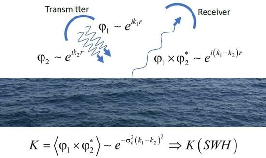
However, there is a fundamentally different approach, in which a two-frequency cross-correlation function of reflected signals is used to measure the SWH [
5,
6,
7]. For this method, it is necessary to transmit two signals at two close frequencies and receive reflection from the water surface of these two signals. Then, the correlation of the reflected signals is analyzed. This approach, in comparison with the traditional one for radar altimeters, potentially allows one to achieve higher measurement accuracy for weak waves. This effect is achieved by using different frequency bases to measure different ranges of SWH. The effectiveness of this approach has been confirmed in aircraft experiments [
8,
9]. The work in [
10] considers the extension of this approach to off-nadir sensing at small incidence angles. This opens up the possibility of measuring the SWH in the swath. The disadvantage of this approach is the complexity of use in satellite remote sensing. Because of this, for example, when analyzing the bistatically reflected navigation signal on satellites, the two-frequency cross-correlation function is used only to measure the water level [
11]. However, a solution was also proposed for satellite SWH measurement using antenna synthesis [
12,
13] in a monostatic problem statement.
At present, the bistatic problem statement is developing very actively in connection with the use of reflected signals from the Global Navigation Satellite Systems (GNSS) [
14] and other signals from various sources (Signals of Opportunity) [
15]. In the framework of bistatic radar measurements based on reflected GNSS signals and Signals of Opportunity, altimetry problems are solved, particularly measurements of the water surface level [
16] and SWH [
17,
18].
The bistatic problem statement has several advantages over the monostatic one. For example, in a bistatic measurement scheme, it is possible to carry out measurements at a distance from the transmitter and receiver and, at the same time, remain in the quasi-specular reflection region, which makes it possible to use more understandable formulas for describing reflection. The quasi-specular reflection region is also characterized by a high level of reflection power, which makes it possible to use this approach on small spacecraft to receive the signal of satellite navigation systems reflected by the Earth’s surface. In the region of resonant (Bragg) scattering of navigational signals, the reception of the reflected signal in orbit is impossible. In the bistatic problem statement, the analysis of the two-frequency cross-correlation function makes it possible to obtain an explicit relationship of the measured parameter with the wave parameters and the geometry of the problem. Such a formula for the reflected pulse in the bistatic problem statement has not been obtained to date.
In this paper, for the first time, we apply an approach based on the analysis of a two-frequency correlation function to measure SWH in a bistatic problem statement. The applicability of this approach is studied, including for satellite measurements. To do this, we obtain an expression for the modulus of the normalized cross-correlation function of two signals spaced in frequency in the quasi-specular reflection region. The problem is solved in Kirchhoff’s approximation, which makes it possible to accurately describe the reflection of microwave radiation by a water surface in the quasi-specular region. When deriving expressions, an independent choice of radiation patterns of the transmitting and receiving antennas is used, and it remains possible to set these patterns as asymmetric. In a previous work [
19], an expression for the cross-correlation function was obtained for the general case of bistatic sensing. Based on the previous results, this paper gives, for the first time, the final expression for the modulus of the normalized cross-correlation function in the case, the propagation of waves along or perpendicular to the direction of sensing, and the description of the reflecting surface by the three statistical parameters of the waves, such as the SWH and the wave slope variances in two perpendicular planes of wave profiles. For the first time, the dependences of the modulus of the normalized cross-correlation function of two reflected signals close in frequency on the sea wave parameters and sensing geometry in the bistatic problem statement are presented.
2. Materials and Methods
2.1. Problem Statement
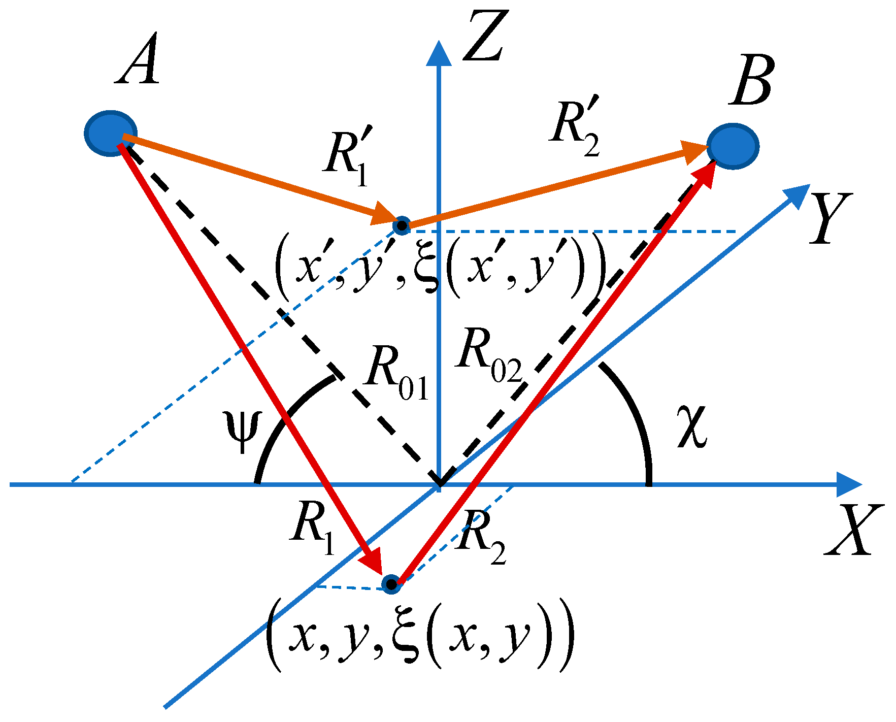
Consider the quasi-specular reflection of waves in the bistatic formulation of the problem in
Figure 1.
The undisturbed water surface coincides with the XY plane. The ordinates of a large-scale [
20,
21] water surface are described by the function
with a Gaussian wave height distribution. In contrast to the previous work [
19], here we consider a particular case of wave propagation along the
X or
Y axis. Suppose that A is the transmitting point and B is the receiving point. The transmitter simultaneously radiates spherical waves with a wavenumber
, and
, where
is the radiation wavelength. We will assume that the wave numbers differ slightly from each other:
The distance from the emitter to the current points and is equal to and , respectively. The distance from the current points and to the receiver is equal to and , respectively. The grazing angle of the transmitting antenna is , and that of the receiving antenna is .
We assume that the transmitter and receiver have common antennas for both frequencies. The receiver
and transmitter
antennas may differ. The antenna pattern is described by the Gaussian form:
where
and
are the distances from the center of the scattering area to the transmitter and receiver, respectively.
,
,
and
are the widths of the antenna patterns at the half power level for the emitting and receiving antennas in two planes, respectively.
With a small deviation of the receiver from the specular beam (<20–25°), it is possible to write an expression for the voltage at the output of the receiving antenna for each frequency using the Kirchhoff approximation:
where
is the scattering vector,
and
are the amplitudes of the emitted fields at two frequencies, and
is the effective reflection coefficient taking into account signal attenuation due to scattering on a small-scale surface.
We expand the distances to the current points in a Taylor series:
where
,
,
,
,
, and
for the given statement of the problem, and
and
are shifts in coordinates. Since these expansions will be used when calculating the correlation function of signals, these shifts are very small, within the surface correlation radius. Derivatives in this formula are expressed as follows:
2.2. Cross-Correlation Function
Next, we write the expression for the cross-correlation function of the received signals in the form:
Let us substitute here the expressions for the received signals (3):
When averaging the exponent with ranges, averaging occurs only over the surface ordinates:
where
,
,
, and
.
According to the definition of the characteristic function of a two-dimensional random variable, we write:
where
,
, and
are the sea surface statistical parameters.
Next, we move from the cross-correlation function to the correlation coefficient, having normalized to the intensity:
The experiment will measure the modulus of the correlation coefficient:
As a result of successive integration (6), normalization and calculation of the modulus, we obtain the following expression for the modulus of the cross-correlation coefficient, which will be referred to as the signal correlation coefficient (SCC):
where
,
,
, and
.
It can be seen from the obtained expression that the SCC depends on the distances from the center of the reflecting area to the transmitter and receiver, the wave height variance, the wave slope variance, the antenna patterns and the wavenumbers of the emitted signals. The SWH is calculated as four squared roots of the height variance.
3. Results
All dependences were calculated for electromagnetic radiation in the Ku-band. First, let us compare the dependences of the SCC on the SWH in the bistatic and monostatic sensing geometries in
Figure 2. The wave slope variances are the same in all cases and correspond to fully developed waves for a wind speed of 8 m/s [
22]. The beamwidths of all antennas are equal
. The distances from the center of the reflecting area to the transmitter and receiver are 10 km.
This is the main dependence of the approach used, showing the sensitivity of the SCC to the SWH for three variants of the frequency bases of the emitted waves. The maximum sensitivity (derivative) for different SWH is achieved at different . Thus, to ensure the high accuracy of SWH measurements, it is necessary to use several frequency bases.
It can be seen from the figure that in the bistatic problem statement, the SCC slightly increases, as well as when the axis of the receiving antenna deviates from the specular reflection beam. This is since the number of reflecting facets of the water surface decreases with a deviation from the specular reflection and the analyzed area on the water surface decreases and, accordingly, the correlation of the received reflected signals increases.
Let us compare the dependences of the SCC on the angle of deviation of the axis of the receiving antenna from specular reflection in the bistatic and monostatic cases in
Figure 3. For the monostatic case, this means the deviation of the axis of the transceiver antenna from the vertical. The grazing angle for vertical probing is 90 degrees. For the bistatic case, we fix the grazing angle of the axis of the transmitting antenna equal to 80 degrees and change the grazing angle of the receiving antenna. The distances from the center of the reflecting area to the transmitter and receiver are 10 km.
As in the previous figure, with an increase in the angle of deviation from the specular direction, the correlation of the two signals increases. Moreover, for the monostatic case, the correlation grows faster, since the reflecting area decreases faster, as both the receiving and emitting antennas simultaneously deviate. However, the power of the reflected signal in the monostatic case will also fall faster with the deviation angle from the vertical. To sum up, when the receiving antenna deviates from the direction of specular reflection, the correlation does not decrease; however, it must be remembered that the signal level decrease sharply (in the monostatic case by about 10–15 dB with a deviation of 10° from the vertical), which can reduce the accuracy of measuring the SCC value.
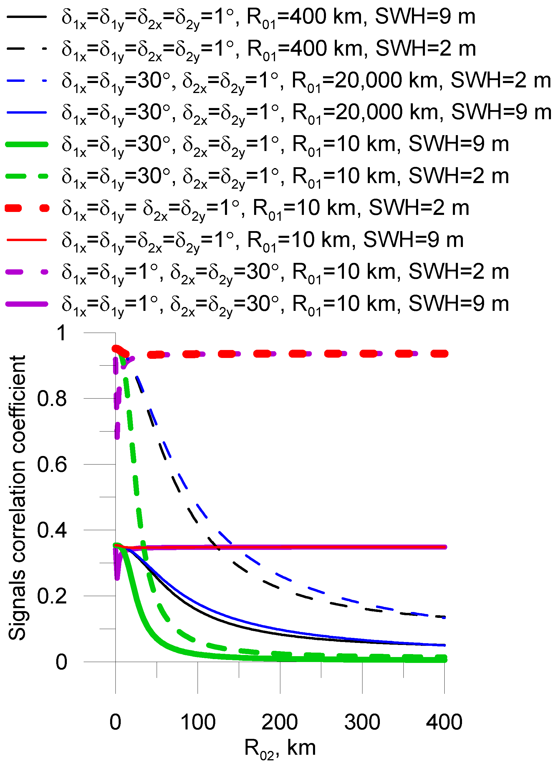
Let us construct the dependence of the SCC on the distance of the receiver at different distances from the transmitter (20,000 km, 400 km, and 10 km) in the case of using a wide and narrow antenna pattern of the transmitting and receiving antennas in
Figure 4. The grazing angle of the receiving and transmitting antennas is 80 degrees at a bistatic formulation of the problem. The frequency base
in all cases is 15 MHz.
Solid lines are always drawn for SWH = 9 m, and dotted lines are drawn for SWH = 2 m. The figure shows that even with a narrow antenna pattern of the transmitting and receiving antennas at a transmitter distance of 400 km (solid and dashed black lines), the SCC quickly decreases from the distance to the receiver and becomes so small at an altitude of 400 km that the dynamic range of the SCC values will not be enough to retrieve the SWH with high accuracy. That is why this SWH retrieval method is difficult to use in orbit. When increasing the altitude and width of the antenna pattern of the transmitter to the values corresponding to the navigation satellites (solid and dashed blue lines), this situation persists. In this case, the SWH retrieval method from the SCC will work only at short distances to the receiver. Lowering the transmitter with a wide antenna pattern to 10 km (solid and dashed green lines) further increases the limitation on the distance to the receiver. However, if the transmitter antenna pattern is narrow at a short distance (red for a narrow receiving antenna pattern and purple for a wide receiving antenna pattern, solid and dashed lines), then the SCC becomes insensitive to the distance to the receiver and the antenna pattern of the receiver. The insensitivity of the SCC to the receiver distance always occurs when the water surface area from which the reflected radiation is received exceeds the area of illumination by the transmitting antenna. A narrow transmitting antenna at a low altitude limits the area of illumination on the water surface and the spread of radiation propagation ranges will not depend on the distance to the receiver or receiving antenna. The measurement scheme where one of the antennas (transmitting or receiving) is at a low altitude allows us to fully use the different sensitivities of the SCC to the SWH at different frequency bases and provide high measurement accuracy over the entire range of SWH. This geometry appears most preferable in the practical implementation of this method: one antenna (transmitting or receiving) with a narrow antenna pattern is located at a low altitude, and another with a wide antenna pattern is located on a spacecraft.
Let us construct the SCC dependence on the frequency base
for different SWH in
Figure 5. The grazing angle of the receiving and transmitting antennas is 80 degrees in the bistatic formulation of the problem.
The figure shows that with an increase in the frequency base of the transmitted signals, the SCC always decreases. In addition, with an increase in the width of the antenna pattern of the receiving and transmitting antennas, and, consequently, with an increase in the “illuminated” area of the water surface, the difference between the SCC at high and low SWH decreases, i.e., SWH measurement will be worse. It can also be seen from the figure that for all cases, the largest difference in SCC for an SWH interval of 2–9 m will be maximum at a frequency base around 25 MHz, and therefore the accuracy of measuring the SWH will be higher. Next, we will check the influence of the slope variance on the SCC when using different antenna patterns of the receiving and transmitting antennas in
Figure 6.
The dependencies are constructed on the so-called total slope variance, which is the sum of the slope variances in two perpendicular directions and characterizes the overall roughness of the water surface. The grazing angle of the receiving and transmitting antennas is 80 degrees for the bistatic problem statement.
It can be seen from the figure that an increase in the slope variance leads to a decrease in the SCC. This is explained by the fact that a larger area of the water surface begins to be considered in the reflection. The figure also shows that if one of the antennas is narrow (1 degree), then the SCC will not be sensitive to slope variance.
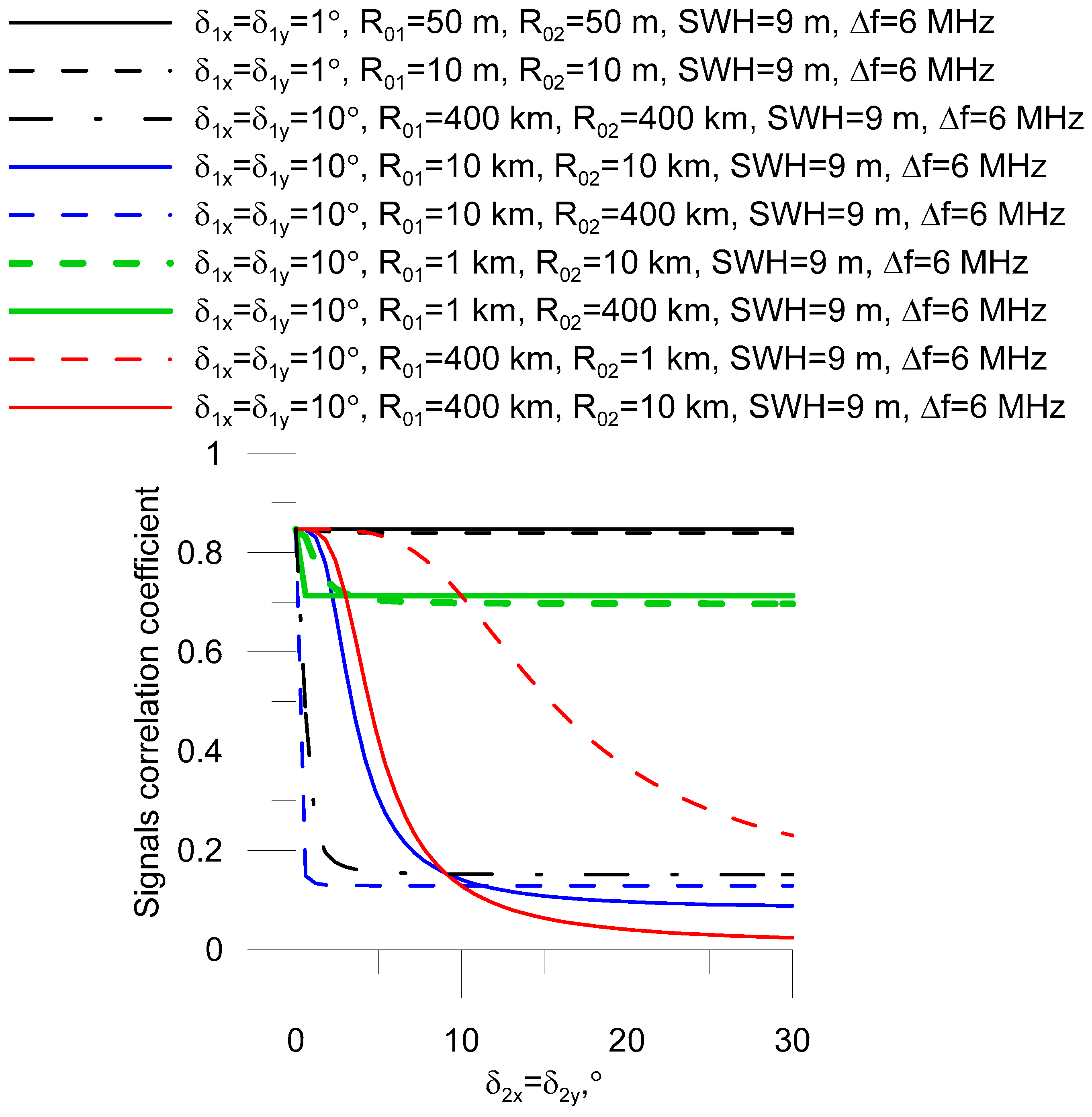
Consider the influence of the receiving and transmitting antenna patterns on the SCC in various measurement geometries in
Figure 7. We consider symmetrical antenna patterns
. The grazing angle of the receiving and transmitting antennas is 80 degrees for the bistatic formulation of the problem.
The figure shows that when using a narrow transmitting antenna at short distances to the transmitter, the receiving antenna does not affect the SCC. When using a wide transmitting antenna beamwidth, increasing the beamwidth of the receiving antenna will decrease the SCC until the area of the water surface involved in reflection stops increasing. Moreover, the effect on the SCC will be greater the farther the transmitter is from the center of the reflection area on the water surface. The SCC will decrease with the growth of the receiving antenna pattern faster the farther from the center of the reflection region the receiver is located.
4. Discussion
It can be concluded that the SCC is proportional to the spread of radiation propagation distances and is determined by the size of the reflecting area of the water surface. For better operation of the SWH measurement algorithm by the SCC, it is necessary to minimize the area of water surface illumination. However, also it is also important to not forget about the power of the reflected signal, because if there is no reflected signal, in theory it will give a high correlation, but in practice the signal will “drown” in noise. As a result, it is necessary to choose a geometry close to the geometry of receiving specularly reflected radiation and limit the reflecting area of the water surface by narrowing and lowering the transmitting or receiving antenna as much as possible. In this case, another antenna (receiving or transmitting) can be located at any height up to satellite.
The resulting expressions and dependencies allow us to choose the SWH measurement scheme in the bistatic problem statement. From the point of view of global coverage, the measurement scheme appears optimal, where one of the antennas (receiving or transmitting) is located on the satellite and the other is located on a beacon or aircraft.
The final formula also includes wave slope variances in two perpendicular planes, which opens the possibility of retrieving these parameters using antenna systems of several receiving antennas with different antenna patterns.
It is important that for underwater acoustic sounding all formulas remain operable. Accordingly, such a method for measuring SWH in sonar can be applied. Bistatic sonars can be installed, for example, in ports to monitor the area of the water surface remotely from the transmitter and receiver.
The next step in this research should be a bistatic experiment in which it is necessary to check the obtained dependencies.
Existing satellites cannot be used to test the proposed approach. The proposed approach requires a certain set of emitted frequencies providing a set of frequency bases and requires special processing of raw reflected signals.
Traditionally, before the launch of satellites, flight tests of new equipment are carried out. To develop the proposed approach, the first bistatic experiments should be carried out on the ground, installing the receiver and transmitter on two neighboring bridges across a river. In experiments, SWH must be controlled using a contact method, for example, with a string wave gauge. Measurements of the correlation coefficient of reflected signals must be carried out for several frequency bases of the emitted signals. It is necessary to compare the obtained experimental dependences of the bistatic correlation coefficient on SWH with the theoretical ones. Moreover, the experiments on the river are also justified by the fact that it will be possible to check the accuracy of the approach for small values of SWH, for which the traditional algorithm based on the analysis of the reflected pulse shape will not work. Then, it is worth moving on to flight tests, in which the receiver will be located on an aircraft, and the transmitter of two signals is close to the ground—for example, on a bridge. In an aircraft experiment, an important point will be the selection of diagrams of the transmitting and receiving antennas to track the moment when the correlation coefficient of the two reflected signals reaches a constant level with increasing flight altitude.
5. Conclusions
In this study, an explicit relationship was obtained between the SCC and the wave parameters. For the first time, the final expression is given for the bistatic problem statement. When deriving, three parameters of the reflecting surface are considered: SWH and slope variances in two perpendicular planes. In the formulas, it is possible to independently change the grazing angles of the receiving and transmitting antennas, the distance from the center of the reflecting area to the transmitter and receiver, as well as the width of the antenna patterns in two planes. The advantage of using the bistatic problem statement is the possibility of monitoring the area of the water surface at a large distance from the transmitter and receiver and, at the same time, remaining in the quasi-specular reflection region, which is well described by Kirchhoff’s approximation.
From the above expressions and figures, it follows that the cross-correlation function of two signals spaced in frequency in the bistatic formulation of the problem can be used to determine the SWH with high accuracy over the entire range of SWH. Moreover, the accuracy of the algorithm will be highest when placing a transmitter or receiver with a narrow symmetrical antenna pattern at an altitude of up to 10 km. In this case, another antenna (receiver or transmitter) can be located at any altitude up to being placed in Earth orbit without restrictions on the antenna pattern.


