Article

Optimal Estimation Inversion of Ionospheric Electron Density from GNSS-POD Limb Measurements: Part II-Validation and Comparison Using NmF2 and hmF2

by
Nimalan Swarnalingam
1,2,*,
Dong L. Wu
1,
Daniel J. Emmons
3 and
Robert Gardiner-Garden
4
1
NASA Goddard Space Flight Center, Greenbelt, MD 20771, USA
2
Department of Physics, The Catholic University of America, Washington, DC 20064, USA
3
The Air Force Institute of Technology, Wright-Patterson AFB, Dayton, OH 45433, USA
4
The University of Adelaide, Adelaide 5005, Australia
*
Author to whom correspondence should be addressed.
Remote Sens. 2023, 15(16), 4048; https://doi.org/10.3390/rs15164048
Submission received: 6 May 2023 / Revised: 20 July 2023 / Accepted: 25 July 2023 / Published: 16 August 2023

Abstract

:
A growing number of SmallSat/CubeSat constellations with high-rate (50–100 Hz) global navigation satellite system radio occultations (GNSS-RO) as well as low-rate (1 Hz) precise orbit determination (GNSS-POD) limb-viewing capabilities provide unprecedented spatial and temporal sampling rates for ionospheric studies. In the F-region electron density (N e ) retrieval process, instead of the conventional onion-peeling (OP) inversion, an optimal estimation (OE) inversion technique was recently developed using total electron content measurements acquired by GNSS-POD link. The new technique is applied to data acquired from the COSMIC-1, COSMIC-2, and Spire constellations. Although both OE and OP techniques use the Abel weighting function in N e inversion, OE significantly differs in its performance, especially in the lower F- and E-regions. In this work, we evaluate and compare newly derived data sets using F2 peak properties with other space-based and ground-based observations. We determine the F2 peak N e (NmF2) and its altitude (hmF2), and compare them with the OP-retrieved values. Good agreement is observed between the two techniques for both NmF2 and hmF2. In addition, we also utilize autoscaled F2 peak measurements from a number of worldwide Digisonde stations (∼30). The diurnal sensitivity and latitudinal variability of the F2 peak between the two techniques are carefully studied at these locations. Good agreement is observed between OE-retrieved NmF2 and Digisonde-measured NmF2. However, significant differences appear between OE-retrieved hmF2 and Digisonde-measured hmF2. During the daytime, Digisonde-measured hmF2 remains ∼25–45 km below the OE-retrieved hmF2, especially at mid and high latitudes. We also incorporate F-region N e measurements from two incoherent scatter radar observations at high latitudes, located in the North American (Millstone Hill) and European (EISCAT at Tromso) sectors. The radar measurements show good agreement with OE-retrieved values. Although there are several possible sources of error in the ionogram-derived N e profiles, our further analysis on F1 and F2 layers indicates that the low Digisonde hmF2 is caused by the autoscaled method, which tends to detect a height systematically below the F2 peak when the F1 layer is present.

1. Introduction

The F-region electron density (N e ), which can typically be found between 160 and 500 km, is mainly produced by extreme solar UV radiation and X-rays. While these sources are dependent on the solar zenith angle and its variation, soft particle precipitation from the magnetosphere and solar wind also produce a significant level of ionization at high latitudes under geomagnetically disturbed conditions. Being closely coupled to the neutral thermosphere and overlying magnetosphere, the F-region plasma behavior is mainly controlled by chemical processes at lower altitudes and diffusive and other transport processes at higher altitudes. During the daytime, the region generally splits into two regions, with the lower region being the F1 layer (peaks at ∼160–200 km) and the higher region being the F2 layer (peaks at ∼300–350 km). The two regions merge into one during nighttime. The F2 layer, which has the greatest concentration of N e , is the most variable and the most anomalous region. Variation in chemical composition, especially in atomic oxygen and molecular nitrogen, and their temperature sensitivity can cause changes in N e , which are, in turn, transported by electric fields and neutral winds. For example, in the equatorial region, equatorial ionization anomaly (EIA) is created during the daytime by upward E × B drift, and causes crests with an accumulation of N e within ∼±20 geomagnetic latitudes (e.g., [1]). These features are enhanced during geomagnetically disturbed conditions, leading to variations in both the F2 peak N e (NmF2) and its altitude (hmF2).
For several decades, ionospheric N e measurements have been mainly made using ground-based radio wave techniques such as ionospheric sounding (ionosonde) and incoherent radar scattering, as well as occasional space-borne topside sounders. Vertical incidence ionospheric sounders transmit a sweep of frequencies in the high-frequency (HF) band (∼1–30 MHz), and the time delay of the reflected signals are measured [2]. As the wave penetrates further into the ionosphere, the energy is reflected at the level where the plasma frequency is equal to the probing wave frequency (i.e., critical frequency). Hence, the travel time of the pulses at different frequencies allows to associate a reflecting height for a given frequency on a graphical plot, an ionogram [3]. Since the transmitted signals travel slower in the ionosphere than in free space, the observed altitudes are called virtual heights, which exceed the true reflection heights. Subsequently, an inversion algorithm is used to retrieve the true heights of the reflected signals, and hence, N e as a function of altitude [2]. In ionosondes, since the measurements can only be made up to the F2 peak altitude, modeled true heights are used above the F2 peak. Over the years, extensive developments have been made in the sounding technique, especially in measuring the time of flight, polarization, absorption due to collision, and Doppler shift of signals as a function of frequency (e.g., [4,5,6]). Modern digital ionosondes can automatically calculate N e profiles in near real time using automated software systems [7], and subsequently, data are sent to a central repository system [8].
In the case of incoherent scatter radar (ISR), scattering arises due to thermal fluctuations in electron density, known as Thomson scatter [9]. The technique is one of the most powerful and flexible tools to observe and continuously monitor the ionosphere. Unlike ionosondes, the frequency of incoherent scatter radar is much higher than the plasma frequency in the ionosphere to ensure that the waves pass through the plasma without perturbing. Hence, it can receive echoes from spatial density fluctuations, both the top and bottom sides of the F2 peak. The scatter is indeed from the spatial component in the spectrum of the ion-acoustic and electron-acoustic waves in the ionospheric plasma [10]. Scattering occurs when the Bragg scatter condition is matched, in which the spatial scales are half the wavelength of the probing radar. Although both ionosondes and ISRs make reliable routine measurements, they are limited in number, and make single-location observations only over inland areas, leaving no coverage in ocean areas.
In recent decades, sounding techniques using the radio-link between SmallSat/CubeSat constellations and global navigation satellite systems (GNSSs) have become one of the major techniques for global atmospheric and ionospheric observations [11]. Although in the early years, high-rate radio links (50–100 Hz) from radio occultation (RO) antennas were mainly utilized for measurements, low-rate radio links (1 Hz) from precise orbit determination (POD) receiver antennas have also been greatly utilized in recent years (e.g., [12,13]). In the case of F-region N e retrieval, the onion-peeling (OP) inversion technique has been conventionally used over the years [14]. The retrieved N e profile is based on Abel inversion, which requires a spherical symmetry assumption. Studies have shown that this could cause errors at lower altitudes (∼below 200 km), where in general, the horizontal gradients in N e are relatively large and prominent [15,16]. In recent years, improvements in the OP inversion technique (e.g., [17,18,19]), as well as alternative approaches [20], have been proposed to improve the accuracy of N e retrieval. The improved versions of OP retrieval have been utilized in several ionospheric studies and have become a useful tool to explore large-scale Ne studies, especially in the F-region (e.g., [21,22]). Recently, an optimal estimation (OE) inversion technique was developed using total electron content measurements acquired by the GNSS-POD link [23]. Although the OE inversion algorithm also uses the same input parameters as in the case of OP inversion, the former shows some unique features, and in particular, its results significantly differ in the lower ionosphere, as will be described shortly.
In this work, we provide an evaluation of the OE inversion technique along with its capabilities in a wide variety of ionospheric studies. The technique is applied to all GNSS-POD data acquired from the COSMIC-1, COSMIC-2, and Spire constellations. We determine NmF2 and hmF2 in OE-retrieved N e profiles and perform climatological comparisons with preexisting OP-retrieved data. In addition, we also use NmF2 and hmF2 measurements from a number of worldwide Digisonde locations along with two ISR observations, located in the North American (Millstone Hill) and European (EISCAT at Tromso) sectors. Following the description of the different types of data sets, the application of our strict quality control procedures, as well as the determination of NmF2 and hmF2 values, are described in Section 2. The estimated NmF2 and hmF2 values from the two different inversion techniques are compared in Section 3.1. Subsequently, in Section 3.2, NmF2 and hmF2 measurements from ∼30 global Digisonde stations are used to compare and analyze diurnal sensitivity and latitudinal variability among these data sets. The OE-retrieved N e profiles are compared to ISR measurements in Section 3.3, followed by discussion and conclusions.
In the Discussion section, we present an extensive discussion in Section 4.1 related to the observed differences between the OE-retrieved and Digisonde-measured hmF2 values, especially during the daytime. We also discuss the possible reasons for this disagreement between them in Section 4.1.1. In addition, we also describe some of the other capabilities in Section 4.2, in particular investigating the topside and bottomside of the F2 layer in relation to the shape of the N e profile.

2. Materials and Methods

2.1. Space-Borne Data Sets

The newly developed OE inversion technique, namely OE/v6p, utilizes GNSS-POD limb sounding total electron content (hTEC) measurements. The hTEC profile is a function of tangent height, defined as an integrated TEC along the limb where the elevation angle is negative [20]. Thus, the retrieved N e from GNSS-POD is only valid at altitudes below the orbital height of the satellite. A detailed description of the OE inversion technique can be found in [23]. The technique is applied to three SmallSat constellations: COSMIC-1, COSMIC-2, and Spire, and the derived F-region N e data sets from COSMIC-1 and COSMIC-2 are compared and evaluated using preexisting N e retrievals, in which the conventional OP inversion technique was applied. The latter data set was obtained through the COSMIC Data Analysis and Archive Center (CDAAC). As in the case of the OP technique, the OE technique also uses the Abel weighting function in the N e inversion. However, it significantly differs in its performance in the lower ionosphere; in particular, the new OE results can overcome the large N e oscillations, sometimes negative values, seen in the OP retrievals in the lower F- and E-region ionosphere. Figure 1 shows an example of OE (red) and OP (black) retrieved N e profiles at two geographical locations using measurements from COSMIC-1 (left) and COSMIC-2 (right). In the figure, the OE- and OP-retrieved N e profiles, which are from the measurements taken within a short time interval, show disagreements, especially at low altitudes. The left side of the figure shows an example in which the OP-retrieved N e profile monotonically increases with decreasing altitude, whereas the right side shows an example for negative N e values starting at ∼250 km and below.
To further analyze the differences between these two techniques, we utilize globally available OE- and OP-retrieved profiles from COSMIC-2 observations during 1–10 December 2021 and establish distributions of N e values for lower altitudes during local 11–13 hours. Table 1 summarizes their means and standard deviations from 150 km down to 90 km, along with number of samples (shown in brackets). As is noticeable in the table, although the OP-retrieved mean and standard deviation agree reasonably well with OE retrieval at 150 km, they start to deviate from OE values at lower altitudes. At 90 km, the mean N e for the OP retrieval becomes negative with a high standard deviation, confirming the oscillatory and negative nature of the OP-retrieved profiles. Furthermore, the number of samples that are available in OP retrieval is significantly lower than OE retrieval, and it further decreases at 90 km. This indicates that some of the OP-retrieved N e profiles do not reach down to low altitudes. Nonetheless, as we will see shortly, these observations in the OP retrieval will not impact our current study, since both profiles reasonably agree well in the F-region.
In our analysis, we determine NmF2 and hmF2 values and compare them globally for given temporal and spatial intervals. To ensure accuracy and consistency, we apply a strict quality control check procedure on both data sets, as described below.
1.
We determine the initial NmF2 and hmF2 values for retrieved profiles within an altitude range. Although F2 peak altitudes tend to stay generally below 400 km, previous studies indicate occasionally higher values, especially at equatorial latitudes [24,25]. Hence, we set this range as 150–500 km. In some cases, the profiles are modulated with saw-tooth-like perturbation. Figure 2 shows such an example for the OE-retrieved N e profile from the Spire constellation during June 2021. We apply a 7-point sliding window filter to smooth all profiles (shown in red), and re-evaluate NmF2 and hmF2 values to ensure that the initial and final values of hmF2 are not exceeded by 10 km.
2.
In the OE inversion algorithm, the input parameter hTECs are fed only when their measurements are present for all tangent heights from the satellite orbital altitudes (∼450–600 km) down to ∼100 km. However, as shown above, such strict criteria are not generally applied in the case of OP inversion, and hence, large spatial gaps are present in some of the OP-retrieved N e profiles. To ensure that our data sets are not affected by this, we check the continuity of these profiles within the selected altitude range. If any missing data are evident for more than a 10 km altitude range, the respective profile is discarded from the analysis. To further strengthen our selection criteria, we also discard any monotonically increasing or decreasing N e profile, i.e., if the detected hmF2 occurs within 10 km of the lowest or highest edge of the set altitude range (150–500 km), the profile is discarded.
3.
The estimated NmF2 and hmF2 values are then binned into a 5 latitude by 10 longitude grid for each hour. To perform a comparison study with Digisondes and radars with meaningful statistics, we need to maintain the above grid size for OE-retrieved measurements. In addition, we also identify the thickness of the retrieved F2 layer with 95%, 90%, and 80% of NmF2. The estimated F2 layer thicknesses from the OE retrieval are later used for comparison with Digisonde measurements.

2.2. Ground-Based Data Sets

2.2.1. Digisondes

We compare and evaluate the OE-retrieved NmF2 and hmF2 values with a number of global Digisonde measurements. Figure 3 shows 30 Digisonde stations along with their respective locations used in this study. The map also contains lines of constant geomagnetic latitude based on apex geomagnetic coordinates referenced to an altitude of 350 km [26]. The geomagnetic equator is shown by a dashed line, and ±10 geomagnetic latitudes are shown by dotted lines. Most of the global locations are now operated by Digisonde Portable Sounders (DPS version 4D), which are capable of making measurements of the overhead ionosphere and providing real-time on-site automatic scaling, namely the Automated Real-Time Ionogram Scaler with True height (ARTIST) software (Version-5) [7]. Subsequently, data are sent to the Digital Ionogram DataBase (DIDBase) repository [8]. The data used in this study were gathered from the Global Ionosphere Radio Observatory (GIRO).
While automatically scaled ionograms are prone to errors and uncertainty [27,28,29], manual scaling is unfeasible for large data sets such as those used in this study. Additionally, a recent study found that ARTIST F2 peak frequency (foF2) estimations agree with manually scaled values for ∼95% of ionograms [30]. Therefore, we believe that our decision to compare the OE-retrieved NmF2 and hmF2 values strictly to Digisonde measurements autoscaled with ARTIST-5 is justified for this large data set. Systematic biases between the OE retrieval results and the autoscaled ionograms can help to guide future improvements and refinements for one or both techniques. In the Digisonde ionogram autoscaling procedure, ARTIST-5 maintains a measure of quality assurance by providing confidence scores (CS) [31]. The CS score starts with a value of 100 (maximum) and decreases when encountering uncertainties or unusual profiles. Although the acceptable value of CS is above 40, in our case, we use data with CS higher than 80 to reduce uncertainty.

2.2.2. Incoherent Scatter Radar

In addition to Digisondes, we also use measurements from two ISRs located at Millstone Hill (42°N, 72°W) and Tromso (70°N, 19°E). As described in Section 1, unlike Digisonde, the frequency of the ISR is much higher than the plasma frequency in the ionosphere; thus, the waves pass through the plasma. Hence, ISRs make measurements for the entire ionosphere typically from ∼90 km, with a time resolution on the order of minutes. This allows to compare not only the OE-retrieved NmF2 and hmF2 values, but also the entire N e profiles with ISR measurements. It is generally considered that ISRs provide the most accurate measurements of N e . However, their ability to provide a global morphology is limited, since they are limited in number due to high installation and maintenance costs. The radar data used in this study were gathered from the Coupling, Energetics, and Dynamics of Atmospheric Regions (CEDAR) Madrigal Database.

3. Results

We consider selected months for 2008, 2011, 2012, 2021, and 2022 to compare the OE-retrieved NmF2 and hmF2 values with the OP-retrieved NmF2 and hmF2 values, as well as with ∼30 Digisondes and two radar measurements. Selection of the months and years are based on the optimal availability of all data sets relevant to this study.

3.1. Climatological Comparison of Global NmF2 and hmF2 Maps

In this section, we compare the estimated NmF2 and hmF2 values from the OE and OP inversion techniques. We produce global maps of NmF2 and hmF2 from the retrieved N e profiles for COSMIC-1 and COSMIC-2 constellations. Applying the OE inversion technique on COSMIC-1 measurements produces ∼700–1600 N e profiles per day for the period of the investigation (June 2008). Among those, ∼5–7% are discarded due to the application of our strict quality control procedure. In the case of OP-retrieved N e profiles, ∼1000–2000 profiles are available. However, ∼17–22% fails to pass our quality control measure. As described in Section 2.1, the occasional existence of data gaps larger than 10 km of altitude in the OP-retrieved N e profiles is the main cause for this difference to occur. From retrieved N e profiles, we establish monthly global NmF2 and hmF2 maps. To ensure consistency, we establish 5 latitude by 10 longitude bin size maps for both retrieval techniques. Figure 4 shows a comparison of NmF2 from OE and OP techniques applied to COSMIC-1 measurements during June 2008. The figure compares the two retrievals at selected 4-hour universal time (UT) windows. The left column shows a global map of NmF2 from OE-retrieved profiles for 00–04 UT, 10–14 UT, and 16–20 UT. The middle column shows the same for OP retrieval. The right column shows scatter plots between the two retrieved NmF2 values for respective universal time intervals, in which local midday (10–14 LT) and midnight (22–02 LT) hours are marked by red and blue, respectively. The figure shows good agreement between the two techniques. It is also noticeable in scatter plots that NmF2 values from OE and OP techniques agree well both during local midday (red) and midnight (blue) hours, especially for low and moderate NmF2 values. However, a slight increase in standard deviation is also evident at high NmF2 values.
In COSMIC-2, a high sampling rate produces ∼6000 N e or more profiles per day (since 2021). However, it has limited coverage only within ±45 latitudes. Figure 5 shows the same comparison using the measurements from COSMIC-2 during June 2021. As in the case of COSMIC-1, good agreement between the two techniques is evident in COSMIC-2 as well. The data shown for COSMIC-1 and COSMIC-2 are from solar minimum years of cycles 23/24 and 24/25. Although it is generally expected that NmF2 values may smear out, especially in the EIA region due to strong horizontal gradients, such impacts are not prominent in either COSMIC-1 or COSMIC-2 results. These results are in agreement with previous NmF2 studies using COSMIC-1 [32] and COSMIC-2 [21], implying that the impact due to the assumption of ionospheric spherical asymmetry may not influence the F2 peak measurements.
Figure 6 and Figure 7 show a comparison of hmF2 between the two techniques for the data collected during June 2008 and June 2021 by COSMIC-1 and COSMIC-2, respectively. Overall, good agreement is present between the OE- and OP-retrieved hmF2 estimations. However, differences appear in scatter plots (right column), especially during local midday hours (red) for low altitudes. Note that we applied the same OE retrieval algorithm in both constellations. The COSMIC-2 has geographical coverage only within ∼±45 latitudes, whereas COSMIC-1 has coverage for ∼±85 latitudes. Nevertheless, COSMIC-2 has a better sampling rate compared to COSMIC-1. It is noticeable in figures that the degree of agreement between the OE- and OP- hmF2 values improved from COSMIC-1 to COSMIC-2.
The OE inversion retrieval technique is also successfully applied to Spire constellation [23]. Figure 8 shows global maps of NmF2 and hmF2, estimated during local 10–14 hours in June 2021. The Spire constellation has global geographical coverage, along with a reasonably good sampling rate [23]. This is evident in Figure 8, as it contains a minimal number of gaps compared to COSMIC-1 (Figure 4 and Figure 6).
As expected, Figure 8 shows higher NmF2 values along the EIA region (upper panel). The equatorward neutral winds tend to move F2 region plasma to a higher altitude in the EIA region, where the recombination rate is relatively low, leading to enhancements in the EIA crests (e.g., [1]). Studies have also shown that winds often cause net transport of plasma from the summer to winter hemisphere, leading to asymmetry in the formation of EIA crests, which are, in turn, modulated by tides, resulting in longitudinal variability [33]. On the other hand, relatively higher hmF2 values are present on the northern side of the EIA crest region (lower panel). These results are also evident in COSMIC-1 and COSMIC-2, and moreover, these results show good agreement with previous studies [34]. The observed elevated hmF2 values in the southern EIA crest region could also influence the scale height above the F2 peak, and we will discuss this further in Section 4.

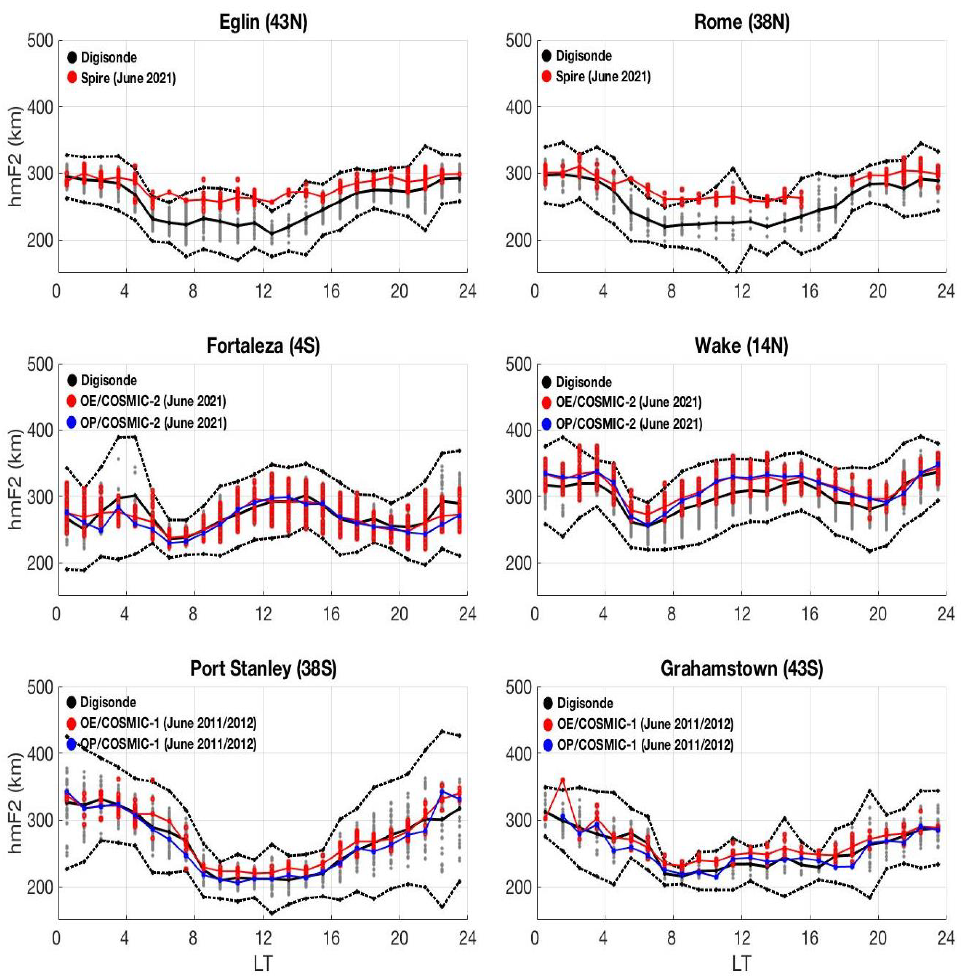
3.2. Comparison of OE-Retrieved F2 Peak Properties to Digisonde Measurements

Digisondes generally make measurements every 5–15 min. However, in this analysis, we use hourly means of NmF2 and hmF2 to match the sampling rates of the satellites. Additionally, since Digisondes are operated continuously during day and night, we can also perform a comparative diurnal sensitivity analysis between the two data sets, utilizing Digisonde measurements of NmF2 and hmF2. Figure 9 shows latitudinal variation of the hourly NmF2 means from OE retrieval (red) and Digisonde measurements (green), plotted in geomagnetic coordinates. The left column shows the measurements from COSMIC-1 during June 2011/2012. The middle and right columns show the measurements from COSMIC-2 and Spire, respectively, during June 2021. The top row compares the OE-retrieved NmF2 to Digisonde measurements for the full local day, and the middle and bottom rows compare for local midday hours (10–14 LT), as well as local midnight hours (22–02 LT). Generally, the figure shows good agreement between OE-retrieved and Digisonde NmF2 values for all three satellites. Better agreements are evident in the figure between COSMIC-2 (middle column) and Spire (right column), since both are from the same month/year period. However, they differ from COSMIC-1, which are from June 2011/2012. Note that 2011/2012 were in the rising phase of the solar cycle 24, while 2021 was a solar minimum year of cycle 25. As expected, NmF2 for June 2012 (left column) is higher by a factor of ∼2 compared to June 2021, especially during midday hours (middle and right columns). The COSMIC-2/Digisonde comparison (middle column) also consists of standard deviation values. Daytime standard deviations seem higher than nighttime values. While the standard deviations for the Spire/Digisonde comparison are very similar to COSMIC-2/Digisonde, the COSMIC-1/Digisonde values are higher by a factor of ∼2 (not shown due to the high density of data points).
Figure 10 shows a similar comparison for hmF2 between OE retrieval and Digisonde. The left column shows comparisons between COSMIC-1 and Digisonde at different local time windows for June 2012, whereas the middle and right columns show the same for COSMIC-2 and Spire, respectively, for June 2021. Significant differences appear between OE-retrieved hmF2 and Digisonde hmF2, especially during midday hours (middle row). Moreover, the differences seem higher in mid and high latitudes compared to the equatorial region. While Digisonde-measured hmF2 values are ∼5–25 km lower than the OE-retrieved values in the equatorial region, the differences between them increase to ∼25–45 km in mid and high latitudes. As in the case of the NmF2 comparison, the standard deviations for hmF2 estimates are shown only for the COSMIC-2/Digisonde comparison (middle column). While the standard deviations for the Spire/Digisonde comparison are very similar, the COSMIC-1/Digisonde values are relatively high by a factor of ∼2.
Following the comparison of latitudinal variation between OE retrieval and Digisonde measurements in Figure 9 and Figure 10, Figure 11 shows scatter plots of NmF2 and hmF2 between the OE retrieval and global Digisonde measurements. The upper row shows NmF2 and the lower row shows hmF2. In the figure, local time intervals of 0–24 LT hours, 22–02 LT hours, and 10–14 LT hours are marked by blue, cyan, and red dots, respectively. The figure reconfirms good agreement between OE-retrieved and Digisonde-measured NmF2, especially for COSMIC-2 and Spire. In the case of the hmF2 comparison, while COSMIC-2 and Spire show deviations from the Digisonde measurements (for June 2021), COSMIC-1 shows relatively better agreement with Digisonde measurements (for June 2011/2012). The reason for this could be associated with the fact that 2011/2012 were in the rising phase of the solar cycle 24 and closer to the maximum. It seems that the Digisonde-measured hmF2 values agree relatively better with OE- and OP-retrieved hmF2 during these times when NmF2 values are high, as we will discuss further in Section 4. However, in most cases, individual inspection at each Digisonde location shows evidence for consistent patterns of disagreements in both OE- and OP-retrieved hmF2 values with Digisonde-measured hmF2.
We further investigate the diurnal sensitivity of NmF2 and hmF2 between OE retrieval and Digisonde measurements. Figure 12 shows an example of NmF2 diurnal sensitivities among different data sets at six selected Digisonde stations. The top row has two stations (Eglin and Rome) that have similar geomagnetic latitudes in the Northern Hemisphere but at different longitudes, located in the American and European sectors, respectively. The middle row represents two stations (Fortaleza and Wake) at low geomagnetic latitudes, located in the American and Asian sectors. The bottom row includes two stations (Port Stanley and Grahamstown) in the Southern Hemisphere, located in the South American and African sectors, respectively. The top row compares OE retrieval from Spire to Digisondes for the data collected during June 2021. The middle and bottom rows compare OE retrievals from COSMIC-2 and COSMIC-1 to Digisonde measurements for the data collected during June 2021 and June 2011/2012, respectively. The OE-retrieved hourly values are shown as red dots, and the Digisonde hourly values are shown as green dots. The mean values are marked by solid lines with respective colors. Green dotted lines refer to the 3 σ boundary for Digisonde measurements (3 times the standard deviation). For completeness, we also include OP-retrieved NmF2 values (blue line) for COSMIC-1 and COSMIC-2 in the figure. As noted in Section 3.1, OP-retrieved data are not available for Spire when performing this analysis. It is noticeable that hourly mean NmF2 values from the three data sets (solid lines) show good agreement in general. Although the number of samples for these sites varies from site to site, they remain higher than 100. In the case of OE-retrieved hourly data, Grahamstown has the lowest number (108 samples during June 2011/2012), and Fortaleza has the highest (572 samples during June 2021). Digisonde sites have a relatively higher number of samples in general: Grahamstown has the lowest (180 samples during June 2012), and Port Stanley has the highest (643 samples during June 2012).
An example of a similar comparison but for hmF2 diurnal sensitivity for the same locations is shown in Figure 13. The OE-retrieved hourly hmF2 values are shown in red dots, and Digisonde hourly values are shown in gray dots. The mean values of OE retrieval and Digisonde measurements are shown by red and black solid lines, respectively. The 3 σ boundary for Digisonde measurements is shown by black dotted lines. The OP-retrieved hmF2 values are shown by blue lines. It is noticeable in the figure that while agreement exists among all three measurements during local midnight hours, differences appear during daytime. The daytime differences between the two techniques are very similar at Eglin and Rome (top panel), and also at Port Stanley and Grahamstown (bottom panel). This indicates that the differences between the Digisonde-measured and OE-retrieved hmF2 values are consistent and systematic along geomagnetic longitudes, at least in mid latitudes. We will notice similar trends at high latitudes as well when we incorporate ISR N e measurements in the following section.

3.3. Comparison of OE-Retrieved hmF2 with Incoherent Scatter Radar Measurements

While the OE-retrieved NmF2 values show good agreement with the Digisonde measurements, the estimated hmF2 values from OE retrieval show disagreement with the Digisonde measurements, especially during the daytime. To investigate this further, we use N e observations from two incoherent radar systems located at Millstone Hill and Tromso. Our comparison shows that OE retrievals reasonably agree with radar measurements. Figure 14 (left) shows an example of the OE-retrieved F-region N e profile at 10:16 UT (red) along with radar measured profiles at Millstone Hill during the 10 UT hour (blue dots) on March 16, 2007. For comparison purposes, we have also included the OP-retrieved N e profile (green). In particular, the hmF2 values of OE- and OP-retrieved profiles agree with the radar measurements. However, slight differences appear in the case of NmF2 values. Figure 14 (left) also contains an example of an OE-retrieved N e profile (dashed black) in which the calibrated hTEC values of CDAAC were used. Significant differences occur between green and dashed black profiles, especially in the vicinity of ∼10 km below the satellite orbital altitude. As already discussed in [23], the OE inversion technique uses an empirical calibration method, and ∼10 TECu offset in hTEC is evident between empirical calibration and the CDAAC’s hTEC calibration values, especially at satellite orbital altitudes (see Figure 4 in [23]). Nevertheless, as shown in Figure 14 (left), the N e values in the actual OP-retrieved N e profiles (green) obtained from CDAAC show good agreement with the OE-retrieved profile (red), especially closer to the satellite orbital altitude. The exact reason for this difference between the two N e profiles (green and dashed black) is not known, since detailed information related to CDAAC’s hTEC calibration values and their applications in the N e profiles, especially around satellite orbital altitudes, are not yet available in the literature to the best of our knowledge.
Figure 14 (right) shows a comparison of radar-measured hmF2 diurnal sensitivity with OE retrievals and Digisonde measurements. The upper panel refers to hmF2 measurements at Millstone Hill during June 2012. The hourly mean of the radar measurements is shown in blue along with OE retrieval from COSMIC-1 (red), as well as Digisonde measurements (gray and black). The lower panel refers to the measurements at Tromso during March 2022, in which OE retrieval from Spire is used. The comparisons at these two radar locations show that OE-retrieved hmF2 values agree better with radar measurements, especially during the daytime. However, differences are present, especially in midnight hours, and this is obvious at Tromso. Note that the Tromso site constantly stays under the auroral oval, and frequent precipitation events are common at this location. It can also be noticed in the figure that the standard deviations for the hourly Digisonde measurements are high during the night.
Finally, we also compare the climatological morphology of the F-region N e between OE retrieval and radar measurements. Figure 15 shows the contour plots of N e at Millstone Hill using OE retrieval from COSMIC-1 and ISR measurements during June 2012. A good agreement is evident between the two data sets, except for 5–10 LT, where slight differences appear.

4. Discussion

In the previous section, we compared OE-retrieved NmF2 and hmF2 with OP retrieval and Digisonde measurements. The OE-retrieved NmF2 values from COSMIC-1 and COSMIC-2 show good agreement with the OP-retrieved values (Figure 4 and Figure 5). In the case of hmF2, a slight deviation appears for midday hours, as is noticeable in the respective scatter plots (Figure 6 and Figure 7, right columns). It is also noticeable in those figures that the degree of agreement between the OE- and OP- hmF2 values improved from COSMIC-1 to COSMIC-2. Note that we applied the same OE retrieval algorithm in both constellations. Nevertheless, COSMIC-2 has a better sampling rate than COSMIC-1. Moreover, COSMIC-2 has coverage only within ±45 latitudes, whereas COSMIC-1 has coverage for ∼±85 latitudes. Therefore, it is possible that the differences occur due to the above reasons.

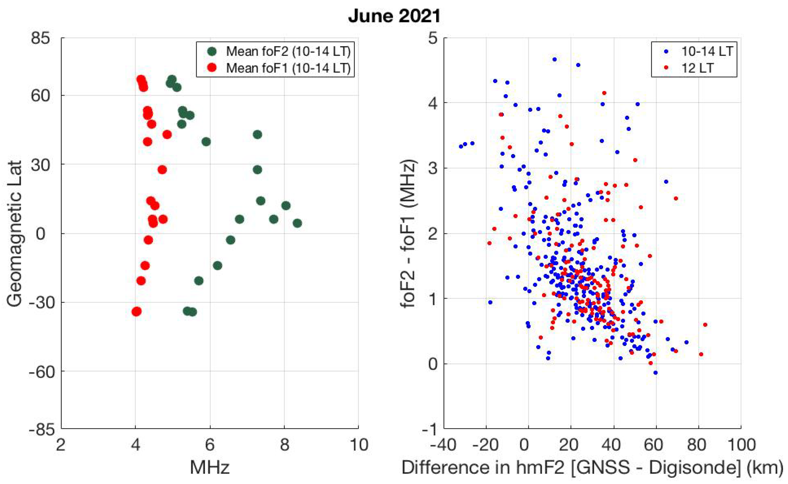
4.1. Differences in OE-Retrieved and Digisonde-Measured hmF2s

In the comparison of OE retrieval with Digisonde measurements, good agreement is present for NmF2. However, significant differences appear in the case of hmF2 during local daytime, as is evident in latitudinal variation analysis (Figure 10), as well as diurnal sensitivity analysis (Figure 13). This difference seems high at mid and high latitudes where the measured hmF2 values in Digisonde are on average ∼25–45 km below the OE-retrieved hmF2. Note that our Digisonde-measured F2 peak parameters are autoscaled values. While Digisonde-autoscaled NmF2 measurements agree well with OE-retrieved values (see Figure 11 upper row), the same software-autoscaled hmF2 values do not agree well, especially during local midday hours (Figure 11 bottom row). Hence, questions arise as to whether the Digisonde autoscaling procedure plays any role in the disagreement.
To verify this, we estimate F2 layer thicknesses using OE-retrieved N e profiles at 95% of NmF2 above and below the mean values of hmF2 and compare them with Digisonde hmF2 values. As an example, Figure 16 shows OE-retrieved F2 layer thicknesses at three locations: Chilton (top panel), Fortaleza (middle panel), and Hermanus (bottom panel) from COSMIC-1 and COSMIC-2. Chilton and Hermanus are located at mid latitude, whereas Fortaleza is located in the equatorial region. In this figure, the F2 layer thickness (dashed line) is considered at 95% of NmF2 above and below the mean values of hmF2 (solid red), and is plotted with Digisonde hmF2 measurements (black). It is noticeable that at Chilton (top panel) and Hermanus (bottom panel), Digisonde-measured hmF2 values remain at ∼95% of NmF2 or below, especially during the daytime. On the other hand, Digisonde hmF2 agrees with OE-retrieved hmF2 at Fortaleza.
Note that in our analysis, we use ARTIST-autoscaled F2 peak parameters with CS > 80. In contrast, manually scaled values (either fully or partially) were used in most of the previous studies (e.g., [21,35,36]). In a recent study on ARTIST CS numbers, it was found that the autoscaling procedure can detect the F2 layer almost 90% of the time when CS ≥ 40 [37]. This indicates that the CS numbers indeed act as a reasonable filtering parameter for the Digisonde F2 peak measurements. However, the main question here is whether the level of accuracy also increases along with higher CS numbers, particularly when interpreting virtual height measurements to the true heights.

4.1.1. Does the F1 Valley Cause Underestimations in Digisonde Autoscaled hmF2?

Although improvements have been made over the years in Digisonde-autoscaled procedures, recent evaluations among different autoscaling software indicate that differences still appear, especially with the accuracy of hmF2 [38,39]. In addition, it was also noticed in previous studies that the accuracy of autoscaling depends on local time, season, and solar activity (e.g., [40]). There are several possible sources of error in ionogram-derived N e profiles, including the “valley problem”, which describes the unknown width and depth of the valley between the E-region peak and the base of the F-region (see discussion in [41]). This valley problem is severe for lower magnitudes of the F2 peak critical frequency (foF2) because the inversion relies more heavily on modeled valleys. Additionally, ionograms with relatively small differences between foF2 and foF1 (F1 peak critical frequency) are dependent on estimated F1-region profiles that are often difficult to characterize [30,42,43]. Hence, hmF2 estimates from daytime ionograms with the F1-region present will possess larger uncertainties/errors for lower foF2 values. As an example in our case, Figure 17 shows Digisonde-measured foF2 (green) and foF1 (red) values for the Digisonde stations shown in Figure 16. It is noticeable that the separation between foF2 and foF1 is wider in the case of Fortaleza (middle panel) compared to Chilton (top panel) and Hermanus (bottom panel).
To investigate this with meaningful statistics, we consider Digisonde locations where autoscaled foF1 measurements are available and compare the differences of (foF2–foF1) with OE-retrieved and Digisonde-measured hmF2 values. Figure 18 (left) shows latitudinal variation of mean foF2 (green) and mean foF1 (red) at these locations during local 10–14 hours in June 2021. As is noticeable in the figure, the separation between foF2 and foF1 is larger at the equator and low latitude region, and it starts to decrease from the equator/low latitudes to mid and high latitudes. The latitudinal variation of (foF2–foF1) appears to be opposite to the differences in hmF2 observed between OE retrievals and Digisonde measurements (Figure 10 middle row). Figure 18 (right) shows the correlation between hourly (foF2–foF1) values and the differences in OE-retrieved and Digisonde-measured hmF2 values during local noon hours (red) and 10–14 hours (blue). As is evident in this figure, the separation between foF2 and foF1 maintains an inverse relationship with the differences in OE-retrieved and Digisonde hmF2 values in most cases. Although Spire OE-retrieved hmF2 values were used in the above case, verification with COSMIC-1 and COSMIC-2 also indicate a very similar relationship between (foF2–foF1) and the differences between OE-retrieved and Digisonde hmF2 values.
Hence, the error dependence on both foF1 and foF2 could explain our latitudinal trends in hmF2 differences where the GNSS retrievals and ionosonde estimations agree near the geomagnetic equator and differ at mid and high latitudes. Note that our results are based on an hourly climatology comparison. Our results are in agreement with the observations in previous studies and also with the recent error estimations in F2 layer peak parameters, especially for hmF2 using ARTIST-5 [39,40]. As pointed out in Section 2.1, to increase the number of data points in the OE retrieval, we had to consider a 5 latitude by 10 longitude region at each Digisonde location. While it is true that the F-region ionosphere has a high level of spatial and temporal variability, we notice a consistent pattern of differences between OE retrieved and Digisonde hmF2 measurements across the globe, as described.

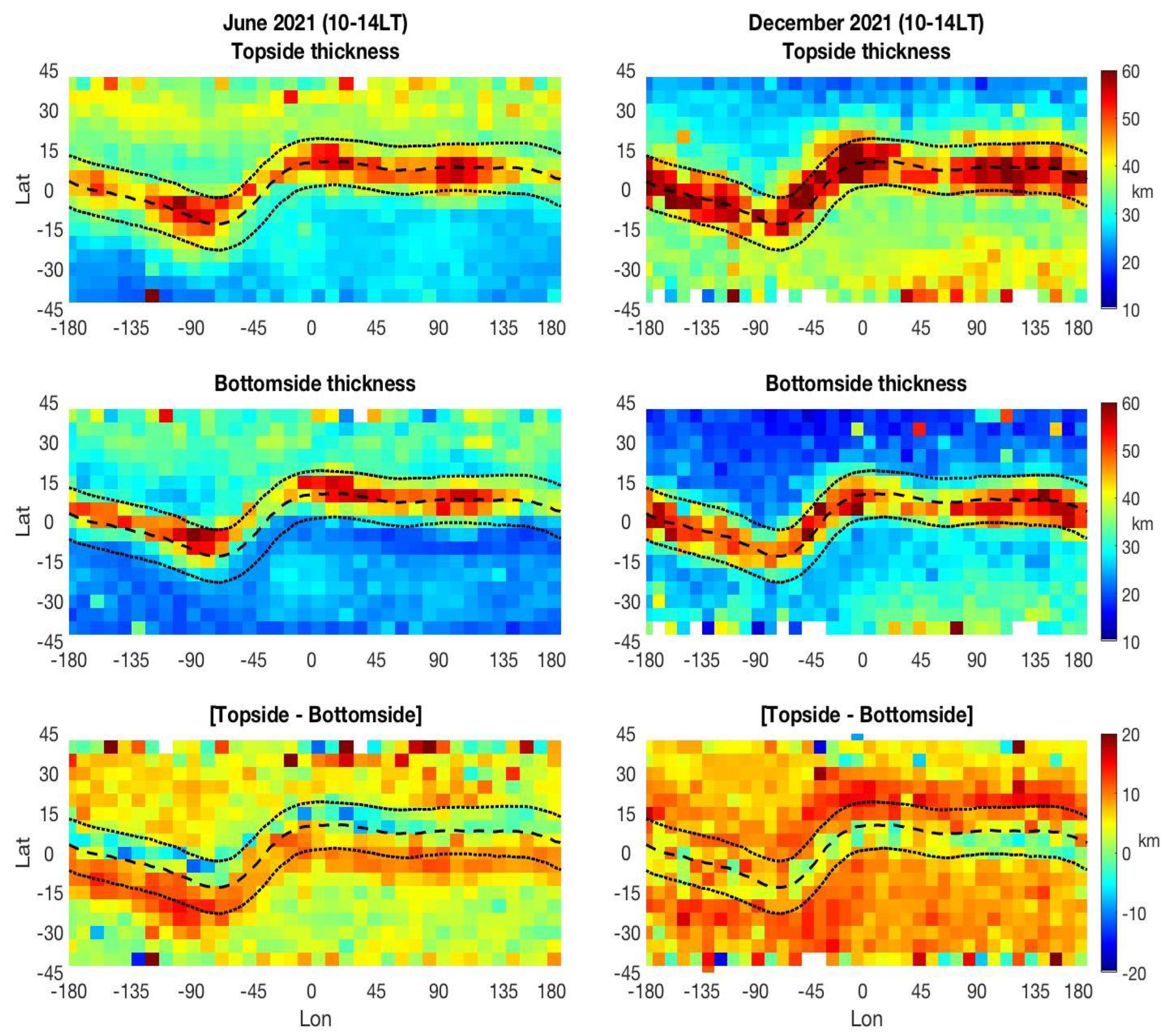
4.2. F2 Layer Thickness and the Shape of the N e Profile

Since GNSS N e retrievals are based on measurements at every altitude, they can be effectively utilized to investigate the shape of the N e profile for the topside and bottomside of the ionosphere. As an example, we estimate thicknesses of the F2 layer at 90% of NmF2 above and below the F2 peak. Figure 19 shows the top and bottom layers obtained using COSMIC-2 measurements during local 10–14 hours for June and December 2021. The topside and bottomside thicknesses are estimated using the height differences between the F2 peak (NmF2) and 90% of NmF2 in the top and bottom sides, respectively. In figure, the estimated thicknesses for June are shown on the left side and the thicknesses for December are shown on the right side. The upper panel shows the topside thicknesses and the middle panel shows the same for the bottomside. The differences between the topside and bottomside of the F2 layer (i.e., topside thickness–bottomside thickness) are shown in the bottom panel. As expected, a distinct hemispheric asymmetry is evident both in the topside and bottomside layers. In addition, a prominent longitudinal variation is also evident in both of the layers, especially along the geomagnetic equator. The F2 layer thickness appears to be modulated by the tidal component of wavenumber 4 (WN4), which is also observed in N e (see [23]). A similar but opposite hemispheric asymmetry is evident in December 2021 COSMIC-2 measurements. However, the tidal WN4 component is not prominent, as in the case of June.
The estimated thickness differences between the topside and the bottomside of the F2 layer (i.e., topside thickness–bottomside thickness) shown in the bottom panel of Figure 19 reveals another prominent feature in the N e profile. In addition to the expected seasonal variability, substantial differences are also evident between June and December. During June (left), the highest level of difference between top- and bottom-layer thicknesses is shifted toward the southern EIA crest region (bottom panel). It is prominent and consistent at all geomagnetic longitudes. This indicates that a relatively higher E × B uplift occurs during northern summer, which, in turn, affects the scale height, and hence the shape, of the topside N e profile. However, during December (right), such a prominent feature is not consistent along the northern EIA crest region at all longitudes. It is prominent only in the European and Asian sectors. Earlier, [44] showed that the variation in scale height for the topside is small, and hence, it can be assumed to be a constant scale height, and the topside N e profile can be approximated by the α -Chapman function with a constant scale height equal at hmF2. However, several subsequent studies using topside measurements indeed indicated that adaptation of height-dependent scale height is important for the topside (e.g., [45,46]). Since the ionospheric scale height is the key parameter that defines the shape of the N e profile, efforts have been made in recent years to establish the vertical N e distribution using several analytical functions such as Chapman, exponential, parabolic, and Epstein step functions ([47,48,49]). An increasing number of SmallSat/CubeSat constellations with better sampling rates provide potential opportunities to investigate the vertical N e distributions in great detail. Although the inherent assumption of spherical symmetry makes RO analysis difficult in regions of sharp gradients, GNSS-based measurements provide reliable F2 layer measurements on the global level (e.g., [32,50]), and our results further reconfirm this.

5. Concluding Summary

In this work, we evaluated and compared newly derived F-region N e retrieval profiles from an optimal estimation (OE) inversion technique with conventional onion-peeling (OP)-retrieved N e , as well as measurements from Digisondes and incoherent scatter radars (ISRs). The OE inversion algorithm was applied to COSMIC-1, COSMIC-2, and Spire constellations to retrieve N e profiles within ∼100–500 km. The estimated NmF2 and hmF2 values from OE-retrieved N e show good agreement with the OP-retrieved values. For COSMIC-1 and COSMIC-2, the best-fit agreement between the two retrieval techniques remains ∼0.9–1.0 for NmF2 and ∼0.8–0.9 for hmF2. While a higher level of agreement is evident with COSMIC-2, we were unable to compare the agreement in the case of the Spire constellation due to the unavailability of OP-retrieved N e profiles.
We also compared the OE-retrieved NmF2 and hmF2 values with ∼30 worldwide Digisonde-autoscaled NmF2 and hmF2 measurements. While good agreement is present in the NmF2 comparison (with an overall best fit of ∼0.9), a significant level of differences is evident in the case of the hmF2 comparison with all three constellations. The hmF2 differences between the two techniques depend on both the time of day and latitude. During the daytime, the Digisonde-measured hmF2 values are ∼5–25 km lower than the OE-retrieved values in the equatorial region, and the deviations further increase to ∼25–45 km in mid and high latitudes. In addition, comparisons of OE-retrieved NmF2 and hmF2 values with ISR N e measurements at two locations (Millstone Hill and Tromso) show good agreement.
Our further analysis in the observed Digisonde-autoscaled hmF2 indicates that the presence of the F1 layer during the daytime causes uncertainties in the autoscaled hmF2 values, especially when the critical frequency of the F1 layer (foF1) is relatively closer to the critical frequency of the F2 layer (foF2). During the daytime, it is noticeable that the separation between foF2 and foF1 is wider in the equatorial region and tends to become narrower at mid and high latitudes. Hence, this could be the possible cause for the observed differences between OE-retrieved and Digisonde autoscaled hmF2 values.
In addition, we also briefly showed that the estimated OE-retrieved topside and bottomside ionospheric layer thicknesses in the EIA region reflect tidal modulation of wavenumber 4. This indicates that the OE retrieval technique will be a very useful tool to investigate topside scale height and its variability, which are important for realistic reconstruction of ionospheric N e models. Our careful evaluation of OE/v6p using NmF2 and hmF2 values shows that this inversion algorithm is a good alternative for the OP retrieval of F-region N e profiles and provides unprecedented capabilities to perform comprehensive ionospheric studies.

Author Contributions

Conceptualization, N.S. and D.L.W.; methodology, N.S.; validation, N.S.; formal analysis, N.S.; investigation, N.S., D.L.W., D.J.E. and R.G.-G.; resources, D.L.W.; writing—original draft preparation, N.S. and D.J.E.; writing—review and editing, N.S., D.L.W., D.J.E. and R.G.-G. All authors have read and agreed to the published version of the manuscript.

Funding

This research was funded by NASA’s programs: Living With a Star (LWS) under WBS 936723.02.01.12.48 and Commercial Smallsat Data Acquisition (CSDA) under WBS 880292.04.02.01.68.

Data Availability Statement

The COSMIC-1 and COSMIC-2 data presented in this study are openly available at https://cdaac-www.cosmic.ucar.edu/ (last accessed on 10 July 2023); and the Spire data in this study are openly available to all US-government sponsored research at https://csdap.earthdata.nasa.gov/ (last accessed on 10 July 2023). Digisonde data are available at https://giro.uml.edu/index.html (last accessed on 15 July 2023); and radar data are available at http://cedar.openmadrigal.org/ (last accessed on 15 July 2023).

Conflicts of Interest

The authors declare no conflict of interest.

References

  1. Balan, N.; Souza, J.; Bailey, G.J. Recent developments in the understanding of equatorial ionization anomaly: A review. J. Atmos. Sol.-Terr. Phys. 2018, 171, 3–11. [Google Scholar] [CrossRef]
  2. Rishbeth, H.; Garriott, O.K. Introduction to Ionospheric Physics, 1st ed.; Academic Press: New York, NY, USA, 1969; Volume 47. [Google Scholar]
  3. Reinisch, B.W. Digisonde 4D Technical Manual (Version 1.2.11); Lowell Digisonde International: Lowell, MA, USA, 2021. [Google Scholar]
  4. Reinisch, B.W.; Huang, X. Automatic calculation of electron density profiles from digital ionograms. III—Processing of bottomside ionograms. Radio Sci. 1983, 18, 477–492. [Google Scholar] [CrossRef]
  5. Titheridge, J.E. Ionogram Analysis with the Generalised Program POLAN; Report UAG; UAG: Irvine, CA, USA, 1985; Volume 93. [Google Scholar]
  6. Roininen, L.; Laine, M.; Ulich, T. Time-varying ionosonde trend: Case study of Sodankylä hmF2 data 1957–2014. J. Geophys. Res. Space Phys. 2015, 120, 6851–6859. [Google Scholar] [CrossRef]
  7. Galkin, I.A.; Reinisch, B.W. The New ARTIST 5 for all Digisondes. Ionosonde Netw. Advis. Group Bull. 2008, 69, 1–8. [Google Scholar]
  8. Reinisch, B.W.; Galkin, I.A. Global Ionospheric Radio Observatory (GIRO). Earth Planets Space 2011, 63, 377–381. [Google Scholar] [CrossRef]
  9. Gordon, W.E. Incoherent Scattering of Radio Waves by Free Electrons with Applications to Space Exploration. Proc. IRE 1958, 46, 1824–1829. [Google Scholar] [CrossRef]
  10. Hargreaves, J.K. The Solar-Terrestrial Environment; Cambridge University Press: Cambridge, UK, 1995. [Google Scholar]
  11. Rocken, C.; Kuo, Y.H.; Schreiner, W.S.; Hunt, D.; Sokolovskiy, S.; McCormick, C. COSMIC System Description. Terr. Atmos. Ocean. Sci. 2000, 11, 021. [Google Scholar] [CrossRef]
  12. Heise, S.; Jakowski, N.; Wehrenpfennig, A.; Reigber, C.; Lühr, H. Sounding of the topside ionosphere/plasmasphere based on GPS measurements from CHAMP: Initial results. J. Geophys. Res. Lett. 2002, 29, 1699. [Google Scholar] [CrossRef]
  13. Pedatella, N.M.; Forbes, J.M.; Maute, A.; Richmond, A.D.; Fang, T.W.; Larson, K.M.; Millward, G. Longitudinal variations in the F region ionosphere and the topside ionosphere-plasmasphere: Observations and model simulations. J. Geophys. Res. Space Phys. 2011, 116, A12309. [Google Scholar] [CrossRef]
  14. Schreiner, W.S.; Sokolovskiy, S.V.; Rocken, C.; Hunt, D.C. Analysis and validation of GPS/MET radio occultation data in the ionosphere. Radio Sci. 1999, 34, 949–966. [Google Scholar] [CrossRef]
  15. Tsai, L.C.; Tsai, W.H.; Schreiner, W.S.; Berkey, F.T.; Liu, J.Y. Comparisons of GPS/MET retrieved ionospheric electron density and ground based ionosonde data. Earth Planets Space 2001, 53, 193–205. [Google Scholar] [CrossRef]
  16. Yue, X.; Schreiner, W.S.; Lei, J.; Sokolovskiy, S.V.; Rocken, C.; Hunt, D.C.; Kuo, Y.H. Error analysis of Abel retrieved electron density profiles from radio occultation measurements. Ann. Geophys. 2010, 28, 217–222. [Google Scholar] [CrossRef]
  17. Pedatella, N.M.; Yue, X.; Schreiner, W.S. An improved inversion for FORMOSAT-3/COSMIC ionosphere electron density profiles. J. Geophys. Res. Space Phys. 2015, 120, 8942–8953. [Google Scholar] [CrossRef]
  18. Tulasi Ram, S.; Su, Y.; Tsai, L.; Liu, C. A self-contained GIM-aided Abel retrieval method to improve GNSS-radio occultation retrieved electron density profiles. GPS Solut. 2016, 20, 825–836. [Google Scholar] [CrossRef]
  19. Chou, M.Y.; Lin, C.C.H.; Tsai, H.F.; Lin, C.Y. Ionospheric electron density inversion for Global Navigation Satellite Systems radio occultation using aided Abel inversions. J. Geophys. Res. Space Phys. 2017, 122, 1386–1399. [Google Scholar] [CrossRef]
  20. Wu, D.L.; Emmons, D.J.; Swarnalingam, N. Global GNSS-RO Electron Density in the Lower Ionosphere. Remote Sens. 2022, 14, 1577. [Google Scholar] [CrossRef]
  21. Lin, C.Y.; Lin, C.C.H.; Liu, J.Y.; Rajesh, P.K.; Matsuo, T.; Chou, M.Y.; Tsai, H.F.; Yeh, W.H. The Early Results and Validation of FORMOSAT-7/COSMIC-2 Space Weather Products: Global Ionospheric Specification and Ne-Aided Abel Electron Density Profile. J. Geophys. Res. Space Phys. 2020, 125, e28028. [Google Scholar] [CrossRef]
  22. Swarnalingam, N.; Wu, D.L.; Gopalswamy, N. Interhemispheric Asymmetries in Ionospheric Electron Density Responses During Geomagnetic Storms: A Study Using Space-Based and Ground-Based GNSS and AMPERE Observations. J. Geophys. Res. Space Phys. 2022, 127, e30247. [Google Scholar] [CrossRef]
  23. Wu, D.L.; Swarnalingam, N.; Emmons, D.J.; Summers, T.C. Optimal Estimation Inversion of Electron Density from GNSS-POD Limb Measurements: Part I—Algorithm Description. Remote Sens. 2023, 15, 3245. [Google Scholar]
  24. Abdu, M.A.; Alam Kherani, E.; Batista, I.S.; de Paula, E.R.; Fritts, D.C.; Sobral, J.H.A. Gravity wave initiation of equatorial spread F/plasma bubble irregularities based on observational data from the SpreadFEx campaign. Ann. Geophys. 2009, 27, 2607–2622. [Google Scholar] [CrossRef]
  25. Bilitza, D.; Altadill, D.; Truhlik, V.; Shubin, V.; Galkin, I.; Reinisch, B.; Huang, X. International Reference Ionosphere 2016: From ionospheric climate to real-time weather predictions. Space Weather 2017, 15, 418–429. [Google Scholar] [CrossRef]
  26. VanZandt, T.; Clark, W.; Warnock, J. Magnetic Apex Coordinates: A Magnetic Coordinate System for the Ionospheric F2 Laye. J. Geophys. Res. 1972, 77, 2406–2411. [Google Scholar] [CrossRef]
  27. Gilbert, J.D.; Smith, R.W. A comparison between the automatic ionogram scaling system ARTIST and the standard manual method. Radio Sci. 1988, 23, 968–974. [Google Scholar] [CrossRef]
  28. McNamara, L.F. Quality figures and error bars for autoscaled Digisonde vertical incidence ionograms. Radio Sci. 2006, 41, RS4011. [Google Scholar] [CrossRef]
  29. Enell, C.F.; Kozlovsky, A.; Turunen, T.; Ulich, T.; Välitalo, S.; Scotto, C.; Pezzopane, M. Comparison between manual scaling and Autoscala automatic scaling applied to Sodankylä Geophysical Observatory ionograms. Geosci. Instrum. Methods Data Syst. 2016, 5, 53–64. [Google Scholar] [CrossRef]
  30. Pezzopane, M.; Scotto, C. Automatic scaling of critical frequency foF2 and MUF(3000)F2: A comparison between Autoscala and ARTIST 4.5 on Rome data. Radio Sci. 2007, 42, RS4003. [Google Scholar] [CrossRef]
  31. Galkin, I.A.; Reinisch, B.W.; Huang, X.; Khmyrov, G.M. Confidence Score of ARTIST-5 Ionogram Autoscaling; INAG Technical Memorandum; INAG: Laguna Hills, CA, USA, 2013. [Google Scholar]
  32. Burns, A.G.; Solomon, S.C.; Wang, W.; Qian, L.; Zhang, Y.; Paxton, L.J. Daytime climatology of ionospheric NmF2 and hmF2 from COSMIC data. J. Geophys. Res. Space Phys. 2012, 117, A09315. [Google Scholar] [CrossRef]
  33. Kil, H.; Talaat, E.R.; Oh, S.J.; Paxton, L.J.; England, S.L.; Su, S.Y. Wave structures of the plasma density and vertical E × B drift in low-latitude F region. J. Geophys. Res. Space Phys. 2008, 113, A09312. [Google Scholar] [CrossRef]
  34. Luan, X.; Wang, P.; Dou, X.; Liu, Y.C.M. Interhemispheric asymmetry of the equatorial ionization anomaly in solstices observed by COSMIC during 2007–2012. J. Geophys. Res. Space Phys. 2015, 120, 3059–3073. [Google Scholar] [CrossRef]
  35. Krankowski, A.; Zakharenkova, I.; Krypiak-Gregorczyk, A.; Shagimuratov, I.I.; Wielgosz, P. Ionospheric electron density observed by FORMOSAT-3/COSMIC over the European region and validated by ionosonde data. J. Geod. 2011, 85, 949–964. [Google Scholar] [CrossRef]
  36. Cherniak, I.; Zakharenkova, I.; Braun, J.; Wu, Q.; Pedatella, N.; Schreiner, W.; Weiss, J.P.; Hunt, D. Accuracy assessment of the quiet-time ionospheric F2 peak parameters as derived from COSMIC-2 multi-GNSS radio occultation measurements. J. Space Weather Space Clim. 2021, 11, 18. [Google Scholar] [CrossRef]
  37. Themens, D.R.; Reid, B.; Elvidge, S. ARTIST Ionogram Autoscaling Confidence Scores: Best Practices. URSI Radio Sci. Lett. 2022, 4, 1. [Google Scholar] [CrossRef]
  38. Scotto, C.; Sabbagh, D. The Accuracy of Real-time hmF2 Estimation from Ionosondes. Remote Sens. 2020, 12, 2671. [Google Scholar] [CrossRef]
  39. Krasheninnikov, I.V.; Leshchenko, L.N. Errors in Estimating of the F2-Layer Peak Parameters in Automatic Systems for Processing the Ionograms in the Vertical Radio Sounding of the Ionosphere under Low Solar Activity Conditions. Geomagn. Aeron. 2021, 61, 703–712. [Google Scholar] [CrossRef]
  40. Stankov, S.M.; Jodogne, J.C.; Kutiev, I.; Stegen, K.; Warnant, R. Evaluation of automatic ionogram scaling for use in real-time ionospheric density profile specification: Dourbes DGS-256/ARTIST-4 performance. Ann. Geophys. 2012, 55, 283–291. [Google Scholar]
  41. McNamara, L.F.; Cooke, D.L.; Valladares, C.E.; Reinisch, B.W. Comparison of CHAMP and Digisonde plasma frequencies at Jicamarca, Peru. Radio Sci. 2007, 42, RS2005. [Google Scholar] [CrossRef]
  42. Jacobs, L.; Poole, A.W.V.; McKinnell, L.A. An analysis of automatically scaled F1 layer data over Grahamstown, South Africa. Adv. Space Res. 2004, 34, 1949–1952. [Google Scholar] [CrossRef]
  43. Pezzopane, M.; Scotto, C. A method for automatic scaling of F1 critical frequencies from ionograms. Radio Sci. 2008, 43, RS2S91. [Google Scholar] [CrossRef]
  44. Reinisch, B.W.; Huang, X. Deducing topside profiles and total electron content from bottomside ionograms. Adv. Space Res. 2001, 27, 23–30. [Google Scholar] [CrossRef]
  45. Luan, X.; Liu, L.; Wan, W.; Lei, J.; Zhang, S.R.; Holt, J.M.; Sulzer, M.P. A study of the shape of topside electron density profile derived from incoherent scatter radar measurements over Arecibo and Millstone Hill. Radio Sci. 2006, 41, RS4006. [Google Scholar] [CrossRef]
  46. Tulasi Ram, S.; Su, S.Y.; Liu, C.H.; Reinisch, B.W.; McKinnell, L.A. Topside ionospheric effective scale heights (HT) derived with ROCSAT-1 and ground-based ionosonde observations at equatorial and midlatitude stations. J. Geophys. Res. Space Phys. 2009, 114, A10309. [Google Scholar] [CrossRef]
  47. Themens, D.R.; Jayachandran, P.T.; Bilitza, D.; Erickson, P.J.; Haggstrom, I.; Lyashenko, M.V.; Reid, B.; Varney, R.H.; Pustovalova, L. Topside Electron Density Representations for Middle and High Latitudes: A Topside Parameterization for E-CHAIM Based On the NeQuick. J. Geophys. Res. Space Phys. 2018, 123, 1603–1617. [Google Scholar] [CrossRef]
  48. Pignalberi, A.; Pietrella, M.; Pezzopane, M.; Nava, B.; Cesaroni, C. The Ionospheric Equivalent Slab Thickness: A Review Supported by a Global Climatological Study Over Two Solar Cycles. Space Sci. Rev. 2022, 218, 37. [Google Scholar] [CrossRef]
  49. Bilitza, D.; Pezzopane, M.; Truhlik, V.; Altadill, D.; Reinisch, B.W.; Pignalberi, A. The International Reference Ionosphere Model: A Review and Description of an Ionospheric Benchmark. Rev. Geophys. 2022, 60, e2022RG000792. [Google Scholar] [CrossRef]
  50. Shubin, V.N.; Karpachev, A.T.; Tsybulya, K.G. Global model of the F2 layer peak height for low solar activity based on GPS radio-occultation data. J. Atmos. Sol.-Terr. Phys. 2013, 104, 106–115. [Google Scholar] [CrossRef]
Figure 1. A comparison of OE (red) and OP (black) retrieved N e profiles at two geographical locations derived from COSMIC-1 and COSMIC-2 measurements. While the two profiles reasonably agree in the F-region, occasional differences are evident at low altitudes. In the case of OP retrieval, the left side shows an example of a monotonically increasing N e profile in E-region, whereas the right side shows an example of negative N e values in lower F- and upper E-regions.
Remotesensing 15 04048 g001
Figure 2. Initial (blue) and smoothed (red) OE-retrieved F-region N e profile from the Spire constellation during June 2021.
Remotesensing 15 04048 g002
Figure 3. Locations of the Digisonde stations used in this study. The geomagnetic equator and ±10 geomagnetic latitudes at an altitude of 350 km (based on apex geomagnetic coordinates) are marked by dashed and dotted lines, respectively.
Remotesensing 15 04048 g003
Figure 4. Comparison of global NmF2 maps from COSMIC-1 during June 2008. The left column shows OE-retrieved NmF2 values, and the middle column shows OP-retrieved NmF2 values at 00–04 UT (upper row), 10–14 UT (middle row), and 16–20 UT (bottom row). The right column shows scatter plots between the two retrieved NmF2 values for local midday (10–14 LT) and midnight (22–02 LT) hours for the respective universal time intervals.
Remotesensing 15 04048 g004
Figure 5. Comparison of global NmF2 maps from COSMIC-2 during June 2021. The left column shows OE-retrieved NmF2 values and the middle column shows OP-retrieved NmF2 values at 00–04 UT (upper row), 10–14 UT (middle row), and 16–20 UT (bottom row). The right column shows scatter plots between the two retrieved NmF2 values for local midday (10–14 LT) and midnight (22–02 LT) hours for the respective universal time intervals.
Remotesensing 15 04048 g005
Figure 6. Comparison of global hmF2 maps from COSMIC-1 during June 2008. The left column shows OE-retrieved hmF2 values and the middle column shows OP-retrieved NmF2 values at 00–04 UT (upper row), 10–14 UT (middle row), and 16–20 UT (bottom row). The right column shows scatter plots between the two retrieved NmF2 values for local midday (10–14 LT) and midnight (22–02 LT) hours for the respective universal time intervals.
Remotesensing 15 04048 g006
Figure 7. Comparison of global hmF2 maps from COSMIC-2 during June 2021. The left column shows OE-retrieved hmF2 values and the middle column shows OP-retrieved hmF2 values at 00–04 UT (upper row), 10–14 UT (middle row), and 16–20 UT (bottom row). The right column shows scatter plots between the two retrieved hmF2 values for local midday (10–14 LT) and midnight (22–02 LT) hours for the respective universal time intervals.
Remotesensing 15 04048 g007
Figure 8. Maps of NmF2 (upper panel) and hmF2 (lower panel) obtained by applying the OE retrieval technique to the Spire GNSS-POD limb measurements during local 10–14 hours in June 2021.
Remotesensing 15 04048 g008
Figure 9. Latitudinal variation of hourly NmF2 means from OE retrieval (red) and Digisonde measurements (green) are plotted in geomagnetic coordinates. The left column compares OE retrieval to Digisonde from COSMIC-1 during June 2011/2012. The middle and right columns compare COSMIC-2 and Spire to Digisonde during June 2021. Rows are separated by local time intervals from full day on the top, local midday hours (10–14 LT) in the middle, and local midnight hours (22–02 LT) in the bottom.
Remotesensing 15 04048 g009
Figure 10. Latitudinal variation of hourly hmF2 means from OE retrieval (red) and Digisonde measurements (blue) are plotted in geomagnetic coordinates. The left column compares OE retrieval to Digisonde from COSMIC-1 during June 2011/2012. The middle and right columns compare COSMIC-2 and Spire to Digisonde during June 2021. Rows are separated by local time intervals from full day on the top, local midday hours (10–14 LT) in the middle, and local midnight hours (22–02 LT) in the bottom.
Remotesensing 15 04048 g010
Figure 11. Scatter plots of NmF2 (top row) and hmF2 (bottom row) for the OE retrieval and Digisonde measurements at ∼30 global Digisonde locations for COSMIC-1 (left column), COSMIC-2 (middle column), and Spire (right column). The local time intervals of 0–24 LT hours, 22–02 LT hours, and 10–14 LT hours are marked by blue, cyan, and red dots, respectively.
Remotesensing 15 04048 g011
Figure 12. A comparison of diurnal sensitivity of NmF2 at six selected Digisonde stations using Digisonde measurements and OE and OP retrievals from COSMIC-1, COSMIC-2, and Spire during June 2012 and June 2021. See text for detailed descriptions.
Remotesensing 15 04048 g012
Figure 13. A comparison of diurnal sensitivity of hmF2 at six selected Digisonde stations using Digisonde measurements and OE and OP retrievals from COSMIC-1, COSMIC-2, and Spire during June 2012 and June 2021. See text for detailed descriptions.
Remotesensing 15 04048 g013
Figure 14. Left: Examples of F-region N e profiles at Millstone Hill from OE retrieval (red), OP retrieval (red and dashed black), and radar measurement (blue dots) are shown for 16 March 2007 (see text for details). Right upper panel: Comparison of radar measured hmF2 diurnal sensitivity with OE retrieval from COSMIC-1 and Digisonde measurements at Millstone Hill during June 2012. Right lower panel: Comparison of radar-measured hmF2 diurnal sensitivity with OE retrieval from Spire and Digisonde measurements at Tromso during March 2022.
Remotesensing 15 04048 g014
Figure 15. Contour plots of F-region N e at Millstone Hill using OE retrieval from COSMIC-1 (upper panel) and ISR measurements (lower panel) during June 2011/2012.
Remotesensing 15 04048 g015
Figure 16. OE-retrieved F2 layer thicknesses at three locations: Chilton (top panel), Fortaleza (middle panel), and Hermanus (bottom panel). The F2 layer thickness (dashed line) is considered at 95% of NmF2 above and below the mean values of hmF2 (solid red), and is plotted with Digisonde-measured mean hmF2 (black).
Remotesensing 15 04048 g016
Figure 17. Digisonde-measured daytime foF2 (green) and foF1 (red) values at three locations: Chilton (top panel), Fortaleza (middle panel), and Hermanus (bottom panel). The black line refers to hourly mean values.
Remotesensing 15 04048 g017
Figure 18. Left: Latitudinal variation of Digisonde-measured mean foF2 (green) and mean foF1 (red) during local 10–14 hours in June 2021. Right: Scatter plot of hourly (foF2–foF1) differences versus hmF2 differences between OE retrieval (Spire) and Digisonde measurements at these locations for local noon (red) and 10–14 hours (blue).
Remotesensing 15 04048 g018
Figure 19. OE-retrieved thicknesses of the F2 layer at 90% of NmF2 using COSMIC-2 measurements during local 10–14 hours in June (left) and December (right) 2021. The upper panel shows topside thickness and the middle panel shows the bottomside thickness. The difference between these two layers is shown in the bottom panel.
Remotesensing 15 04048 g019
Table 1. A comparison of statistics for OE- and OP-retrieved N e at selected low ionospheric altitudes. The means and standard deviations are estimated based on the COSMIC-2 global observations in local 11–13 hours during 1–10 December 2021. The number of available samples in each category is shown in brackets. See text for additional details.
Height (km)Optimal Estimation
Mean / Std (m−3)
Onion Peeling
Mean and Std (m−3)
1501.7 × 10 11 /1.0× 10 11 (5998)2.2 × 10 11 /1.2 × 10 11 (3788)
1208.5 × 10 10 /7.1 × 10 10 (5998)1.3 × 10 11 / 1.2 × 10 11 (3751)
1002.7 × 10 10 /1.3 × 10 10 (5998)9.1 × 10 10 /1.0 × 10 11 (3596)
903.2 × 10 09 /1.9 × 10 09 (5998)−6.8 × 10 09 /9.5 × 10 10 (3542)
Disclaimer/Publisher’s Note: The statements, opinions and data contained in all publications are solely those of the individual author(s) and contributor(s) and not of MDPI and/or the editor(s). MDPI and/or the editor(s) disclaim responsibility for any injury to people or property resulting from any ideas, methods, instructions or products referred to in the content.

