Sensitivity Evaluation of Time Series InSAR Monitoring Results for Landslide Detection

Abstract

Spaceborne interferometric synthetic aperture radar (InSAR) techniques are important for landslide detection and monitoring; however, several limitations and uncertainties, such as the unique north–south flying direction and side-look radar observing geometry, currently limit the ability of InSAR to credibly detect landslides, especially those related to high and steep slopes. Here, we conducted experimental and statistical analysis on the feasibility of time-series InSAR monitoring for steep slopes using ascending and descending SAR images. First, the theoretical (T_GNSS), practical (P_GNSS), and terrain (H_terrain) (T-P-H) indices for sensitivity evaluations of the slope displacement monitoring results from time-series InSAR were proposed for slope monitoring. Subsequently, two experimental and statistical studies were conducted for the cases with and without Global Navigation Satellite System (GNSS) monitoring data. Our experimental results of two high and steep open-pit mines showed that the defined theoretical and practical sensitivity indices can quantitatively evaluate the feasibility of ascending and descending InSAR observations in steep-slope deformation monitoring with GNSS data, and the terrain sensitivity index can qualitatively evaluate the feasibility of landslide monitoring results from ascending and descending Sentinel-1 satellite data without GNSS data. We further demonstrate the generalizability of these proposed indices using four landslide cases with both public GNSS and InSAR monitoring data and 119 landslide cases with only InSAR monitoring data. The statistical results indicated that greater indices correlated with higher reliability of the monitoring results, suggesting that these novel indices have wide suitability and applicability. This study can help to improve the practice of slope deformation monitoring using spaceborne InSAR, especially for high and steep slopes.

1. Introduction

Landslides are complex and common geohazards that can lead to global property damage and casualties [1,2,3]. Landslides in open-pit mines occur as a result of slope destabilization due to slope damage, which is caused by a variety of factors in the man-made mining process. The landslide types occurring in open-pit mines are mainly rotational landslide, translational landslide, block slide, topple, and composite landslides, and their prevention requires effective and early detection, monitoring, and warning techniques [4,5]. Currently, in situ measurements and remote sensing methods are widely used for landslide monitoring, including total station monitoring, measurement robot monitoring, GNSS real-time monitoring, laser scanner monitoring, high-resolution optical image monitoring, thermal infrared monitoring, and spaceborne InSAR monitoring [6]. Spaceborne InSAR is typically precise and has high resolution and continuous space coverage, while being capable of continuous all-weather operation [7,8]. Initially, the differential InSAR (D-InSAR) method was used to carry out deformation monitoring. However, the complex topographic environment, dense vegetation cover, and severe atmospheric influence in the landslide monitoring region of an open-pit mine, result in the D-InSAR method more seriously affected by temporal and spatial decoherence and atmospheric delay, etc. In addition, due to the unique flight mode of SAR satellites (north–south flight), the monitoring capability of D-InSAR for north–south deformation is weak, and these shortcomings lead to the relatively low-precision deformation monitoring results of D-InSAR technology in the open-pit mine [9]. In 2002, small baseline subset differential interferometry (SBAS-InSAR) technology was proposed and used to obtain the time-series surface deformation of the Campi Flegrei crater and Naples city. This method has been shown to accurately estimate time-series deformations [10]. Compared with persistent scatterer synthetic aperture radar interferometry (PS-InSAR) technology [11], SBAS-InSAR uses a short baseline combination for interferometry, which overcomes the poor coherence of interferograms that PS-InSAR suffers from by using long spatial or temporal baselines, the necessity of a large-scale number of SAR images (typically > 20), and low operation efficiency [12]; therefore, SBAS-InSAR has improved the accuracy of deformation monitoring of time-series InSAR in open-pit mine regions [13,14]. Furthermore, some studies have shown that SBAS-InSAR technology is more suitable for deformation monitoring in field areas with more rapid surface motion than PS-InSAR technology [15,16]. This study utilized SBAS-InSAR to monitor the slope deformation in the Qidashan and Yabaling open-pit mines and obtained the time-series deformation and displacement rates of the slopes.

Owing to the side-looking radar imaging geometry and unique north–south flying direction of the satellite SAR system, the surface deformation monitored by InSAR is only one-dimensional deformation that is along the line of sight (LOS) direction, rather than the actual three-dimensional deformation of the surface in the up–down, east–west, and north–south directions [17,18]. Additionally, an abundance of SAR images are used for time-series InSAR, rendering it is beneficial to assess the monitoring sensitivity of InSAR prior to heavy and abundant data processing; therefore, many scholars have studied the feasibility of InSAR monitoring. For example, Cascini et al. [19] pioneered the concept of using “visibility maps” for landslides, but did not consider the geometric distortion caused by terrain factors including shadow, layover, and foreshortening. The “R-Index” was later proposed by Notti et al. [20], which estimates the feasibility of InSAR based on terrain geometry, and a series of improved studies were subsequently conducted [21,22,23]. Recently, the “P-NG” method was proposed to determine the magnitude of geometric distortion as it can distinguish more types of geometric distortion [24,25]; however, these studies did not consider landslide deformation patterns [26], especially those high and steep landslides, for example, the slope height greater than 200 m and slope angle greater than 42 degrees.

Overall, few studies have quantitatively evaluated the reliability of time-series InSAR displacement monitoring results for high and steep slopes based on the sensitivity of different SAR orbits, which restricts the effective application of the time-series InSAR method in landslide monitoring of large open-pit mines. The displacement along the sliding direction can be used as the benchmark parameter to quantitatively evaluate the reliability of landslides monitored by time-series InSAR because the slope gradient of a high and steep open-pit is a critical factor causing landslides, and the slope is highly consistent with the sliding angle. Combined with InSAR monitoring results and high-precision digital elevation model (DEM) data, we defined the theoretical sensitivity index (T_GNSS) and practical sensitivity index (P_GNSS) of slope monitoring sensitivity based on GNSS monitoring results, which were used as the reliability evaluation index for the quantitative evaluation of InSAR slope displacement monitoring results. For the scenario without GNSS monitoring results, we further defined the terrain sensitivity index (H_terrain) by combining the geometric characteristics of slope displacement with the relationship between slope displacement and SAR observation geometry. Finally, using the Qidashan and Yabaling open-pit mines as experimental cases, we analyzed and verified the availability and effectiveness of Sentinel-1 satellite data to identify and monitor landslides. Then, using four landslide cases with GNSS monitoring data and 119 landslide cases without GNSS monitoring data, we statistically analyzed the proposed sensitivity indices for slope monitoring in all cases and proved the general adaptability of the new indices.

2. Locations and Datasets of Two High and Steep Slopes

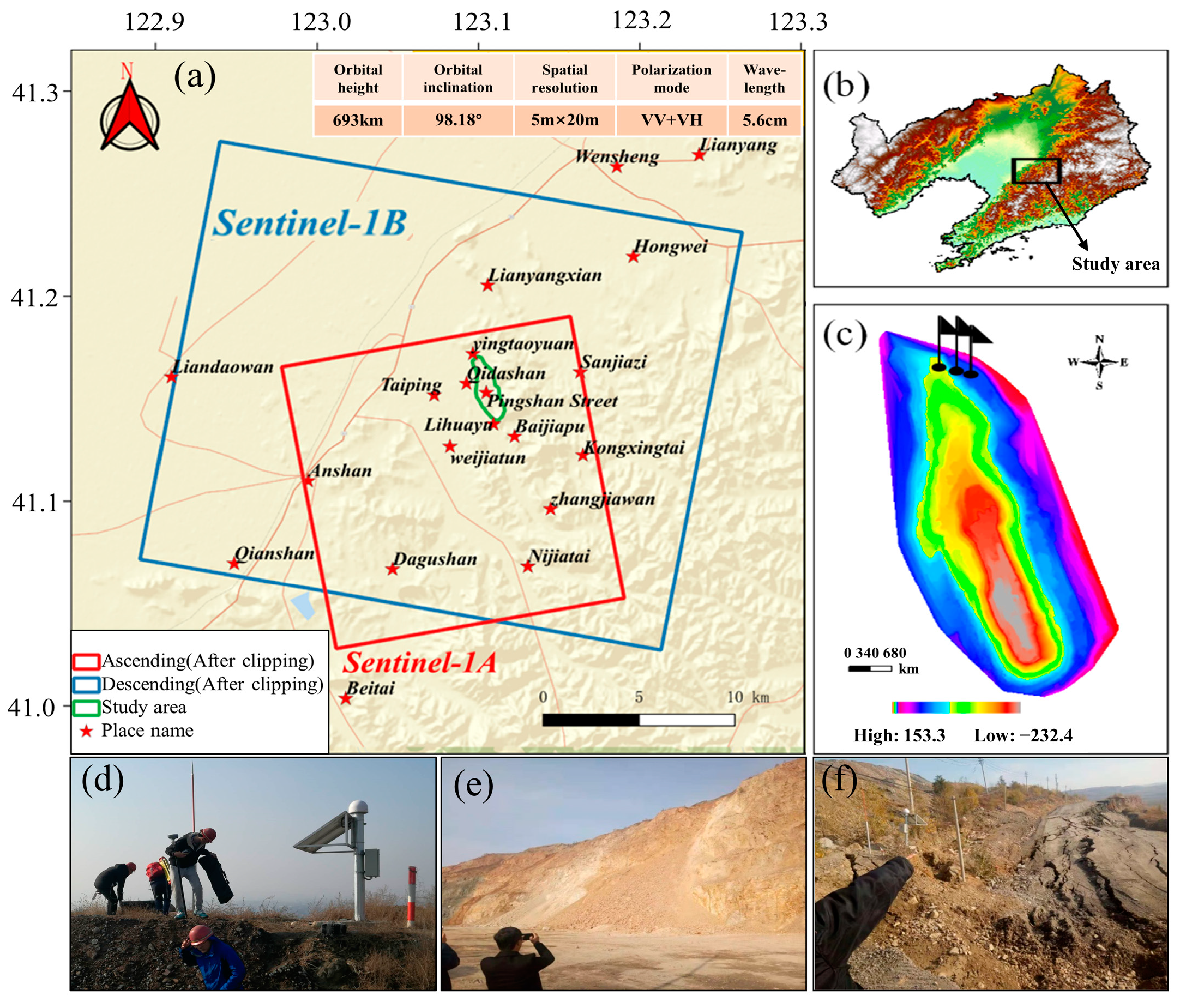
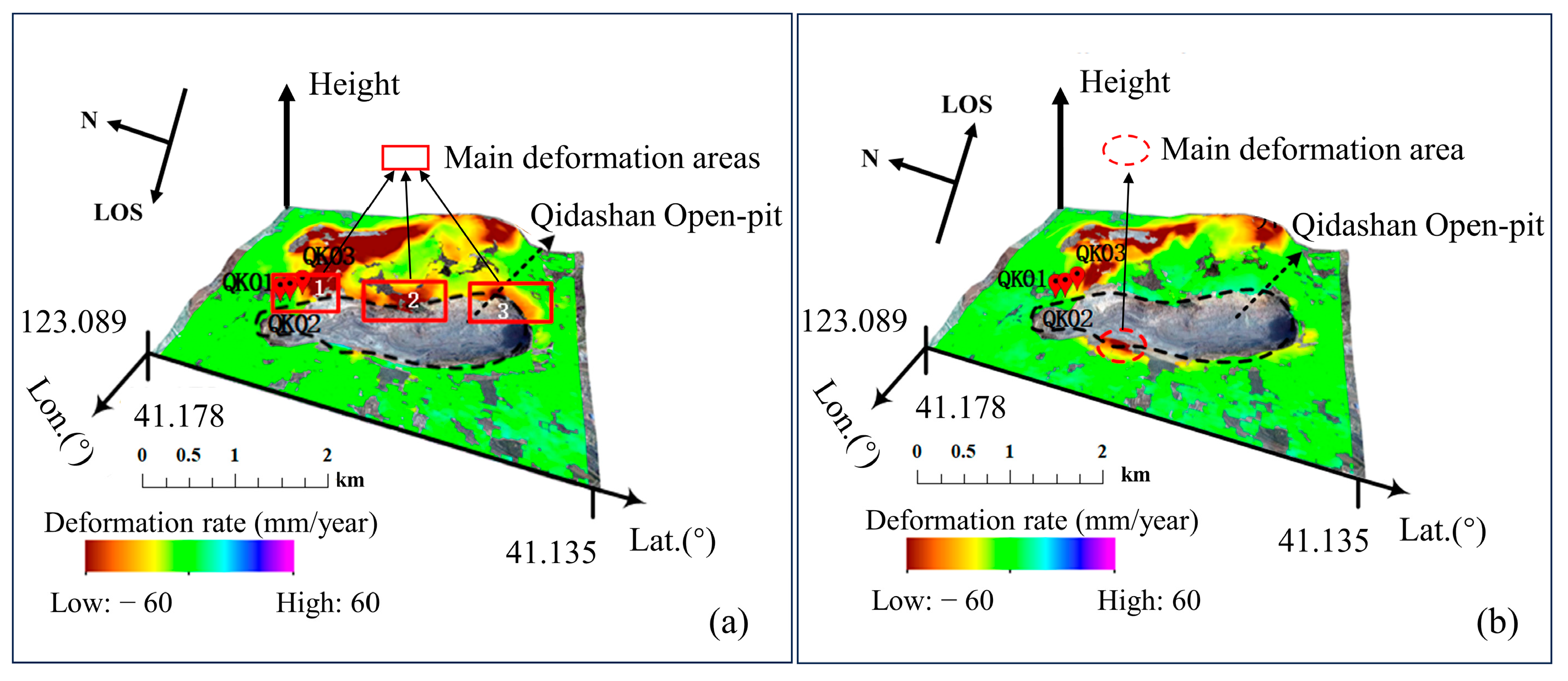
2.1. Location and SAR Datasets of the Qidashan Open-Pit Mine Landslide

First, we considered the high and steep slope of the Qidashan open-pit mine, the largest open-pit metal mine in Asia, located in the northeast of Anshan City, Liaoning Province, China, as an experimental study. This metal mine is composed of an open pit and several tailing reservoirs covering 1121 hectares, and the open-pit mine is 3400 m long, 1000 m wide, and 230 m deep (Figure 1). Long-term, high-intensity, and large-scale continuous mining makes slopes extremely unstable, which leads to increasing landslide disasters. Rapid and accurate monitoring and timely and effective early warnings are crucial for mine disaster prevention and reduction.

Slope deformation monitoring of the Qidashan open-pit mine was conducted by combining the SBAS-InSAR and GNSS real-time monitoring techniques. The red and blue quadrangles in Figure 1a are the coverage areas of the ascending and descending orbit radar satellite images after clipping, and the green area in Figure 1a is the study area of the Qidashan open-pit mine. Figure 1b shows a topographic map of Liaoning Province, and Figure 1c shows the high-precision DEM data of the Qidashan open-pit mine generated from point cloud data obtained using a three-dimensional laser scanning system. Sentinel-1 SAR data from European Space Agency were utilized in this study, and the detailed parameters are listed in

Table 1. Detailed parameters of the Sentinel-1 satellite data for the slope deformation monitoring of the Qidashan open-pit mine.

Satellite	Orbit	Incidence Angle (°)	Heading Angle (°)	Period	Number of Scenes	Maximum Spatial Baseline (m)	Resolution Azimuth × Range (m2)
Sentinel-1A	Ascending	33.7	−13.54	22 October 2018–14 May 2019	18	83.4	5 m × 20 m
Sentinel-1B	Descending	36.1	166.37	26 October 2018–18 May 2019	17	135.6	5 m × 20 m

. Additionally, three continuously operating GNSS monitoring stations, noted by the black flags in Figure 1c, were installed in the region with a large deformation in the northeastern part of the open-pit mine. From left to right, these monitoring stations are QK01, QK02, and QK03, respectively. Three-dimensional high-precision deformation data from these GNSS stations were obtained. The horizontal accuracy was better than 2 mm and the vertical accuracy was better than 4 mm for the three GNSS sites.

We processed two datasets of 18 Sentinel-1A ascending SAR images and 17 Sentinel-1B descending SAR images of the C-band in interferometric wide swath mode. The ascending data span from 22 October 2018 to 14 May 2019, with a maximum spatial baseline of 83.4 m and an average spatial baseline of 19.27 m. The time interval of descending data was from 26 October 2018 to 18 May 2019, the maximum spatial baseline was 135.6 m, and the average spatial baseline was 21.93 m.

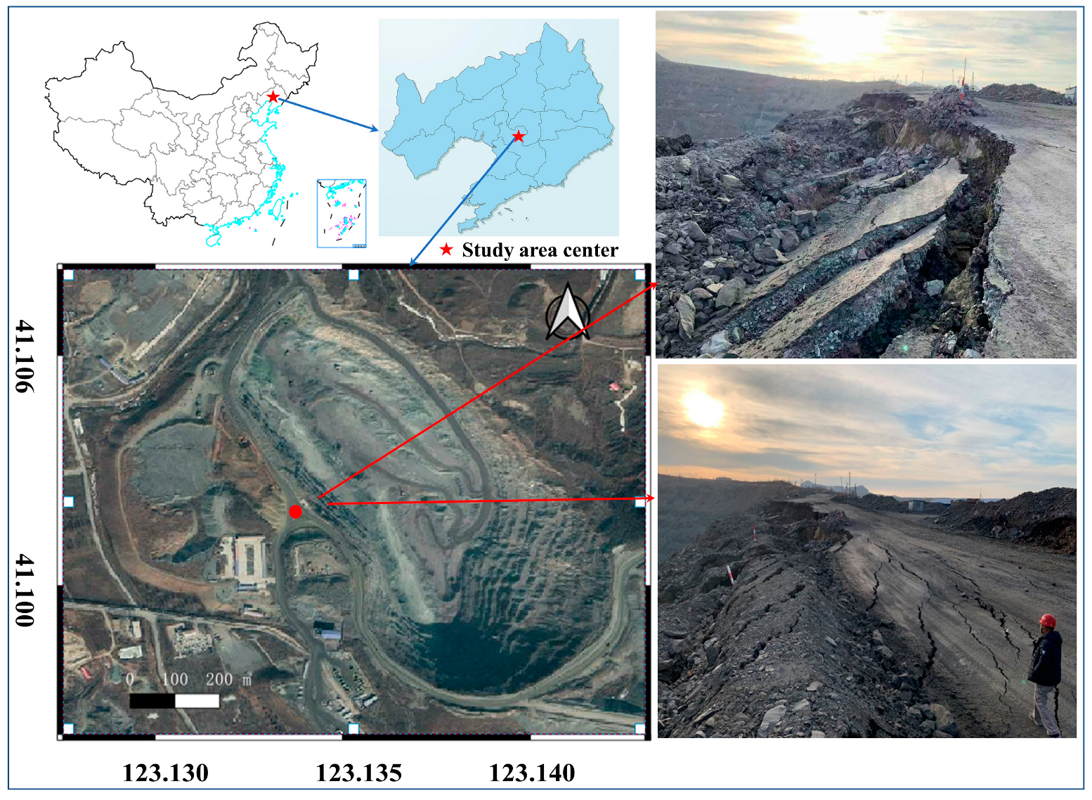
2.2. Location and SAR Datasets of the Yabaling Open-Pit Mine Landslide

The second case was that of the Yabaling open-pit mine, which is also located in the eastern part of Anshan City, Liaoning Province, China. A landslide occurred on 25 November 2019 in the Yabaling open-pit mine, as shown in Figure 2. Owing to long-term continuous mining, the Yabaling open-pit mine has turned into deep concave open-pit mining, forming many landslide-prone hazard areas.

In this study, Sentinel 1A/B TOPS C-band SAR images were used to map the time-series deformation of the slopes of the Yabaling open-pit mine. Overall, 29 SLC images of ascending orbit (including two orbits: T25 and T98) in interferometric wide mode were collected from 7 June 2019, to 22 November 2019, and 15 SLC images of descending orbit (T105) in interferometric wide mode were collected from 6 June 2019 to 21 November 2019. Detailed information on the Sentinel-1 SAR data is presented in

Table 2. Detailed parameters of the Sentinel-1 data.

Satellite	Orbit	Incidence Angle (°)	Heading Angle (°)	Period	Number of Scenes
Sentinel-1A	Ascending1 (T25)	38.87	−13.53	7 June 2019–22 November 2019	14
Sentinel-1A	Descending (T98)	38.86	−13.53	12 June 2019–15 November 2019	15
Sentinel-1B	Descending (T105)	39.02	166.42	6 June 2019–21 November 2019	15

.

3. Definition of Sensitivity Indices for Slope Monitoring

Over the past two decades, time-series InSAR has become capable of reducing temporal and geometrical decorrelations using multiple SAR images. SBAS-InSAR is a widely used time-series InSAR method that has high coherence of interferograms and mitigation of irregular atmospheric delays and can focus on coherent radar targets instead of the ensemble of image pixels [27]. Therefore, we utilized this method to process all relevant available SAR images. First, we selected the appropriate spatio-temporal baseline thresholds to combine image pairs from multiple SAR images arranged chronologically covering the study area [28]. Then, according to the connection relationship, all the image pairs were processed by interferometric, flattening, filtering, and phase unwrapping to obtain the interferogram. The topographic and residual phases were then estimated and corrected by introducing external DEM data and ground control points (GCP) [29], the selection of which in the open-pit mining areas were not located in the residual terrain phase of high frequency, deformation phase, and break phase, and were located in a relatively stable nondeformed region [30]. The interferogram was then reflected and refined. Next, the minimum-cost flow method was used for phase unwrapping [31], and the time-series surface displacement was estimated using the singular-value decomposition method. Finally, geocoding was performed to obtain the cumulative surface deformation and deformation rates in the WGS-84 coordinate system.

The visibility of the surface of the Earth to radar satellite sensors depends on the parameters of the satellite and the terrain geometry; therefore, in different parts of the same SAR image, the change in the detectability sensitivity depends on the local incident angle, which is determined by the aspects of the local terrain slope. Considering these effects, slant-range geometrical distortions can be classified as layover, foreshortening, and shadows [32], and the existence of geometrical distortions considerably limits the application of InSAR [33]; therefore, prior knowledge is required to determine the detectability of the study area. Based on the multi-orbit datasets, combined with obtained terrain information, the most appropriate SAR monitoring data were evaluated to ensure that the study area can be sufficiently monitored to save a lot of time and cost and achieve efficient monitoring.

As shown in Figure 3, the deformation directly observed by InSAR is not the deformation of the ground, but the deformation along the LOS direction, which is the superposition of deformation projections in the north–south (N), east–west (E), and up–down (U) displacements. Sentinel-1 is a near-polar-orbiting satellite; therefore, it is not sensitive to north–south deformation [34].

By combining InSAR displacements from two imaging geometries, that is, one ascending and one descending geometry, the three-dimensional InSAR surface displacement was calculated. The InSAR LOS displacement derived from ascending orbit data $S_{Los}^A$ consists of a ground vector D_R (LOS projection in the horizontal direction) and a vertical vector D_U, as follows:

$$S_{LoS}^A=D_U\cdot \mathit{cos}{\theta }^A+D_R\cdot \mathit{sin}{\theta }^A$$

(1)

where ${\theta }^A$ represents the incidence angle of ascending orbit image.

The ground displacement vector $D_R$ consists of the eastern displacement vector $D_E$ and southern displacement vector $D_N$ as follows:

$$D_R=D_E\cdot \left(-\mathit{sin}\left({\gamma }^A-3\pi /2\right)\right)+D_N\cdot \left(-\mathit{cos}\left({\gamma }^A-3\pi /2\right)\right)$$

(2)

where ${\gamma }^A$ is the orbit azimuth angle of the ascending orbit image, which is the angle between the north and satellite flight directions (clockwise). Substituting Equation (2) into Equation (1), the relationship between the LOS direction deformation vector and the three-dimensional surface deformation vector for the ascending orbit data is obtained as follows:

$$S_{LOS}^A=D_U\cdot \mathit{cos}{\theta }^A-D_E\cdot \mathit{sin}{\theta }^A\cdot \mathit{cos}{\gamma }^A+D_N\cdot \mathit{sin}{\theta }^A\cdot \mathit{sin}{\gamma }^A$$

(3)

Similarly, the relationship between the LOS direction displacement vector and the three-dimensional surface displacements vector for the descending orbit data is as follows:

$$S_{LOS}^D=D_U\cdot \mathit{cos}{\theta }^D-D_E\cdot \mathit{sin}{\theta }^D\cdot \mathit{cos}{\gamma }^D+D_N\cdot \mathit{sin}{\theta }^D\cdot \mathit{sin}{\gamma }^D$$

(4)

By setting X = −sin α·cos β; Y = sin α·sin β; and Z = cos α, Equations (3) and (4) were rewritten into the following matrix:

$$\left[\begin{array}{c}{S}_{LOS}^A\\ S_{LOS}^D\end{array}\right]=\left[\begin{array}{ccc}{X}_A& Y_A& Z_A\\ X_D& Y_D& Z_D\end{array}\right]\left[\begin{array}{c}{D}_E\\ D_N\\ D_U\end{array}\right]$$

(5)

where $\left[\begin{array}{ccc}X& Y& Z\end{array}\right]$ is called the vector projection of InSAR LOS in the three-dimensional directions of ENU [35,36]. Superscripts A and D denote ascending and descending orbits, respectively.

3.1. Definition of Theoretical and Practical Sensitivity Indices Based on GNSS Data

When GNSS deformation monitoring data of the open-pit mine slope were available, the displacements of the slope in three-dimensional directions were provided by the GNSS real-time monitoring station. Subsequently, the geometric parameters of the ascending and descending orbit satellites are substituted into Equation (5) to calculate the LOS deformation of the open-pit mine slope displacement vector under ascending and descending orbit conditions.

Landslides are generally displaced along the slope direction, so it is necessary to convert the displacement in the three-dimensional direction to the slope direction, and combine the two parameters of slope angle (φ) and aspect angle (α) to establish the expression of slope direction displacement ($S_{Slope}$) as follows:

$$S_{Slope}=D_U\cdot \mathit{sin}\phi -D_E\cdot \mathit{sin}\alpha \cdot \mathit{cos}\phi -D_N\cdot \mathit{cos}\alpha \cdot \mathit{cos}\phi$$

(6)

To quantitatively evaluate the reliability of InSAR deformation results in open-pit mine slope monitoring, the theoretical sensitivity index (T_GNSS) and practical sensitivity index (P_GNSS) slope monitoring were defined by combining aspect angle (α) and slope angle (φ), and the calculation formulae were as follows:

$$\left[\begin{array}{c}{T}_{GNSS}^A\\ T_{GNSS}^D\end{array}\right]=\left[\begin{array}{c}{S}_{LOS}^A/S_{Slope}\\ S_{LOS}^D/S_{Slope}\end{array}\right]\times 100\%$$

(7)

$$\left[\begin{array}{c}{P}_{GNSS}^A\\ P_{GNSS}^D\end{array}\right]=\left[\begin{array}{c}{I}_{LOS}^A/S_{Slope}\\ I_{LOS}^D/S_{Slope}\end{array}\right]\times 100\%$$

(8)

where $S_{Los}^A$ and $S_{Los}^D$ are the LOS projection deformations of GNSS under the conditions of ascending and descending orbits, respectively; $S_{Slope}$ is the deformation of GNSS in the slope direction; and $I_{Los}^A$ and $I_{Los}^D$ are the LOS deformations obtained by InSAR for ascending and descending orbits, respectively.

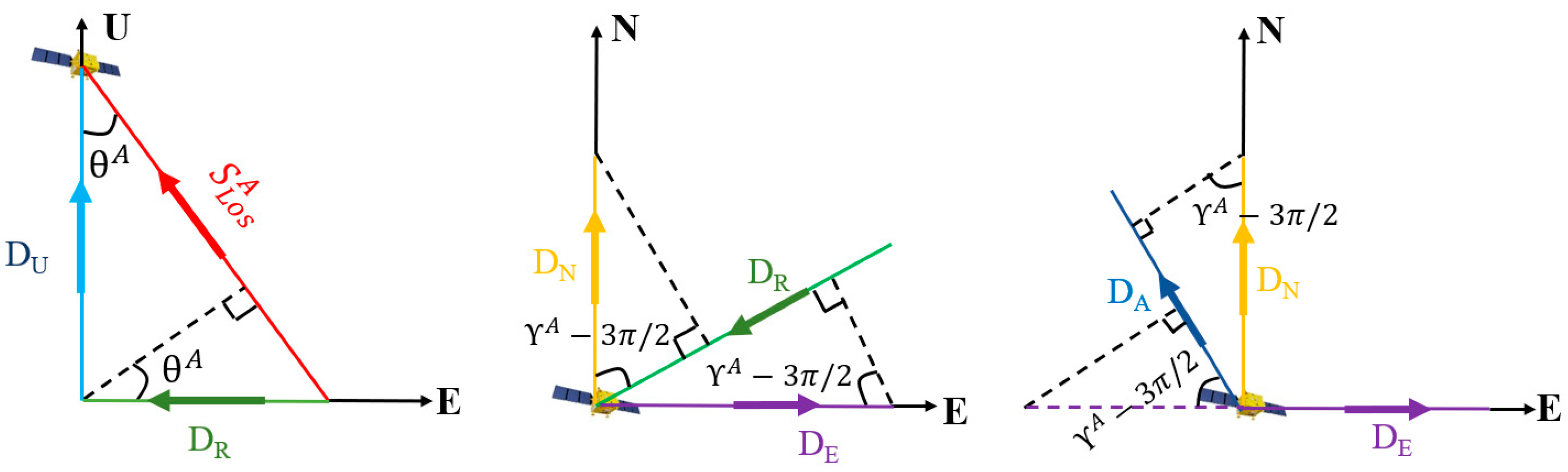
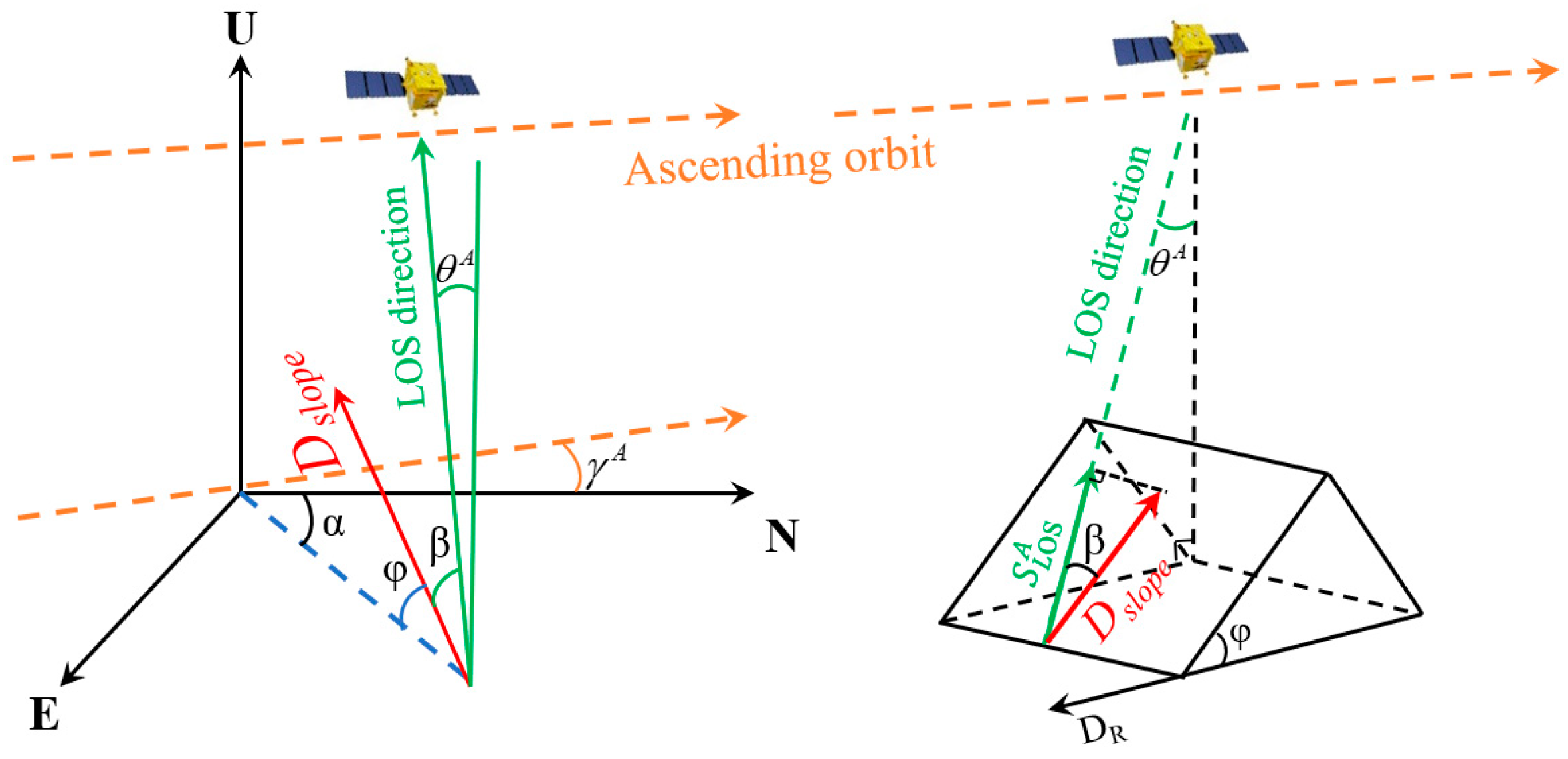
3.2. Definition of Terrain Sensitivity Index through Satellite and Terrain Information

The high cost of GNSS monitoring equipment and the uncertainty of which areas are potential landslide regions can make it difficult to obtain GNSS deformation monitoring data; therefore, we could not obtain the true slope-slip deformation. To accommodate these problems, we defined the terrain sensitivity index by combining the imaging geometry of the SAR satellite with local terrain parameters. Publicly available high-precision DEM data were used to obtain terrain information such as slope and aspect, and the two study areas involved in this study have LiDAR point cloud data from which slope and aspect information can be accurately obtained.

Generally, the deformation along the LOS direction derived from InSAR is insufficient for reflecting the deformation of the slope [37,38]. Figure 4 shows the typical imaging geometry of the ascending orbit, where φ is the slope angle, α is the aspect angle, and β is the angle between vector $S_{Los}^A$ and vector D_Slope. We decomposed vector D_Slope into three directions, that is, N, E, and U [39], and the decomposition result is expressed as a matrix in Equation (9).

$$\left[\begin{array}{c}{D}_U\\ D_N\\ D_E\end{array}\right]=D_{Slope}\left[\begin{array}{c}\mathit{sin}\phi \\ \mathit{cos}\phi \cdot \mathit{cos}\alpha \\ \mathit{cos}\phi \cdot \mathit{sin}\alpha \end{array}\right]$$

(9)

When there is a shadow in the radar image, the monitoring result is not credible, and its corresponding H_terrain value is 0. The shadowed area in the radar image can be identified in advance based on high-precision DEM data and satellite geometry. By introducing Equation (9) into Equations (3) and (4), the terrain sensitivity indices $H_{terrain}^A$ and $H_{terrain}^D$ of the ascending and descending orbits can be obtained as follows:

$$H_{terrain}^A=\{\begin{array}{l}\sin \phi \cdot \cos {\theta }^A+\cos \phi \cdot \sin \alpha \cdot \sin {\theta }^A\cdot \cos {\gamma }^A-\cos \phi \cdot \cos \alpha \cdot \sin {\theta }^A\cdot \sin {\gamma }^A\{\begin{array}{l}\alpha \in \left(\pi +{\gamma }^A,2\pi +{\gamma }^A\right),\phi \in \left(\pi /2-{\theta }^A,\pi /2\right)\hfill \\ \alpha \in \left(0,2\pi \right),\phi \in \left(0,\pi /2-{\theta }^A\right)\hfill \end{array}\hfill \\ 0\alpha \in \left(0,\pi +{\gamma }^A\right)\cup \left(2\pi +{\gamma }^A,2\pi \right),\phi \in \left(\pi /2-{\theta }^A,\pi /2\right)\hfill \end{array}$$

(10)

$$H_{terrain}^D=\{\begin{array}{l}\sin \phi \cdot \cos {\theta }^D+\cos \phi \cdot \sin \alpha \cdot \sin {\theta }^D\cdot \cos {\gamma }^D-\cos \phi \cdot \cos \alpha \cdot \sin {\theta }^D\cdot \sin {\gamma }^D\{\begin{array}{l}\alpha \in \left(\pi -{\gamma }^D,2\pi -{\gamma }^D\right),\phi \in \left(\pi /2-{\theta }^D,\pi /2\right)\hfill \\ \alpha \in \left(0,2\pi \right),\phi \in \left(0,\pi /2-{\theta }^D\right)\hfill \end{array}\hfill \\ 0\alpha \in \left(0,\pi -{\gamma }^D\right)\cup \left(2\pi -{\gamma }^D,2\pi \right),\phi \in \left(\pi /2-{\theta }^D,\pi /2\right)\hfill \end{array}$$

(11)

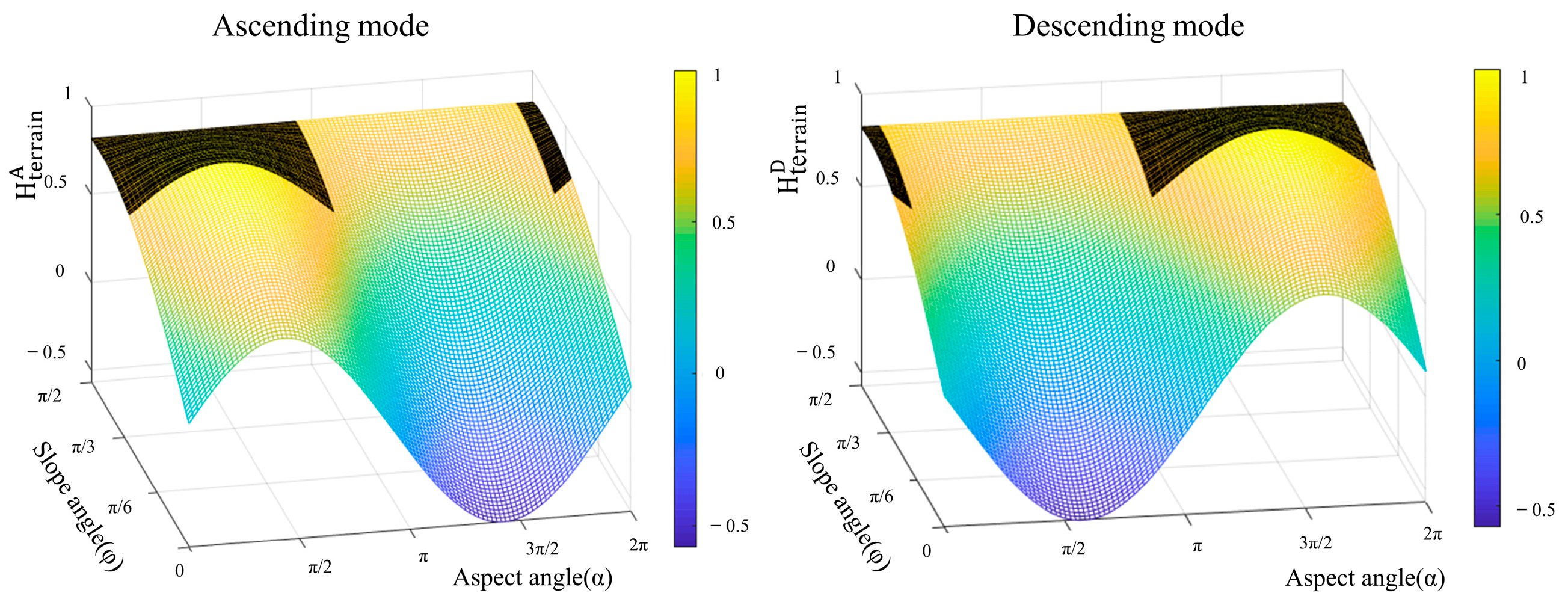
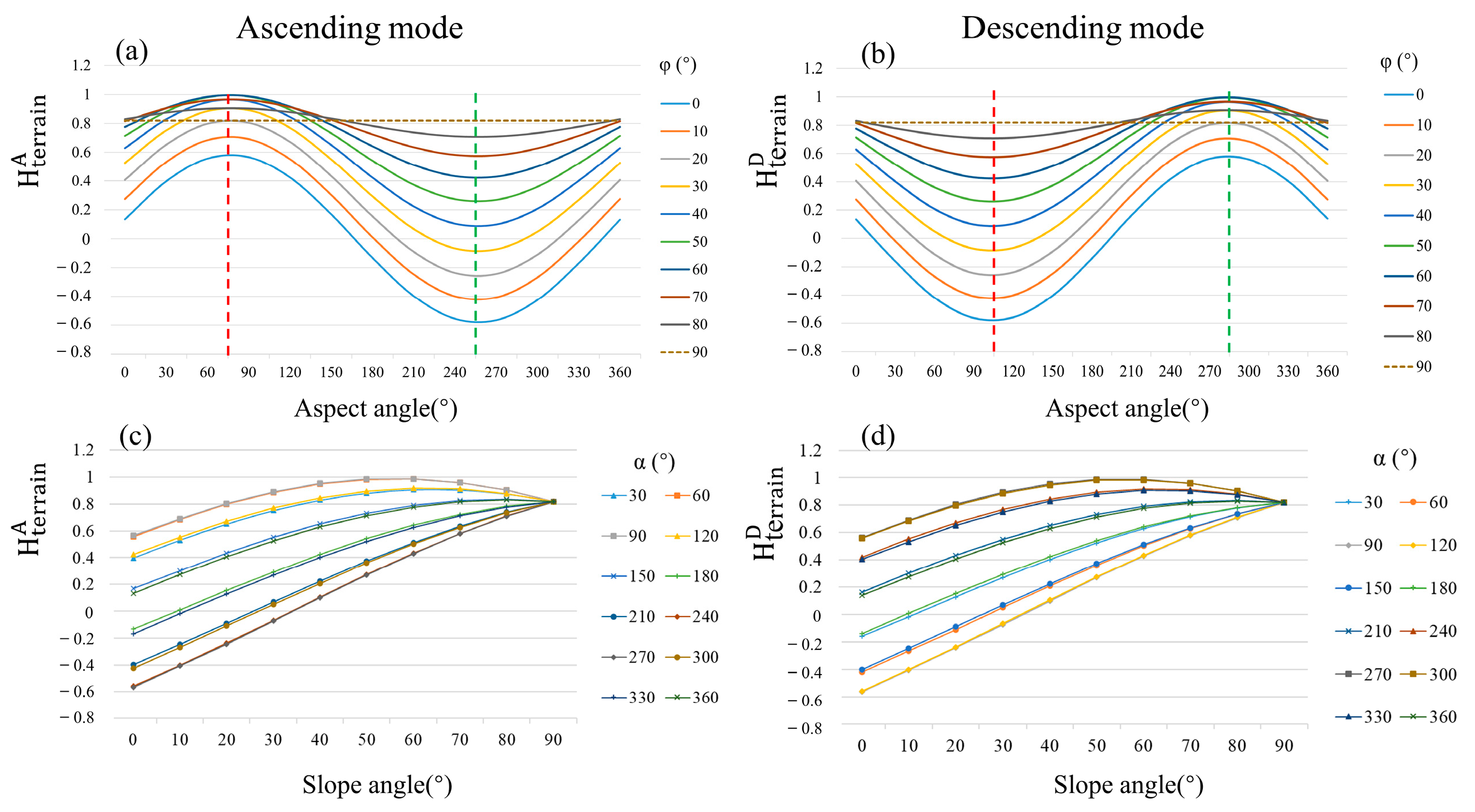
3.3. Slope Angle and Aspect Angle Dependences of Terrain Sensitivity Index (H_terrain)

To describe the slope angle and aspect angle dependences of the terrain sensitivity index intuitively, we simplified Equations (10) and (11) by introducing typical parameters of ascending and descending Sentinel-1 satellites. Generally, the average value of the incident angle for Sentinel-1 satellites is 35°, and the average values of the heading angle for ascending and descending Sentinel-1 orbits are –13.5° and 166.5°, respectively. By substituting these values into Equations (10) and (11), we obtained Equations (12) and (13) of the terrain sensitivity index of the Sentinel-1 ascending and descending orbits, which only contain two unknown parameters of the slope and aspect angles. Notably, the slope angle (φ) and aspect angle (α) of any points on the slope can be obtained through high-precision DEM data.

$$H_{terrain}^A=\mathit{cos}\beta =0.819\mathit{sin}\phi +0.558\mathit{cos}\phi \cdot \mathit{sin}\alpha +0.134\mathit{cos}\phi \cdot \mathit{cos}\alpha$$

(12)

$$H_{terrain}^D=\mathit{cos}\beta =0.819\mathit{sin}\phi -0.558\mathit{cos}\phi \cdot \mathit{sin}\alpha +0.134\mathit{cos}\phi \cdot \mathit{cos}\alpha$$

(13)

To analyze the effects of topographic information, we plotted three-dimensional images of the terrain sensitivity index (H_terrain) of the Sentinel-1 satellite for all possible scenarios in the ascending and descending modes. Negative H_terrain values indicate that the direction of slope displacement is opposite that of satellite LOS. The higher the absolute value of H_terrain, the higher the monitoring sensitivity and probability of monitoring landslide displacement using Sentinel-1 data. When the slope was parallel to the LOS, the terrain sensitivity index was approximately 1. Additionally, it is important to consider unmeasurable problems caused by radar shadowing. In the ascending mode, when the aspect angle is within the range of α $\in$ (0°, 166.5°) $\cup$ (346.5°, 360°) and the slope angle is φ > 55°, radar shadowing will occur, which makes the observation results unusable. Similarly, in the descending mode, when the aspect angle is within the range of α $\in$ (0°, 13.5°) $\cup$ (193.5°, 360°) and the slope angle is φ > 55°, the radar shadowing phenomenon also emerges. The black-shaded portion in Figure 5 shows the values of H_terrain corresponding to the radar shadowing.

Figure 6 shows the change of H_terrain caused by the slope and aspect angles for the ascending and descending orbit modes, respectively. Figure 6a shows the α-H_terrain curves for different slope angles (φ) in ascending mode. The H_terrain of different slope angles reached its maximum when the slope angle (α) was 75° (red dashed line), which indicated that the projection of slope displacement in the LOS direction reached its maximum. If H_terrain = 1, the slope displacement direction coincided with the LOS direction; thus, we could obtain the best sensitivity and result using time-series InSAR. Notably, only the slope angle (φ) was 60°, and the best observation condition of H_terrain = 1 was satisfied. As the aspect angle (α) increased, the curve decreased to lower values, and when the aspect angle (α) was 255° (green dashed line), the H_terrain of different slope angles reached its minimum, and the H_terrain corresponding to the four curves from 0° to 30° were negative values, which indicated that the direction of the slope displacement was back to the sensor, and the active layover occurred. Similar regularity for the descending mode is shown in Figure 6b.

Figure 6c shows the φ-H_terrain curves for different aspect angles (α) in the ascending mode. As the slope angle (φ) increased, H_terrain gradually increased and approached a constant of 0.81 for different aspect angles (α). The curves with 75° and 255° as the symmetry axes showed approximately the same trajectory. Notably, when the slope angle was 0°, the direction of displacement was horizontal, that is, the aspect angle was the same as the displacement direction. When the slope angle was 90°, the direction of displacement was vertical; in this case, the value of H_terrain was 0.81, so the application of Sentinel-1 data to monitor the vertical displacement of the plane had a high sensitivity, which explains why the application of different orbital Sentinel data makes it very easy to monitor the vertical displacements generated by various horizontal surfaces. A similar regularity for the descending mode is shown in Figure 6d, with symmetry axes of 105° and 285°.

4. Results and Analysis

4.1. Case Study of the Qidashan Open-Pit Mine Landslide

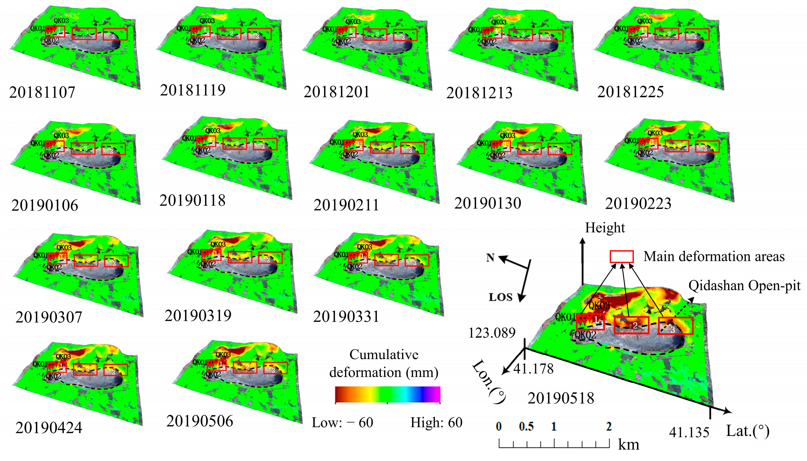
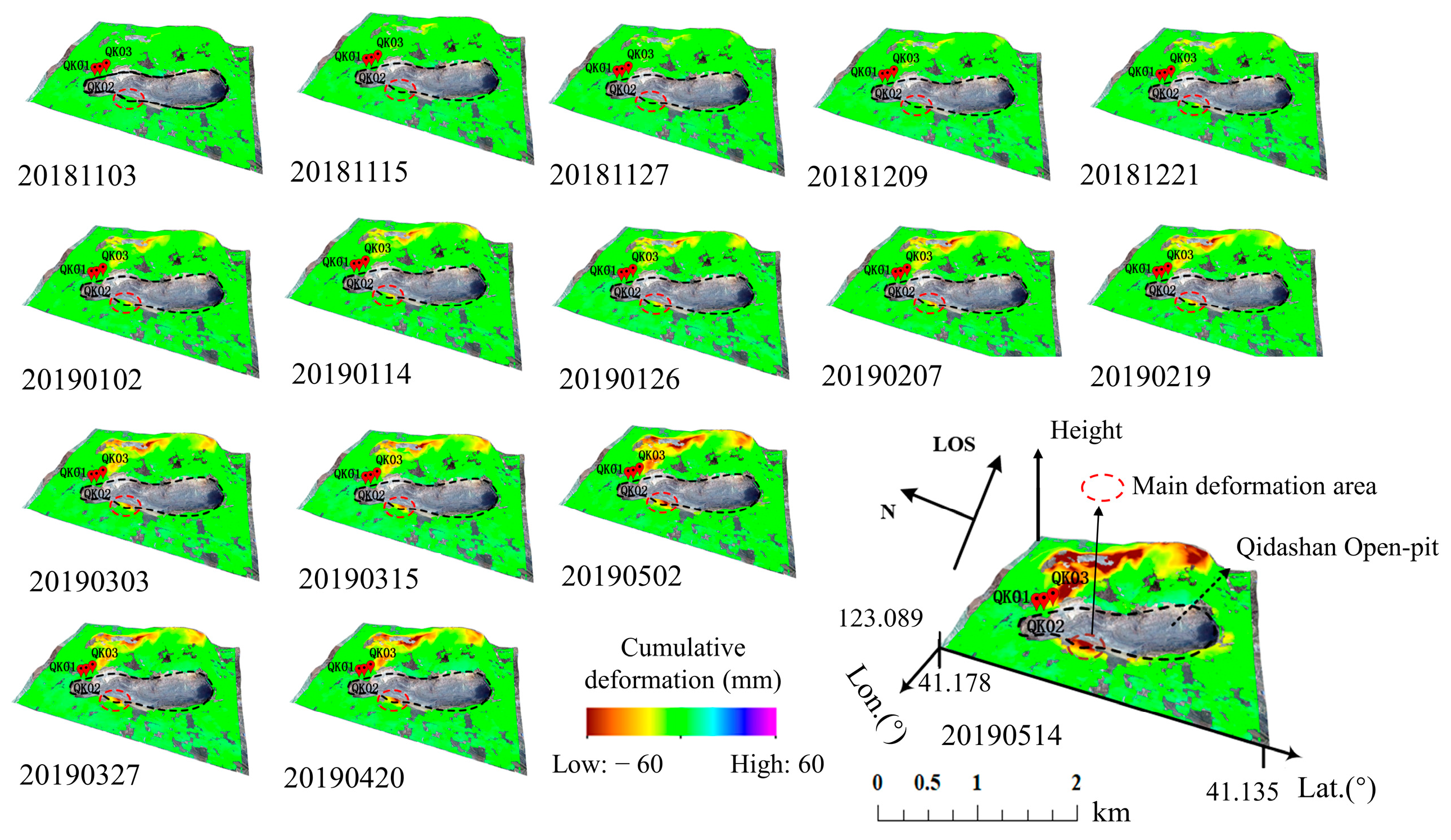
4.1.1. Deformation Monitoring Results of Qidashan Open-Pit Mine Slope Derived from SBAS-InSAR

Based on the spatial baseline threshold of 1.5%, which is relative to the maximum spatial baseline, and the time baseline threshold of 72 d, 69 and 63 image pairs were selected for the ascending and descending orbit data, respectively. The wide coverage of Sentinel-1 IW data was achieved by employing the terrain observation by the progressive scans (TOPS) acquisition mode; however, the non-stationarity of the squint angle during this TOPS acquisition produced a linear variation in the Doppler centroid frequency of the SAR data, resulting in the interferometric processing of the TOPS data to require stringent azimuth registration accuracy (0.001 of the pixel spacing). Therefore, the precise orbit of the Sentinel-1 satellite was used for initial registration, and then the enhanced spectral diversity (ESD) algorithm was used to eliminate the residual geometric offsets of different bursts after the initial registration to obtain the required fine azimuth co-registration accuracy.

Subsequently, we used the Goldstein method to perform interferogram filtering and applied the minimum cost flow (MCF) method to unwrap the phases. The GCP was then used as the stable reference point for orbit refinement and reflattening. The constant residual phase and phase ramp were corrected using GCPs. Finally, we calculated the deformation rate and time-series displacements using the singular value decomposition (SVD) method by removing the influence of the residual DEM error, atmospheric noise, and orbit errors through high-pass filtering in the time domain and low-pass filtering in the frequency domain [40].

The LOS cumulative displacements and deformation rates of the descending and ascending orbits in the Qidashan open-pit mine during the study period are shown in Figure 7, Figure 8 and Figure 9, respectively. As shown in Figure 7, there are three local areas with clear deformation characteristics east of the mine, represented by three solid red rectangles, and the maximum deformation rates in these three areas were −78.1, −56.65, and −117 mm/year, respectively. The negative values are far from the satellite, and the positive values are close to the satellite. Figure 8 shows the deformation monitoring results from the ascending orbit data, which show that there is a clear deformation area west of the mine, represented by the dashed red circle, with a maximum deformation rate of −69 mm/year.

Figure 9 shows the deformation rate of descending and ascending orbits in the study area. The annual average deformation rates monitored by InSAR at three GNSS monitoring stations were −7.7, −20.5, and −47.6 mm/year in descending orbits, while they were −13.2, −34.4, and −105.5 mm/year in ascending orbits. By comparing the LOS deformation rate results from the ascending and descending orbits, a difference between the deformation region monitored by the ascending and descending orbit data is evident, which is consistent with the cumulative deformation results. Next, we quantitatively evaluated the deformation monitoring results of the ascending and descending orbits using theoretical and practical sensitivity indices.

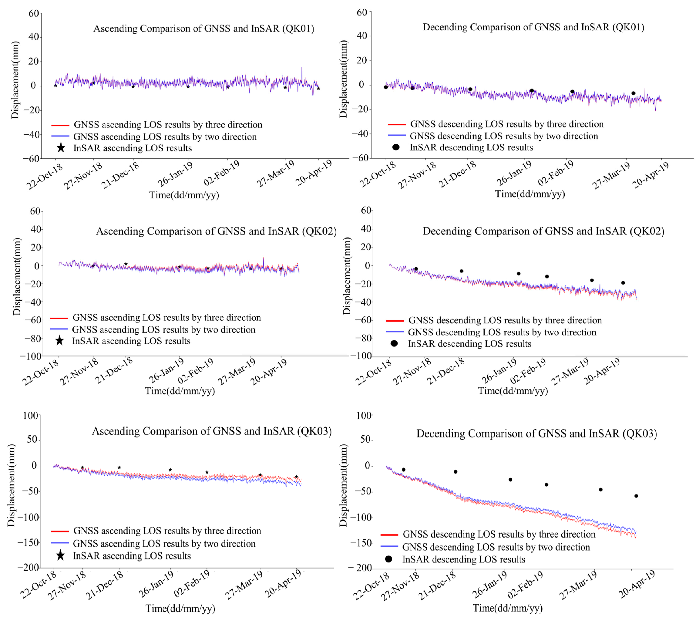
4.1.2. Quantitative Evaluation of InSAR Results from Qidashan Open-Pit Using Theoretical and Practical Sensitivity Indices

First, the projection of slope slip in the LOS direction was calculated by substituting GNSS three-dimensional observation data and satellite geometric parameters of ascending and descending orbits, represented by the red line in Figure 10. Assuming that the slip magnitude in the north–south direction of the slope was 0, only the two-dimensional data in the east–west and up–down directions were used to obtain the projection magnitude of the slope sliding deformation in the LOS direction, represented by the blue line in Figure 10. The results of Figure 10 show that regardless of whether in ascending or descending orbits, the results of LOS projection deformation calculated by three- and two-dimensional deformation information are quite close, which indicates that the influence of north–south deformation on the monitoring results of LOS projection deformation obtained by the Sentinel-1 satellite is small in this case, accounting for only 12% and 13% for ascending and descending orbits, respectively.

We compared the LOS deformation derived from GNSS for ascending and descending modes, represented by the red line in Figure 10, with the LOS deformation obtained from SBAS-InSAR, represented by the black stars and points for ascending and descending in Figure 10, respectively. According to Equation (5), the east–west deformation is the main factor affecting the calculation results of the LOS deformation; therefore, considering the different levels of the east–west deformation magnitude, GNSS monitoring stations with trivial east–west sliding magnitudes (i.e., approximately 10 mm/year), such as the QK01 monitoring station (the up–down, east–west, and north–south deformations were −8.9, −10.4, and −2.5 mm, respectively), the LOS deformation results obtained by SBAS-InSAR matched well with the projection value of the practical sliding magnitude in the LOS direction under both ascending orbit and descending modes. The results from the QK02 monitoring station (the up–down, east–west, and north–south deformation are −26.4, −25.1, and −13.4 mm, respectively), which had a slightly larger deformation magnitude (approximately 30 mm/year) in the east–west direction, were consistent under an ascending orbit mode but deviated slightly between them under a descending orbit mode. When the east–west deformation had a considerable magnitude (approximately 90 mm/year), such as at the QK03 monitoring station (the up–down, east–west, and north–south deformations were −96.9, −86.2, and −60.9 mm, respectively), it only deviated slightly in the ascending orbit mode, but it deviated considerably in the descending orbit mode. However, northeast of the Qidashan open-pit mine slope, the conformity was reasonable under an ascending orbit due to the sharp reduction in the post-projection deformation caused by the projection transform coefficients of the ascending orbit, which made the LOS deformation of the ascending orbit obtained by SBAS-InSAR be only 20% of the practical up–down and east–west deformations. Given a descending orbit, the deviation between them increased gradually with the increase in deformation, but compared with the monitoring results of the ascending orbit, the monitoring results of the descending orbit were more consistent with the practical landslide situation, and the LOS deformation of the descending orbit was approximately 50–70% of the practical up–down and east–west deformations.

Considering the differences in slope sliding directions of different open-pit mines, we used the practical sliding deformation of the open-pit mine as the benchmark parameter for quantitative evaluation of the reliability of landslides monitored by time-series InSAR. The practical sliding of an open-pit mine along the slope direction was calculated using the three-dimensional GNSS deformation results. Combined with the slope deformation vector and satellite imaging geometry, we defined theoretical and practical sensitivity indices for InSAR slope monitoring to quantitatively evaluate the reliability of time-series InSAR in the application of open-pit mine landslide monitoring.

Table 3. GNSS and InSAR displacements and the theoretical and practical indices for slope monitoring sensitivity.

GNSS Site	Method	Three-Dimensional Sliding Magnitude (mm)			LOS Sliding Magnitude (mm)		Slope Slip (mm)	${\mathit{T}}_{\mathit{GNSS}}^{\mathit{A}}$ (%)	${\mathit{P}}_{\mathbf{GNSS}}^{\mathit{A}}$ (%)	${\mathit{T}}_{\mathbf{GNSS}}^{\mathit{D}}$ (%)	${\mathit{P}}_{\mathbf{GNSS}}^{\mathit{D}}$ (%)
		U	E	N	Ascending	Descending
QK01	GNSS	−8.9	−10.4	−2.5	−1.5	−13.5	−13.1	11.5	16.0	103.0	43.5
	InSAR				−2.1	−5.7
QK02	GNSS	−26.4	−25.1	−13.4	−6.7	−37.5	−36.2	18.5	17.4	103.6	47.0
	InSAR				−6.3	−17
QK03	GNSS	−96.9	−86.2	−60.9	−26.2	−136.0	−139.9	18.7	14.2	97.2	35.7
	InSAR				−19.9	−50

shows the theoretical and practical sensitivity indices of slope monitoring calculated using Equations (7) and (8), the three-dimensional slip obtained by GNSS monitoring, and the LOS slip obtained by InSAR monitoring. The calculation results of the theoretical sensitivity index of slope monitoring showed that the $T_{\mathit{GNSS}}^D$ of the descending orbit (average ~ 96%) was significantly better than that of the ascending orbit (average ~ 15%); therefore, the monitoring results of the descending orbit were more reliable than those of the ascending orbit in this study area. Furthermore, the practical InSAR LOS deformation monitoring results were used to calculate the practical sensitivity index of slope monitoring, and the $P_{\mathit{GNSS}}^D$ of the descending orbit (average ~ 40%) was significantly better than that of the ascending orbit (average ~ 15%), which is consistent with the theoretical calculation results. Even with the large-angle sliding of high and steep slopes in the open-pit mine, the monitoring results of the descending orbit can obtain 40% of the slope slip. Generally, when the measurement error meets specific requirements, the theoretical sensitivity indices were larger than the practical sensitivity indices in ascending and descending orbits, indicating that it is difficult to achieve theoretical monitoring accuracy with practical InSAR monitoring because of the comprehensive influence of various errors. Practically, the greater the slope indices (including theoretical and practical sensitivity indices), the higher the reliability of the monitoring results, which has more significance for the identification and monitoring of open-pit mine landslides and can be used as reference data for landslide monitoring and early warning in local regions.

4.1.3. Influence of Topographical Factors on Time-Series InSAR Monitoring Results from Different Orbit Datasets

In the Qidashan open-pit mine case, the point cloud data obtained by LiDAR scanning were used to generate a high-precision DEM of the open-pit mine (Figure 1c), which was used to calculate the accurate slope and aspect angles of the three GNSS monitoring points in the landslide area, as shown in

Table 4. The landslide angle, slope, aspect value and H_terrain of the GNSS station.

GNSS Site	Landslide Angle (°)	Slope (°)	Aspect (°)	Hterrain
				Ascending	Descending
QK01	50.13	53.25	234.9	0.46	0.86
QK02	47.14	41.37	213.3	0.47	0.62
QK03	47.44	53.33	225.6	0.53	0.79

. The slope gradients of the three GNSS stations were greater than 40°, which were in landslide sensitive areas, and the slope and aspect angles were between 202.5° and 337.5°; therefore, the landslide direction of the slope was southwest.

Based on the GNSS monitoring results in the north–south, east–west, and up–down directions, the landslide angles of the three GNSS monitoring stations were calculated. The resulting practical sliding angles and slopes of the three stations were relatively close. In the slope monitoring practice of the Fushunxi [38] and Anqian Yabaling open-pit mines [41] among other large open-pit mines, we found that the landslide angles and gradients of high and steep open-pit mines were highly consistent. Therefore, for high and steep open-pit mines, when there was no or missing GNSS observation data in the study area, we calculated the terrain sensitivity index using Equations (12) and (13) from the slope and aspect angles obtained from the high-precision DEM data. Here, we considered QK01, QK02, and QK03 as examples. The theoretical sensitivity indices of the ascending and descending orbit of the QK01 station were 10.5% and 97.1%, respectively, while those of the QK02 station were 17.2% and 96.8%, respectively, and those of the QK03 station were 18.3% and 95.0%, respectively, as shown in Table 4. The terrain sensitivity index of H_terrain of the ascending and descending orbit modes of the QK01 station were 0.46 and 0.86, respectively, while those of the QK02 station were 0.47 and 0.62, respectively, and those of the QK03 station were 0.53 and 0.79, respectively, as shown in Table 4. The H_terrain of the descending orbit was greater than that of the ascending orbit at all three GNSS stations; therefore, the proposed method can also quantitatively evaluate the reliability of InSAR monitoring results under different orbit conditions when there is an absence of or missing GNSS observation data.

Affected by the complex fluctuation terrain of open-pit mine, time-series InSAR is considerably affected by the slope gradient in the surface deformation monitoring of the open-pit mine. When the slope angle is large, geometric distortion (shadow and layover) occurs in the SAR image [42]. When the radar was in an ascending orbit, the topographic slope angle was greater than the radar incident angle $\left(\alpha >\theta \right)$ and the layover was formed; however, when the radar was in descending orbit, the layover area was formed when the angle of the topographic slope on the back slope of the radar incident was greater than the residual angle of the radar incident angle $\left(\alpha >\pi /2-\theta \right)$.

Considering the practical situation of the QK01 monitoring station as an example, during an ascending orbit, the sliding direction was the same as the radar LOS. According to Table 3, the slope angle of this station was greater than the radar incidence angle; therefore, it is difficult for InSAR to obtain useful phase information in the layover area. Combined with the calculation results of Equation (6), the monitoring magnitude of the InSAR LOS under an ascending orbit was found to be small; therefore, we determined that layover occurred during SAR imaging. In contrast, during a descending orbit, the sliding direction is opposite that of the radar LOS. As shown in Table 4, the angle of the terrain slope of the station on the back slope of the radar incidence was less than the residual angle of the radar incidence angle; therefore, we determined that no layover area is formed during SAR imaging (i.e., QK02 and QK03 were similar to QK01).

Therefore, when monitoring the landslide in the surrounding area of the three GNSS stations of the Qidashan open-pit mine, the layover phenomenon was not conducive to landslide monitoring by the InSAR technique, which affected the accuracy of landslide identification and monitoring; however, no observation error was caused by the descending orbit images during the imaging process of the study area. According to the calculated values of ascending and descending orbits at three GNSS monitoring stations, the monitoring magnitude of the ascending orbit was smaller than that of the descending orbit; therefore, estimating the landslide deformation by using the monitoring results of the descending orbit was more accurate than using the ascending orbit when applying InSAR to identify and monitor landslides in the study area.

4.2. Case Study of the Yabaling Open-Pit Mine Landslide

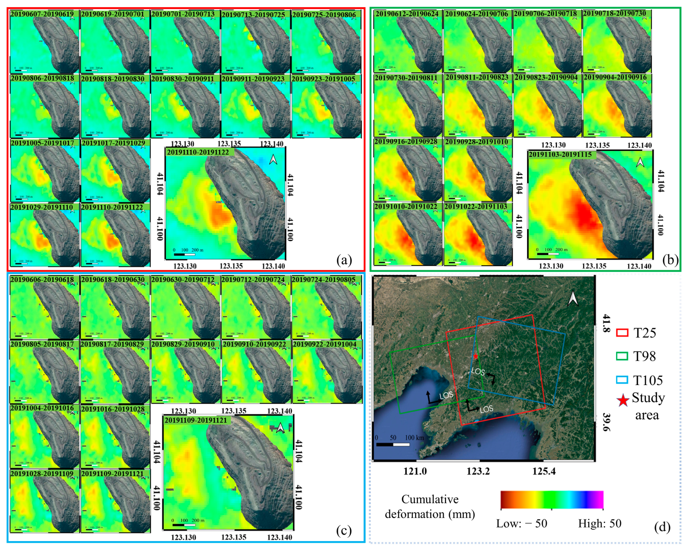
4.2.1. Deformation Monitoring Results of Yabaling Open-Pit Mine Slope Derived from SBAS InSAR

We processed the datasets from three different orbits using the SBAS-InSAR technique and obtained three results of LOS time-series deformation in the study area, as shown in Figure 11. Figure 11a,b shows the monitoring results of the ascending dataset for the T25 and T98 orbits, respectively. Figure 11c shows the monitoring results of the descending dataset for the T105 orbit. Negative values (red) indicate ground motion away from the satellite, while positive values (blue) indicate ground motion toward the satellite. The InSAR monitoring results obtained from the two ascending orbit datasets indicated that there was an anomalous deformation on the southwest slope of the Yabaling open-pit mine (where the landslide occurred); however, the deformation information was insensitive to the monitoring results obtained from the descending orbit dataset.

4.2.2. Evaluation of Monitoring Results for Three Different Orbital Datasets Using H_terrain

For the three different orbital datasets, only the two ascending datasets obtained the effective deformation of the landslide area before the landslide, whereas the descending dataset had low sensitivity to the deformation region and failed to effectively monitor the deformation information of the landslide area. We selected the location with the largest deformation, which is indicated by the red dot on Figure 2, as the study point, and according to the global 12.5 m DEM data provided by the ALOS satellite, the slope angle of this point was 39.95° and the aspect angle was 49.82°. Bringing these two parameter values into Equations (12) and (13), we calculated the values of H_terrain under the two ascending (T25 and T98) and the descending orbit (T105) datasets as 0.90, 0.93, and 0.07, respectively, and it is clear that the sensitivity of the descending orbit dataset to the deformation of this study area was very low and could not be monitored. Therefore, if the H_terrain value could be calculated using known DEM data before InSAR data processing, a dataset with a high-monitoring sensitivity could be selected using a priori knowledge. For this case, only datasets with high H_terrain values were selected as the data source, which greatly improved the efficiency of landslide monitoring using InSAR.

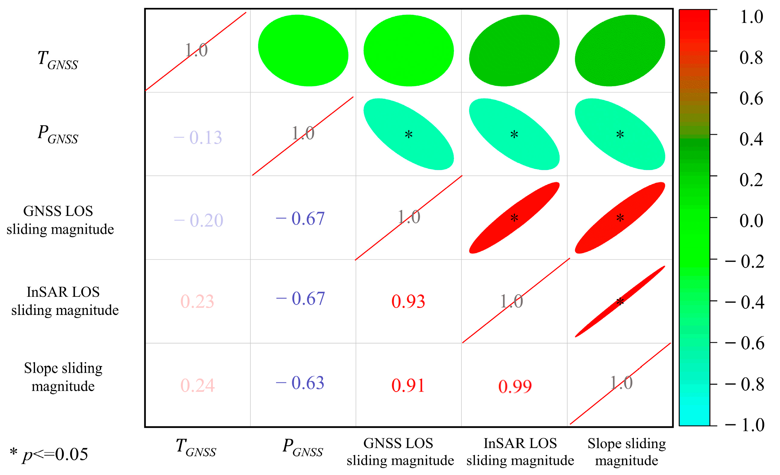
4.3. Statistical Analysis of the Sensitivity Evaluation Indices

Different landslide events have shown that the types, sizes, geological conditions, mechanical parameters, and trigger factors of landslides differ. To verify whether the indices proposed in this study are widely applicable, we performed a statistical study on the theoretical, practical, and terrain sensitivity indices. Although landslides are complex geological disasters, we demonstrate that it is possible to quantitatively describe the credibility of landslide monitoring for high and steep slopes using this time-series InSAR technique.

4.3.1. Statistical Analysis of Landslide Cases with Both GNSS and InSAR Monitoring Data

To statistically prove the generalizability of the theoretical and practical sensitivity indices, we needed landslide cases with both GNSS and InSAR monitoring data. However, we reviewed over 300 papers on InSAR landslide monitoring, and only four typical landslide cases were found with both GNSS and InSAR monitoring data to perform statistical analysis. We calculated the theoretical and practical sensitivity indices of 15 GNSS monitoring stations for these landslide events (

Table A1. Landslide events with both public GNSS and InSAR data.

No.	Authors	Landslide Name	Landslide Territory	Methodology	Study Time	Number of Images	Satellite Mission
Case 1	[43]	Patigno landslide	Northern Apennines, Italy	PS-InSAR	March 2015–May 2019	200	Sentinel-1
Case 2	[44]	Bosmatto landslide	Northwestern Alps, Italy	SqueeSAR	October 2014–February 2018	130	Sentinel-1
Case 3	[45]	potential landslide	Shananxi Provice, China	CR-InSAR	April 2011–August 2011	4	TerraSAR
Case 4	[46]	Sirobagarh landslide	Uttarakhand, India	MT-InSAR	November 2015–August 2017	10	Sentinel-1

in Appendix A).

Table 5. Theoretical and practical sensitivity indices of different landslides.

No.	Authors	Satellite Mission	Area of Study	Methodology	Study Time	Number of Stations	Typical Station	TGNSS	PGNSS
Case 1	[43]	Sentinel-1	Northern Apennines	PS-InSAR	March 2015–May 2019	1	PATG	76.6%	54.7%
Case 2	[44]	Sentinel-1	Bosmatto	SqueeSAR	April 2014–April 2016	4	A-06	92.8%	68.3%
Case 3	[45]	TerraSAR	Shananxi Province	CR-InSAR	April 2011–August 2011	6	DJ-08	88.0%	64.4%
Case 4	[46]	Sentinel-1	Uttarakhand	MT-InSAR	November 2015–August 2017	4	GPS4	99.8%	135.9%

shows the calculation results of the theoretical and practical sensitivity indices of representative GNSS monitoring sites in each landslide case (the results for all GNSS sites are shown in

Table A2. Theoretical and practical sensitivity index of different landslides of four cases.

No.	Incidence Angle (°)	Azimuth Angle (°)	GNSS Deformation (mm)/Rate (mm/Year)			InSAR LOS Deformation (mm)/Rate (mm/Year)	Slope Slip (mm)/Rate (mm/Year)	Station	TGNSS (%)	PGNSS (%)
			VN	VE	VU
Case 1	40.31	−80.73	−33.5	12.2	−3.2	9.0	16.5	PATG	76.6%	54.7%
Case 2	43.12	280.49	−4.3		−7.4	−6.1	−8.5	A-05	97.4%	71.6%
			−18.8		−8.5	−13.9	−20.4	A-06	92.8%	68.3%
			−33.2		−28.8	−35.8	−43.6	M-05	99.7%	82.2%
			−26.3		−14.9	−21.1	−29.9	M-06	95.8%	70.8%
Case 3	35.00	−7.44	−2	−3	−6	−0.8	−6.6	DJ-02	46.3%	12.1%
			−3	0	−7	−3.5	−5.6	DJ-04	97.6%	62.0%
			0	−1	−2	−2.9	−1.9	DJ-05	54.9%	148.8%
			−4	−2	−10	−11.7	−10.1	DJ-06	67.2%	116.3%
			−3	3	−15	−9.1	−13.9	DJ-07	98.6%	65.2%
			4	−6	−34	−18.1	−28.1	DJ-08	88.0%	64.4%
Case 4	35.00	−13.5	14.2	3.2	−219.0	−334.1	−220.1	GPS1	83.2%	156.7%
			36.1	19.4	−220.9	−575.6	−449.8	GPS2	43.7%	128.8%
			264.0	47.0	−296.2	−407.6	−304.8	GPS4	99.8%	135.9%
			12.7	12.9	252.1	−252.7	−265.2	GPS6	81.2%	140.7%

in Appendix A). The statistical results show that all the theoretical sensitivity indices showed a strong correlation with the practical sensitivity index; that is, the larger the theoretical sensitivity index, the larger the practical sensitivity index, indicating higher feasibility of using time-series InSAR for landslide monitoring. Furthermore, the theoretical and practical sensitivity indices were only applicable to the Sentinel-1 satellite data used in this study and TerraSAR satellite data.

According to the definitions of the theoretical and practical sensitivity indices, the theoretical sensitivity index should be larger than the practical sensitivity index; however, we found that the practical sensitivity index of some monitoring stations was larger than the respective theoretical sensitivity index, such as in monitoring points DJ05 and DJ06 from Case 3 (Table A2 in Appendix A) and all four monitoring points from Case 4. Under the assumption that the GNSS monitoring data were relatively accurate, this is caused by the InSAR measurement errors; for example, the displacement along the north–south direction and the low-precision DEM data. This indicates that the theoretical and practical sensitivity indices can be jointly used to assess the accuracy of the InSAR measurements.

We further performed a statistical analysis for the correlations between the five variables of the 15 GNSS monitoring stations from these studies: T_GNSS, P_GNSS, slope sliding magnitude, InSAR, and GNSS sliding magnitude along the LOS. As shown in Figure 12, we calculated the Pearson correlation coefficients between each two variables, and the * in the figure indicates a significant correlation between these two variables (p < 0.05). The correlation between T_GNSS and the other four variables was poor, while the other variables were significantly correlated with each other. This was also caused by a measurement error of the InSAR itself; therefore, we can directly assess the feasibility and accuracy of InSAR monitoring according to the T_GNSS and P_GNSS indices when the deformation values monitored by GNSS were relatively accurate. (1) When T_GNSS was small, the deformation of the monitoring station was not easily monitored by InSAR, and its feasibility was low. (2) When P_GNSS > T_GNSS, there were errors in the InSAR monitoring results, and the reliability of the InSAR monitoring results was low. (3) When T_GNSS > P_GNSS and T_GNSS were sufficiently large, both the T_GNSS and P_GNSS could be utilized to evaluate the sensitivity of time-series InSAR monitoring results.

4.3.2. Statistical Analysis of Landslide Cases Monitored by InSAR without GNSS Data

We found 119 global cases of successful landslide monitoring by applying InSAR [47,48,49,50] and calculated the terrain sensitivity index (H_terrain) of them, and the detailed data of all calculations are shown in

Table A3. Terrain sensitivity index calculation results of landslides along the Jinsha river, China [48].

No.	Landslide Name	Slope Min	Slope Max	Average Slope	Aspect	${\mathit{H}}_{\mathbf{terrain}}^{\mathit{A}}$
1	Dangdi No. 1	28	38	33	60	0.90
2	Dangdi No. 2	26	44	35	16	0.70
3	Dangdi No. 3	23	40	31.5	51	0.86
4	Ningkang	10	42	26	118	0.74
5	Redangong	22	38	30	27	0.73
6	Aiguo	18	44	31	113	0.81
7	Aibai	20	39	29.5	92	0.88
8	Gaina	16	39	27.5	30	0.72
9	Woda	16	40	28	19	0.65
10	Moga	27	42	34.5	117	0.82
11	Tange	22	45	33.5	67	0.92
12	Duolai	18	36	27	108	0.80
13	Shadingmai	15	40	27.5	117	0.76
14	Adong	19	39	29	51	0.84
15	Xiaomojiu	21	42	31.5	50	0.86
16	Xiongba No. 1	15	46	30.5	23	0.71
17	Xiongba No. 2	15	51	33	133	0.71
18	Xiongba No. 3	20	40	30	215	0.05
19	Semai	10	40	25	273	−0.13
20	Wadui	16	40	28	107	0.81
21	Gongba	15	39	27	112	0.78
22	Maiba No. 1	24	42	33	243	−0.01
23	Maiba No. 2	34	46	40	222	0.18
24	Shangquesuo	18	37	27.5	131	0.67
25	Shangde	16	37	26.5	28	0.70
26	Decun	20	40	30	112	0.80
27	Suoxue	20	38	29	346	0.40
28	Chutigang No. 1	19	44	31.5	162	0.47
29	Chutigang No. 2	24	48	36	20	0.74
30	Caodigong	20	49	34.5	47	0.87
31	Suoduxi	11	30	20.5	124	0.64
32	Sarongxue	24	45	34.5	134	0.72
33	Nanagong	10	40	25	44	0.78
34	Diwu	10	30	20	217	−0.12
35	Namu	16	35	25.5	111	0.77
36	Linong	15	64	39.5	95	0.94
37	Dagu	18	56	37	142	0.68
38	Qinbei	10	16	13	107	0.67
39	Dongan No. 1	10	33	21.5	12	0.53
40	Dongan No. 2	12	33	22.5	21	0.61
41	Hongguang	21	36	28.5	64	0.88
42	Fangjiapo	27	43	35	128	0.76
43	Nawudu	16	45	30.5	11	0.62
44	Shangyingwo	16	51	33.5	113	0.84
45	Yazishou	15	36	25.5	190	0.15
46	Xincun	15	45	30	25	0.72
47	Zhongwushan	10	55	32.5	78	0.92
48	Xiaoshuijing	24	44	34	185	0.31
49	Jinpingzi	10	40	25	141	0.57
50	Dadi	10	51	30.5	171	0.38
51	Yangpengzi	34	51	42.5	144	0.72
52	Luogazhi	13	47	30	104	0.85
53	Yeniuping	29	45	37	178	0.40
54	Hejialiangzi	14	30	22	230	−0.17
55	Damuchun	14	40	27	209	0.03
56	Dashannao	17	51	34	178	0.36
57	Yezhutang	11	41	26	61	0.86
58	Huangtian	13	28	20.5	62	0.80
59	Jiashantian	14	34	24	121	0.70
60	Zengjiawanzi	14	46	30	308	0.10
61	Yizi	10	22	16	290	−0.23
62	Ximaxi	10	50	30	98	0.87
63	Yanwan	20	42	31	77	0.91
64	Ribucu	29	42	35.5	25	0.77
65	Shangshawa	10	38	24	145	0.53
66	Nongle	10	60	35	106	0.88
67	Xianglushan	13	31	22	150	0.46
68	Wufutang	10	30	20	40	0.719
69	Guanghui	10	23	16.5	216	−0.19

,

Table A4. Terrain sensitivity index calculation results of landslides in Gongjue county, Tibet, China [49].

No.	Landslide Name	Slope Min	Slope Max	Average Slope	Aspect	${\mathit{H}}_{\mathbf{terrain}}^{\mathit{A}}$	${\mathit{H}}_{\mathbf{terrain}}^{\mathit{D}}$
70	Laduoting	22	43	32.5	342	0.38	0.47
71	Shadong	15	38	26.5	75	0.87	−0.29
72	Sela	15	51	33	125	0.78	−0.02
73	Geguo	18	42	30	215		0.78
74	Majue	20	38	29	70	0.89	−0.24
75	Guoba	14	36	25	75	0.86	−0.32
76	Gongba	10	35	22.5	91	0.83	−0.35
77	Shangquesuo	20	40	30	140	0.66	0.06
78	Shangde No. 1	15	34	24.5	60	0.83
79	Shangde No. 2	15	32	23.5	45	0.76	−0.23
80	Decun	14	34	24	350	0.34	0.29
81	Suoxue No. 1	18	44	31	90	0.90	−0.21
82	Suoxue No. 2	22	38	30	349		0.37

,

Table A5. Terrain sensitivity index calculation results of landslides in Baihetan reservoir, China [47].

No.	Landslide Name	Slope Min	Slope Max	Average Slope	Aspect	${\mathit{H}}_{\mathbf{terrain}}^{\mathit{A}}$	${\mathit{H}}_{\mathbf{terrain}}^{\mathit{D}}$
83	H01	23	30	26.5	80	0.91
84	H02	25	45	35	5	0.61	0.30
85	H03	22	34	28	48	0.85
86	H04-2	28	46	37	340	0.41	0.54
87	H05	34	54	44	162	0.60
88	H07	30	40	35	88	0.95
89	H08	28	46	37	173	0.41
90	H09	40	56	48	38	0.90
91	H11	28	40	34	73	0.95
92	H12	40	58	49	320	0.40	0.78
93	H13	40	60	50	22	0.83	0.37
94	H14	16	40	28	318	0.10	0.64
95	H15-2	40	50	45	323	0.38
96	H16	15	50	32.5	258		0.94
97	H17	25	46	35.5	208		0.78
98	H18	16	54	35	270		0.94

and

Table A6. Terrain sensitivity index calculation results of landslides in Danba, Sichuan, China [50].

N0.	Slope Min	Slope Max	Average Slope	Aspect	${\mathit{H}}_{\mathbf{terrain}}^{\mathit{A}}$	${\mathit{H}}_{\mathbf{terrain}}^{\mathit{D}}$
99	15	25	20	105	0.80
100	15	25	20	100	0.83
101	15	25	20	90	0.87
102	25	40	32.5	130	0.70
103	30	45	37.5	266		0.96
104	20	45	32.5	130	0.70
105	30	45	37.5	177		0.56
106	20	40	30	200		0.68
107	15	30	22.5	50	0.87
108	20	35	27.5	236		0.87
109	15	20	17.5	227		0.75
110	20	35	27.5	200		0.66
111	15	30	22.5	310		0.64
112	20	25	22.5	290		0.77
113	25	30	27.5	260		0.91
114	15	25	20	307		0.64
115	25	30	27.5	280		0.86
116	15	35	25	300		0.74
117	25	35	30	60	0.95
118	20	25	22.5	40	0.82
119	20	40	30	130	0.69

in Appendix A. Notably, the calculated H_terrain values were between approximately –1.0 and 1.0, according to which the visibility of a certain region monitored by InSAR could be evaluated: (1) if H_terrain was greater than or equal to sin φ (H_terrain ≥ sin φ), the region has good visibility; (2) if H_terrain was between 0 and sin φ (0 < H_terrain < sin φ), the region has medium visibility and is a foreshortening region; and (3) if H_terrain was less than or equal to 0 (H_terrain ≤ 0), the area had poor visibility and was an active layover layer.

As shown in Figure 13, our statistical results showed that the medium visibility and above areas (classifications (1) and (2) above) accounted for 98% of all landslide cases successfully monitored using InSAR technology, indicating that 119 landslide cases could be determined by calculating the H_terrain value to determine whether they could be monitored using InSAR, and two landslide cases (2%) showed an active layover area with poor visibility but were still monitored by InSAR. This demonstrated the high accuracy of our proposed terrain sensitivity index in satellite visibility analysis (98% of all landslide cases). Thus, the statistical results showed that the visibility of landslides monitored using the SAR dataset can be reasonably assessed by calculating the H_terrain value before InSAR data processing, thereby greatly improving the efficiency of InSAR monitoring.

5. Discussion

SAR satellites usually fly in a polar orbit with a flight path close to a north–south direction, which results in InSAR being insensitive to north–south deformation monitoring. In this study, for the case of a landslide in the Yabaling open-pit mine, we found significant variability in the results monitored by SAR datasets of different orbits for the same study area. For large deformations in the area, no useful deformation information was monitored by the descending dataset, indicating that different orbit datasets have different sensitivities for this study area. To further demonstrate the effectiveness of the proposed terrain sensitivity index H_terrain for studying such a small-scale area in the mining region, as shown in Figure 14, we plotted the distribution of the terrain sensitivity index H_terrain for the Yabaling open-pit mine based on the geometric parameters of three different orbiting satellites and topographic influences (slope and aspect angles), which was used to illustrate the sensitivity of the different orbiting datasets to monitor the sensitivity of the Yabaling open-pit mine.

In Figure 14d–f, the blue region represents H_terrain > sin φ, which is monitored with high sensitivity (good satellite visibility, no layover and foreshortening effect), and the red and light blue regions represent the layover and foreshortening effect, respectively. As the maximum slope angle of the study area was 40° (Slope_max < π/2 − φ), there was no shadow in this area. By comparison, in the deformation area (red ellipse in Figure 14a), the blue (high sensitivity) area of the ascending orbit 2 (T98) dataset was the largest, whereas the descending orbit (T105) dataset was the least, which reasonably explained the variability of the monitoring results (Figure 11) for the three different orbit datasets. Simultaneously, these three maps show the approximate outline location of the mine area with some color mutations. The main reason for this situation is that the spatial resolution and elevation accuracy of the DEM data used is insufficient, that is, the 12.5 m external DEM data provided by the ALOS satellite are still not fine enough for the small-scale area of the mine area. In large-scale areas, this color mutation phenomenon was weaker than in small-scale areas. In the future, we will try to acquire finer DEM data (e.g., up to a 25 cm spatial resolution LiDAR dataset), which will help us further investigate the problem.

To further demonstrate that the index proposed in this study has advantages in small-scale regions, we compared the H_terrain index with the R-index in our study areas, with the results shown in

Table 6. Comparison between R-index and H_terrain for two landslide cases.

Landslides	GNSS Site/ SAR Datasets	Slope (φ)	Aspect (α)	R-Index		Hterrain
				Ascending	Descending	Ascending	Descending
Qidashan open-pit mine	QK01	53.25	234.9	−0.03	−0.27	0.34	0.99
	QK02	41.37	213.3	0.34	0.06	0.25	0.86
	QK03	53.33	225.6	0.09	−0.21	0.38	0.95
Yabaling open-pit mine	Ascending1 (T25)	39.95	49.82	0.81		0.90
	Ascending2 (T98)			0.89		0.93
	Descending (T105)			0.97		0.07

. In the landslide case of the first Qidashan open-pit, the calculated results of the R-index showed a low sensitivity for both the ascending and descending datasets, whereas the calculated results of the H_terrain showed that the sensitivity index of the descending dataset was approximately two to three times higher than that of the ascending dataset, and the descending dataset had a high sensitivity in this region and can monitor significant deformation, which is consistent with the actual situation. In the second case of the landslide at the Yabaling open-pit, we calculated the R-index and H_terrain at the point of the maximum deformation (red dot in Figure 2). The results showed that both indices were good indicators of the high sensitivity of the ascending orbit datasets, with the H_terrain index showing somewhat higher sensitivity; however, for the descending orbit dataset, a significant difference was observed. The calculated R-index indicated that the descending orbit dataset had a high sensitivity in this region, while the calculated H_terrain showed that the descending orbit dataset had a very low sensitivity, in the range of not being monitored. The monitoring results show that the descending orbit dataset failed to monitor the effective deformation information in this region, indicating that the calculated H_terrain results were consistent with the actual deformation results.

Notably, the existing studies on sensitivity indices mainly assess and analyze the visibility of a large study area [20,23], and the sensitivity index H_terrain proposed in this paper has been experimentally and statistically proven to be applicable to assess the feasibility of satellite monitoring in both large and small regions; however, if there are GNSS monitoring stations, the proposed theoretical and practical sensitivity indices can be used for quantitative evaluation. We searched a substantial number of published studies on landslide deformation monitoring, from which we found cases with both GNSS and InSAR monitoring results and analyzed them to verify the proposed theoretical and practical sensitivity indices. The 15 GNSS monitoring stations in the four landslide cases (Table A2 in Appendix A) can prove that our proposed sensitivity index can be used for the quantitative evaluation of the reliability of InSAR monitoring results, but a considerable number of cases are still needed for additional validation in the future, and we hope that more scholars will publicize the GNSS and InSAR datasets used for landslide studies for subsequent studies.

Additionally, we found a case study on landslide monitoring that supports the idea that the terrain sensitivity index proposed in this paper has a better discriminative effect for applications. Some scholars monitored two landslides in Indonesia using the MT-InSAR technique based on ascending and descending orbit datasets [51], but only the pre-landslide deformation information was monitored in the ascending orbit dataset. Based on the R-index calculation method [52], they calculated an R-index of 0.82 and 0.71 for the ascending and descending orbit datasets, respectively, indicating that the deformation information of the study area can be obtained for both the ascending and descending orbit datasets; however, the monitoring results show that no deformation information was monitored in the descending orbit dataset, indicating that the R-index overestimated the monitoring capability of the descending orbit dataset in this area. By applying the terrain sensitivity index proposed in this study, the results show that the H_terrain of the ascending orbit dataset is 0.81, which has high monitoring sensitivity, whereas the H_terrain of the descending orbit dataset is 0.49, which is in the perspective shrinkage range and has poor monitorability (

Table A7. Terrain sensitivity index calculation results of Ciloto landslide [51].

No.	Landslide Name	Average Slope	Aspect Min	Aspect Max	Aspect	${\mathit{H}}_{\mathbf{terrain}}^{\mathit{A}}$	${\mathit{H}}_{\mathbf{terrain}}^{\mathit{D}}$
120	Puncak Pass	60	130	160	135	0.81	0.50

in Appendix A). The sensitivity of the ascending orbit dataset to the study area was approximately twice as high as that of the descending orbit dataset. Therefore, the H_terrain proposed in this study has a better differentiation effect in quantitatively describing the monitoring sensitivity of satellite data.

6. Conclusions

Large open-pit mines are characterized by large and steep slopes and complex terrain. The LOS deformation obtained by the time-series InSAR method has certain limitations in landslide monitoring of open-pit mines. In this study, the reliability and applicability of the InSAR monitoring results of the Qidashan and Yabaling open-pit mines were quantitatively studied. Based on the deformation variables of the landslides along the LOS direction of the open-pit mines and combining the InSAR monitoring results, GNSS monitoring results, high-precision DEM data, and geometric parameters of satellites, evaluation indices of the reliability of the slope displacement results based on time-series InSAR monitoring were proposed, that is, theoretical, practical, and terrain sensitivity indices, for slope monitoring.

When the theoretical and practical sensitivity indices for slope monitoring were significant, it was easier to monitor small-scale landslide deformation, which can be used as a priori knowledge for monitoring landslides in open-pit mines using InSAR technology. In the two experimental cases of this study, the theoretical and practical sensitivity indices of the first Qidashan open-pit mine from the descending orbit dataset were two to three times higher than those of the ascending orbit dataset; therefore, the descending orbit dataset was more suitable for landslide monitoring of the northeast slope of the Qidashan open-pit mine. However, the terrain sensitivity index of the ascending orbit dataset was significantly larger than that of the descending orbit dataset in the second Yabaling open-pit mine. Therefore, the ascending orbit dataset was more suitable for landslide monitoring in the Yabaling open-pit mine.

Numerous landslide examples, that is four landslide cases with GNSS monitoring data and one hundred nineteen landslide cases without GNSS monitoring data, statistically verified that the sensitivity index proposed in this study has universal applicability and can quantitatively evaluate the reliability of InSAR monitoring results of different orbits, which is of great significance for the identification and monitoring of local landslides for high and steep slopes in small regions. Additionally, the calculation method based on the Sentinel-1 sensitivity index proposed in this study can be easily extended to other satellite constellations.

References

1. Chae, B.-G.; Park, H.-J.; Catani, F.; Simoni, A.; Berti, M. Landslide prediction, monitoring and early warning: A concise review of state-of-the-art. Geosci. J. 2017, 21, 1033–1070. [Google Scholar] [CrossRef]
2. Lu, Z.; Kim, J. A Framework for Studying Hydrology-Driven Landslide Hazards in Northwestern US Using Satellite InSAR, Precipitation and Soil Moisture Observations: Early Results and Future Directions. GeoHazards 2021, 2, 17–40. [Google Scholar] [CrossRef]
3. Park, S.; Lim, H.; Tamang, B.; Jin, J.; Lee, S.; Chang, S.; Kim, Y. A Study on the Slope Failure Monitoring of a Model Slope by the Application of a Displacement Sensor. J. Sens. 2019, 2019, 7570517. [Google Scholar] [CrossRef]
4. Carla, T.; Nolesini, T.; Solari, L.; Rivolta, C.; Dei Cas, L.; Casagli, N. Rockfall forecasting and risk management along a major transportation corridor in the Alps through ground-based radar interferometry. Landslides 2019, 16, 1425–1435. [Google Scholar] [CrossRef] [Green Version]
5. Ouyang, C.; Zhao, W.; An, H.; Zhou, S.; Wang, D.; Xu, Q.; Li, W.; Peng, D. Early identification and dynamic processes of ridge-top rockslides: Implications from the Su Village landslide in Suichang County, Zhejiang Province, China. Landslides 2019, 16, 799–813. [Google Scholar] [CrossRef]
6. Uhlemann, S.; Smith, A.; Chambers, J.; Dixon, N.; Dijkstra, T.; Haslam, E.; Meldrum, P.; Merritt, A.; Gunn, D.; Mackay, J. Assessment of ground-based monitoring techniques applied to landslide investigations. Geomorphology 2016, 253, 438–451. [Google Scholar] [CrossRef] [Green Version]
7. Yang, F.; Jiang, Z.; Ren, J.; Lv, J. Monitoring, Prediction, and Evaluation of Mountain Geological Hazards Based on InSAR Technology. Sci. Program. 2022, 2022, 2227049. [Google Scholar] [CrossRef]
8. Zhang, T.; Zhang, W.; Yang, R.; Gao, H.; Cao, D. Analysis of Available Conditions for InSAR Surface Deformation Monitoring in CCS Projects. Energies 2022, 15, 672. [Google Scholar] [CrossRef]
9. Pawluszek-Filipiak, K.; Borkowski, A. Integration of DInSAR and SBAS Techniques to Determine Mining-Related Deformations Using Sentinel-1 Data: The Case Study of Rydutowy Mine in Poland. Remote Sens. 2020, 12, 242. [Google Scholar] [CrossRef] [Green Version]
10. Berardino, P.; Fornaro, G.; Lanari, R.; Sansosti, E. A new algorithm for surface deformation monitoring based on small baseline differential SAR interferograms. IEEE Trans. Geosci. Remote Sens. 2002, 40, 2375–2383. [Google Scholar] [CrossRef] [Green Version]
11. Lanari, R.; Mora, O.; Manunta, M.; Mallorqui, J.J.; Berardino, P.; Sansosti, E. A small-baseline approach for investigating deformations on full-resolution differential SAR interferograms. IEEE Trans. Geosci. Remote Sens. 2004, 42, 1377–1386. [Google Scholar] [CrossRef]
12. Zhang, P.; Guo, Z.; Guo, S.; Xia, J. Land Subsidence Monitoring Method in Regions of Variable Radar Reflection Characteristics by Integrating PS-InSAR and SBAS-InSAR Techniques. Remote Sens. 2022, 14, 3265. [Google Scholar] [CrossRef]
13. Cigna, F.; Tapete, D. Sentinel-1 Big Data Processing with P-SBAS InSAR in the Geohazards Exploitation Platform: An Experiment on Coastal Land Subsidence and Landslides in Italy. Remote Sens. 2021, 13, 885. [Google Scholar] [CrossRef]
14. Xiang, W.; Zhang, R.; Liu, G.; Wang, X.; Mao, W.; Zhang, B.; Fu, Y.; Wu, T. Saline-Soil Deformation Extraction Based on an Improved Time-Series InSAR Approach. ISPRS Int. J. Geo-Inf. 2021, 10, 112. [Google Scholar] [CrossRef]
15. Casu, F.; Manzo, M.; Lanari, R. A quantitative assessment of the SBAS algorithm performance for surface deformation retrieval from DInSAR data. Remote Sens. Environ. 2006, 102, 195–210. [Google Scholar] [CrossRef]
16. Li, Y.; Yang, K.; Zhang, J.; Hou, Z.; Wang, S.; Ding, X. Research on time series InSAR monitoring method for multiple types of surface deformation in mining area. Nat. Hazards 2022, 114, 2479–2508. [Google Scholar] [CrossRef]
17. Dai, K.; Deng, J.; Xu, Q.; Li, Z.; Shi, X.; Hancock, C.; Wen, N.; Zhang, L.; Zhuo, G. Interpretation and sensitivity analysis of the InSAR line of sight displacements in landslide measurements. GISci. Remote Sens. 2022, 59, 1226–1242. [Google Scholar] [CrossRef]
18. Yang, Z.; Li, Z.; Zhu, J.; Yi, H.; Hu, J.; Feng, G. Deriving Dynamic Subsidence of Coal Mining Areas Using InSAR and Logistic Model. Remote Sens. 2017, 9, 125. [Google Scholar] [CrossRef] [Green Version]
19. Cascini, L.; Fornaro, G.; Peduto, D. Analysis at medium scale of low-resolution DInSAR data in slow-moving landslide-affected areas. ISPRS-J. Photogramm. Remote Sens. 2009, 64, 598–611. [Google Scholar] [CrossRef]
20. Notti, D.; Davalillo, J.C.; Herrera, G.; Mora, O. Assessment of the performance of X-band satellite radar data for landslide mapping and monitoring: Upper Tena Valley case study. Nat. Hazards Earth Syst. Sci. 2010, 10, 1865–1875. [Google Scholar] [CrossRef]
21. Bonì, R.; Bordoni, M.; Vivaldi, V.; Troisi, C.; Tararbra, M.; Lanteri, L.; Zucca, F.; Meisina, C. Assessment of the Sentinel-1 based ground motion data feasibility for large scale landslide monitoring. Landslides 2020, 17, 2287–2299. [Google Scholar] [CrossRef]
22. Del Soldato, M.; Solari, L.; Novellino, A.; Monserrat, O.; Raspini, F. A New Set of Tools for the Generation of InSAR Visibility Maps over Wide Areas. Geosciences 2021, 11, 229. [Google Scholar] [CrossRef]
23. Novellino, A.; Cigna, F.; Brahmi, M.; Sowter, A.; Bateson, L.; Marsh, S. Assessing the Feasibility of a National InSAR Ground Deformation Map of Great Britain with Sentinel-1. Geosciences 2017, 7, 19. [Google Scholar] [CrossRef] [Green Version]
24. Chen, X.; Sun, Q.; Hu, J. Generation of Complete SAR Geometric Distortion Maps Based on DEM and Neighbor Gradient Algorithm. Appl. Sci. 2018, 8, 2206. [Google Scholar] [CrossRef] [Green Version]
25. Zhu, J.; Hu, J.; Li, Z.; Sun, Q.; Zheng, W. Recent progress in landslide monitoring with InSAR. Acta Geod. Et Cartogr. Sin. 2022, 51, 2001–2019. [Google Scholar]
26. Van Natijne, A.L.; Bogaard, T.A.; Van Leijen, F.J.; Hanssen, R.F.; Lindenbergh, R.C. World-wide InSAR sensitivity index for landslide deformation tracking. Int. J. Appl. Earth Obs. Geoinf. 2022, 111, 102829. [Google Scholar] [CrossRef]
27. Qiu, Z.; Jiang, T.; Zhou, L.; Wang, C.; Luzi, G. Study of subsidence monitoring in Nanjing City with small-baseline InSAR approach. Geomat. Nat. Hazards Risk 2019, 10, 1412–1424. [Google Scholar] [CrossRef]
28. Ma, C.; Cheng, X.; Yang, Y.; Zhang, X.; Guo, Z.; Zou, Y. Investigation on Mining Subsidence Based on Multi-Temporal InSAR and Time-Series Analysis of the Small Baseline Subset-Case Study of Working Faces 22201-1/2 in Bu’ertai Mine, Shendong Coalfield, China. Remote Sens. 2016, 8, 951. [Google Scholar] [CrossRef] [Green Version]
29. Chen, Y.; Remy, D.; Froger, J.-L.; Peltier, A.; Villeneuve, N.; Darrozes, J.; Perfettini, H.; Bonvalot, S. Long-term ground displacement observations using InSAR and GNSS at Piton de la Fournaise volcano between 2009 and 2014. Remote Sens. Environ. 2017, 194, 230–247. [Google Scholar] [CrossRef]
30. Yao, J.; Yao, X.; Liu, X. Landslide Detection and Mapping Based on SBAS-InSAR and PS-InSAR: A Case Study in Gongjue County, Tibet, China. Remote Sens. 2022, 14, 4728. [Google Scholar] [CrossRef]
31. Dai, K.; Li, Z.; Tomás, R.; Liu, G.; Yu, B.; Wang, X.; Cheng, H.; Chen, J.; Stockamp, J. Monitoring activity at the Daguangbao mega-landslide (China) using Sentinel-1 TOPS time series interferometry. Remote Sens. Environ. 2016, 186, 501–513. [Google Scholar] [CrossRef] [Green Version]
32. Cigna, F.; Bateson, L.B.; Jordan, C.J.; Dashwood, C. Simulating SAR geometric distortions and predicting Persistent Scatterer densities for ERS-1/2 and ENVISAT C-band SAR and InSAR applications: Nationwide feasibility assessment to monitor the landmass of Great Britain with SAR imagery. Remote Sens. Environ. 2014, 152, 441–466. [Google Scholar] [CrossRef] [Green Version]
33. Cigna, F.; Bianchini, S.; Casagli, N. How to assess landslide activity and intensity with Persistent Scatterer Interferometry (PSI): The PSI-based matrix approach. Landslides 2012, 10, 267–283. [Google Scholar] [CrossRef] [Green Version]
34. Li, X.; Jonsson, S.; Cao, Y. Interseismic Deformation From Sentinel-1 Burst-Overlap Interferometry: Application to the Southern Dead Sea Fault. Geophys. Res. Lett. 2021, 48, e2021GL093481. [Google Scholar] [CrossRef]
35. Dong, L.; Wang, C.; Tang, Y.; Tang, F.; Zhang, H.; Wang, J.; Duan, W. Time Series InSAR Three-Dimensional Displacement Inversion Model of Coal Mining Areas Based on Symmetrical Features of Mining Subsidence. Remote Sens. 2021, 13, 2143. [Google Scholar] [CrossRef]
36. Fuhrmann, T.; Garthwaite, M.C. Resolving Three-Dimensional Surface Motion with InSAR: Constraints from Multi-Geometry Data Fusion. Remote Sens. 2019, 11, 241. [Google Scholar] [CrossRef] [Green Version]
37. Bayramov, E.; Buchroithner, M.; Kada, M.; Zhuniskenov, Y. Quantitative Assessment of Vertical and Horizontal Deformations Derived by 3D and 2D Decompositions of InSAR Line-of-Sight Measurements to Supplement Industry Surveillance Programs in the Tengiz Oilfield (Kazakhstan). Remote Sens. 2021, 13, 2579. [Google Scholar] [CrossRef]
38. He, L.; Wu, L.; Liu, S.; Wang, Z.; Su, C.; Liu, S. Mapping Two-Dimensional Deformation Field Time-Series of Large Slope by Coupling DInSAR-SBAS with MAI-SBAS. Remote Sens. 2015, 7, 12440–12458. [Google Scholar] [CrossRef] [Green Version]
39. Cascini, L.; Fornaro, G.; Peduto, D. Advanced low- and full-resolution DInSAR map generation for slow-moving landslide analysis at different scales. Eng. Geol. 2010, 112, 29–42. [Google Scholar] [CrossRef]
40. Zhang, Y.; Liu, Y.; Jin, M.; Jing, Y.; Liu, Y.; Liu, Y.; Sun, W.; Wei, J.; Chen, Y. Monitoring Land Subsidence in Wuhan City (China) using the SBAS-InSAR Method with Radarsat-2 Imagery Data. Sensors 2019, 19, 743. [Google Scholar] [CrossRef] [Green Version]
41. He, L.; PEI, P.; Wu, L.; Zhang, X. Analysis of surface movement characteristics before a landslide in mining area based on time series InSAR. J. Northeast. (Nat. Sci.) 2022, 43, 1314–1321. [Google Scholar] [CrossRef]
42. Grebby, S.; Sowter, A.; Gee, D.; Athab, A.; De la Barreda-Bautista, B.; Girindran, R.; Marsh, S. Remote Monitoring of Ground Motion Hazards in High Mountain Terrain Using InSAR: A Case Study of the Lake Sarez Area, Tajikistan. Appl. Sci. 2021, 11, 8378. [Google Scholar] [CrossRef]
43. Cenni, N.; Fiaschi, S.; Fabris, M. Integrated use of archival aerial photogrammetry, GNSS, and InSAR data for the monitoring of the Patigno landslide (Northern Apennines, Italy). Landslides 2021, 18, 2247–2263. [Google Scholar] [CrossRef]
44. Carla, T.; Tofani, V.; Lombardi, L.; Raspini, F.; Bianchini, S.; Bertolo, D.; Thuegaz, P.; Casagli, N. Combination of GNSS, satellite InSAR, and GBInSAR remote sensing monitoring to improve the understanding of a large landslide in high alpine environment. Geomorphology 2019, 335, 62–75. [Google Scholar] [CrossRef]
45. Zhu, W.; Zhang, Q.; Ding, X.; Zhao, C.; Yang, C.; Qu, F.; Qu, W. Landslide monitoring by combining of CR-InSAR and GPS techniques. Adv. Space Res. 2014, 53, 430–439. [Google Scholar] [CrossRef]
46. Tiwari, A.; Narayan, A.B.; Dwivedi, R.; Dikshit, O.; Nagarajan, B. Monitoring of landslide activity at the Sirobagarh landslide, Uttarakhand, India, using LiDAR, SAR interferometry and geodetic surveys. Geocarto Int. 2020, 35, 535–558. [Google Scholar] [CrossRef]
47. Dun, J.; Feng, W.; Yi, X.; Zhang, G.; Wu, M. Detection and Mapping of Active Landslides before Impoundment in the Baihetan Reservoir Area (China) Based on the Time-Series InSAR Method. Remote Sens. 2021, 13, 3213. [Google Scholar] [CrossRef]
48. Liu, X.; Zhao, C.; Zhang, Q.; Lu, Z.; Li, Z.; Yang, C.; Zhu, W.; Liu-Zeng, J.; Chen, L.; Liu, C. Integration of Sentinel-1 and ALOS/PALSAR-2 SAR datasets for mapping active landslides along the Jinsha River corridor, China. Eng. Geol. 2021, 284, 106033. [Google Scholar] [CrossRef]
49. Liu, X.; Zhao, C.; Zhang, Q.; Yin, Y.; Lu, Z.; Samsonov, S.; Yang, C.; Wang, M.; Tomas, R. Three-dimensional and long-term landslide displacement estimation by fusing C- and L-band SAR observations: A case study in Gongjue County, Tibet, China. Remote Sens. Environ. 2021, 267, 17–40. [Google Scholar] [CrossRef]
50. Ren, T.; Gong, W.; Gao, L.; Zhao, F.; Cheng, Z. An Interpretation Approach of Ascending-Descending SAR Data for Landslide Identification. Remote Sens. 2022, 14, 1299. [Google Scholar] [CrossRef]
51. Hayati, N.; Niemeier, W.; Sadarviana, V. Ground Deformation in The Ciloto Landslides Area Revealed by Multi-Temporal InSAR. Geosciences 2020, 10, 156. [Google Scholar] [CrossRef]
52. Notti, D.; Herrera, G.; Bianchini, S.; Meisina, C.; García-Davalillo, J.C.; Zucca, F. A methodology for improving landslide PSI data analysis. Int. J. Remote Sens. 2014, 35, 2186–2214. [Google Scholar] [CrossRef]
Figure 1. Location map of Qidashan open-pit mine. (a) Study region, the red and blue quadrangles are Sentinel-1A and -1B satellites coverage areas, respectively. (b) Boundary map of Liaoning province, China. (c) DEM of Qidashan open-pit mine derived from Lidar (df) field investigations and monitoring of the landslide area.
Remotesensing 15 03906 g001
Figure 2. Location map of Yabaling open-pit mine.
Remotesensing 15 03906 g002
Figure 3. Sketch map of SAR imaging geometry.
Remotesensing 15 03906 g003
Figure 4. Imaging geometry of ascending orbit for a point located on a given slope.
Remotesensing 15 03906 g004
Figure 5. Hterrain models for the Sentinel-1 satellite in the ascending and descending modes with different slope angles and aspect angles of terrain, with the black-shaded portion showing the Hterrain values corresponding to the radar shadowing.
Remotesensing 15 03906 g005
Figure 6. The effect of slope angle and aspect angle on Hterrain in the ascending and descending modes. (a) The red (75°) and green (255°) dashed lines represent the locations where the trend changes in the ascending mode. (b) The red (105°) and green (285°) dashed lines represent the position where the trend changes in the descending mode. (c) Hterrain for different aspect angle as the slope angle changes in ascending mode. (d) Hterrain for different aspect angle as the slope angle changes in descending mode.
Remotesensing 15 03906 g006
Figure 7. Time series LOS cumulative deformation of descending orbit from 7 November 2018, to 18 May 2019.
Remotesensing 15 03906 g007
Figure 8. Time series LOS cumulative deformation of ascending orbit from 3 November 2018, to 14 May 2019.
Remotesensing 15 03906 g008
Figure 9. Descending LOS deformation rate (mm/year) (a) and ascending LOS deformation rate (mm/year) (b).
Remotesensing 15 03906 g009
Figure 10. Comparison of the results of GNSS with InSAR displacements along the LOS.
Remotesensing 15 03906 g010
Figure 11. Time series of LOS deformation for different orbit datasets at the Yabaling open-pit mine, the time-series deformation results in the red (a), green (b), and blue (c) rectangles are generated by software after being cut from the satellite image sets of the corresponding colors in (d).
Remotesensing 15 03906 g011
Figure 12. Correlation analysis results of TGNSS, PGNSS, slope sliding magnitude, InSAR and GNSS sliding magnitude along LOS (* p <= 0.05, indicating that there is a significant correlation between the two quantities).
Remotesensing 15 03906 g012
Figure 13. Hterrain calculation result distribution chart. (a) Hterrain distribution for all landslide cases. (b) Histogram of the distribution of geometric distortion for all landslide cases.
Remotesensing 15 03906 g013
Figure 14. (a) Satellite image map of the small-scale area of the Yabaling open-pit mine, the area within the red circle is where the deformation occurs; (b) slope and (c) aspect information from the 12.5 m DEM provided by ALOS satellite; and (df) Hterrain distribution maps of different orbit datasets of (d) the ascending dataset with orbit number T25, (e) the ascending dataset with orbit number T98, and (f) the descending dataset with orbit number T105.
Remotesensing 15 03906 g014