Article

Groundwater Potential Assessment in Gannan Region, China, Using the Soil and Water Assessment Tool Model and GIS-Based Analytical Hierarchical Process

1
School of Geodesy and Geomatics, Collaborative Innovation Center for Geospatial Technology, Wuhan University, Wuhan 430079, China
2
Key Laboratory of Geospace Environment and Geodesy, Ministry of Education, Wuhan 430079, China
*
Author to whom correspondence should be addressed.
Remote Sens. 2023, 15(15), 3873; https://doi.org/10.3390/rs15153873
Submission received: 22 June 2023 / Revised: 31 July 2023 / Accepted: 2 August 2023 / Published: 4 August 2023
(This article belongs to the Special Issue Geodesy of Earth Monitoring System)

Abstract

:
The Gannan region is situated in Ganzhou City, Jiangxi Province, China, and has a complicated geological background. Seasonal droughts significantly jeopardize the water security of the local population. Groundwater is essential to alleviate the region’s water needs. In this research, the groundwater potential (GWP) of the Gannan region was assessed using the Soil and Water Assessment Tool (SWAT) and the Analytical Hierarchical Process (AHP). The groundwater recharge and rainfall estimated by the SWAT model exhibited notable inconsistencies regarding their spatial distribution. Eight groundwater potential assessment factors (lithology, fault density, land use, slope, convergence index, drainage density, rainfall, and groundwater recharge) were constructed by integrating remote sensing, geological, and SWAT output data. Two GWP maps were constructed by an overlay analysis based on the obtained weights using the AHP, with the rainfall and groundwater recharge assigned the same weight to calculate the GWP with the other six factors separately. Each map was split into five classes: excellent, good, moderate, poor, and very poor. Data from 23 wells and 42 springs were collected to validate the two maps by correlation analysis between the GWP and flow rates of wells and springs. The correlation analysis result indicates that the GWP calculated by the recharge (R2 = 0.8 and 0.74, respectively) is more accurate than the GWP calculated by the rainfall (R2 = 0.21 and 0.48, respectively) and can provide a theoretical basis for groundwater management and exploration in the area.

1. Introduction

Groundwater is a vital component of water resources and is one of the most important sources of water for agricultural irrigation, industry, and cities [1,2,3]. Currently, groundwater accounts for about half of the world’s domestic water supply, and approximately 25% of agricultural irrigation water is sourced from it. In the 21st century, groundwater has become an important resource to ensure the sustainable development of human society. With the increasing global water scarcity, it is no longer possible to ignore the enormous potential value of groundwater [4]. Moreover, groundwater is more stable and less likely to be contaminated than surface water, making it a high-quality water source [5].
Surface water serves as the primary source of water, meeting over 95% of the domestic demand in the Gannan region, which is situated in Ganzhou City, Jiangxi Province, China. However, the Gannan region experiences a typical subtropical humid monsoon climate with uneven precipitation distribution, which concentrates most of the rainfall from March to June, accounting for about 55.4% of the annual precipitation. As a result, the region faces severe droughts at other times, leading to the depletion of shallow wells and streams. Finding a reliable groundwater source is essential because of the region’s particular hydroclimatic conditions.
A comprehensive groundwater resource survey is an indispensable and important method in the management and exploration of groundwater in the region, but it is not easy to conduct because groundwater is generally buried deeply. Traditional water resource survey methods generally use high-density electrical methods to first detect groundwater resources [6] and then explore the number of groundwater resources through boreholes [7], but this method is expensive and time-consuming when investigating groundwater resources in a large area [8,9]. Compared with the above methods, groundwater potential (GWP) assessment using geographic information systems (GIS) is an efficient and economic method [10,11]. The term “groundwater potential assessment” refers to a spatially distributed estimation of the terrain’s ability to produce enough groundwater for a specific use based on a number of indirect indicators [12], and groundwater potential assessments can provide a theoretical basis and support for groundwater development and utilization [13].
Broadly speaking, there are two main approaches to groundwater potential assessments in general: the machine learning approach [14,15,16,17,18] and expert decision systems [19,20,21,22,23]. The machine learning method is more accurate, but the accuracy of the evaluation is influenced by the number of samples and sample selection, and it requires a lot of groundwater information from the region [24,25,26]. Expert decision systems may involve some subjectivity but have the advantage of relying on the extensive experience of experts and readily available data to reveal groundwater characteristics [14,15,26].
This study used an expert decision system called the Analytical Hierarchical Process (AHP) to assess the GWP. The AHP is a combination of qualitative and quantitative analyses [27]. The approach divides problems into levels including goals, criteria, and options, which are later qualitatively and quantitatively analyzed [28]. This method effectively solves the problem of weight allocation of assessment indexes; thus, many researchers have applied the AHP in groundwater potential assessments [29,30,31,32,33]. The factors selected for GWP assessment using the AHP in previous studies were basically limited to geology (such as lithology, geomorphology, and fault density), hydrology (such as drainage density), topography (such as curvature, slope, and lineament) and aquifer replenishment (such as rainfall) [34,35,36,37,38,39,40,41,42,43,44,45,46,47]. Factors related to groundwater indication such as land use and normalized difference vegetation index have also been used in some studies [48,49]. However, these factors only serve to indirectly reflect groundwater, and even rainfall, a factor closely related to aquifer replenishment, does not fully reflect the groundwater recharge because it is impacted by numerous factors such as topography and geology [50,51,52]. Especially in a region such as Gannan with a complicated geological background, the direct use of rainfall as an AHP assessment factor for groundwater potential may lead to some erroneous results. When assessing GWP in regions with limited data and complex geological backgrounds, it is critical to comprehend the spatial distribution of groundwater recharge. Groundwater recharge can be estimated by the SWAT using easily accessible data [53,54,55,56,57].
The objective of the research is to conduct a reliable assessment of groundwater potential in a region with a complex geological history using the SWAT and GIS-based AHP. A groundwater potential study of the Gannan region has not previously been reported in the literature. Thus, the research can provide favorable suggestions for the rational exploration and management of groundwater. Specific objectives include: (1) developing a reliable SWAT model to simulate groundwater recharge and reflect the regional water cycle; (2) incorporating lithology, fault density, land use, slope, convergence index, drainage density, rainfall, and groundwater recharge into GWP assessment; (3) calculating the GWP of the Gannan region separately using groundwater recharge, rainfall, and the other six factors, and validating the results using data from springs and wells. The results of this research could provide reasonable recommendations for groundwater development and management in areas with complex geological backgrounds.

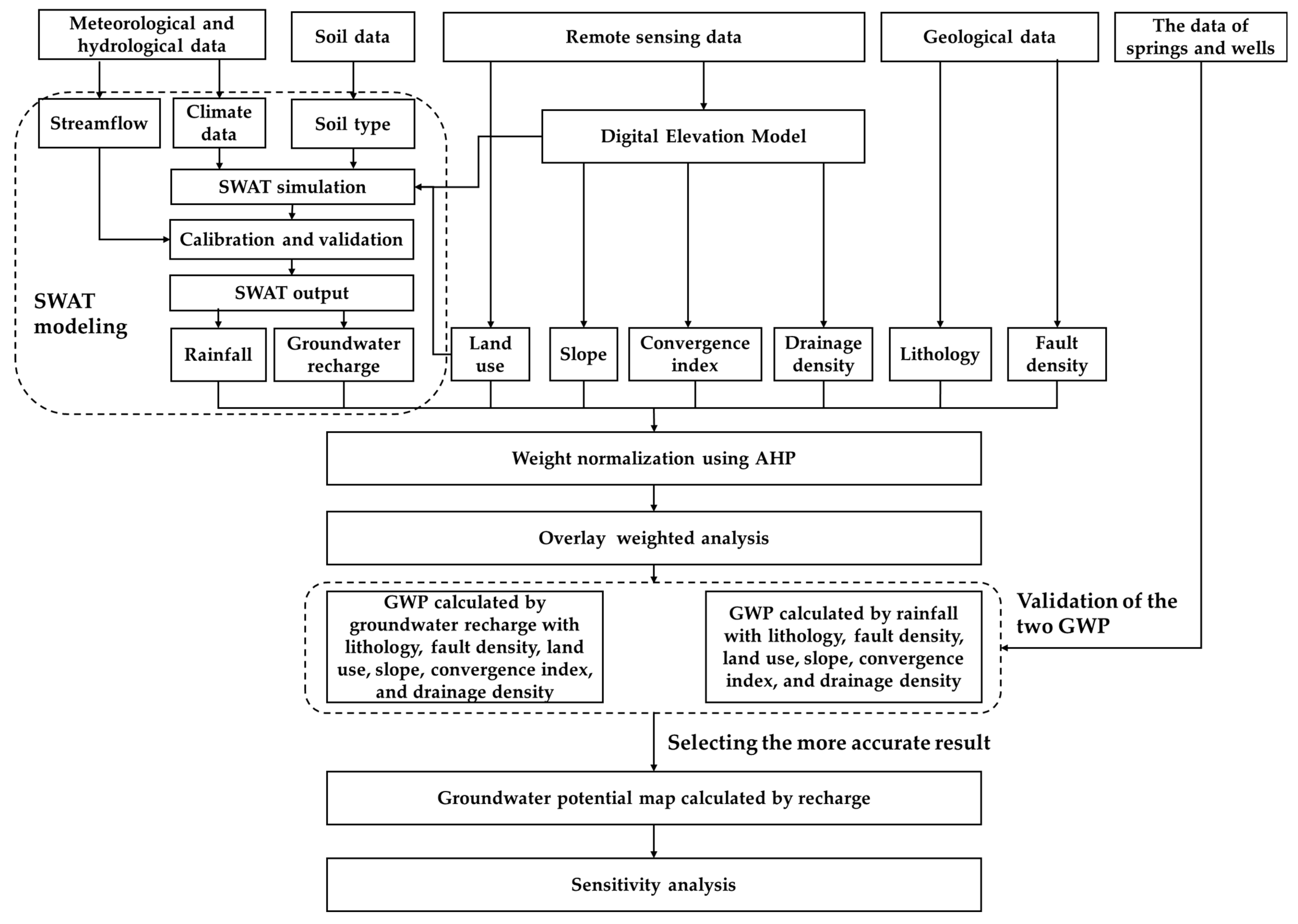
2. Materials and Methods

Figure 1 describes the method used in this research to evaluate GWP using the SWAT and AHP of multi-source data. Based on the collected meteorological, hydrological, soil, remote sensing, and geological data, eight groundwater potential assessment factors were established: lithology, fault density, land use, slope, convergence index, drainage density, rainfall, and groundwater recharge. Among them, the rainfall and recharge were estimated by the SWAT. The AHP was adopted to assign the weights of each factor, with rainfall and groundwater recharge assigned the same weight to calculate the GWP with the other six factors separately. A GWP map was generated using an overlay analysis to combine these factors, then it was validated with the data from springs and wells. The detailed experimental procedures and data processing will be described in later sections.

2.1. Study Area

The Gannan region (Figure 2) is situated in Ganzhou City, in the southern part of Jiangxi Province, between the latitudes of 25°26′ and 26°38′N and the longitudes of 114°49′ and 115°56′E. The region is characterized by numerous high mountains and hills; most of the mountains are northeast-trending, and the terrain is high in the center of the region. The predominant geomorphological type in Gannan is tectonic denudation, resulting in low hills and mountains with complex outcrops and intense tectonic activity. The region is traversed by three major rivers: the Tao River, Ping River, and Gongshui River. The region has a humid subtropical monsoon climate with unevenly distributed rainfall. The rainy season extends from March to June, accounting for approximately 55.4% of the annual rainfall. The residents of the area primarily depend on surface water.

2.2. Data Collection

Various data were collected for this research as described in Table 1. The sources of 30 m resolution DEM data were ASTER GDEM, which was utilized to construct the SWAT model and extract GWP assessment factors required for this research like slope, convergence index, and drainage density. Globeland30 [58] provided the data on land use, while the Harmonized World Soil Database (HWSD) [59] provided the soil data. These datasets were used to generate hydrological response units (HRUs) and land use was also used as a GWP assessment factor. An assimilation driving dataset called CMADS V1.1 was selected for the climate, which covered the period 2008–2016 with a daily temporal resolution and a spatial resolution of 1/4° [60]. The climate data included daily precipitation, wind speed, radiation, relative humidity, maximum temperature, and minimum temperature. It was further input into the weather generator in the SWAT model to simulate the weather conditions in the study area. The streamflow data were extracted from the Hydrological Data Yearbook of China for the SWAT model calibration and validation. The geological data used in this research can be obtained free of charge and openly through the China National Digital Geological Map website [61]. The geological data provide detailed geological information and were used to extract lithology and fault density for the GWP assessment. The well and spring data were obtained from the Wuhan Geological Survey Center of the China Geological Survey to validate the results of the GWP assessment, which included the locations of the wells and springs as well as the amount of water yielded.

2.3. Groundwater Recharge Estimation

2.3.1. Groundwater Recharge Estimation

Groundwater recharge refers to the replenishment of the groundwater volumes through a variety of means such as rainfall, subsurface runoff, and seepage from channels or rivers [62]. The SWAT has been widely employed in numerous studies worldwide to estimate groundwater recharge [53,54,55,56,57].
The SWAT is a distributed watershed hydrology model [63,64]. The model covers hydrology, soil, water quality, vegetation, meteorology, plant growth, agricultural management, and other parameters, and is currently the most representative and widely used distributed process-based model.
The SWAT model’s processes are all driven by the water balance [65]. The SWAT divides the watershed into smaller hydrological systems with watershed functions, called subbasins, which are then subdivided into different hydrological response units (HRUs) [66]. The HRU is the smallest simulation unit in the SWAT model, which is created based on a specific combination of land use, soil types, and slope [66]. There will be no water interaction between different hydrologic response units and water will not cross the subbasin, and the SWAT assumes that the areas within the same HRU have the same hydrologic cycle processes. The SWAT simulates the water cycle according to the following water balance equation [67]:
S W t = S W o + i = 1 t ( R d a y , i Q s u r f , i E a , i W s e e p , i Q g w , i )
where S W o and S W t are the initial and the final amount (mm) of water in the soil on day i; t is the time (days); R d a y , i represents the quantity (mm) of precipitation on day i; Q s u r f , i describes the measure (mm) of surface runoff on day i; E a , i is the amount (mm) of evapotranspiration on day i; W s e e p , i is the amount (mm) of water entering the vadose zone from the soil profile on day i; and Q g w , i is the amount (mm) of return flow on day i.
In the SWAT, groundwater recharge refers to the amount of water that infiltrates through the soil to the aquifers [62]. It is an important output of the SWAT. Groundwater recharge to aquifers is computed by the SWAT using the following equation [67]:
ω r c h r g , i = 1 e 1 δ g w · ω s e e p , i + e 1 δ g w · ω r c h r g , i 1
where ω r c h r g , i is the measure (mm) of water entering the aquifers on day i, δ g w is the delay time (days) of the overlying geologic formations, ω s e e p , i is the total amount (mm) of water exiting the bottom of the soil profile on day i, and ω r c h r g , i 1 is the amount (mm) of water entering the aquifers on day i − 1. The ω s e e p , i can be computed by [67]:
ω s e e p , i = ω p e r c + ω c r k , b t m
where ω p e r c is the amount (mm) of water percolating out of the lowest layer in the soil profile on day i and ω c r k , b t m is the amount (mm) of water flowing past the lower boundary of the soil profile owing to bypass flow on day i.

2.3.2. Setup for the SWAT Model

The SWAT requires a variety of data. DEM, land-use, soil, and climate data are the primary inputs of the SWAT model. The WGS 1984 UTM Zone 50N projection was used as the initial spatial dataset projection in the SWAT model setup. DEM data were used to generate digital river networks, analyze river flow directions, and delineate subbasins. Next, subbasins were divided into HRUs, consisting of a specific land use, soil type and slope. The number of HRUs depended on the set area thresholds for slope, land use and soil type [66]. Finally, 23 subbasins were created within the study area, and those subbasins were further divided into 825 HRUs with a defined slope, land use, and soil type threshold of 10%, 15%, and 10%.
After the above setup steps were completed, the climate data were input into the weather generator. The period from 2008 to 2016 was used as a simulation period, with a monthly time scale and a warm-up period of one year.

2.3.3. Calibration and Validation

Observed streamflow data from the Hanlin Bridge hydrologic station in the Ping River were collected for calibrating and validating the model in this research. The SWAT simulation was conducted for nine years, with a warm-up period in the first year, a calibration period from 2009 to 2013, and a validation period from 2014 to 2016. The SWAT parameters were only adjusted during the calibration period.
In this research, the SUFI2 algorithm in SWAT-CUP software was adopted for parameter sensitivity analyses and calibration. Through several adjustments, eleven sensitivity parameters were selected based on a global sensitivity analysis with the SUFI2 algorithm, which were CN2, SOL_AWC, GW_DELAY, APLHA_BF, ESCO, SURLAG, CH_N2, GW_REVAP, GWQMN, CANMX, and SOL_K. The parameters were modified by comparing simulated and observed streamflow data. Table 2 shows the parameters’ definitions and optimal values.
Two statistical indicators were used to evaluate the calibration and validation of the simulation: the determination coefficient ( R 2 ) and the Nash–Sutcliffe coefficient ( N S E ). These two indicators have been widely used and suggested in the SWAT model evaluation [68,69,70,71,72,73].
R 2 is a parameter used to evaluate the similarity between the observed and simulated values.
R 2 = [ i = 1 ( Q o , i Q ¯ o ) ( Q s , i Q ¯ s ) ] 2 i = 1 ( Q o , i Q ¯ o ) 2 i = 1 ( Q s , i Q ¯ s ) 2
The N S E is a parameter that is typically used to validate the simulation outcomes of hydrological models. It is used to determine how well the simulated and observed values fit together.
N S E = 1 i = 1 ( Q o , i Q s , i ) 2 i = 1 ( Q o , i Q ¯ o ) 2
In Equations (4) and (5), Q o , i and Q s , i are the observed and simulated values, and Q ¯ o and Q ¯ s are the mean of the observed and simulated values. The value of R 2 ranges from 0 to 1 and NSE takes a value of −∞–1. The model simulation is viewed as perfect if the values of R 2 and N S E equal 1. The model simulation is deemed unacceptable when the values of R 2 are close to 0 or the values of N S E are less than 0.

2.4. Groundwater Potential Assessment

2.4.1. GWP Assessment Factors

The GWP assessment factors were established using data from multiple sources. Based on an understanding of the Gannan region and findings from previous research, eight groundwater potential assessment factors were selected: lithology, fault density, land use, slope, convergence index, drainage density, rainfall, and groundwater recharge. The lithology and fault densities were extracted from the National Digital Geological Map of China Geographic Database [61]. Globeland30 provided the data on land use [58]. Slope, convergence index, and drainage density were calculated from DEM data. Rainfall and groundwater recharge were output by the SWAT model.
Lithology has an influence on the stratum’s permeability and porosity, which determines the aquifer’s ability to recharge and store water. [74]. Therefore, lithology is a significant factor affecting groundwater recharge and distribution. [75].
Faults can lead to secondary porosity, providing a channel for groundwater recharge and movement [76]. Thus, faults facilitate groundwater movement, recharge, and storage [74]. The GWP increases as the fault density increases [77]. Fault density was computed in ArcGIS, adopting a line density analysis tool.
Land use can largely determine the rate of water infiltration and surface runoff [6]. For example, woodlands and grasslands are beneficial for groundwater infiltration and recharge because extensive vegetation cover reduces evaporation and surface runoff, which in turn allows more precipitation to infiltrate the ground [77].
Slope is an important factor affecting groundwater potential [50]. There is a negative correlation between surface water infiltration and slope [78]. Steep slopes accelerate the runoff velocity and reduce infiltration, while gentle slopes facilitate surface water pooling and promote infiltration [79,80]. The slope was computed using ArcGIS based on DEM data.
Convergence index is a topographic parameter that refers to the concave shape of the terrain on a smaller spatial scale, indicating the tendency of adjacent cells toward the central cells. This index is obtained by averaging the deviation of the slope direction of the adjacent cells from the direction of the central cell, minus 90 degrees [81]. Concavities, such as valleys, are denoted by a negative value, whereas convex features, such as ridges, are denoted by a positive value, and planar areas are denoted by zero [82,83]. A detailed explanation and description of convergence index can be found in reference [81]. The convergence index was calculated based on DEM data in SAGA-GIS software [84]. SAGA-GIS calculations express this index as a percentage. The values range from −100 to 100.
Drainage density, a quantity describing the physical characteristic of a drainage basin, is the total of the surface water channel lengths per unit area and is derived from the equation [85]:
D r a i n a g e   d e n s i t y = L S
where L is the total of the surface water channel lengths (km) and S is the drainage basin area (km2). The GWP increases as the drainage density increases [25]. The channels were extracted using DEM data in ArcGIS, and then used to compute drainage density.
Rainfall is a significant source of groundwater. In general, the amount and distribution of rainfall has a large positive impact on groundwater. As a result, high rainfall regions were associated with high groundwater potential, whereas low rainfall regions were associated with low groundwater potential [86]. Rainfall was output by the SWAT model based on CMADS V1.1.
Groundwater recharge refers to the replenishment of groundwater volumes, which is a better visual representation of aquifer replenishment than rainfall. Clearly, there is a positive correlation between groundwater recharge and groundwater potential. Groundwater recharge was estimated by the SWAT model.

2.4.2. Analytic Hierarchy Process

Numerous studies have demonstrated that the analytical hierarchy process (AHP), which has been adopted in GWP assessments worldwide, has good accuracy [29,30,31,32,87,88].
In this research, the GWP assessment was performed by analyzing different GWP factors affecting groundwater movement and storage through the GIS-based AHP. The steps for determining the factor weights using the AHP are as follows: (1) defining the target (GWP); (2) constructing a square matrix to compare the relative scale between two factors depending on Saaty’s scale [27] shown in Table 3 and then assign the weights of each factor; (3) assessing the matrix consistency [89].
The comparison matrix of the AHP is as follows:
A = a 11 a 21 a 12 a 22 a 1 n a 2 n a n 1 a n 2 a n n
where a n n is the pairwise factors’ relative scale.
The normalized weights of each factor were computed using the following equation:
ω i = ( j = 1 n a i j ) 1 n k = 1 n ( j = 1 n a k j ) 1 n
The consistency of normalized weights must be examined according to the consistency ratio (CR). Only results with a CR of 10% or less are regarded as credible; otherwise, the evaluation must be adjusted to minimize inconsistencies until the CR is equal to or less than 10% [89]. The CR was computed as [89]:
  C R = C I R C I
where RCI originates from Saaty’s standard [27] shown in Table 4 and C I can be calculated according to:
C I = λ m a x n n 1
where λ m a x represents the primary eigenvalue of the A matrix.
The groundwater potential (GWP) can be calculated according to:
G W P = i = 1 n ( ω i × φ i )
where ω i and φ i represent the normalized weight and sub-classes’ rating of each factor.

2.4.3. Sensitivity Analysis

The sensitivity analysis is essential to assess the impact of each factor on the GWP results [35,79]. In the current research, the single-parameter sensitivity analysis [90] was adopted to interpret the influence of each factor on the GWP result [35,79]. This method determines the effect of each factor on the GWP result by comparing the effective weight with the empirical weight assigned to each factor. The effective weight can be calculated using the following equation:
W i = ω i × φ i G W P
where W i is the effective weight of each factor, ω i and φ i represent the normalized empirical weight and sub-classes’ rating of each factor, G W P is the groundwater potential.

3. Results

3.1. SWAT Model Output

Figure 3 and Figure 4 show graphical representations of the comparison of the monthly observed and simulated streamflow between 2009 and 2016. The results indicated that the observed and simulated values were highly correlated. The values of R 2 and N S E shown in Table 5 also supported this. Only the two values for June and July 2010 deviated significantly from each other, which was owing to the exceptionally heavy rainfall in the study area during that period.
Figure 5a,b show the spatial distribution of the mean annual rainfall and groundwater recharge during the simulation period. The graphical comparison shows a strong inconsistency in the spatial distribution. For example, in the northwest and northeast of the region, the rainfall was relatively high, but the groundwater recharge was low because of the steep slope, which makes rainfall tend to form runoff but not infiltrate the ground. In the north-central area, the groundwater recharge was high despite the relatively low rainfall because of the gentle topography and proximity to rivers. In the central part of the region, there was an overall positive correlation between rainfall and groundwater recharge. Therefore, the direct use of rainfall as a groundwater potential assessment factor in areas with complex geological features may lead to some errors.

3.2. GWP Assessment Factors

Figure 6 and Figure 7 show the eight factors that were converted to the same 30 m spatial resolution raster and projection coordinate system called WGS 1984 UTM Zone 50N for the groundwater potential assessment.
The lithology was divided into five classes based on the stratum map (Figure 6a): very poor, poor, moderate, good, and excellent for groundwater (Figure 6b). “Good” regions indicate a greater potential for groundwater, while “poor” regions indicate a lower potential. Quaternary alluvium forms a part of the “good” region where the main aquifer is a sand and pebble layer. Another part of the “good” region with high value is carboniferous rock with a high porosity. The “poor” areas are mainly Silurian and Jurassic strata with poor groundwater recharge abilities. A detailed explanation of the stratum is given in Table A1.
The fault density varied from 0 to 0.71 km/km2 (Figure 6c). Faults can provide channels for groundwater recharge and movement [76]. Thus, groundwater storage, recharge and movement are all affected by faults [74]. Therefore, in areas with high fault density, groundwater recharge and groundwater potential are considered high, while low fault density implies low groundwater recharge and potential [77].
There were seven land-use types in the region: cultivated land, forest, grassland, wetland, water bodies, artificial surfaces, and bare ground (Figure 6d). Forest and grassland can reduce evaporation and surface runoff, which can enhance the infiltration rate of precipitation [34,77]. Thus, they are associated with high groundwater potential. Conversely, artificial surfaces and bare ground have low infiltration rates owing to high evaporation and surface runoff, which is usually considered as having low groundwater potential [37,40].
The slope ranged from 0 to 63° (Figure 7a). There are many mountains in the study area with large changes in slope. In steep slope areas, rainfall is more likely to form runoff and less likely to infiltrate [36,38], while in gentle slope areas, rainfall is more likely to stay on the surface and has more time to infiltrate [35,38]. Thus, high slope values lead to high surface runoff and low infiltration, which are associated with low groundwater potential. And low slope values are associated with high groundwater potential owing to high infiltration.
The convergence index lay within the range of −100 and 99.26 (Figure 7b). The effect of the convergence index on groundwater is similar to that of slope. Negative values indicate depressions in the terrain, which are favorable for infiltration, while positive values indicate convex features, which lead to high runoff and low infiltration [50]. Therefore, areas with high convergence index values have high groundwater potential, while areas with low values have low potential.
The drainage density ranged from 0 to 0.78 km/km2 (Figure 7c). Regions with high drainage density were mostly near major rivers, where groundwater is more likely to be recharged by rivers. Areas with low drainage density were mainly in the bedrock mountains, which is not conducive to infiltration. For this reason, areas with high drainage density are considered as having high groundwater potential, while areas with low density have low potential.
The annual rainfall varied from 1438 to 1603 mm (Figure 7d). High rainfall was mainly concentrated in the northwest, northeast, and south-central regions. The annual groundwater recharge ranged from 369 to 685 mm (Figure 7e). High recharge was mainly concentrated in the north-central area. Both of the factors were assigned high weights for high values.

3.3. GWP Map

The weights of the eight factors were obtained by the hierarchical analysis method (Table 6). The CR of 9.7% (less than 10%) indicated that the matrix was consistent. The GWP was calculated by an overlay analysis (Equation (11)) based on the weights calculated by the AHP (Table 6) and sub-classes’ rating of each factor (Table 7), with rainfall and groundwater recharge assigned the same weight to calculate the GWP with the other six factors separately.
The region was divided into five classes based on the result of groundwater potential (Figure 8). The data from 23 wells and 42 springs collected by the Wuhan Geological Survey Center were used to validate the GWP. A correlation analysis was conducted between groundwater potential and flow rates of wells and springs, with the spring flow rate taken as a logarithm because of the wide range in the values. The results are shown in Figure 9 and Figure 10. There was a strong exponential relationship between the GWP calculated by recharge and well yield (R2 = 0.8), while there was no significant correlation between the GWP calculated by rainfall and well yield (R2 = 0.21) (Figure 9). The GWP calculated by groundwater recharge showed a strong positive correlation with the spring discharge (R2 = 0.74), while the GWP calculated by rainfall only showed a weak positive correlation with the spring discharge (R2 = 0.48) (Figure 10). The data comparison results indicated that the GWP calculated by groundwater recharge can more reasonably predict the actual groundwater potential. Therefore, the GWP calculated by the groundwater recharge (Figure 8a) is more accurate.
The study area was divided into five classes based on the GWP calculated by the groundwater recharge (Figure 8a): very poor, poor, moderate, good, and excellent, accounting for 15.22%, 27.73%, 27.31%, 20.44%, and 9.3%, respectively. The “good” areas are mostly located in the valley plains near rivers. The gentle slopes, proximity to rivers, and the predominantly loose sandstone and conglomerate lithology of the “good” areas make the area favorable for aquifer replenishment. The “poor” areas are mainly in mountainous regions with steep slopes and bedrock, which are not favorable for aquifer replenishment.

3.4. Sensitivity Analysis

The results of the single-parameter sensitivity analysis are shown in Table 8. The results showed some deviations between the effective and empirical weights. The single-parameter sensitivity analysis showed that slope was the most effective factor with a mean effective weight of 21.57%. The drainage density, lithology, land use, and recharge were the next higher mean effective weights of 15.04%, 14.97%, 14.48%, and 13.38%. The convergence index and fault density exhibited lower mean effective weights of 11.12% and 9.44%. The effective and empirical weights for the recharge, land use, convergence index and fault density were found to be close to each other.
Although showing some deviations between the effective and empirical weights, the three most effective factors were still slope, drainage, and lithology. This further illustrates the importance of these three factors in the GWP assessment.

4. Discussion

The factors selected for GWP assessment in previous studies were basically limited to geology, hydrology, topography, and aquifer replenishment [34,35,36,37,38,39,40,41,42,43,44,45,46,47]. The selection of factors from geology, hydrology, and topography differed according to the geological background of the study area [34,35,36,37,38,39,40,41,42,43,44,45,46,47,86,87,88]. However, in terms of aquifer replenishment, researchers have mostly focused on rainfall rather than groundwater recharge [50,51,52]. In this research, the groundwater recharge estimated using the SWAT was compared with rainfall and incorporated into the GWP assessment. The comparison between groundwater recharge and rainfall showed a large inconsistency in spatial distribution between them, indicating that rainfall is not representative of groundwater recharge in areas with complex geological features (Figure 5). The comparison of the GWP results further illustrated that the direct use of rainfall as a groundwater potential assessment factor in areas with a wide range of geological features can lead to some errors (Figure 9 and Figure 10). This is because the conversion of rainfall to groundwater is influenced by various factors, such as soil, lithology, and topography.
The study area was divided into five classes based on the GWP assessment results: very poor, poor, moderate, good, and excellent. Excellent areas and good areas accounted for 9.30% and 20.44% of the study area, respectively. These areas primarily consist of loose sandstone and conglomerates with high permeability, enabling effective groundwater recharge. Topographically, their slopes are relatively gentle and belong to the erosion–accumulation valley/plain landforms. From a hydrological aspect, the areas are near surface rivers, which are well recharged. Areas with a moderate GWP accounted for 27.31% and are mainly located in the hills where the plains and mountains meet, with sparse vegetation and a complex geological environment. Here, the groundwater recharge depends on rainfall. Areas with a poor GWP and a very poor GWP accounted for 27.73% and 15.22%, respectively. These areas are mostly located in the mountains and consist of brittle granite with low permeability. These areas have steep slopes and almost no streams, which is not conducive to groundwater recharge.
For this study area, the groundwater in high altitude mountainous areas is mostly bedrock fracture water, and the groundwater potential is often low. Limited by the complex topography, limited transportation bedrock areas are not recommended as groundwater development areas. In contrast, in the valley or plain area near the river the GWP is high and the ground is mainly loose sandstone and distributed conglomerate. In addition, the convenient transportation and relative proximity to residential areas make it a more ideal location for groundwater development.
The results show that using groundwater recharge estimated by the SWAT improved the accuracy of the GWP assessment. Groundwater recharge is a better visual representation of aquifer replenishment than rainfall. However, the method still has some limitations. The streamflow data for calibration and validation of the SWAT are not easily accessible owing to confidentiality. Furthermore, only water yield data were used to validate the GWP results without considering the groundwater level owing to data limitations. In the future, the groundwater level fluctuation variation with the amount of rainfall, ET, and groundwater recharge will be considered to improve the GWP assessment.

5. Conclusions

In this research, the GWP of the Gannan region was calculated using the SWAT model and GIS-based AHP. Data preparation for the research was completed using ArcGIS. The simulation results of the SWAT model were calibrated and validated using observed streamflow data from the Hanlin Bridge hydrologic station on the Ping River. The values of R 2 and N S E indicated that the model was accurate and reasonable and can be used to simulate the water cycle in the region. Then, the model was used to estimate groundwater recharge. The results showed the differences in the spatial distribution of rainfall and groundwater recharge, indicating that the direct use of rainfall as a groundwater potential assessment factor in areas with complex geological features may lead to some errors. To better compare the effects of rainfall and groundwater recharge on GWP, the AHP was adopted to assign the weights to each factor, with rainfall and groundwater recharge assigned the same weight to calculate the GWP with the other six factors (lithology, fault density, land use, slope, convergence index, and drainage density) separately. A correlation analysis was performed between the groundwater potential and the flow rates of wells and springs to validate the assessment results. The data comparison results showed that the GWP calculated by groundwater recharge was more accurate. Depending on the GWP assessment results, the Gannan region was split into five classes: very poor, poor, moderate, good, and excellent. “Good” areas were mostly located near rivers and were suggested as sites for groundwater exploitation because of the favorable slope (gentle terrain), lithology (loose sediments), and recharge. “Poor” areas were mainly mountainous areas with poor geological environments (e.g., steep slopes and bedrock).
Experimental results showed that the GIS-based AHP can effectively identify groundwater potential zones, and the combination of the SWAT and AHP can enable a significant increase in the accuracy of the method in data-scarce areas. By using this method, it is easy to identify the potential area of groundwater, thus saving a lot of manpower and time. It also solves the problem of using a lot of time and energy to carry out field exploration. This research contributes to groundwater exploration, exploitation, and management. This method can be used as a reference for other water-scarce areas with complicated geological backgrounds. Depending on the results of the GWP assessment, policy makers can better formulate policies for groundwater.

Author Contributions

Conceptualization, methodology, and formal analysis, Z.Z., S.Z., M.L. and Y.Z.; software, validation, and visualization, Z.Z.; investigation, resources, and data curation, Z.Z., M.C., Q.Z., Z.D. and J.L.; writing—original draft preparation, Z.Z.; writing—review and editing and supervision, S.Z. and Y.Z. All authors have read and agreed to the published version of the manuscript.

Funding

This research was funded by the National Natural Science Foundation of China (grant number U1939204, 42074176, and 41874169) and the National Key R&D Program of China (grant number 2020YFC1512401).

Data Availability Statement

The DEM data are openly available on the Geospatial Data Cloud site (http://www.gscloud.cn accessed on 24 November 2022). The soil type data can be downloaded here: (https://www.fao.org/soils-portal/data-hub/soil-maps-and-databases/harmonized-world-soil-database-v12/en/ accessed on 15 December 2022). The land-use data can be found here: (http://www.globalland30.com/ accessed on 24 November 2022). The climate data can be downloaded here: (http://www.cmads.org/ accessed on 20 December 2022). The geological data used in this paper can be obtained free of charge through the China National Digital Geological Map website (https://www.ngac.cn/125cms/c/qggnew/index.htm accessed on 15 November 2022). The streamflow, well, and spring data are subject to confidentiality regulations and are not publicly available.

Acknowledgments

The authors are grateful to the Wuhan Geological Survey Center for providing validation data. The first author would like to thank Shuangxi Zhang and Yu Zhang for their suggestions for this research. We thank the editors and reviewers for their constructive comments and suggestions to improve our manuscript.

Conflicts of Interest

The authors declare no conflict of interest.

Appendix A

Table A1. Stratigraphic information of the study area.
StratumAbbreviationDescription
Niugouhe Formation of Cambrian 1 Slate, sandstone, and carbonaceous slate
Gautan Formation of Cambrian 2 Sandstone, slate, and siltstone
Shuishi Formation of Cambrian 3 Slate, sandstone, and carbonaceous slate
Zishan Formation of Carboniferous C 1 Conglomerate and sandstone
Hutian Group of Carboniferous C 2 P 1 Dolomite and biotite
Yunshan Formation, Zhongpeng Formation, and Luoduan Formation, Xiashan Group, Devonian D 2 Conglomerates, sandstones, siltstones, and siltstones
Yunshan Formation, Zhongpeng Formation, and Zhangdong Formation, Xiashan Group, Devonian D 3 Conglomerate and sandstone
Xiashan Formation, Zhangdong Formation, and Zishan Formation, Xiashan Group, Devonian D 3 C 1 Siltstone, mudstone, sandstone, siltstone, and shale
Beishui Formation, Linshan Group, Jurassic J 1 Sandstone, gravelly sandstone, fine sandstone, and siltstone
Luoao Formation J 2 Sandstone, siltstone, and conglomerate
Huobashan Group of Cretaceous K 1 2 Limestone, siltstone, and conglomerate
Hekou Formation and Tangbian Formation, Ganzhou Group, Cretaceous K 2 Conglomerates, sandstones, greywacke, and basalt
Yangjiaqiao Formation of Nanhua N h Mud conglomerate, quartzite, and sand conglomerate
Chetou Formation, Liangshan Formation, Qixia Formation, Xiaojiangbian Formation and Maokou Formation of Permian P 2 Siltstone, shale, and limestone
Leping Formation, Changxing Formation, and Dalong Formation of Permian P 3 Granite
Tantou Formation of Quaternary Q b 2 T Granite
Lianyu Group of Quaternary Q h f Granite
Water Body Q h w Granite
Ganxian Formation of Quaternary Q p 1 f p Granite
Anyuan Group of Triassic T 3 Granite
Lechangxia Group of Sinian Z Granite
Early Jurassic Granites γ J 1 Granite
Gexianshan Upper Unit of Middle Jurassic γ J 2 Granite
Shangyou Upper Unit of Late Silurian γ S 3 Granite
Qiaotou Upper Unit, Qingxi Upper Unit, Fucheng Upper Unit, and Tuqiao Upper Unit of Late Triassic γ T 3 Granite
Huping Upper Unit and Laoluopi Upper Unit of Late Silurian γ δ ο S 3 Granite
Fengshi Upper Unit of Early Jurassic η γ J 1 Granite
Lingshan Upper Unit, Yuexing Upper Unit, Mazitang Upper Unit, and Hengshan Upper Unit of Middle Jurassic η γ J 2 Granite
Black Mica Diorite Granite of Late Jurassic η γ J 3 Granite
Fufang Upper Unit and Tanghu Upper Unit of Middle Silurian η γ S 2 Granite
Guikeng Upper Unit, Huping Upper Unit, and Shangyou Upper Unit of Late Silurian η γ S 3 Granite
Fucheng Upper Unit, Qingxi Upper Unit, Qiaotou Upper Unit, and Yujingshan Upper Unit of Late Triassic η γ T 3 Granite
Shangyou Upper Unit of Late Silurian ξ γ J 2 Granite

References

  1. Oki, T.; Kanae, S. Global hydrological cycles and world water resources. Science 2006, 313, 1068–1072. [Google Scholar] [CrossRef] [Green Version]
  2. Osman, A.I.A.; Ahmed, A.N.; Chow, M.F.; Huang, Y.F.; El-Shafie, A. Extreme gradient boosting (Xgboost) model to predict the groundwater levels in Selangor Malaysia. Ain Shams Eng. J. 2021, 12, 1545–1556. [Google Scholar] [CrossRef]
  3. Osman, A.I.A.; Ahmed, A.N.; Huang, Y.F.; Kumar, P.; Birima, A.H.; Sherif, M.; Sefelnasr, A.; Ebraheemand, A.A.; El-Shafie, A. Past, present and perspective methodology for groundwater modeling-based machine learning approaches. Arch. Comput. Method Eng. 2022, 29, 3843–3859. [Google Scholar] [CrossRef]
  4. Water, U.N. Groundwater: Making the invisible visible. Legal Lock J. 2022, 1, 69. [Google Scholar]
  5. Naghibi, S.A.; Moghaddam, D.D.; Kalantar, B.; Pradhan, B.; Kisi, O. A comparative assessment of GIS-based data mining models and a novel ensemble model in groundwater well potential mapping. J. Hydrol. 2017, 548, 471–483. [Google Scholar] [CrossRef]
  6. Ammar, A.I.; Kamal, K.A. Resistivity method contribution in determining of fault zone and hydro-geophysical characteristics of carbonate aquifer, eastern desert, Egypt. Appl. Water Sci. 2018, 8, 1–27. [Google Scholar] [CrossRef] [Green Version]
  7. Allafta, H.; Opp, C.; Patra, S. Identification of groundwater potential zones using remote sensing and GIS techniques: A case study of the Shatt Al-Arab Basin. Remote Sens. 2020, 13, 112. [Google Scholar]
  8. Moss, R.; Moss, G.E. Handbook of Ground Water Development; Wiley-Interscience: New York, NY, USA, 1990. [Google Scholar]
  9. Fetter, C.W. Applied Hydrogeology; Waveland Press: Long Grove, IL, USA, 2018. [Google Scholar]
  10. Elmahdy, S.I.; Mohamed, M.M. Automatic detection of near surface geological and hydrological features and investigating their influence on groundwater accumulation and salinity in southwest Egypt using remote sensing and GIS. Geocarto Int. 2015, 30, 132–144. [Google Scholar] [CrossRef]
  11. Elfadaly, A.; Attia, W.; Lasaponara, R. Monitoring the environmental risks around Medinet Habu and Ramesseum Temple at West Luxor, Egypt, using remote sensing and GIS techniques. J. Archaeol. Method Theory 2018, 25, 587–610. [Google Scholar] [CrossRef]
  12. Díaz-Alcaide, S.; Martínez-Santos, P. Advances in groundwater potential mapping. Hydrogeol. J. 2019, 27, 2307–2324. [Google Scholar] [CrossRef]
  13. Elbeih, S.F. An overview of integrated remote sensing and GIS for groundwater mapping in Egypt. Ain Shams Eng. J. 2015, 6, 1–15. [Google Scholar] [CrossRef] [Green Version]
  14. Agarwal, E.; Agarwal, R.; Garg, R.D.; Garg, P.K. Delineation of groundwater potential zone: An AHP/ANP approach. J. Earth Syst. Sci. 2013, 122, 887–898. [Google Scholar]
  15. Abrams, W.; Ghoneim, E.; Shew, R.; LaMaskin, T.; Al-Bloushi, K.; Hussein, S.; AbuBakr, M.; Al-Mulla, E.; Al-Awar, M.; El-Baz, F. Delineation of groundwater potential (GWP) in the northern United Arab Emirates and Oman using geospatial technologies in conjunction with Simple Additive Weight (SAW), Analytical Hierarchy Process (AHP), and Probabilistic Frequency Ratio (PFR) techniques. J. Arid. Environ. 2018, 157, 77–96. [Google Scholar]
  16. Thapa, R.; Gupta, S.; Gupta, A.; Reddy, D.V.; Kaur, H. Use of geospatial technology for delineating groundwater potential zones with an emphasis on water-table analysis in Dwarka River basin, Birbhum, India. Hydrogeol. J. 2018, 26, 899–922. [Google Scholar] [CrossRef]
  17. Manikandan, J.; Kiruthika, A.M.; Sureshbabu, S. Evaluation of groundwater potential zones in Krishnagiri District, Tamil Nadu using MIF Technique. Int. J. Innov. Res. Sci. Eng. Technol. 2014, 3, 10524–10534. [Google Scholar]
  18. Mohammadi-Behzad, H.R.; Charchi, A.; Kalantari, N.; Nejad, A.M.; Vardanjani, H.K. Delineation of groundwater potential zones using remote sensing (RS), geographical information system (GIS) and analytic hierarchy process (AHP) techniques: A case study in the Leylia–Keynow watershed, southwest of Iran. Carbonates Evaporites 2019, 34, 1307–1319. [Google Scholar]
  19. Ozdemir, A. GIS-based groundwater spring potential mapping in the Sultan Mountains (Konya, Turkey) using frequency ratio, weights of evidence and logistic regression methods and their comparison. J. Hydrol. 2011, 411, 290–308. [Google Scholar]
  20. Oh, H.; Kim, Y.; Choi, J.; Park, E.; Lee, S. GIS mapping of regional probabilistic groundwater potential in the area of Pohang City, Korea. J. Hydrol. 2011, 399, 158–172. [Google Scholar]
  21. Naghibi, S.A.; Pourghasemi, H.R.; Dixon, B. GIS-based groundwater potential mapping using boosted regression tree, classification and regression tree, and random forest machine learning models in Iran. Environ. Monit. Assess. 2016, 188, 44. [Google Scholar]
  22. Guru, B.; Seshan, K.; Bera, S. Frequency ratio model for groundwater potential mapping and its sustainable management in cold desert, India. J. King Saud Univ.-Sci. 2017, 29, 333–347. [Google Scholar]
  23. Lee, S.; Kim, Y.; Oh, H. Application of a weights-of-evidence method and GIS to regional groundwater productivity potential mapping. J. Environ. Manag. 2012, 96, 91–105. [Google Scholar] [CrossRef] [PubMed]
  24. Duan, H.; Deng, Z.; Deng, F.; Wang, D. Assessment of groundwater potential based on multicriteria decision making model and decision tree algorithms. Math. Probl. Eng. 2016, 2016, 2064575. [Google Scholar]
  25. Das, S. Comparison among influencing factor, frequency ratio, and analytical hierarchy process techniques for groundwater potential zonation in Vaitarna basin, Maharashtra, India. Groundw. Sustain. Dev. 2019, 8, 617–629. [Google Scholar]
  26. Chen, W.; Li, H.; Hou, E.; Wang, S.; Wang, G.; Panahi, M.; Li, T.; Peng, T.; Guo, C.; Niu, C. GIS-based groundwater potential analysis using novel ensemble weights-of-evidence with logistic regression and functional tree models. Sci. Total Environ. 2018, 634, 853–867. [Google Scholar]
  27. Saaty, R.W. The analytic hierarchy process—What it is and how it is used. Math. Model. 1987, 9, 161–176. [Google Scholar] [CrossRef] [Green Version]
  28. Finizio, A.; Villa, S. Environmental risk assessment for pesticides: A tool for decision making. Environ. Impact Assess. Rev. 2002, 22, 235–248. [Google Scholar]
  29. Arulbalaji, P.; Padmalal, D.; Sreelash, K. GIS and AHP techniques based delineation of groundwater potential zones: A case study from southern Western Ghats, India. Sci. Rep. 2019, 9, 2082. [Google Scholar]
  30. Saranya, T.; Saravanan, S. Groundwater potential zone mapping using analytical hierarchy process (AHP) and GIS for Kancheepuram District, Tamilnadu, India. Model. Earth Syst. Environ. 2020, 6, 1105–1122. [Google Scholar]
  31. Nithya, C.N.; Srinivas, Y.; Magesh, N.S.; Kaliraj, S. Assessment of groundwater potential zones in Chittar basin, Southern India using GIS based AHP technique. Remote Sens. Appl. Soc. Environ. 2019, 15, 100248. [Google Scholar] [CrossRef]
  32. Achu, A.L.; Thomas, J.; Reghunath, R. Multi-criteria decision analysis for delineation of groundwater potential zones in a tropical river basin using remote sensing, GIS and analytical hierarchy process (AHP). Groundw. Sustain. Dev. 2020, 10, 100365. [Google Scholar]
  33. Bera, A.; Mukhopadhyay, B.P.; Barua, S. Delineation of groundwater potential zones in Karha river basin, Maharashtra, India, using AHP and geospatial techniques. Arab. J. Geosci. 2020, 13, 693. [Google Scholar]
  34. Genjula, W.; Jothimani, M.; Gunalan, J.; Abebe, A. Applications of statistical and AHP models in groundwater potential mapping in the Mensa river catchment, Omo river valley, Ethiopia. Model. Earth Syst. Environ. 2023, 1–19. [Google Scholar] [CrossRef]
  35. Mahato, R.; Bushi, D.; Nimasow, G.; Nimasow, O.D.; Joshi, R.C. AHP and GIS-based delineation of groundwater potential of Papum Pare District of Arunachal Pradesh, India. J. Geol. Soc. India 2022, 98, 102–112. [Google Scholar]
  36. Moharir, K.N.; Pande, C.B.; Gautam, V.K.; Singh, S.K.; Rane, N.L. Integration of hydrogeological data, GIS and AHP techniques applied to delineate groundwater potential zones in sandstone, limestone and shales rocks of the Damoh district,(MP) central India. Environ. Res. 2023, 228, 115832. [Google Scholar] [PubMed]
  37. Ashwini, K.; Verma, R.K.; Sriharsha, S.; Chourasiya, S.; Singh, A. Delineation of groundwater potential zone for sustainable water resources management using remote sensing-GIS and analytic hierarchy approach in the state of Jharkhand, India. Groundw. Sustain. Dev. 2023, 21, 100908. [Google Scholar]
  38. Arumugam, M.; Kulandaisamy, P.; Karthikeyan, S.; Thangaraj, K.; Senapathi, V.; Chung, S.Y.; Muthuramalingam, S.; Rajendran, M.; Sugumaran, S.; Manimuthu, S. An Assessment of Geospatial Analysis Combined with AHP Techniques to Identify Groundwater Potential Zones in the Pudukkottai District, Tamil Nadu, India. Water 2023, 15, 1101. [Google Scholar]
  39. Gautam, V.K.; Pande, C.B.; Kothari, M.; Singh, P.K.; Agrawal, A. Exploration of groundwater potential zones mapping for hard rock region in the Jakham river basin using geospatial techniques and aquifer parameters. Adv. Space Res. 2023, 71, 2892–2908. [Google Scholar]
  40. Etuk, M.N.; Igwe, O.; Egbueri, J.C. An integrated geoinformatics and hydrogeological approach to delineating groundwater potential zones in the complex geological terrain of Abuja, Nigeria. Model. Earth Syst. Environ. 2023, 9, 285–311. [Google Scholar]
  41. Ikirri, M.; Boutaleb, S.; Ibraheem, I.M.; Abioui, M.; Echogdali, F.Z.; Abdelrahman, K.; Id-Belqas, M.; Abu-Alam, T.; El Ayady, H.; Essoussi, S. Delineation of Groundwater Potential Area using an AHP, Remote Sensing, and GIS Techniques in the Ifni Basin, Western Anti-Atlas, Morocco. Water 2023, 15, 1436. [Google Scholar]
  42. Yadav, B.; Malav, L.C.; Jangir, A.; Kharia, S.K.; Singh, S.V.; Yeasin, M.; Nogiya, M.; Meena, R.L.; Meena, R.S.; Tailor, B.L. Application of analytical hierarchical process, multi-influencing factor, and geospatial techniques for groundwater potential zonation in a semi-arid region of western India. J. Contam. Hydrol. 2023, 253, 104122. [Google Scholar]
  43. Danso, S.Y.; Ma, Y. Geospatial techniques for groundwater potential zones delineation in a coastal municipality, Ghana. Egypt. J. Remote Sens. Space Sci. 2023, 26, 75–84. [Google Scholar]
  44. Goswami, A.; Gor, N.; Borah, A.J.; Chauhan, G.; Saha, D.; Kothyari, G.C.; Barpatra, D.; Hazarika, A.; Lakhote, A.; Jani, C. Groundwater potential zone demarcation in the Khadir Island of Kachchh, Western India. Groundw. Sustain. Dev. 2023, 20, 100876. [Google Scholar]
  45. Petrick, N.; Jubidi, M.F.B.; Ahmad Abir, I. Groundwater Potential Assessment of Penang Island, Malaysia, Through Integration of Remote Sensing and GIS with Validation by 2D ERT. Nat. Resour. Res. 2023, 32, 523–541. [Google Scholar]
  46. Ifediegwu, S.I. Assessment of groundwater potential zones using GIS and AHP techniques: A case study of the Lafia district, Nasarawa State, Nigeria. Appl. Water Sci. 2022, 12, 10. [Google Scholar] [CrossRef]
  47. Melese, T.; Belay, T. Groundwater potential zone mapping using analytical hierarchy process and GIS in Muga Watershed, Abay Basin, Ethiopia. Glob. Chall. 2022, 6, 2100068. [Google Scholar] [CrossRef]
  48. Kaur, L.; Rishi, M.S. Integrated geospatial, geostatistical, and remote-sensing approach to estimate groundwater level in North-western India. Environ. Earth Sci. 2018, 77, 786. [Google Scholar] [CrossRef]
  49. Wakode, H.B.; Baier, K.; Jha, R.; Azzam, R. Impact of urbanization on groundwater recharge and urban water balance for the city of Hyderabad, India. Int. Soil Water Conserv. Res. 2018, 6, 51–62. [Google Scholar] [CrossRef]
  50. Zhang, Q.; Zhang, S.; Zhang, Y.; Li, M.; Wei, Y.; Chen, M.; Zhang, Z.; Dai, Z. GIS-Based Groundwater Potential Assessment in Varied Topographic Areas of Mianyang City, Southwestern China, Using AHP. Remote Sens. 2021, 13, 4684. [Google Scholar] [CrossRef]
  51. Mallick, J.; Khan, R.A.; Ahmed, M.; Alqadhi, S.D.; Alsubih, M.; Falqi, I.; Hasan, M.A. Modeling groundwater potential zone in a semi-arid region of Aseer using fuzzy-AHP and geoinformation techniques. Water 2019, 11, 2656. [Google Scholar]
  52. Yifru, B.A.; Mitiku, D.B.; Tolera, M.B.; Chang, S.W.; Chung, I. Groundwater potential mapping using SWAT and GIS-based multi-criteria decision analysis. KSCE J. Civ. Eng. 2020, 24, 2546–2559. [Google Scholar]
  53. Githui, F.; Selle, B.; Thayalakumaran, T. Recharge estimation using remotely sensed evapotranspiration in an irrigated catchment in southeast Australia. Hydrol. Process. 2012, 26, 1379–1389. [Google Scholar]
  54. Jin, G.; Shimizu, Y.; Onodera, S.; Saito, M.; Matsumori, K. Evaluation of drought impact on groundwater recharge rate using SWAT and Hydrus models on an agricultural island in western Japan. Proc. Int. Assoc. Hydrol. Sci. 2015, 371, 143–148. [Google Scholar]
  55. Awan, U.K.; Ismaeel, A. A new technique to map groundwater recharge in irrigated areas using a SWAT model under changing climate. J. Hydrol. 2014, 519, 1368–1382. [Google Scholar] [CrossRef]
  56. Eshtawi, T.; Evers, M.; Tischbein, B. Quantifying the impact of urban area expansion on groundwater recharge and surface runoff. Hydrol. Sci. J. 2016, 61, 826–843. [Google Scholar] [CrossRef]
  57. Putthividhya, A.; Laonamsai, J. SWAT and MODFLOW modeling of spatio-temporal runoff and groundwater recharge distribution. In World Environmental and Water Resources Congress; ASCE Press: Reston, VA, USA, 2017; Volume 2017, pp. 51–65. [Google Scholar]
  58. Jun, C.; Ban, Y.; Li, S. Open access to Earth land-cover map. Nature 2014, 514, 434. [Google Scholar] [CrossRef] [Green Version]
  59. Fischer, G.; Nachtergaele, F.; Prieler, S.; Van Velthuizen, H.T.; Verelst, L.; Wiberg, D. Global Agro-Ecological Zones Assessment for Agriculture (GAEZ 2008); IIASA: Laxenburg, Austria; FAO: Rome, Italy, 2008; Volume 10. [Google Scholar]
  60. Meng, X.; Wang, H. China meteorological assimilation driving datasets for the SWAT model Version 1.1 (2008–2016). Natl. Tibet. Plateau Data Cent. 2018. [Google Scholar] [CrossRef]
  61. Li, C.Y.; Wang, X.C.; He, C.Z.; Wu, X.; Kong, Z.Y.; Li, X.L. China National Digital Geological Map (Public Version at 1: 200 000 Scale) Spatial Database (V1). China Geol. Surv. 2017, 46, 1–10. [Google Scholar]
  62. Freeze, R.A.; Cherry, J.A. Groundwater; Prentice-Hall: Hoboken, NJ, USA, 1977. [Google Scholar]
  63. Gassman, P.W.; Sadeghi, A.M.; Srinivasan, R. Applications of the SWAT model special section: Overview and insights. J. Environ. Qual. 2014, 43, 1–8. [Google Scholar] [PubMed]
  64. Arnold, J.G.; Srinivasan, R.; Muttiah, R.S.; Williams, J.R. Large area hydrologic modeling and assessment part I: Model development 1. JAWRA J. Am. Water Resour. Assoc. 1998, 34, 73–89. [Google Scholar]
  65. Ayivi, F.; Jha, M.K. Estimation of water balance and water yield in the Reedy Fork-Buffalo Creek Watershed in North Carolina using SWAT. Int. Soil Water Conserv. Res. 2018, 6, 203–213. [Google Scholar] [CrossRef]
  66. Ridwansyah, I.; Yulianti, M.; Onodera, S.; Shimizu, Y.; Wibowo, H.; Fakhrudin, M. The impact of land use and climate change on surface runoff and groundwater in Cimanuk watershed, Indonesia. Limnology 2020, 21, 487–498. [Google Scholar]
  67. Neitsch, S.L.; Arnold, J.G.; Kiniry, J.R.; Williams, J.R. Soil and Water Assessment Tool Theoretical Documentation Version 2009; Texas Water Resources Institute: College Station, TX, USA, 2011. [Google Scholar]
  68. Bennour, A.; Jia, L.; Menenti, M.; Zheng, C.; Zeng, Y.; Asenso Barnieh, B.; Jiang, M. Calibration and validation of SWAT model by using hydrological remote sensing observables in the Lake Chad Basin. Remote Sens. 2022, 14, 1511. [Google Scholar]
  69. Liu, Z.; Rong, L.; Wei, W. Impacts of land use/cover change on water balance by using the SWAT model in a typical loess hilly watershed of China. Geogr. Sustain. 2023, 4, 19–28. [Google Scholar]
  70. Sharma, A.; Patel, P.L.; Sharma, P.J. Influence of climate and land-use changes on the sensitivity of SWAT model parameters and water availability in a semi-arid river basin. Catena 2022, 215, 106298. [Google Scholar]
  71. Son, N.T.; Le Huong, H.; Loc, N.D.; Phuong, T.T. Application of SWAT model to assess land use change and climate variability impacts on hydrology of Nam Rom Catchment in Northwestern Vietnam. Environ. Dev. Sustain. 2022, 24, 3091–3109. [Google Scholar]
  72. Trivedi, A.; Awasthi, M.K.; Gautam, V.K.; Pande, C.B.; Din, N.M. Evaluating the groundwater recharge requirement and restoration in the Kanari river, India, using SWAT model. In Environment, Development and Sustainability; Springer: Berlin/Heidelberg, Germany, 2023; pp. 1–26. [Google Scholar]
  73. Pandi, D.; Kothandaraman, S.; Kuppusamy, M. Simulation of water balance components using SWAT model at sub catchment level. Sustainability 2023, 15, 1438. [Google Scholar]
  74. Al-Djazouli, M.O.; Elmorabiti, K.; Rahimi, A.; Amellah, O.; Fadil, O.A.M. Delineating of groundwater potential zones based on remote sensing, GIS and analytical hierarchical process: A case of Waddai, eastern Chad. GeoJournal 2021, 86, 1881–1894. [Google Scholar]
  75. Kaur, L.; Rishi, M.S.; Singh, G.; Thakur, S.N. Groundwater potential assessment of an alluvial aquifer in Yamuna sub-basin (Panipat region) using remote sensing and GIS techniques in conjunction with analytical hierarchy process (AHP) and catastrophe theory (CT). Ecol. Indic. 2020, 110, 105850. [Google Scholar]
  76. Pinto, D.; Shrestha, S.; Babel, M.S.; Ninsawat, S. Delineation of groundwater potential zones in the Comoro watershed, Timor Leste using GIS, remote sensing and analytic hierarchy process (AHP) technique. Appl. Water Sci. 2017, 7, 503–519. [Google Scholar] [CrossRef] [Green Version]
  77. Mukherjee, I.; Singh, U.K. Assessment of fluoride contaminated groundwater on food crops and vegetables in Birbhum District of West Bengal, India. In Advance Technologies in Agriculture for Doubling Farmer’s Income; New Delhi Publishers: New Delhi, India, 2018; pp. 225–235. [Google Scholar]
  78. Oikonomidis, D.; Dimogianni, S.; Kazakis, N.; Voudouris, K. A GIS/remote sensing-based methodology for groundwater potentiality assessment in Tirnavos area, Greece. J. Hydrol. 2015, 525, 197–208. [Google Scholar]
  79. Mukherjee, I.; Singh, U.K. Delineation of groundwater potential zones in a drought-prone semi-arid region of east India using GIS and analytical hierarchical process techniques. Catena 2020, 194, 104681. [Google Scholar] [CrossRef]
  80. Yang, J.; Zhang, H.; Ren, C.; Nan, Z.; Wei, X.; Li, C. A cross-reconstruction method for step-changed runoff series to implement frequency analysis under changing environment. Int. J. Environ. Res. Public Health 2019, 16, 4345. [Google Scholar] [CrossRef] [PubMed] [Green Version]
  81. Kiss, R. Determination of drainage network in digital elevation models, utilities and limitations. J. Hung. Geomath. 2004, 2, 17–29. [Google Scholar]
  82. Naghibi, S.A.; Hashemi, H.; Berndtsson, R.; Lee, S. Application of extreme gradient boosting and parallel random forest algorithms for assessing groundwater spring potential using DEM-derived factors. J. Hydrol. 2020, 589, 125197. [Google Scholar] [CrossRef]
  83. Conoscenti, C.; Ciaccio, M.; Caraballo-Arias, N.A.; Gómez-Gutiérrez, Á.; Rotigliano, E.; Agnesi, V. Assessment of susceptibility to earth-flow landslide using logistic regression and multivariate adaptive regression splines: A case of the Belice River basin (western Sicily, Italy). Geomorphology 2015, 242, 49–64. [Google Scholar]
  84. Conrad, O.; Bechtel, B.; Bock, M.; Dietrich, H.; Fischer, E.; Gerlitz, L.; Wehberg, J.; Wichmann, V.; Böhner, J. System for automated geoscientific analyses (SAGA) v. 2.1. 4. Geosci. Model Dev. 2015, 8, 1991–2007. [Google Scholar] [CrossRef] [Green Version]
  85. Rahmati, O.; Melesse, A.M. Application of Dempster–Shafer theory, spatial analysis and remote sensing for groundwater potentiality and nitrate pollution analysis in the semi-arid region of Khuzestan, Iran. Sci. Total Environ. 2016, 568, 1110–1123. [Google Scholar] [CrossRef]
  86. Shao, Z.; Huq, M.E.; Cai, B.; Altan, O.; Li, Y. Integrated remote sensing and GIS approach using Fuzzy-AHP to delineate and identify groundwater potential zones in semi-arid Shanxi Province, China. Environ. Modell. Softw. 2020, 134, 104868. [Google Scholar] [CrossRef]
  87. Elvis, B.W.W.; Arsene, M.; Théophile, N.M.; Bruno, K.M.E.; Olivier, O.A. Integration of shannon entropy (SE), frequency ratio (FR) and analytical hierarchy process (AHP) in GIS for suitable groundwater potential zones targeting in the Yoyo river basin, Méiganga area, Adamawa Cameroon. J. Hydrol. Reg. Stud. 2022, 39, 100997. [Google Scholar] [CrossRef]
  88. Jamil, R.M.; Hisham, S.S.; Leong, M.C.; Nawawi, S.A.; Nor, A.; Ibrahim, N. Identification of groundwater potential zones using AHP in district Kuala Krai, Kelantan, Malaysia. IOP Conf. Ser. Earth Environ. Sci. 2021, 842, 12014. [Google Scholar] [CrossRef]
  89. Saaty, T.L. How to make a decision: The analytic hierarchy process. Eur. J. Oper. Res. 1990, 48, 9–26. [Google Scholar] [CrossRef]
  90. Napolitano, P.; Fabbri, A.G. Single-parameter sensitivity analysis for aquifer vulnerability assessment using DRASTIC and SINTACS. IAHS Publ. -Ser. Proc. Rep. -Intern. Assoc. Hydrol. Sci. 1996, 235, 559–566. [Google Scholar]
Figure 1. Methodology flowchart of this research.
Remotesensing 15 03873 g001
Figure 2. Location of the Gannan region.
Remotesensing 15 03873 g002
Figure 3. The monthly observed and simulated streamflow at Hanlin Bridge hydrologic station.
Remotesensing 15 03873 g003
Figure 4. Scatter plot of the monthly streamflow observation and simulation: (a) calibration and (b) validation.
Remotesensing 15 03873 g004
Figure 5. Spatial distribution of groundwater recharge and rainfall: (a) groundwater recharge and (b) rainfall.
Remotesensing 15 03873 g005
Figure 6. GWP assessment factors I: (a) stratum; (b) lithology; (c) fault density; (d) land use.
Remotesensing 15 03873 g006
Figure 7. GWP assessment factors II: (a) slope; (b) convergence index; (c) drainage density; (d) rainfall; (e) groundwater recharge.
Remotesensing 15 03873 g007
Figure 8. Groundwater potential map: (a) GWP calculated by recharge with lithology, fault density, land use, slope, convergence index, and drainage density; (b) GWP calculated by rainfall with lithology, fault density, land use, slope, convergence index, and drainage density.
Remotesensing 15 03873 g008
Figure 9. Regression of well yield and GWP: (a) regression of well yield and GWP (the result of Figure 8a); (b) regression of well yield and GWP (the result of Figure 8b).
Remotesensing 15 03873 g009
Figure 10. Regression of the logarithm of spring discharge and GWP: (a) regression of the logarithm of spring discharge and GWP (the result of Figure 8a); (b) regression of the logarithm of spring discharge and GWP (the result of Figure 8b).
Remotesensing 15 03873 g010
Table 1. Data source and precision for this research.
DataSourceData Precision
DEMASTER GDEM (http://www.gscloud.cn accessed on 24 November 2022)30 m
Land useGlobeland30 (http://www.globeland30.com/ accessed on 24 November 2022)30 m
SoilHWSD (https://www.fao.org/ accessed on 15 December 2022)1 km
ClimateCMADS V1.1 (http://www.cmads.org/ accessed on 20 December 2022)1/4°, daily
StreamflowHydrological Yearbook (non-public access)
GeologyGeological Map (https://www.ngac.cn/125cms/c/qggnew/index.htm accessed on 15 November 2022)1:200,000
Wells and springsWuhan Geological Survey Center (non-public access)
Table 2. Description and the optimal value of SWAT calibration parameters for the Gannan region.
Parameter NameDescriptionFitted Value
CN2SCS runoff curve number76.11
SOL_AWCAvailable water capacity of the soil layer (mm/mm soil)0.02
GW_DELAYGroundwater delay (d)34.95
APLHA_BFBaseflow recession coefficient0.11
ESCOSoil evaporation compensation factor0.99
SURLAGCoefficient of surface runoff lag4.51
CH_N2Manning’s value for the main channel0.01
GW_REVAPGroundwater ‘revap’ coefficient0.03
GWQMNThreshold depth of water in the shallow aquifer required for return flow to occur (mm)402.00
CANMXMaximum canopy storage10.05
SOL_KSaturated hydraulic conductivity (mm/h)0.11
Table 3. Scale of preference established by Saaty [27].
ScaleDegree of PreferenceDescription
1EquallyJudgment favors both criteria equally
3ModeratelyJudgment slightly favors one criterion
5StronglyJudgment strongly favors one criterion
7Very StronglyJudgment favors very strongly preference or importance
9ExtremelyQuite important
2, 4, 6 and 8Between two scalesBetween 1 and 3, 3 and 5, 5 and 7, 7 and 9
Table 4. Saaty’s random consistency index (RCI) [27].
n123456789
R C I 000.580.91.121.241.321.411.45
Table 5. R 2 and N S E values of calibration and validation at Hanlin Bridge hydrologic station.
Calibration
(2009–2013)
Validation
(2014–2016)
R 2 0.860.92
N S E 0.850.91
Table 6. Pairwise comparison matrix.
Recharge/RainfallLithologyLUSLDDCIFDWeightCR
Recharge/Rainfall111/311/33112.35%9.7%
Lithology113113118.48%
LU31/3111/31112.63%
SL11111/22214.22%
DD313211121.09%
CI1/31/311/21119.29%
FD1111/211111.93%
LU: land use; SL: slope; DD: drainage density; CI: convergence index; FD: fault density.
Table 7. The normalized weight and sub-classes’ rating of each factor.
FactorNormalized WeightSub-ClassesSub-Classes’ Rating
Lithology18.48%Very poor for groundwater1
Poor for groundwater2
Moderate for groundwater3
Good for groundwater4
Excellent for groundwater5
Fault density (km/km2)11.93%0–0.161
0.16–0.312
0.34–0.553
0.55–0.864
0.86–1.715
Land use12.63%Cultivated land4
Forest 5
Grassland 5
Wetland5
Water bodies5
Artificial surfaces1
Bare land2
Slope (°)14.22%0–75
7–134
13–203
20–282
28–631
Convergence index9.29%−100–(−39.61)5
−39.61–(−9.8)4
−9.8–7.453
7.45–38.042
38.04–99.261
Drainage density (km/km2)21.09%0–0.071
0.07–0.182
0.18–0.303
0.30–0.434
0.43–0.785
Rainfall (mm)12.35%1438–14511
1451–15122
1512–15353
1535–15634
1563–16035
Recharge (mm)12.35%369–4411
441–4942
494–5393
539–5944
594–6855
Table 8. Results of single-parameter sensitivity analysis.
FactorsEmpirical Weight (%)Effective Weight (%)
MinMaxMeanSD
Recharge12.351.9041.1013.386.91
Lithology18.483.3239.0214.974.92
LU12.632.0237.7014.483.91
SL14.222.6151.0021.576.15
DD21.093.5247.2915.048.80
CI9.291.3729.5711.122.77
FD11.931.6337.529.445.01
LU: land use; SL: slope; DD: drainage density; CI: convergence index; FD: fault density.
Disclaimer/Publisher’s Note: The statements, opinions and data contained in all publications are solely those of the individual author(s) and contributor(s) and not of MDPI and/or the editor(s). MDPI and/or the editor(s) disclaim responsibility for any injury to people or property resulting from any ideas, methods, instructions or products referred to in the content.

