Uncovering Dynamics of Global Mangrove Gains and Losses

Abstract

Supporting successful global mangrove conservation and policy requires accurate identification of anthropogenic and biophysical drivers of mangrove extent, yet such studies are scarce. We apply a hybrid methodology, combining existing remote sensing mangrove maps with local expert knowledge of vegetation and land use dynamics. We conducted stratified random sampling in eight subregions, and local experts visually interpreted over 20,900 plots using high-resolution imagery in Collect Earth Online. Similar to previous estimates, we found 147,771 km² (±1.4%) of mangroves globally in 2020 and that rates of mangrove loss have decreased from 2000–2010 to 2010–2020, largely driven by South and Southeast Asia. Anthropogenic drivers of loss have shifted across subregions, with oil palm cultivation emerging in South and Southeast Asia and aquaculture in South America and Western and Central Africa, highlighting the need for ongoing monitoring and adaptable conservation efforts. Natural expansion outpaced natural retraction in both periods. This is the first global study uncovering land use drivers of mangrove decline and recovery, only made possible by collaboration with local experts. Key breakthroughs include successfully discerning spectrally similar anthropogenic from biophysical drivers, such as aquaculture from natural retraction, and creating data collection approaches that streamline visual interpretation efforts.

1. Introduction

Identifying and quantifying the anthropogenic and biophysical drivers of global mangrove losses and gains at a global scale is essential for monitoring mangrove ecosystems and the services they provide [1]. Identifying these change drivers helps to inform mangrove conservation and carbon mitigation efforts [2,3,4]. This assessment can also inform resource allocation to regions where conservation may be more effective and can identify policies and programmes that can be actively implemented to improve conservation [5]. Identifying causes of mangrove loss can address continued threats necessary to move forward toward zero net loss in global mangroves [2].

With the advancement of automatic classification algorithms, freely available satellite imagery, and the ease of cloud computation, several global studies have created maps and estimates of mangrove areas and changes. These include the work of Giri et al. (2011) [6] based on Landsat data and the more recent Global Mangrove Watch analysis using ALOS-PALSAR [6,7,8]. While there is now an emerging consensus that the rate of mangrove deforestation is decreasing [2,8,9,10], estimates on the distribution and drivers of mangrove changes are very scarce and a robust methodology to reliably classify these is needed.

Two studies using remote sensing data have attempted to map drivers of global mangrove loss [2,11]. Goldberg et al. (2020) [2] used machine learning and post-analysis classification trees relying on open data and noted the limitations of this approach, including difficulty discerning different drivers from satellite data alone and error propagation from other datasets [2]. Thomas et al. (2017) [11] used manual interpretation of radar mosaic composite images to detect changes in mangroves and used contextual information and additional imagery sources to classify them into predefined driver categories. They found their classification based on human interpretation was time-consuming and potentially subjective [11].

Understanding mangrove dynamics and supporting global mangrove conservation and policy needs requires an approach that identifies drivers at a fine thematic level and collects enough samples to accurately assess anthropogenic and biophysical drivers of global mangrove losses and gains at a global. Our study attempts to overcome previous thematic limitations by involving local experts in the interpretation of samples, providing them clear guidelines on how to separate the different classes, and relying on their knowledge of the local vegetation ecology and land use dynamics.

To improve the precision of change estimates, we used stratified random sampling and collected data from over 20,900 plots using visual interpretation of medium- and high-resolution imagery in cloud-based Collect Earth Online [12]. This sample-based approach allowed us to gain efficiencies in visual interpretation and collect high thematic resolution data. Our approach covers the years 2000–2020 and complements existing knowledge by providing additional information on specific mangrove change drivers (oil palm, aquaculture, rice cultivation, etc.).

2. Materials and Methods

2.1. Study Area

We examined the distribution of mangroves at the global scale and examined regional patterns in mangrove extent and change [13,14,15] (Figure 1). The global extent of mangroves was considered as there is a lack of consistent, reliable and ground-truthed data on the area of mangroves and changes over time. FAO was in a unique position to fill this gap, given existing partnerships with local field experts from countries around the world.

Mangroves (plant families) may be divided into three groups according to their features and morphological adaptations: major elements (strict or true mangroves, which are exclusively found in the mangrove habitat), minor elements and mangrove associates [13,14]. To define our study area, we considered the presence of major and minor mangrove species as defining criteria for mangrove vegetation (see Table S1). We excluded mangrove associates from our definition of the mangrove ecosystem as they are not limited to the mangrove environment and do not feature morphological specialisation and/or physiological mechanisms developed in true mangrove species.

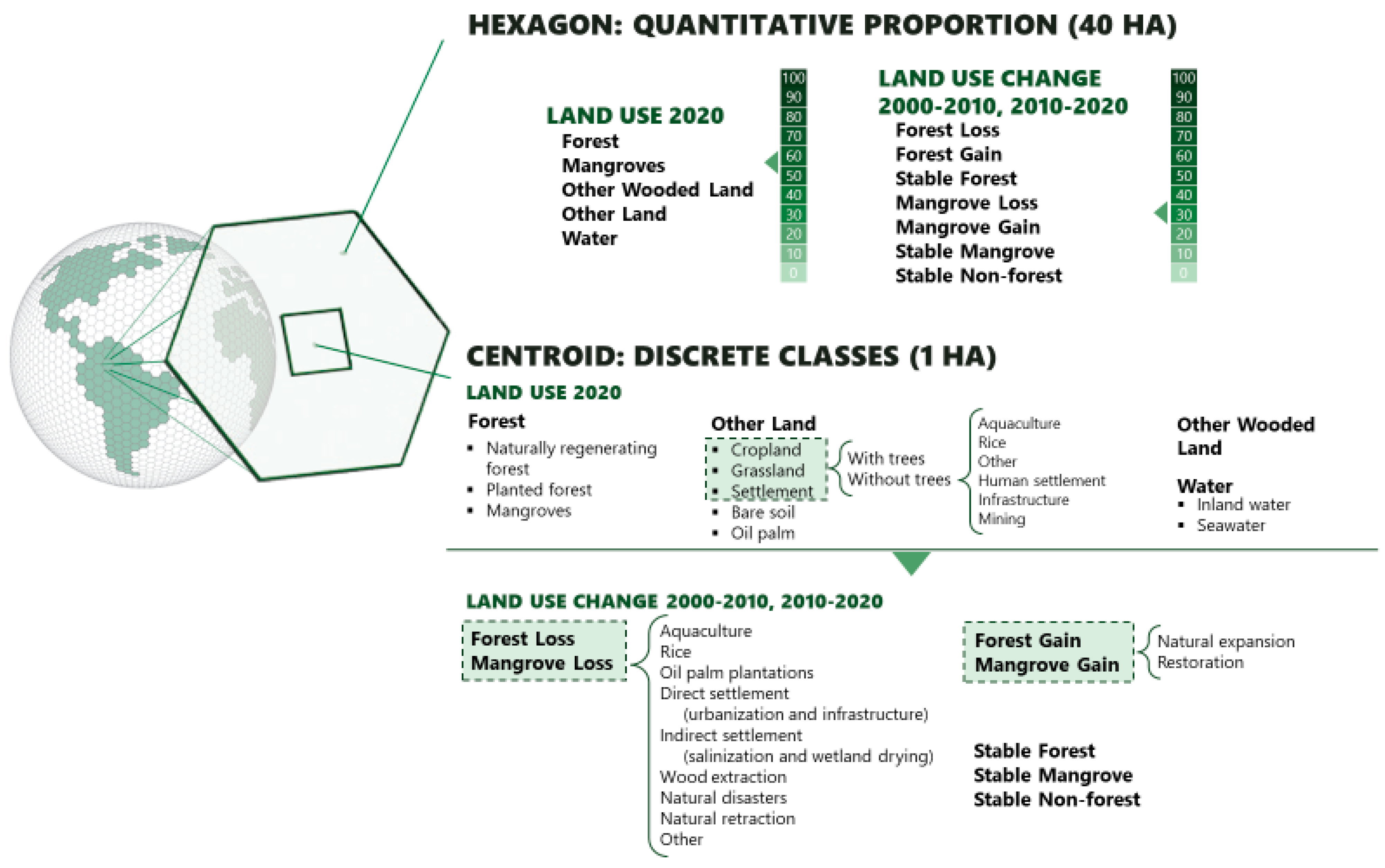
2.2. Sampling Design

Our hybrid methodology used existing remote-sensing mangrove maps for the stratification and sample allocation and local interpreters for the data collection (Figure 2). To define the strata for our sampling design, we created three key maps: a Mangrove Vegetation Index (MVI) map, a mangrove presence map and a mangrove change map. The MVI layers were produced using cloud-free Landsat 7 and Landsat 8 Tier 1 images following [16], and the band arithmetic equation MVI = (NIR − Green)/(SWIR1 − Green). Higher values of MVI in a pixel indicate a higher likelihood of mangroves being found in the pixel.

For the mangrove presence and change maps, the global mangrove mapping products used were the Global Mangrove Forest Distribution, v1 2000 [6], the Joint Research Center of the European Commission (JRC) dataset on forest cover change in tropical moist forests (TMF) 2000–2019 [17] and the Global Mangrove Watch v2 product [7] (Table S2).

First, a 600 m buffer around the Global Mangrove Watch v2 (GMW) layer was created to capture all mangrove areas off the coast. Within this buffered area, pixels from the JRC mangrove dataset and the Global Mangrove Forest Distribution v1 2000 dataset were selected. From the JRC mangrove dataset’s classes, we used the undisturbed mangroves, mangrove deforestation (2000–2019), mangrove degradation (2000–2019) and mangrove degraded or regrown before 2000 classes. From the Global Mangrove Forest Distribution v1 2000 dataset, we used the mangrove and non-mangrove pixel information for the year 2000.

This combined dataset was used to generate the two maps. The mangrove presence (stable mangrove) layer was generated using only pixels where all datasets agreed on the presence of mangroves. Pixels with disagreements between the datasets were considered the mangrove change areas. For both maps, we applied a 120 m buffer around mangroves and changed pixels to ensure we captured all mangroves and changes.

Once we defined our strata, we created our sampling frame. As the basis, we used a tessellation of the Earth’s surface into equal area hexagons (39.62 hectares each), originating from a discrete global grid of equally sized hexagons (shared with the FRA 2020 RSS; [18]). Each hexagon contains a 1-hectare square centroid to collect more detailed information on land use, land use change and related drivers. All hexagons that overlapped, even partially, with the mangrove presence and mangrove change areas were selected as part of the sampling frame.

The final stratification of hexagons into stable and change classes was performed using the MVI layers for the years 2000 and 2020, along with the mangrove presence and change maps. If more than 40% of the hexagon area was covered by pixels with change, it was assigned to the “change” stratum. If between 5–40% of the hexagon area was change pixels, and there was a maximum of 30% of stable mangroves, it was assigned to the “minimal change” stratum. If the hexagon area included less than 5% change, less than 10% stable mangrove, and the MVI indices for 2000 and 2020 were less than 4.5, it was assigned to the “no change, no forest” stratum. Finally, hexagons meeting the following criteria were assigned to the “no change forest” stratum: less than 40% of the hexagon area covered by change pixels and more than 10% covered by stable pixels, or between 5–40% coverage with change pixels, but more than 30% stable pixels, or less than 5% change coverage, more than 10% stable mangrove coverage and the 2000 MVI is greater than 4.5, or less than 5% change, less than 10% stable mangrove and the 2020 MVI is higher than 4.5.

We used stratified random sampling to select samples from each stratum (Table S2). A total of 20,900 samples were collected, with more samples collected from strata with larger areas and from the mangrove change strata [18]. All the computations to compile the maps were performed on the cloud-based platform Google Earth Engine (GEE) [19], and the random stratified sample selection was performed in Excel [20].

2.3. Data Collection and Validation

Local mangrove experts classified 20,954 samples. Experts were drawn from the FAO-FRA Remote Sensing network. When local experts were not available, experts from FAO performed the classification. Visual interpretation of the samples was completed using Collect Earth Online (CEO), a free and open-source cloud platform for viewing and interpreting high-resolution satellite imagery [12].

The assessment of mangroves in 2020 was completed based on Sentinel-2 cloud-free composite mosaics to ensure the consistency of the results globally. Land use changes were assessed using Landsat mosaics from 2000, 2010, 2018 and 2020. Very high-resolution images, freely available from Google Earth and Bing Maps, were used as auxiliary data to facilitate the understanding and classification of the samples.

Each sample had two levels of analysis: discrete classes at the centroid level (1 ha- square) and quantitative estimation of each class at the hexagon level (39.6 ha), see Figure 3. The main land use classes used in this mangrove assessment are structured according to the terms and definitions used in [21] (Appendix A). The mangrove-specific classes for land use, land-use change and deforestation drivers are based on a review of the relevant literature [22,23,24].

2.4. Data Analysis

Three time periods were collected to facilitate other analyses (2000–2010, 2010–2018 and 2018–2020). For this paper, to facilitate comparison with other research, we combined the raw data at the plot level prior to any downstream analyses to examine changes only between 2000–2010, 2010–2020 and 2000–2020. As a result, our numbers will slightly differ from those in the FAO FRA Mangrove report [25].

All land use and land use change variables were first put in terms of percentages at the unit of analysis scale (hexagon or centroid) prior to being scaled up to the subregional level (Table S3). For data derived from the hexagons, where data were collected as a percentage of the hexagon area, the mean percentage of each variable across sample plots was calculated for each stratum (e.g., % of Mangrove Loss). For data derived from the centroids, the percentage of the centroid with that land use or land use change was calculated. Then, for both hexagons and centroids, the area for the stratum was calculated by multiplying the percentage value for each land use or land use change variable by the total area of the plots in the stratum. These areas were then summed within each subregion. Variances were calculated based on these estimators using the formulas found in Table S3.

Area data estimated at the hexagon level were more precise than the centroid level. Thus, estimates of drivers collected at the centroid level were calibrated by multiplying the area of the specific change by the ratio of the area of the total change in hexagons to centroids.

3. Results

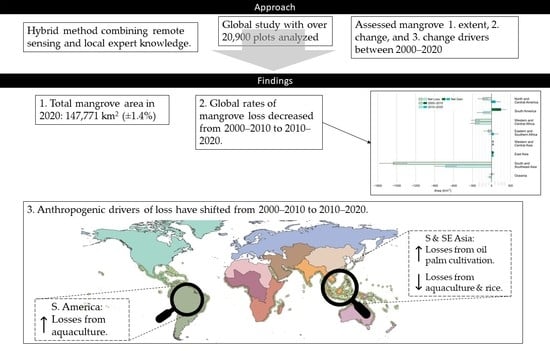
3.1. Mangrove Extent in 2020

This study found that the total area of mangroves globally in 2020 was 147,771 km² (±1.4%). The largest share was in South and Southeast Asia (44%), with smaller areas found in South America (14.5%), Western and Central Africa (14.2%), North and Central America (12.5%) and Oceania (9.9%;

Table 1. Area and 95% confidence interval of mangroves in 2020 globally and broken down by subregion.

Subregion	Mangrove Area (km2)	± (km2)	± (%)
North and Central America	18,455	821	4.4%
South America	21,400	727	3.4%
Western and Central Africa	20,926	795	3.8%
Eastern and Southern Africa	7264	493	6.8%
Western and Central Asia	209	95	45.6%
East Asia	150	52	34.7%
South and Southeast Asia	64,755	1313	2.0%
Oceania	14,611	703	4.8%
World Total	147,771	2075	1.4%

).

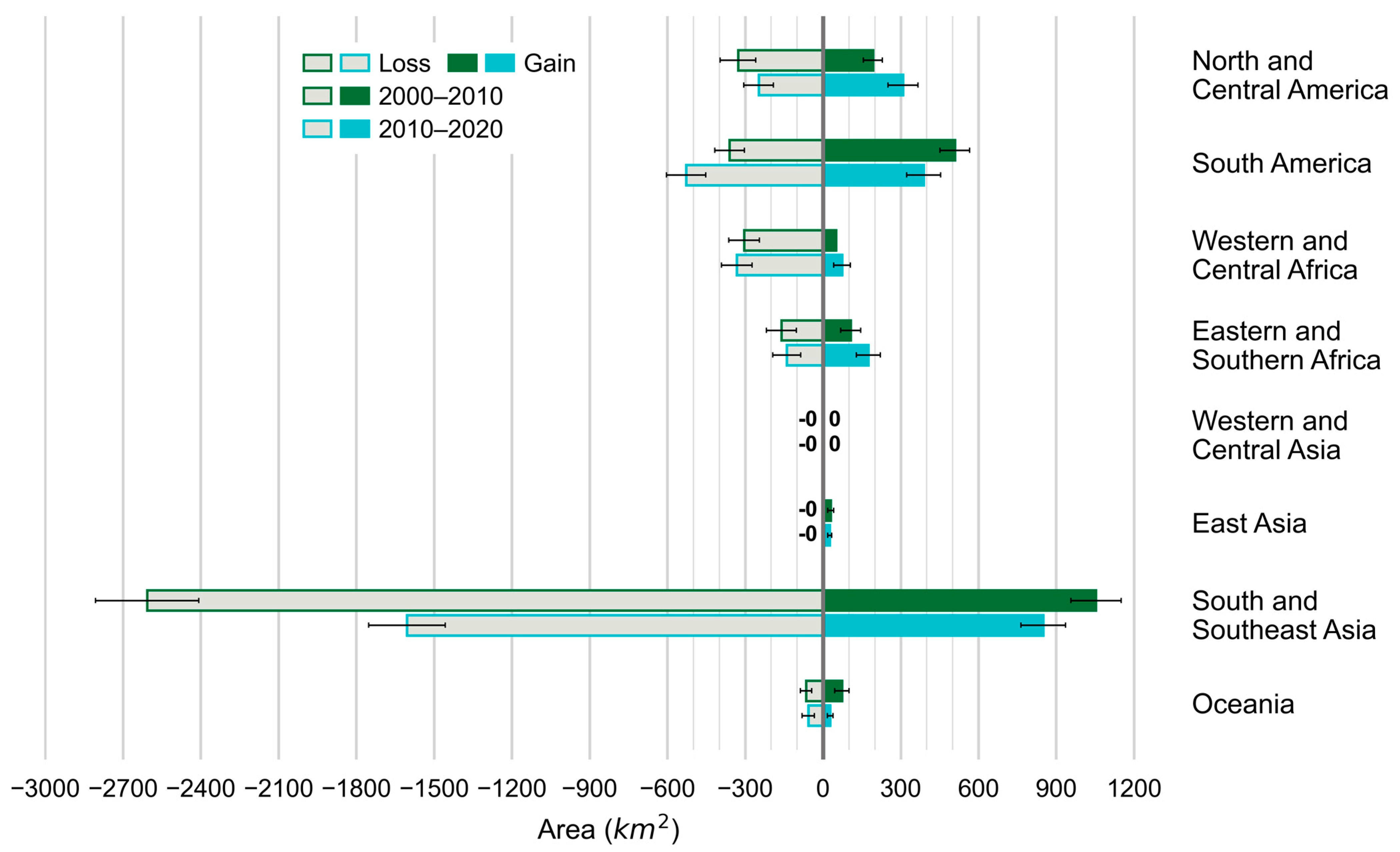
3.2. Mangrove Change 2000–2020

Overall, we observed a global trend, which shows a decrease in the net rate of mangrove deforestation over the last 20 years. While global net change remains negative, the rate of decline decreases from 1815 km² lost between 2000–2010 to 1067 km² lost between 2010–2020.

However, these global trends mask important differences between subregions (Figure 4). In South and Southeast Asia, mangrove losses have almost halved between the first and second decades. This is globally impactful, as most of the world’s mangroves by area are located in this region. North and Central America and Eastern and Southern Africa also saw improvements, moving from net losses to net gains in mangrove areas. Conversely, South America and Oceania all saw increased rates of mangrove loss. Western and Central Asia, Western and Central Africa and East Asia showed small or no difference in the rate of change.

Disaggregating net change to look at losses and gains separately, around half of the total 6314 km² mangroves lost have been offset by the establishment of 3475 km² of new mangroves. Global losses decrease by 25% between the first and the second decade of the study period. Global gains show a smaller decrease of 8.3%.

Examining subregional changes, we can identify trends behind differences in net change (Figure 5). South and Southeast Asia saw declines in the rate of both mangrove gain and mangrove loss, with a greater magnitude of change in the rate of mangrove loss leading to a net decrease in the rate of mangrove loss. North and Central America and Eastern and Southern Africa both saw decreased rates of mangrove loss and increased rates of mangrove gains, leading to a net increase in mangrove gain. Conversely, South America and Western and Central Africa both saw increased rates of mangrove loss and decreased rates of mangrove gain, leading to a net increase in mangrove loss between the two decades. However, Oceania’s observed net increase in mangrove loss can be attributed to the decreased rate of mangrove gain instead of any change in the rate of mangrove loss.

3.3. Drivers of Mangrove Loss and Gain

Globally, we found that the most prominent anthropogenic driver of mangrove loss is conversion to aquaculture (Figure 6 and Figure 7). When comparing the first decade of this study with the second, the contribution of aquaculture, direct settlement and rice cultivation notably decreased, while the contribution of indirect settlement, oil palm cultivation and other drivers notably increased. The “Other” category includes other forms of agriculture and conversion to Grasslands for livestock grazing. Breaking down the sources of anthropogenic mangrove gain by subregion shows that there are some large contributions from artificial restoration in South and Southeast Asia and Eastern and Southern Africa.

Globally, natural retraction is the largest biophysical driver of mangrove loss, and natural expansion is the largest driver of mangrove gain in both decades (Figure 6 and Figure 8). While the net global mangrove change was negative over the study period, we found that areas of natural expansion far surpassed areas lost to natural retraction and natural disasters. The natural expansion is 158% of the area of natural losses between 2000 and 2010 and 170% of natural losses between 2010 and 2020. Across both decades, this represents an area of expansion of 2968 km² compared with an area of retraction of 1812 km².

We found differences in the area estimates calculated from the hexagons and the centroids. However, the uncertainty of estimates from centroids is larger than that from the hexagons, which supported our use of the calibration procedure (Supplementary Materials).

4. Discussion

4.1. Estimates of Mangrove Extent

At the global level, there have been several attempts at mapping mangrove extent and mangrove area change [6,8,10,17,23,26]. Our estimate of 147,771 km² (±1.4%) of mangroves globally in 2020 is in line with other available estimates and is particularly close to the GMW mangrove cover estimate [8] (

Table 2. Mangrove area estimates by FAO Subregion according to different global mangrove maps. Areas for the JRC and ESA products calculated using a pixel-counting approach for the digital product. Only studies with estimates for 2020 are included in the table.

Subregion	JRC (2021, km2)	ESA (2020, km2)	GMW 3.0 (2020, km2)	This Paper (2020, km2)
East Asia	2	247	228	150
Eastern and Southern Africa	4189	9155	7917	7264
North and Central America	14,432	27,961	22,827	18,455
Oceania	11,900	20,920	16,518	14,611
South America	19,538	23,966	20,378	21,400
South and Southeast Asia	52,504	74,009	57,772	64,755
Western and Central Africa	19,849	25,004	21,428	20,926
Western and Central Asia	0	379	285	209
Total	122,414	181,639	147,352	147,771

).

Similarly, our finding that global mangrove deforestation has slowed in the past 20 years agrees with previous research [8,10]. However, slightly more of the global mangrove losses were offset by the establishment of new mangrove areas (

Table 3. Estimates of total and annual mangrove loss and gain from multiple global studies. Confidence intervals included where studies calculated them. Due to differences in study length, annual loss and gain estimates may be the most accurate for comparison. Due to differences in how geographical subdivisions were made, we compared global estimates. NA indicates that the estimate was not calculated in the study. Adapted from [8].

Study	Period	Loss in Period (km2)			Annual Loss (km2)	Gain (km2)			Annual Gain (km2)
		Est.	Lower CI	Upper CI		Est.	Lower CI	Upper CI
Hamilton and Casey 2016 [23]	2000–2012	1646	NA	NA	−137	NA	NA	NA	NA
Goldberg et al. 2020 [2]	2000–2016	−3363	NA	NA	−210	NA	NA	NA	NA
Murray et al. 2022 [10]	1999–2019	−5561	−6827	−3326	−278	1828	932	2960	91
GMW v3.0 [8]	1996–2020	−9348	−15,825	−5568	−390	4130	2238	7012	171
FRA Mangrove RSS (This Study)	2000–2020	−6314	−6923	−5706	−316	3475	3093	3857	174

). Confidence intervals varied considerably between studies (e.g., compare this study with [8,10]). Confidence intervals were not calculated for other studies due to methodological limitations [2,23].

4.2. Anthropogenic Drivers of Mangrove Loss and Gain

Previous studies have used remote sensing imagery and sophisticated machine learning approaches to identify and categorise different types of change in mangrove forests [2,11]. However, these approaches have limitations, including the similarity in spectral signatures that different land use classes present and reliance on existing datasets which can propagate error. This is the only global study of land use change leveraging local experts instead of models.

Using visual interpretation of satellite imagery and local expertise allowed us to use the surrounding landscape context and location-specific knowledge to identify multiple difficult-to-classify plots correctly. For example, during data collection, we found instances where some mangrove wood was harvested in a sustainable way, and it was still classified as stable mangrove, whereas the same sample could have been classified as mangrove loss using only satellite imagery. Further, while some anthropogenic and biophysical drivers have similar spectral signatures, we were able to distinguish between these, allowing us to distinguish between these.

Despite these different approaches, our results agreed with the earlier findings that the majority of total global mangrove loss was concentrated in the South and Southeast Asia region [2,11,23], and the key drivers were anthropogenic [2,11,22]. Broadly, we found that 72% of losses between 2000 and 2020—75% in the first decade and 68% in the second decade—were the result of human impacts. This was higher than Goldberg et al.’s (2020) [2] estimate, which found that 62% of mangrove loss was due to anthropogenic drivers using remote sensing only [2]. This difference could be attributed to differences in the types of anthropogenic losses considered, as our drivers included more granularity, e.g., aquaculture, oil palm and rice vs. commodities, but could also be due to the driver classification method or methodological approach. The Goldberg et al. (2020) [2] study used a decision-tree model based on open-source datasets to assign Landsat pixels to each driver; however, due to spectral signature similarities between anthropogenic and biophysical land uses/land covers, they could have failed to correctly assign all the losses [2].

The largest of the anthropogenic drivers is conversion for the production of agricultural commodities, including aquaculture, oil palm and rice. We found that these accounted for 44.5% of the global mangrove losses between 2000 and 2020; Goldberg et al. (2020) [2] found that these same commodities accounted for 47 per cent of mangrove losses between 2000 and 2016 [2]. Overall, we anticipate that while the rate of loss has slowed over the past 20 years, agriculture will remain the predominant anthropogenic driver of mangrove losses globally.

However, this global pattern hides some important regional differences. For example, declines in the rate of loss due to aquaculture are driven by reductions in South and Southeast Asia. In this region, the overall rate of net loss declined in the past 10 years due to growing awareness of the importance of mangroves for climate mitigation and adaptation, as well as for biodiversity, fisheries and livelihoods [27]. Other positive factors in this region include efforts to restore mangroves by governments and communities, improved regulation of the use and conversion of mangroves and increasing the area of mangroves under protection [28]. Yet, while conversion for aquaculture declined, conversion to oil palm in South and Southeast Asia sharply increased between the first and second decade of this study, as anticipated by Richards and Friess (2016) [22]. In comparison, in North and Central America, South America and Western and Central Africa, mangrove conversion to aquaculture sharply increased, indicating that better management of this driver will be needed to ensure a suitable combination of conservation and maintenance of local livelihoods [24,29].

In Western and Central Africa, the subregion with the highest rate of mangrove loss in 2010–2020, drivers of mangrove deforestation have shifted considerably in the last two decades from direct settlement to indirect settlement and agriculture. In the coming years, mangroves could continue to be threatened in this subregion by conversion to aquaculture and other forms of agriculture, natural retraction and indirect settlement, as large areas of mangroves (69%) remain unprotected [1]. Overall, anthropogenic pressure is still the most relevant through shrimp farming in South and Southeast Asia, while drivers in Africa seem closely connected to increasing demographic pressure in the region [30,31].

4.3. Biophysical Drivers of Mangrove Loss and Gain

Natural retraction due to shoreline erosion and extreme weather events was an important driver of mangrove loss observed in all sub-regions, in line with other research [2,11]. Yet, natural expansion was also an important driver of mangrove gain and mangrove retreat and regrowth were commonly observed simultaneously (see also [11]).

Moreover, the area of natural expansion was much greater than natural retraction. Given the impacts of global climate change on mangroves, including sea level rise; increases in atmospheric CO₂; rise in temperature; changes in rainfall; and a predicted increase in the frequency and severity of extreme weather, we might expect that natural retraction would outpace natural expansion [32]. Other researchers have suggested that climate change will impact different regions in different ways, likely increasing mangrove growth in areas with increased precipitation and warming and decreasing it in areas with sea level rise, increased cyclonic activity or where precipitation decreases [33,34,35,36]. Yet, where the effect sizes have been estimated, the negative impacts are much greater [35].

However, our results found the opposite trend, highlighting the difficulty in predicting the influence of global climate change on mangrove communities, given the complex interplay between local biophysical conditions and the consequences of global warming [37]. Other possible explanations include that humans are changing places where mangroves can naturally retract, e.g., by sediment removal, and the resilience of mangroves in responding to environmental changes and rapidly colonising suitable habitats when propagules are available (e.g., [38]).

4.4. Methodological Strengths, Tradeoffs and Lessons Learned

This hybrid methodology fills a gap in the literature and provides improved resolution for both anthropogenic and biophysical drivers of mangrove loss and gain while matching existing estimates of global mangrove areas and rates of change. The two broad types of approaches for evaluating mangroves—existing approaches using machine learning and our hybrid approach—each have different strengths and weaknesses and roles to play in mangrove conservation policy.

Many recent studies have leveraged advancements in automatic classification algorithms, freely available satellite imagery and the ease of cloud computation to produce maps of regional and global mangrove extent using automatic and semi-automatic classification, e.g., [10,17]. These approaches allow for wall-to-wall mapping and manually collected verification data, area estimates and confidence intervals.

Yet, distinguishing land use and between specific drivers requires additional datasets, and there are limitations imposed both by the sensor characteristics of the imagery used, persistent cloud cover and machine learning methods [2,8,39]. Further, area estimates obtained with these methods may have omission and commission errors introduced using additional data layers [2]. Many maps do not provide error analyses or confidence intervals to users, making them less useful for decision-making [40].

Our approach allows for improved resolution of drivers using a network of people knowledgeable about the local environment. The approach is robust, and local experts were able to classify samples even with high cloud cover and differentiate between different land use and land use change dynamics, including those that cannot be discriminated between using remote sensing-only approaches, e.g., [2]. Using Collect Earth Online (CEO) allowed for rapid data collection as the cloud platform is easy to use and teach to remote users in a short period of time. The use of the CEO platform allowed data collection to proceed quickly with an easy-to-use interface and our simple questionnaire that could be remotely taught in a half-day webinar. The approach is technically straightforward, requiring only basic remote sensing knowledge for the data collection and standard area estimation techniques for obtaining uncertainty with confidence intervals around land use change drivers, e.g., [41]. While no maps are produced, this approach is flexible, and it is possible to increase sampling density where additional granularity is required, such as at the country scale. In addition, the approach is repeatable, and organisations can replicate this assessment periodically, using the same network of local interpreters to maintain consistency.

This work involved 48 interpreters from all around the world, recruited from a previously established global network of remote sensing experts [18]. Organising this data collection effort was challenged by the ongoing COVID-19 pandemic in 2020 and 2021, as in-person workshops could not be held. While contact had already been established with most of the interpreters during past in-person workshops, it has sometimes been difficult to follow up with them and obtain quick results due to the remote-working modality. In addition, conversations about different land use dynamics occurring in different parts of the world emerged from the remote workshops. These discussions made it clear that local knowledge of the landscape is essential. They also reinforced the opinion that at least part of a data collection process of this type should be live, to better facilitate these emergent discussions and achieve better results.

During this data collection effort, we also learned some lessons regarding the sample plots. First, the interpretation of the hexagons using 10% area intervals was very successful. These were visually assessed by the interpreters, often without the use of a ruler. This approach was much faster than having many sample points within the plot (e.g., 100 evenly spaced grid points) and was just as accurate. In fact, after 5–6 days of data collection, the interpreters were very accurate, and an internal check found that these visual estimates were very close to estimates obtained by precisely measuring using the ruler tool in Google Earth. To ensure and improve accuracy, we used exercises ahead of data collection to become accustomed to estimating the hexagon’s area visually.

Additionally, combining the easy classification of the centroids with the more precise area estimates from the hexagons was a good approach. This approach requires benchmarking the centroid estimates of driver loss and gain with the hexagon estimates of loss and gain. The approach was successful at engaging local experts, as classifying driver loss and gain across the entire hexagon is too large of an effort. However, only using the centroids loses precision, something we have also found with using small plots of half a hectare [42].

Employing robust QAQC protocols was also important. To reduce bias in our area estimates as much as possible, we used the same definition for mangrove, mangrove change and mangrove drivers globally and employed quality control after the data collection. In addition, due to resource constraints and COVID-19 travel limitations, it was more difficult to engage interpreters for some areas of the world who were highly knowledgeable about all different types of mangrove ecosystems, requiring robust QAQC protocols. This shows how essential it is to involve local interpreters to obtain correct land use classifications.

From a policy standpoint, FAO is especially interested in reporting on land use and land use change in forestry, instead of land cover, to support countries in their assessment and monitoring of forest resources. Understanding forest resources and their changes is key to national and international environmental and developmental policy processes and is required by many international commitments, including the Paris Agreement of the United Nations Framework Convention on Climate Change (UNFCCC), the Kunming-Montreal Global Biodiversity Framework of the Convention on Biological Diversity (CBD), the United Nations Convention to Combat Desertification (UNCCD), the United Nations Strategic Plan for Forests 2030 and the Sustainable Development Goals of the Agenda 2030 (SDGs; [43]).

5. Conclusions

Using remote sensing and the knowledge of local specialists, we devised a reliable and repeatable technique. This approach was successfully used to collect data on mangrove areas in 2020, mangrove area changes between 2000 and 2020 and, most importantly, both anthropogenic and biophysical drivers of mangrove change for these periods. This is the first global study that provides information on land use based on direct interpretation of satellite imagery and not land cover for those variables, a result which was only possible with the involvement of local experts.

In line with previous estimates, our results found that globally there were 147,771 km² (±1.4%) of mangroves in 2020 and that the rate of mangrove loss has decreased between 2000–2010 and 2010 to 2020, largely driven by decreasing rates of loss in South and Southeast Asia. The contribution of different anthropogenic and biophysical drivers of loss and gain during these periods has shifted considerably. For anthropogenic drivers, aquaculture is an emerging concern in South America and Western and Central Africa, and oil palm cultivation is an emerging concern in South and Southeast Asia. For biophysical drivers, natural expansion continues to be larger than natural retraction and natural disasters combined.

Areas of future research to be considered start with deepening the analysis of the drivers. This includes collecting data on mangrove degradation, a parameter difficult to map using remote sensing but which could be addressed with sample-based interpretation by human interpreters. Our land use change drivers had relatively broad confidence intervals, so increasing the number of samples would reduce the confidence intervals for the drivers’ estimates.

Another opportunity that our sampling-based methodology offers is the intensification at a national or sub-national level to assess changes and trends in mangroves and obtain better mangrove statistics for a particular country’s national inventory [44]. FAO is already collaborating with some countries, such as Indonesia and Cuba, to use this methodology to possibly integrate the new data in their own national forest inventories. The resulting area estimates can be used to report to international conventions and processes.

Finally, there is a need for a robust global drivers database for mangrove deforestation [45] that is periodically updated. Our future assessments will focus on collecting data about drivers of loss and gain using this hybrid methodology.

References

1. Leal, M.; Spalding, M.D. (Eds.) The State of the World’s Mangroves; Global Mangrove Alliance: Washington, DC, USA, 2022. [Google Scholar]
2. Goldberg, L.; Lagomasino, D.; Thomas, N.; Fatoyinbo, T. Global declines in human-driven mangrove loss. Glob. Change Biol. 2020, 26, 5844–5855. [Google Scholar] [CrossRef] [PubMed]
3. Taillardat, P.; Friess, D.A.; Lupascu, M. Mangrove blue carbon strategies for climate change mitigation are most effective at the national scale. Biol Lett. 2018, 14, 20180251. [Google Scholar] [CrossRef] [PubMed] [Green Version]
4. Romañach, S.; Deangelis, D.; Koh, H.; Li, Y.; Teh, S.; Sulaiman, R.; Lu, Z. Conservation and restoration of mangroves: Global status, perspectives, and prognosis. Ocean. Coast. Manag. 2018, 154, 72–82. [Google Scholar] [CrossRef]
5. Hagger, V.; Worthington, T.A.; Lovelock, C.E.; Adame, M.F.; Amano, T.; Brown, M.B.; Friess, D.A.; Landis, E.; Mumby, P.J.; Morrison, T.H.; et al. Drivers of global mangrove loss and gain in social-ecological systems. Nat. Commun. 2022, 13, 6373. [Google Scholar] [CrossRef]
6. Giri, C.E.; Ochieng, L.; Tieszen, L.; Zhu, Z.; Singh, A.; Loveland, T.; Masek, J.; Duke, N. Status and distribution of mangrove forests of the world using earth observation satellite data. Glob. Ecol. Biogeogr. 2011, 20, 154–159. [Google Scholar] [CrossRef]
7. Bunting, P.; Rosenqvist, A.; Lucas, R.; Rebelo, L.-M.; Hilarides, L.; Thomas, N.; Hardy, A.; Itoh, T.; Shimada, M.; Finlayson, M. The Global Mangrove Watch—A New 2010 Global Baseline of Mangrove Extent. Remote Sens. 2018, 10, 1669. [Google Scholar] [CrossRef] [Green Version]
8. Bunting, P.; Rosenqvist, A.; Hilarides, L.; Lucas, R.M.; Thomas, N.; Tadono, T.; Worthington, T.A.; Spaldingg, M.; Murray, N.J.; Rebelo, L.M. Global mangrove extent change 1996–2020: Global Mangrove Watch version 3.0. Remote Sens. 2022, 14, 3657. [Google Scholar] [CrossRef]
9. Friess, D.A.; Rogers, K.; Lovelock, C.E.; Krauss, K.W.; Hamilton, S.E.; Lee, S.Y.; Lucas, R.; Primavera, J.; Rajkaran, A.; Shi, S. The state of the world’s mangrove forests: Past, present, and future. Annu. Rev. Environ. Resour. 2019, 44, 89–115. [Google Scholar] [CrossRef] [Green Version]
10. Murray, N.; Worthington, T.A.; Bunting, P.; Duce, S.; Hagger, V.; Lovelock, C.E.; Lucas, R.; Saunders, M.I.; Sheaves, M.; Spalding, M.; et al. High-resolution mapping of losses and gains of Earth’s tidal wetlands. Science 2022, 376, 744–749. [Google Scholar] [CrossRef]
11. Thomas, N.; Lucas, R.; Bunting, P.; Hardy, A.; Rosenqvist, A.; Simard, M. Distribution and drivers of global mangrove forest change, 1996–2010. PLoS ONE 2017, 12, e0179302. [Google Scholar] [CrossRef] [Green Version]
12. Saah, D.; Johnson, G.; Ashmall, B.; Tondapu, G.; Tenneson, K.; Patterson, M.; Poortinga, A.; Markert, K.; Quyen, N.H.; San Aung, K.; et al. Collect Earth: An online tool for systematic reference data collection in land cover and use applications. Environ. Model. Softw. 2019, 118, 166–171. [Google Scholar] [CrossRef]
13. FAO. The World’s Mangroves 1980–2005; FAO Forestry Paper 153; FAO: Rome, Italy, 2007. [Google Scholar]
14. Tomlinson, P.B. The Botany of Mangroves; Cambridge University Press: Cambridge, UK, 1986. [Google Scholar]
15. FAO. Global Forest Resources Assessment 2020; FAO: Rome, Italy, 2020. [Google Scholar]
16. Baloloy, A.B.; Blanco, A.C.; Rhommel, R.; Ana, C.S.; Nadaoka, K. Development and application of a new mangrove vegetation index (MVI) for rapid and accurate mangrove mapping. ISPRS J. Photogramm. Remote Sens. 2020, 166, 95–117. [Google Scholar] [CrossRef]
17. Vancutsem, C.; Achard, F.; Pekel, J.-F.; Vieilledent, G.; Carboni, S.; Simonetti, D.; Gallego, J.; Aragão, L.E.O.C.; Nasi, R. Long-term (1990–2019) monitoring of forest cover changes in the humid tropics. Sci. Adv. 2021, 7, eabe1603. [Google Scholar] [CrossRef]
18. FAO. FRA 2020 Remote Sensing Survey; FAO Forestry Paper No. 186; FAO: Rome, Italy, 2022. [Google Scholar] [CrossRef]
19. Gorelick, N.; Hancher, M.; Dixon, M.; Ilyushchenko, S.; Thau, D.; Moore, R. Google Earth Engine: Planetary-scale geospatial analysis for everyone. Remote Sens. Environ. 2017, 202, 18–27. [Google Scholar] [CrossRef]
20. Microsoft Corporation. Microsoft Excel. Available online: https://office.microsoft.com/excel (accessed on 30 July 2023).
21. FAO. Terms and Definitions-FRA 2020; Forest Resources Assessment Working Paper 188; FAO: Rome, Italy, 2018; Available online: www.fao.org/3/I8661EN/i8661en.pdf (accessed on 1 August 2023).
22. Richards, D.R.; Friess, D.A. Rates and drivers of mangrove deforestation in Southeast Asia, 2000–2012. Proc. Natl. Acad. Sci. USA 2016, 113, 344–349. [Google Scholar] [CrossRef] [PubMed]
23. Hamilton, S.E.; Casey, D. Creation of a high spatio-temporal resolution global database of continuous mangrove forest cover for the 21st century (CGMFC-21). Glob. Ecol. Biogeogr. 2016, 25, 729–738. [Google Scholar] [CrossRef]
24. Feka, N.Z.; Ajonina, G.N. Drivers causing decline of mangrove in West-Central Africa: A review. Int. J. Biodivers. Sci. Ecosyst. Serv. Manag. 2011, 7, 217–230. [Google Scholar] [CrossRef]
25. FAO. The World’s Mangroves 2000–2020; Forest Resources Assessment Working Paper; FAO: Rome, Italy, 2023; in press. [Google Scholar]
26. Zanaga, D.; Van De Kerchove, R.; De Keersmaecker, W.; Souverijns, N.; Brockmann, C.; Quast, R.; Wevers, J.; Grosu, A.; Paccini, A.; Vergnaud, S.; et al. ESA WorldCover 10 m 2020 v100. 2021. Available online: https://zenodo.org/record/5571936 (accessed on 1 August 2023).
27. Gerona-Daga, M.E.B.; Salmo, S.G., III. A systematic review of mangrove restoration studies in Southeast Asia: Challenges and opportunities for the United Nation’s Decade on Ecosystem Restoration. Front. Mar. Sci. 2022, 9, 987737. [Google Scholar] [CrossRef]
28. Spalding, M.; Kainuma, M.; Collins, L. World Atlas of Mangroves; Earthscan: London, UK; Washington, DC, USA, 2010. [Google Scholar]
29. de Lacerda, L.D.; Borges, R.; Ferreira, A.C. Neotropical mangroves: Conservation and sustainable use in a scenario of global climate change. Aquatic Conserv Mar Freshw Ecosyst. 2019, 29, 1347–1364. [Google Scholar] [CrossRef]
30. Duguma, L.; Bah, A.; Muthee, K.; Carsan, S.; McMullin, S.; Minang, P. Drivers and Threats Affecting Mangrove Forest Dynamics in Ghana and The Gambia. In Women Shellfishers and Food Security Project; WSFS2022_01_CRC; World Agroforestry (ICRAF): Nairobi, Kenya; Coastal Resources Center, Graduate School of Oceanography, University of Rhode Island: Narragansett, RI, USA, 2022; 53p. [Google Scholar]
31. Lontsi, F.R.Z.; Tchawa, P.; Mbaha, J.P. Mapping and Botanical Study of Pressures Causing Mangrove Dynamics of Tiko (Southwest Cameroon). Open Access Libr. J. 2023, 10, 1–19. [Google Scholar] [CrossRef]
32. CMEP. Caribbean Marine Climate Change Report Card 2017; Buckley, P., Townhill, B., Trotz, U., Nichols, K., Murray, P.A., Samuels, C.C., Gordon, A., Eds.; Commonwealth Marine Economies Programme (CMEP): London, UK, 2017; 12p. [Google Scholar]
33. Alongi, D.M. The impact of climate change on mangrove forests. Curr. Clim. Chang. Rep. 2015, 1, 30–39. [Google Scholar] [CrossRef] [Green Version]
34. Coldren, G.A.; Langley, J.A.; Feller, I.C.; Chapman, S.K. Warming accelerates mangrove expansion and surface elevation gain in a subtropical wetland. J. Ecol. 2019, 107, 79–90. [Google Scholar] [CrossRef] [Green Version]
35. Friess, D.A.; Adame, M.F.; Adams, J.B.; Lovelock, C.E. Mangrove forests under climate change in a 2 C world. Wiley Interdiscip. Rev. Clim. Change 2022, 13, 792. [Google Scholar] [CrossRef]
36. Arnaud, M.; Baird, A.J.; Morris, P.J.; Dang, T.H.; Nguyen, T.T. Sensitivity of mangrove soil organic matter decay to warming and sea level change. Glob. Chang. Biol. 2020, 26, 1899–1907. [Google Scholar] [CrossRef]
37. Bindiya, E.S.; Sreekanth, P.M.; Bhat, S.G. Conservation and Management of Mangrove Ecosystem in Diverse Perspectives. In Conservation and Sustainable Utilization of Bioresources; Springer Nature: Singapore, 2023; pp. 323–352. [Google Scholar]
38. Fickert, T. To plant or not to plant, that is the question: Reforestation vs. natural regeneration of hurricane-disturbed mangrove forests in Guanaja (Honduras). Forests 2020, 11, 1068. [Google Scholar] [CrossRef]
39. Keenan, R.J.; Reams, G.A.; Achard, F.; de Freitas, J.V.; Grainger, A.; Lindquist, E. Dynamics of global forest area: Results from the FAO Global Forest Resources Assessment 2015. For. Ecol. Manag. 2015, 352, 9–20. [Google Scholar] [CrossRef]
40. Olofsson, P.; Foody, G.M.; Stehman, S.V.; Woodcock, C.E. Making better use of accuracy data in land change studies: Estimating accuracy and area and quantifying uncertainty using stratified estimation. Remote Sens. Environ. 2013, 129, 122–131. [Google Scholar] [CrossRef]
41. Olofsson, P.; Foody, G.M.; Herold, M.; Stehman, S.V.; Woodcock, C.E.; Wulder, M.A. Good practices for estimating area and assessing accuracy of land change. Remote Sens. Environ. 2014, 148, 42–57. [Google Scholar] [CrossRef]
42. Kindgard, A.; FAO, Rome, Italy. Personal Communication, 2023.
43. FAO. Regional Technical Platform on Green Agriculture. Available online: https://www.fao.org/platforms/green-agriculture/areas-of-work/natural-resources-biodiversity-green-production/forestry/forest-and-land-use-cover-assessment-and-monitoring/en (accessed on 31 May 2023).
44. Sandker, M.; Carrillo, O.; Leng, C.; Lee, D.; d’Annunzio, R.; Fox, J. The importance of high–quality data for REDD+ monitoring and reporting. Forests 2021, 12, 99. [Google Scholar] [CrossRef]
45. Bhowmik, A.K.; Padmanaban, R.; Cabral, P.; Romeiras, M.M. Global Mangrove Deforestation and Its Interacting Social-Ecological Drivers: A Systematic Review and Synthesis. Sustainability 2022, 14, 4433. [Google Scholar] [CrossRef]
Figure 1. The global extent of mangroves. Mangrove extent from GMW v3 [8]. Subregions based on [15].
Remotesensing 15 03872 g001
Figure 2. Overview of the hybrid methodology used to assess mangroves.
Remotesensing 15 03872 g002
Figure 3. Data were collected for each plot. Modified from [18].
Remotesensing 15 03872 g003
Figure 4. Net change in mangrove area by decade and subregion. Error bars represent standard errors.
Remotesensing 15 03872 g004
Figure 5. Mangrove gain and loss by decade and subregion. Error bars represent standard errors.
Remotesensing 15 03872 g005
Figure 6. Examples of anthropogenic and biophysical drivers of mangrove loss and gain. Latest Google Satellite image refers to the latest very high-resolution image available in Google Earth for the location.
Remotesensing 15 03872 g006
Figure 7. Anthropogenic drivers of mangrove loss and gain by decade and subregion.
Remotesensing 15 03872 g007
Figure 8. Biophysical drivers of mangrove loss and gain by decade and subregion.
Remotesensing 15 03872 g008