
Landslide Susceptibility Analysis on the Vicinity of Bogotá-Villavicencio Road (Eastern Cordillera of the Colombian Andes)
 ,
,  ,
,  , , and
Abstract
:
1. Introduction
2. Materials and Methods
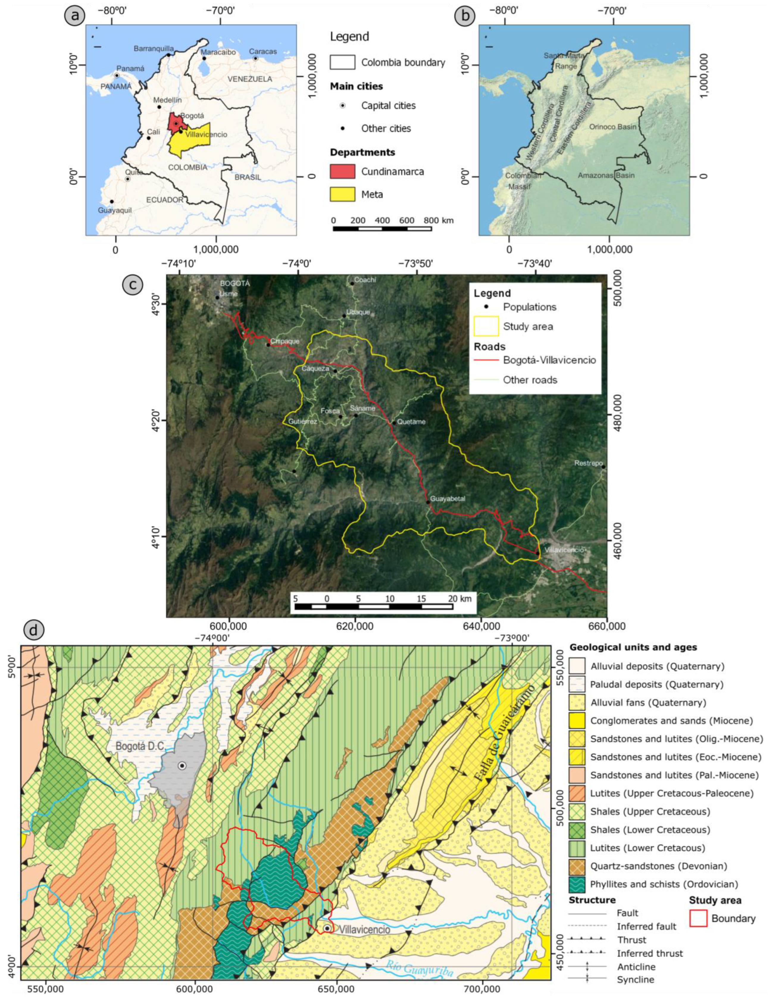
2.1. Study Area
2.2. Materials

| Information | Resources | Software |
|---|---|---|
| Digital elevation model (12.5 m resolution) | JAXA/METI ALOS PALSAR, 2011 [67,68] | Google Earth 7.3.6.9345 [72] |
| Background images | GM, GE, BM (Airbus, Maxar, Copernicus) | QGIS versión 3.18.3 [73] |
| Geology: Geological Atlas of Colombia | Layer files (shp): Servicio Geológico Colombiano, 2015 [69] | SAGA versión: 7.9.1 [74] |
| Sentinel-2 image | Copernicus, 2020 [70] | Rstudio 2022.02.2 [75] |
| Precipitation in Colombia | Raster files (tif): IDEAM, 2015 [71] |
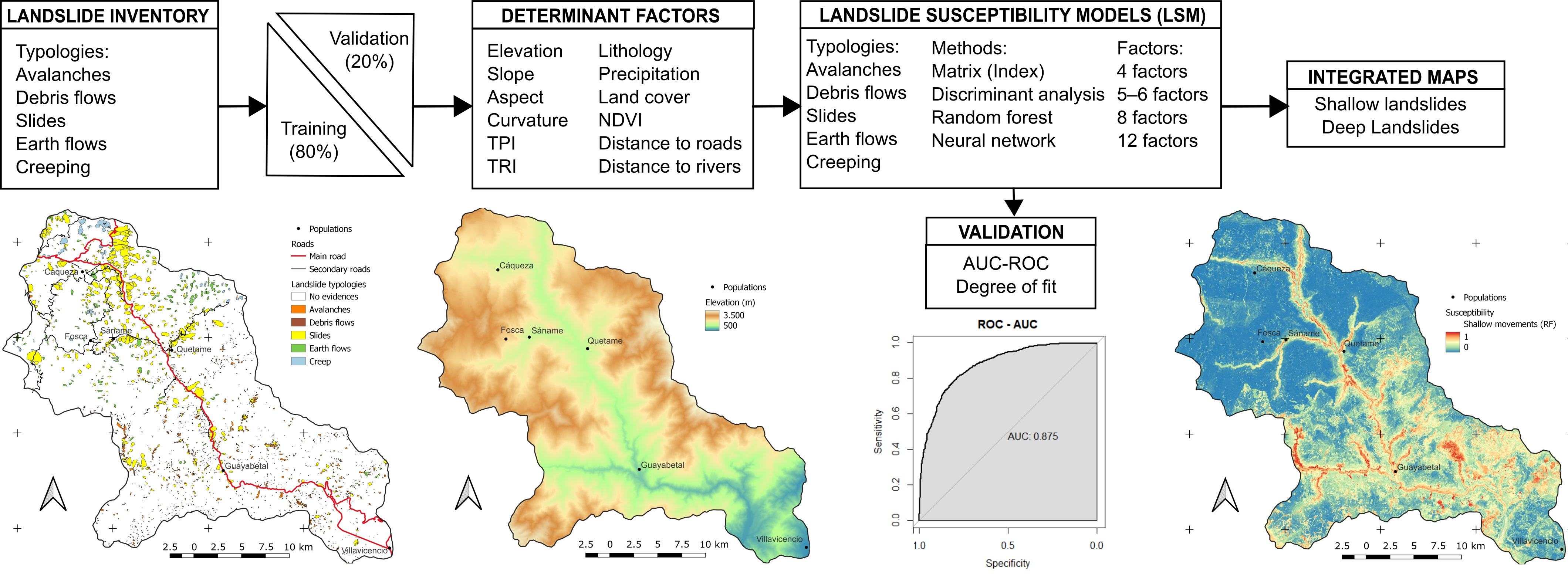
2.3. Methodology
2.3.1. Landslide Inventory
2.3.2. Analysis of Determinant Factors
2.3.3. Susceptibility Models
2.3.4. Models Validation
3. Results
3.1. Landslide Inventory
3.2. Analysis of Determinant Factors
- Avalanches show a higher density in Paleozoic quartz sandstones and phyllites, areas with scarce vegetation and NDVI between 0.1 and 0.25, altitudes between 1000 and 1500 m, slopes greater than 30°, the lower-concave sections of the hillslopes, areas with high roughness and areas near streams.
- Debris flows occur mainly in phyllites and quartz sandstones in areas with scarce vegetation, elevations above 2800 m, slopes greater than 30°, areas facing the east and southeast and areas with high roughness.
- Slides occur more frequently in Cretaceous lutites and grass-crop areas with NDVI between 0.25 and 0.4, elevations between 1500 and 1800 m, the middle-lower sections of the hillslopes and areas near streams and roads.
- Earth flows are concentrated mainly in lutites in areas with shrub vegetation with NDVI between 0.4 and 0.6, elevations between 2400 and 2800 m, slopes between 10 and 20° and the middle-lower sections of the hillslopes with low roughness.
- Creeping processes occur in lutites and grass-crop areas with NDVI between 0.25 and 0.4, elevations between 2000 and 2400 m, slopes of 0 to 10° and areas facing south with low roughness.
3.3. Susceptibility Models and Validation
4. Discussion
4.1. Lanslides Inventory
4.2. Analysis of Determinant Factors
4.3. Susceptibility Models and Validation
5. Conclusions
Author Contributions
Funding
Data Availability Statement
Acknowledgments
Conflicts of Interest
References
- Schuster, R.L. Socioeconomic significance of landslides. In Landslides: Investigation and Mitigation; Turner, A.K., Schuster, R.L., Eds.; Transportation Research Board Special Report 247; National Academy of Sciences: Washington, DC, USA, 1996; pp. 12–35. [Google Scholar]
- Petley, D.N. Global Patterns of Loss of Life from Landslides. Geology 2012, 40, 927–930. [Google Scholar] [CrossRef]
- UNDRR. Global Annual Report 2019; UNDRR: Geneva, Switzerland, 2019; Available online: https://gar.undrr.org/report-2019 (accessed on 30 May 2023).
- Guzzetti, F.; Carrara, A.; Cardinali, M.; Reichenbach, P. Landslide Hazard Evaluation: A Review of Current Techniques and Their Application in a Multi-Scale Study, Central Italy. Geomorphology 1999, 31, 181–216. [Google Scholar] [CrossRef]
- Muñoz, E.; Poveda, G.; Ochoa, A.; Caballero, H. Multifractal Analysis of Spatial and Temporal Distributions of Landslides in Colombia. In Advancing Culture of Living with Landslides; Springer International Publishing: Cham, Switzerland, 2017; pp. 1073–1079. [Google Scholar] [CrossRef]
- Aristizábal, E.; Sánchez, O. Spatial and Temporal Patterns and the Socioeconomic Impacts of Landslides in the Tropical and Mountainous Colombian Andes. Disasters 2020, 44, 596–618. [Google Scholar] [CrossRef]
- Kühnl, M.; Sapena, M.; Wurm, M.; Geiß, C.; Taubenböck, H. Multitemporal Landslide Exposure and Vulnerability Assessment in Medellín, Colombia. Nat. Hazards 2022, 1–24. [Google Scholar] [CrossRef]
- García-Delgado, H.; Petley, D.N.; Bermúdez, M.A.; Sepúlveda, S.A. Fatal Landslides in Colombia (from Historical Times to 2020) and Their Socio-Economic Impacts. Landslides 2022, 19, 1689–1716. [Google Scholar] [CrossRef]
- Gómez, D.; García, E.F.; Aristizábal, E. Spatial and Temporal Landslide Distributions Using Global and Open Landslide Databases. Nat. Hazards 2023, 117, 25–55. [Google Scholar] [CrossRef]
- CRED: EM-DAT, The International Disaster DataBase, Centre for Research on the Epidemiology of Disasters (CRED). Available online: https://www.emdat.be/ (accessed on 30 May 2023).
- UNDRR: DesInventar Sendai. Available online: https://db.desinventar.org/ (accessed on 30 May 2023).
- NASA: Open Global Landslide Catalog. Available online: https://gpm.nasa.gov/landslides/index.html (accessed on 30 May 2023).
- UN-SPIDER: Global Fatal Landslide Database (GFLD—University of Sheffield). United Nations Office for Outer Space Affairs UN-SPIDER Knowledge Portal. Available online: https://un-spider.org/links-and-resources/data-sources/global-fatal-landslide-database-gfld-university-sheffield (accessed on 30 May 2023).
- Ojeda Moncayo, J.; Donnelly, L. Landslides in Colombia and Their Impact on Towns and Cities. IAEG Pap. 2006, 112, 1–13. [Google Scholar]
- Servicio Geológico Colombiano: Sistema de Información de Movimientos en Masa—SIMMA. Available online: http://simma.sgc.gov.co/# (accessed on 30 May 2023).
- CORPES. Mapa de Amenazas Geológicas Por Remoción en Masa y Erosión del Departamento de Cundinamarca; Ingeominas: Bogotá, Colombia, 1998. [Google Scholar]
- Varnes, D.J. Landslide Hazard Zonation: A Rewiew of Principles and Practise; UNDRR: Geneva, Switzerland, 1984. [Google Scholar]
- Isaza-Restrepo, P.A.; Martínez Carvajal, H.E.; Hidalgo Montoya, C.A. Methodology for Quantitative Landslide Risk Analysis in Residential Projects. Habitat Int. 2016, 53, 403–412. [Google Scholar] [CrossRef]
- Smith, H.; Coupé, F.; Garcia-Ferrari, S.; Rivera, H.; Castro Mera, W.E. Toward Negotiated Mitigation of Landslide Risks in Informal Settlements: Reflections from a Pilot Experience in Medellín, Colombia. Ecol. Soc. 2020, 25, art19. [Google Scholar] [CrossRef]
- Ayala-García, J.; Dall’Erba, S. The Impact of Preemptive Investment on Natural Disasters. Pap. Reg. Sci. 2022, 101, 1087–1103. [Google Scholar] [CrossRef]
- García-Delgado, H.; Machuca, S.; Medina, E. Dynamic and Geomorphic Characterizations of the Mocoa Debris Flow (March 31, 2017, Putumayo Department, Southern Colombia). Landslides 2019, 16, 597–609. [Google Scholar] [CrossRef]
- Pertuz-Paz, A.; Monsalve, G.; Loaiza-Úsuga, J.C.; Caballero-Acosta, J.H.; Agudelo-Vélez, L.I.; Sidle, R.C. Linking Soil Hydrology and Creep: A Northern Andes Case. Geosciences 2020, 10, 472. [Google Scholar] [CrossRef]
- Soeters, R.; Van Westen, C.J. Slope instability recognition, analysis and zonation. In Landslides, Investigation and Mitigation; Turner, A.K., Schuster, R.L., Eds.; Transportation Research Board, National Research Council, Special Report 247; National Academy Press: Washington, DC, USA, 1996; pp. 129–177. [Google Scholar]
- Palacio Cordoba, J.; Mergili, M.; Aristizábal, E. Probabilistic Landslide Susceptibility Analysis in Tropical Mountainous Terrain Using the Physically Based r.Slope.Stability Model. Nat. Hazards Earth Syst. Sci. 2020, 20, 815–829. [Google Scholar] [CrossRef] [Green Version]
- Hidalgo, C.A.; Vega, J.A. Probabilistic Landslide Risk Assessment in Water Supply Basins: La Liboriana River Basin (Salgar-Colombia). Nat. Hazards 2021, 109, 273–301. [Google Scholar] [CrossRef]
- Marín, R.J.; Velásquez, M.F.; Sánchez, O. Applicability and Performance of Deterministic and Probabilistic Physically Based Landslide Modeling in a Data-Scarce Environment of the Colombian Andes. J. S. Am. Earth Sci. 2021, 108, 103175. [Google Scholar] [CrossRef]
- Marín, R.J.; Mattos, Á.J.; Fernández-Escobar, C.J. Understanding the Sensitivity to the Soil Properties and Rainfall Conditions of Two Physically-Based Slope Stability Models. Boletín Geol. 2022, 44, 93–109. [Google Scholar] [CrossRef]
- García-Delgado, H. The San Eduardo Landslide (Eastern Cordillera of Colombia): Reactivation of a Deep-Seated Gravitational Slope Deformation. Landslides 2020, 17, 1951–1964. [Google Scholar] [CrossRef]
- Prada-Sarmiento, L.F.; Cabrera, M.A.; Camacho, R.; Estrada, N.; Ramos-Cañón, A.M. The Mocoa Event on March 31: Analysis of a Series of Mass Movements in a Tropical Environment of the Andean-Amazonian Piedmont. Landslides 2019, 16, 2459–2468. [Google Scholar] [CrossRef]
- Cheng, D.; Cui, Y.; Su, F.; Jia, Y.; Choi, C.E. The Characteristics of the Mocoa Compound Disaster Event, Colombia. Landslides 2018, 15, 1223–1232. [Google Scholar] [CrossRef] [Green Version]
- Vargas-Cuervo, G.; Rotigliano, E.; Conoscenti, C. Prediction of Debris-Avalanches and -Flows Triggered by a Tropical Storm by Using a Stochastic Approach: An Application to the Events Occurred in Mocoa (Colombia) on 1 April 2017. Geomorphology 2019, 339, 31–43. [Google Scholar] [CrossRef]
- Braab, E.E. Innovative Approaches to Landslide Hazard and Risk Mapping. In Proceedings of the 4th International Symposium on Landslides, Toronto, ON, Canada, 16–21 September 1984; pp. 307–323. [Google Scholar]
- Reichenbach, P.; Rossi, M.; Malamud, B.D.; Mihir, M.; Guzzetti, F. A Review of Statistically-Based Landslide Susceptibility Models. Earth Sci. Rev. 2018, 180, 60–91. [Google Scholar] [CrossRef]
- Irigaray, C.; Fernández, T.; Chacón, J. Comparative Analysis of Methods for Landslide Susceptibility Mapping. In Landslides, Proceedings of the 8th International Conference and Field Trip on Landslides, Granada, Spain, 27–28 September 1996; CRC Press: Boca Raton, FL, USA; pp. 373–384.
- Irigaray, C.; Fernández, T.; El Hamdouni, R.; Chacón, J. Verification of Landslide Susceptibility Mapping: A Case Study. Earth Surf. Process. Landf. 1999, 24, 537–544. [Google Scholar]
- Fernández, T.; Irigaray, C.; El Hamdouni, R.; Chacón, J. Methodology for Landslide Susceptibility Mapping by Means of a GIS. Application to the Contraviesa Area (Granada, Spain). Nat. Hazards 2003, 30, 297–308. [Google Scholar] [CrossRef]
- Chung, C.-J.F.; Fabbri, A.G. Probabilistic Prediction Models for Landslide Hazard Mapping. Photogramm. Eng. Remote Sens. 1999, 65, 1389–1399. [Google Scholar]
- Guzzetti, F.; Reichenbach, P.; Cardinali, M.; Galli, M.; Ardizzone, F. Probabilistic Landslide Hazard Assessment at the Basin Scale. Geomorphology 2005, 72, 272–299. [Google Scholar] [CrossRef]
- Baeza, C.; Corominas, J. Assessment of Shallow Landslide Susceptibility by Means of Multivariate Statistical Techniques. Earth Surf. Process. Landf. 2001, 26, 1251–1263. [Google Scholar] [CrossRef]
- Merghadi, A.; Yunus, A.P.; Dou, J.; Whiteley, J.; ThaiPham, B.; Bui, D.T.; Avtar, R.; Abderrahmane, B. Machine Learning Methods for Landslide Susceptibility Studies: A Comparative Overview of Algorithm Performance. Earth Sci. Rev. 2020, 207, 103225. [Google Scholar] [CrossRef]
- Pradhan, B.; Lee, S. Regional Landslide Susceptibility Analysis Using Back-Propagation Neural Network Model at Cameron Highland, Malaysia. Landslides 2010, 7, 13–30. [Google Scholar] [CrossRef]
- Bui, D.T.; Tuan, T.A.; Klempe, H.; Pradhan, B.; Revhaug, I. Spatial Prediction Models for Shallow Landslide Hazards: A Comparative Assessment of the Efficacy of Support Vector Machines, Artificial Neural Networks, Kernel Logistic Regression, and Logistic Model Tree. Landslides 2016, 13, 361–378. [Google Scholar] [CrossRef]
- Pourghasemi, H.R.; Rahmati, O. Prediction of the Landslide Susceptibility: Which Algorithm, Which Precision? Catena 2018, 162, 177–192. [Google Scholar] [CrossRef]
- Salazar Gutiérrez, L.F.; Menjivar Flores, J.C.; Martínez Carvajal, H.E. Susceptibility Factors of Drainage Basins to Shallow Landslides in Coffee-Growing Areas in the Department of Caldas, Colombia. Environ. Earth Sci. 2021, 80, 145. [Google Scholar] [CrossRef]
- Goyes-Peñafiel, P.; Hernandez-Rojas, A. Landslide Susceptibility Index Based on the Integration of Logistic Regression and Weights of Evidence: A Case Study in Popayan, Colombia. Eng. Geol. 2021, 280, 105958. [Google Scholar] [CrossRef]
- Calderón-Guevara, W.; Sánchez-Silva, M.; Nitescu, B.; Villarraga, D.F. Comparative Review of Data-Driven Landslide Susceptibility Models: Case Study in the Eastern Andes Mountain Range of Colombia. Nat. Hazards 2022, 113, 1105–1132. [Google Scholar] [CrossRef]
- Aristizábal, E.; López, S.; Sánchez, O.; Vásquez, M.; Rincón, F.; Ruiz-Vásquez, D.; Restrepo, S.; Valencia, J.S. Evaluación de La Amenaza Por Movimientos En Masa Detonados Por Lluvias Para Una Región de Los Andes Colombianos Estimando La Probabilidad Espacial, Temporal, y Magnitud. Rev. Boletín Geol. 2019, 41, 85–105. [Google Scholar] [CrossRef]
- Aristizábal, E.; Morales-García, P.; Vásquez-Guarín, M.; Ruíz-Vásquez, D.; Palacio-Córdoba, J.; Ángel-Cárdenas, F.P.; Caballero-Acosta, H.; Ordóñez-Carmona, O. Metodologías Para La Evaluación de La Amenaza Por Movimientos En Masa Como Parte de Los Estudios Básico de Amenaza: Caso de Estudio Municipio de Andes, Antioquia, Colombia. Boletín Geol. 2022, 43, 199–217. [Google Scholar] [CrossRef]
- Ruiz-Vásquez, D.; Aristizábal, E. Landslide Susceptibility Assessment in Mountainous and Tropical Scarce-Data Regions Using Remote Sensing Data: A Case Study in the Colombian Andes. In EGU General Assembly; EGU: Vienna, Austria; 8–13 April 2018, p. 3408.
- Correa Muñoz, N.A.; Higidio Castro, J.F. Determination of Landslide Susceptibility in Linear Infrastructure. Case: Aqueduct Network in Palacé, Popayan (Colombia). Ing. Investig. 2017, 37, 17–24. [Google Scholar] [CrossRef]
- Pradhan, A.M.S.; Lee, J.-M.; Kim, Y.-T. Semi-Quantitative Method to Identify the Vulnerable Areas in Terms of Building Aggregation for Probable Landslide Runout at the Regional Scale: A Case Study from Soacha Province, Colombia. Bull. Eng. Geol. Environ. 2019, 78, 5745–5762. [Google Scholar] [CrossRef]
- Valencia Ortiz, J.A.; Martínez-Graña, A.M. A Neural Network Model Applied to Landslide Susceptibility Analysis (Capitanejo, Colombia). Geomat. Nat. Hazards Risk 2018, 9, 1106–1128. [Google Scholar] [CrossRef] [Green Version]
- Renza, D.; Cárdenas, E.A.; Martinez, E.; Weber, S.S. CNN-Based Model for Landslide Susceptibility Assessment from Multispectral Data. Appl. Sci. 2022, 12, 8483. [Google Scholar] [CrossRef]
- Cullen, C.A.; Al Suhili, R.; Aristizabal, E. A Landslide Numerical Factor Derived from CHIRPS for Shallow Rainfall Triggered Landslides in Colombia. Remote Sens. 2022, 14, 2239. [Google Scholar] [CrossRef]
- Aristizábal Giraldo, E.V.; García Aristizábal, E.; Marín Sánchez, R.; Gómez Cardona, F.; Guzmán Martínez, J.C. Rainfall-Intensity Effect on Landslide Hazard Assessment Due to Climate Change in North-Western Colombian Andes. Rev. Fac. Ing. Univ. Antioquia 2022, 103, 51–66. [Google Scholar] [CrossRef]
- Marín, R.J.; García, E.F.; Aristizábal, E. Effect of Basin Morphometric Parameters on Physically-Based Rainfall Thresholds for Shallow Landslides. Eng. Geol. 2020, 278, 105855. [Google Scholar] [CrossRef]
- Marín, R.J.; Velásquez, M.F.; García, E.F.; Alvioli, M.; Aristizábal, E. Assessing Two Methods of Defining Rainfall Intensity and Duration Thresholds for Shallow Landslides in Data-Scarce Catchments of the Colombian Andean Mountains. Catena 2021, 206, 105563. [Google Scholar] [CrossRef]
- Gutiérrez Alvis, D.E.; Bornachera Zarate, L.S.; Mosquera Palacios, D.J. Sistema de Alerta Temprana Por Movimiento En Masa Inducido Por Lluvia Para Ciudad Bolívar (Colombia). Ing. Solidar. 2018, 14, 26. [Google Scholar] [CrossRef] [Green Version]
- Ramos-Cañón, A.M.; Prada-Sarmiento, L.F.; Trujillo-Vela, M.G.; Macías, J.P.; Santos-R, A.C. Linear Discriminant Analysis to Describe the Relationship between Rainfall and Landslides in Bogotá, Colombia. Landslides 2016, 13, 671–681. [Google Scholar] [CrossRef]
- Velásquez, N. Assessment of Deep Convective Systems in the Colombian Andean Region. Hydrology 2022, 9, 119. [Google Scholar] [CrossRef]
- Ortega, L.C.; Cañón, J.E. Correlative Analysis of Climate Impacts in an Andean Municipality of Colombia. Rev. Cienc. Agrícolas 2022, 39, 143–159. [Google Scholar] [CrossRef]
- Parravano, V.; Teixell, A.; Mora, A. Influence of Salt in the Tectonic Development of the Frontal Thrust Belt of the Eastern Cordillera (Guatiquía Area, Colombian Andes). Interpretation 2015, 3, SAA17–SAA27. [Google Scholar] [CrossRef] [Green Version]
- Chicangana, G.; Kammer, A. Evolución Tectónica de La Cordillera Oriental de Colombia. Desde La Apertura Del Océano Iapeto Hasta la Conformación de la Pangea: Una Visión Preliminar. Primera Parte: Aspectos Geológicos. Geol. Colomb. 2013, 38, 64–74. [Google Scholar]
- Servicio Geológico Colombiano: Mapa geológico de Colombia. 2019. Available online: https://www2.sgc.gov.co/MGC/Paginas/mgc2M2019.aspx (accessed on 30 May 2023).
- DANE: Censo Nacional de Población y Vivienda. 2018. Available online: https://www.dane.gov.co/index.php/estadisticas-por-tema/demografia-y-poblacion/censo-nacional-de-poblacion-y-vivenda-2018 (accessed on 30 May 2023).
- Pulido, O.; Gómez, L.S. Geología Plancha 266 Villavicencio. In Memoria Explicativa; Ingeominas: Bogotá, Colombia, 2001. [Google Scholar]
- JAXA-METI. ALOS Systematic Observation Strategy—PALSAR. Available online: https://www.eorc.jaxa.jp/ALOS/en/obs/palsar_strat.htm (accessed on 30 May 2023).
- Alaska Satellite Facility. Available online: https://asf.alaska.edu/data-sets/sar-data-sets/alos-palsar/ (accessed on 30 May 2023).
- Servicio Geológico Colombiano. Atlas Geológico de Colombia. 2015. Available online: https://www2.sgc.gov.co/MGC/Paginas/agc_500K2015.aspx (accessed on 30 May 2023).
- Copernicus Open Access Hub. Available online: https://scihub.copernicus.eu/dhus/ (accessed on 30 May 2023).
- Ideam. Atlas Climatológico de Colombia. Available online: http://atlas.ideam.gov.co/visorAtlasClimatologico.html (accessed on 30 May 2023).
- Google Earth. Available online: https://www.google.es/intl/es/earth/index.html (accessed on 30 May 2023).
- QGIS 3. A Free and Open Source Geographic Information System. 2023. Available online: https://www.qgis.org/en/site/ (accessed on 30 May 2023).
- SAGA. System for Automated Geoscientific Analyses. Available online: https://saga-gis.sourceforge.io/en/index.html (accessed on 30 May 2023).
- Rstudio. Available online: https://www.rstudio.com/categories/rstudio-ide/ (accessed on 30 May 2023).
- Chacón, J.; Irigaray, C.; Fernández, T.; El Hamdouni, R. Engineering Geology Maps: Landslides and Geographical Information Systems. Bull. Eng. Geol. Environ. 2006, 65, 341–411. [Google Scholar] [CrossRef]
- Guzzetti, F.; Mondini, A.C.; Cardinali, M.; Fiorucci, F.; Santangelo, M.; Chang, K. Landslide Inventory Maps: New Tools for an Old Problem. Earth Sci. Rev. 2012, 112, 42–66. [Google Scholar] [CrossRef] [Green Version]
- Varnes, D.J. Slope Movements Types and Processes. In Landslides Analysis and Control; Schuster, R.L., Krizek, R.J., Eds.; National Academy of Sciences: Washington, DC, USA, 1978; pp. 11–33. [Google Scholar]
- WP/WLI; Cruden, D.M. A Suggested Method for Describing the Activity of a Landslide. Bull. Int. Assoc. Eng. Geol. 1993, 47, 53–57. [Google Scholar]
- Bravo-López, E.; Fernández Del Castillo, T.; Sellers, C.; Delgado-García, J. Analysis of Conditioning Factors in Cuenca, Ecuador, for Landslide Susceptibility Maps Generation Employing Machine Learning Methods. Land 2023, 12, 1135. [Google Scholar] [CrossRef]
- Rouse, J.; Haas, R.; Schell, J.; Deering, D. Third Earth Resources Technology Satellite. In Monitoring Vegetation Systems in the Great Plains with ERTS; Technical Presentations; NASA: Washington, DC, USA, 1974; Volume I, pp. 309–317. [Google Scholar]
- Pacheco-Quevedo, R.; Velastegui-Montoya, A.; Montalván-Burbano, N.; Morante-Carballo, F.; Korup, O.; Rennó, C.D. Land use and land cover as a conditioning factor in landslide susceptibility: A literature review. Landslides 2023, 20, 967–982. [Google Scholar] [CrossRef]
- DeGraff, J.V.; Romesburg, H.C. Regional Landslide Susceptibility Assessment for Wildland Management: A Matrix Approach. In Thresholds in Geomorphology; Coates, D.R., Vitek, J.D., Eds.; Routledge: Boston, MA, USA, 1980; pp. 401–414. [Google Scholar]
- Irigaray Fernández, C.; Fernández del Castillo, T.; El Hamdouni, R.; Chacón Montero, J. Evaluation and Validation of Landslide-Susceptibility Maps Obtained by a GIS Matrix Method: Examples from the Betic Cordillera (Southern Spain). Nat. Hazards 2007, 41, 61–79. [Google Scholar] [CrossRef]
- Li, L.; Lan, H.; Wu, Y. How Sample Size Can Effect Landslide Size Distribution. Geoenviron. Disasters 2016, 3, 18. [Google Scholar] [CrossRef] [Green Version]
- Shao, X.; Ma, S.; Xu, C.; Zhou, Q. Effects of Sampling Intensity and Non-Slide/Slide Sample Ratio on the Occurrence Probability of Coseismic Landslides. Geomorphology 2020, 363, 107222. [Google Scholar] [CrossRef]
- Huang, F.; Cao, Z.; Jiang, S.-H.; Zhou, C.; Huang, J.; Guo, Z. Landslide Susceptibility Prediction Based on a Semi-Supervised Multiple-Layer Perceptron Model. Landslides 2020, 17, 2919–2930. [Google Scholar] [CrossRef]
- Sameen, M.I.; Pradhan, B.; Bui, D.T.; Alamri, A.M. Systematic Sample Subdividing Strategy for Training Landslide Susceptibility Models. Catena 2020, 187, 104358. [Google Scholar] [CrossRef]
- Dornik, A.; Drăguţ, L.; Oguchi, T.; Hayakawa, Y.; Micu, M. Influence of Sampling Design on Landslide Susceptibility Modeling in Lithologically Heterogeneous Areas. Sci. Rep. 2022, 12, 2106. [Google Scholar] [CrossRef]
- Carrara, A. Multivariate Models for Landslide Hazard Evaluation. J. Int. Assoc. Math. Geol. 1983, 15, 403–426. [Google Scholar] [CrossRef]
- Breiman, L. Random Forests. Mach. Learn. 2001, 45, 5–32. [Google Scholar] [CrossRef] [Green Version]
- Dou, J.; Yunus, A.P.; Tien Bui, D.; Merghadi, A.; Sahana, M.; Zhu, Z.; Chen, C.-W.; Khosravi, K.; Yang, Y.; Pham, B.T. Assessment of Advanced Random Forest and Decision Tree Algorithms for Modeling Rainfall-Induced Landslide Susceptibility in the Izu-Oshima Volcanic Island, Japan. Sci. Total Environ. 2019, 662, 332–346. [Google Scholar] [CrossRef] [PubMed]
- Nefeslioglu, H.A.; Sezer, E.; Gokceoglu, C.; Bozkir, A.S.; Duman, T.Y. Assessment of Landslide Susceptibility by Decision Trees in the Metropolitan Area of Istanbul, Turkey. Math. Probl. Eng. 2010, 2010, 901095. [Google Scholar] [CrossRef] [Green Version]
- Miner, A.; Vamplew, P.; Windle, D.J.; Flentje, P.; Warner, P. A Comparative Study of Various Data Mining Techniques as Applied to the Modeling of Landslide Susceptibility on the Bellarine Peninsula, Victoria, Australia. In Geologically Active, Proceedings of the 11th IAEG Congress of the International Association of Engineering Geology and the Environment, Auckland, New Zealand, 5–10 September 2010; CRC Press: Boca Raton, FL, USA, 2010. [Google Scholar]
- Bravo-López, E.; Fernández Del Castillo, T.; Sellers, C.; Delgado-García, J. Landslide Susceptibility Mapping of Landslides with Artificial Neural Networks: Multi-Approach Analysis of Backpropagation Algorithm Applying the Neuralnet Package in Cuenca, Ecuador. Remote Sens. 2022, 14, 3495. [Google Scholar] [CrossRef]
- Ciaburro, G.; Venkateswaran, B. Neural Network with R: Smart Models Using CNN, RNN, Deep Learning, and Artificial Intelligence Principles; Packt Publishing Ltd.: Birmingham, UK, 2017; Volume 91. [Google Scholar]
- Günther, F.; Fritsch, S. Neuralnet: Training of Neural Networks. R J. 2010, 2, 30–38. [Google Scholar] [CrossRef] [Green Version]
- Zare, M.; Pourghasemi, H.R.; Vafakhah, M.; Pradhan, B. Landslide Susceptibility Mapping at Vaz Watershed (Iran) Using an Artificial Neural Network Model: A Comparison between Multilayer Perceptron (MLP) and Radial Basic Function (RBF) Algorithms. Arab. J. Geosci. 2013, 6, 2873–2888. [Google Scholar] [CrossRef]
- Pham, B.T.; Tien Bui, D.; Prakash, I.; Dholakia, M.B. Hybrid Integration of Multilayer Perceptron Neural Networks and Machine Learning Ensembles for Landslide Susceptibility Assessment at Himalayan Area (India) Using GIS. Catena 2017, 149, 52–63. [Google Scholar] [CrossRef]
- Gholamy, A.; Kreinovich, V.; Kosheleva, O. Why 70/30 or 80/20 Relation between Training and Testing Sets: A Pedagogical Explanation. Dep. Tech. Rep. 2018, 1209, 1–6. [Google Scholar]
- Vu, H.L.; Ng, K.T.W.; Richter, A.; An, C. Analysis of input set characteristics and variances on k-fold cross validation for a Recurrent Neural Network model on waste disposal rate estimation. J. Environ. Manag. 2022, 311, 114869. [Google Scholar] [CrossRef]
- Zou, K.; O’Malley, A.; Mauri, L. Receiver-Operating Characteristic Analysis for Evaluating Diagnostic Tests and Predictive Models. Circulation 2007, 115, 654–657. [Google Scholar] [CrossRef] [Green Version]
- Yilmaz, I. A Case Study from Koyulhisar (Sivas-Turkey) for Landslide Susceptibility Mapping by Artificial Neural Networks. Bull. Eng. Geol. Environ. 2009, 68, 297–306. [Google Scholar] [CrossRef]
- Park, S.; Choi, C.; Kim, B.; Kim, J. Landslide Susceptibility Mapping Using Frequency Ratio, Analytic Hierarchy Process, Logistic Regression, and Artificial Neural Network Methods at the Inje Area, Korea. Environ. Earth Sci. 2013, 68, 1443–1464. [Google Scholar] [CrossRef]
- Flórez-García, A.C.; Pérez Castillo, J.N. Técnicas Para La Predicción Espacial de Zonas Susceptibles a Deslizamientos. Av. Investig. Ing. 2019, 16, 20–48. [Google Scholar] [CrossRef] [Green Version]
- Yi, Y.; Zhang, W.; Xu, X.; Zhang, Z.; Wu, X. Evaluation of Neural Network Models for Landslide Susceptibility Assessment. Int. J. Digit. Earth 2022, 15, 934–953. [Google Scholar] [CrossRef]
- Aslam, B.; Zafar, A.; Khalil, U. Comparative Analysis of Multiple Conventional Neural Networks for Landslide Susceptibility Mapping. Nat. Hazards 2023, 115, 673–707. [Google Scholar] [CrossRef]
- Chung, C.J.F.; Fabbri, A.G. Validation of Spatial Prediction Models for Landslide Hazard Mapping. Nat. Hazards 2003, 30, 451–472. [Google Scholar] [CrossRef]
- Conforti, M.; Pascale, S.; Robustelli, G.; Sdao, F. Evaluation of Prediction Capability of the Artificial Neural Networks for Mapping Landslide Susceptibility in the Turbolo River Catchment (Northern Calabria, Italy). Catena 2014, 113, 236–250. [Google Scholar] [CrossRef]
- Hungr, O.; Leroueil, S.; Picarelli, L. The Varnes Classification of Landslide Types, an Update. Landslides 2014, 11, 167–194. [Google Scholar] [CrossRef]
- Fernández, T.; Pérez García, J.L.; Gómez López, J.M.; Cardenal, F.J.; Moya-Giménez, F.; Delgado, J. Multitemporal Landslide Inventory and Activity Analysis by Means of Aerial Photogrammetry and LiDAR Techniques in an Area of Southern Spain. Remote Sens. 2021, 13, 2110. [Google Scholar] [CrossRef]
- Gariano, S.L.; Guzzetti, F. Landslides in a Changing Climate. Earth Sci. Rev. 2016, 162, 227–252. [Google Scholar] [CrossRef] [Green Version]
- Correa, O.; García, F.; Bernal, G.; Cardona, O.D.; Rodriguez, C. Early Warning System for Rainfall-Triggered Landslides Based on Real-Time Probabilistic Hazard Assessment. Nat. Hazards 2020, 100, 345–361. [Google Scholar] [CrossRef] [Green Version]
- García-Delgado, H.; Contreras, N.M. Historical Distribution for Landslides Triggered by Earthquakes in the Colombian Region. In Proceedings of the XIII International Symposium on Landslides, Cartagena, Colombia, 15–19 June 2020. [Google Scholar]
- Bermúdez, M.A.; Velandia, F.; García-Delgado, H.; Jiménez, D.; Bernet, M. Exhumation of the Southern Transpressive Bucaramanga Fault, Eastern Cordillera of Colombia: Insights from Detrital, Quantitative Thermochronology and Geomorphology. J. S. Am. Earth Sci. 2021, 106, 103057. [Google Scholar] [CrossRef]
- Grima, N.; Edwards, D.; Edwards, F.; Petley, D.; Fisher, B. Landslides in the Andes: Forests Can Provide Cost-Effective Landslide Regulation Services. Sci. Total Environ. 2020, 745, 141128. [Google Scholar] [CrossRef] [PubMed]
- Vorpahl, P.; Elsenbeer, H.; Märker, M.; Schröder, B. How Can Statistical Models Help to Determine Driving Factors of Landslides? Ecol. Modell. 2012, 239, 27–39. [Google Scholar] [CrossRef]
- Zhu, A.-X.; Miao, Y.; Yang, L.; Bai, S.; Liu, J.; Hong, H. Comparison of the Presence-Only Method and Presence-Absence Method in Landslide Susceptibility Mapping. Catena 2018, 171, 222–233. [Google Scholar] [CrossRef]
- Costanzo, D.; Rotigliano, E.; Irigaray, C.; Jiménez-Perálvarez, J.D.; Chacón, J. Factors Selection in Landslide Susceptibility Modelling on Large Scale Following the Gis Matrix Method: Application to the River Beiro Basin (Spain). Nat. Hazards Earth Syst. Sci. 2012, 12, 327–340. [Google Scholar] [CrossRef]
- Meena, S.R.; Puliero, S.; Bhuyan, K.; Floris, M.; Catani, F. Assessing the Importance of Conditioning Factor Selection in Landslide Susceptibility for the Province of Belluno (Region of Veneto, Northeastern Italy). Nat. Hazards Earth Syst. Sci. 2022, 22, 1395–1417. [Google Scholar] [CrossRef]
- Liu, L.L.; Yang, C.; Wang, X.M. Landslide Susceptibility Assessment Using Feature Selection-Based Machine Learning Models. Geomech. Eng. 2021, 25, 1–16. [Google Scholar]
- Chacón Montero, J.; Irigaray Fernández, C.; Fernández del Castillo, T. Large to Middle Scale Landslides Inventory, Analysis and Mapping with Modelling and Assessment of Derived Susceptibility, Hazards and Risks in a GIS. In International Congress International Association of Engineering Geology; A.A. Balkema: Rotterdam, The Netherlands, 1994; pp. 4669–4678. [Google Scholar]
- van Westen, C.; van Asch, T.; Soeters, R. Landslide hazard and risk zonation—Why is it still so difficult? Bull. Eng. Geol. Environ. 2006, 65, 167–184. [Google Scholar] [CrossRef]
- Huabin, W.; Gangjun, L.; Weiya, X.; Gonghui, W. GIS-based landslide hazard assessment: An overview. Prog. Phys. Geogr. Earth Environ. 2005, 29, 548–567. [Google Scholar] [CrossRef]
- Korup, O.; Stolle, A. Landslide Prediction from Machine Learning. Geol. Today 2014, 30, 26–33. [Google Scholar] [CrossRef]
- Sahin, E.K. Assessing the Predictive Capability of Ensemble Tree Methods for Landslide Susceptibility Mapping Using XGBoost, Gradient Boosting Machine, and Random Forest. SN Appl. Sci. 2020, 2, 1308. [Google Scholar] [CrossRef]
- Deng, H.; Wu, X.; Zhang, W.; Liu, Y.; Li, W.; Li, X.; Zhou, P.; Zhuo, W. Slope-Unit Scale Landslide Susceptibility Mapping Based on the Random Forest Model in Deep Valley Areas. Remote Sens. 2022, 14, 4245. [Google Scholar] [CrossRef]
- Wei, A.; Yu, K.; Dai, F.; Gu, F.; Zhang, W.; Liu, Y. Application of Tree-Based Ensemble Models to Landslide Susceptibility Mapping: A Comparative Study. Sustainability 2022, 14, 6330. [Google Scholar] [CrossRef]
- Bilbao, I.; Bilbao, J. Overfitting problem and the over-training in the era of data: Particularly for Artificial Neural Networks. In Proceedings of the Eighth International Conference on Intelligent Computing and Information Systems (ICICIS), Cairo, Egypt, 5–7 December 2017; pp. 173–177. [Google Scholar] [CrossRef]
- Lv, L.; Chen, T.; Dou, J.; Plaza, A. A hybrid ensemble-based deep-learning framework for landslide susceptibility mapping. Int. J. Appl. Earth Obs. Geoinf. 2022, 108, 102713. [Google Scholar] [CrossRef]


| Factor | Origin |
|---|---|
| Elevation | Derived from DEM of 12.5 m resolution from JAXA-ALOS PALSAR [67,68] |
| Slope | |
| Aspect | |
| Curvature | |
| Topographical Position Index (TPI) Terrain Roughness Index (TRI) | |
| Lithology | Geological Atlas of Colombia, SGC [69] |
| Precipitation | Raster files (tif): IDEAM, 2015 [71] |
| Land Cover | Sentinel-2 image, Copernicus 2020 [70] |
| Normalized Difference Vegetation Index (NDVI) | |
| Distance to roads | Roads digitized on GE-GM image |
| Distance to rivers | Rivers digitized on GE-GM image |
| Lithology | Land Cover | ||
|---|---|---|---|
| Unit | Value | Unit | Value |
| Phyllites-Schists | 0.3 | Urban | 0.6 |
| Quartzarenites | 0.4 | Scarce vegetation | 0.8 |
| Conglomerates | 0.8 | Grass-Crops | 0.5 |
| Lutites | 1.0 | Bush-Shrubs | 0.4 |
| Shales | 0.9 | Forest | 0.2 |
| Volcanic | 0.2 | Water | 0 |
| Terraces | 0.5 | ||
| Alluvial fans | 0.6 | ||
| Alluvial deposits | 0.7 | ||
| Typologies | Number | Total Area | Area Ind. (m2) | Active | Latent | Relict | |||||
|---|---|---|---|---|---|---|---|---|---|---|---|
| No | % | A (m2) | % | No | % | No | % | No | % | ||
| Avalanches | 979 | 39 | 7.95 | 13 | 8123 | 760 | 78 | 199 | 20 | 20 | 2 |
| Debris flows | 866 | 35 | 2.29 | 4 | 2649 | 594 | 69 | 271 | 31 | 1 | 0 |
| Slides | 437 | 17 | 39.00 | 64 | 89,261 | 59 | 14 | 122 | 28 | 256 | 59 |
| Earth flows | 179 | 7 | 7.47 | 12 | 41,747 | 4 | 2 | 70 | 39 | 105 | 59 |
| Creep | 45 | 2 | 3.99 | 7 | 88,803 | 6 | 13 | 36 | 80 | 3 | 7 |
| All landslides | 2506 | - | 60.71 | 8.13 1 | 24,231 | 1423 | 57 | 698 | 28 | 385 | 15 |
| Factors | Classes | All Landslides | Avalanches | Debris Flows | Slides | Earth Flows | Creep |
|---|---|---|---|---|---|---|---|
| Elevation (m) | |||||||
| 500–1000 | 5.90% | 4.00% | 1.90% | 0.11% | 1.61% | 0.37% | 0.00% |
| 1000–1500 | 15.53% | 11.51% | 3.76% | 0.72% | 6.73% | 0.30% | 0.00% |
| 1500–1800 | 16.08% | 15.40% | 1.61% | 0.50% | 12.05% | 0.88% | 0.37% |
| 1800–2000 | 11.86% | 10.35% | 0.97% | 0.41% | 7.55% | 1.07% | 0.34% |
| 2000–2400 | 23.10% | 8.85% | 0.80% | 0.46% | 4.58% | 1.71% | 1.29% |
| 2400–2600 | 9.75% | 6.98% | 0.60% | 0.48% | 3.17% | 2.30% | 0.44% |
| 2600–2800 | 6.83% | 5.85% | 0.62% | 0.64% | 1.75% | 1.87% | 0.97% |
| 2800–3600 | 10.96% | 2.87% | 0.29% | 0.91% | 0.32% | 0.73% | 0.62% |
| K–S | 0.18 | 0.32 | 0.14 | 0.29 | 0.25 | 0.34 | |
| Slope (°) | |||||||
| 0–5 | 1.94% | 6.96% | 0.62% | 0.29% | 3.46% | 0.76% | 1.83% |
| 5–10 | 6.38% | 7.53% | 0.58% | 0.15% | 4.00% | 1.26% | 1.53% |
| 10–20 | 22.69% | 9.02% | 0.79% | 0.21% | 5.12% | 1.73% | 1.17% |
| 20–30 | 31.08% | 9.91% | 1.22% | 0.42% | 6.34% | 1.46% | 0.47% |
| 30–45 | 32.62% | 8.89% | 1.87% | 0.86% | 5.43% | 0.64% | 0.09% |
| 45–90 | 5.29% | 9.93% | 3.24% | 1.37% | 5.08% | 0.23% | 0.00% |
| K–S | 0.03 | 0.19 | 0.27 | 0.05 | 0.20 | 0.38 | |
| Aspect | |||||||
| N | 11.25% | 7.72% | 1.34% | 0.42% | 4.77% | 0.98% | 0.21% |
| NE | 11.88% | 9.11% | 1.49% | 0.58% | 5.71% | 0.92% | 0.40% |
| E | 12.13% | 10.37% | 1.50% | 0.80% | 6.40% | 1.08% | 0.58% |
| SE | 14.15% | 9.47% | 1.51% | 0.83% | 5.41% | 0.99% | 0.73% |
| S | 13.23% | 9.07% | 1.52% | 0.51% | 4.33% | 1.47% | 1.24% |
| SW | 13.17% | 10.11% | 1.50% | 0.44% | 5.85% | 1.55% | 0.77% |
| W | 12.36% | 9.37% | 1.20% | 0.37% | 6.46% | 1.06% | 0.28% |
| NW | 11.82% | 7.90% | 1.02% | 0.37% | 5.06% | 1.21% | 0.24% |
| K–S | 0.04 | 0.05 | 0.14 | 0.06 | 0.08 | 0.24 | |
| Curvature | |||||||
| −1–−0.02 | 6.26% | 10.45% | 3.20% | 0.98% | 5.30% | 0.77% | 0.21% |
| −0.02–−0.01 | 18.06% | 10.27% | 1.62% | 0.60% | 6.10% | 1.34% | 0.62% |
| −0.01–0.01 | 51.22% | 9.25% | 1.16% | 0.47% | 5.65% | 1.29% | 0.68% |
| 0.1–0.2 | 18.28% | 8.04% | 1.09% | 0.47% | 4.97% | 0.99% | 0.52% |
| 0.02–1 | 6.19% | 7.30% | 1.67% | 0.76% | 4.17% | 0.51% | 0.19% |
| K–S | 0.04 | 0.11 | 0.07 | 0.03 | 0.06 | 0.06 | |
| TPI | |||||||
| −100–−6 | 16.94% | 12.29% | 3.24% | 0.82% | 6.65% | 1.22% | 0.37% |
| −6–−2.5 | 16.52% | 11.41% | 1.47% | 0.57% | 6.87% | 1.70% | 0.80% |
| −2.5–0 | 16.47% | 9.75% | 1.01% | 0.47% | 5.98% | 1.47% | 0.81% |
| 0–2.5 | 16.02% | 8.58% | 0.87% | 0.44% | 5.28% | 1.25% | 0.75% |
| 2.5–6 | 16.29% | 7.29% | 0.88% | 0.46% | 4.58% | 0.90% | 0.47% |
| 6–100 | 17.76% | 5.83% | 0.84% | 0.51% | 3.69% | 0.49% | 0.29% |
| K–S | 0.12 | 0.24 | 0.09 | 0.10 | 0.15 | 0.12 | |
| TRI | |||||||
| 0–2 | 16.02% | 7.93% | 0.58% | 0.17% | 4.31% | 1.36% | 1.52% |
| 2–3 | 16.68% | 9.36% | 0.87% | 0.23% | 5.40% | 1.83% | 1.03% |
| 3–4 | 18.12% | 9.96% | 1.14% | 0.36% | 6.34% | 1.57% | 0.54% |
| 4–6 | 17.04% | 9.72% | 1.45% | 0.57% | 6.34% | 1.10% | 0.27% |
| 5–6 | 13.65% | 8.90% | 1.74% | 0.76% | 5.59% | 0.70% | 0.10% |
| >6 | 18.50% | 8.99% | 2.49% | 1.15% | 4.94% | 0.38% | 0.03% |
| K–S | 0.03 | 0.19 | 0.27 | 0.06 | 0.19 | 0.38 | |
| Lithology | |||||||
| Phylites-Schists | 38.43% | 5.77% | 1.85% | 0.89% | 2.90% | 0.14% | 0.00% |
| Quartzarenites | 13.62% | 5.62% | 2.84% | 1.27% | 1.28% | 0.22% | 0.01% |
| Shales | 0.00% | 0.00% | 0.00% | 0.00% | 0.00% | 0.00% | 0.00% |
| Lutites | 45.48% | 13.32% | 0.56% | 0.06% | 9.07% | 2.37% | 1.26% |
| Conglomerates | 0.89% | 4.22% | 0.50% | 0.20% | 3.53% | 0.00% | 0.00% |
| Volcanic | 0.13% | 4.77% | 0.85% | 0.00% | 1.92% | 2.00% | 0.00% |
| Alluvial fans | 0.09% | 0.00% | 0.00% | 0.00% | 0.00% | 0.00% | 0.00% |
| Alluvial deposit | 0.93% | 4.41% | 1.88% | 0.00% | 2.53% | 0.00% | 0.00% |
| Terraces | 0.42% | 6.69% | 2.86% | 0.44% | 3.39% | 0.00% | 0.00% |
| K–S | 0.23 | 0.28 | 0.42 | 0.31 | 0.48 | 0.55 | |
| Precipitation (mm) | |||||||
| 500–1000 | 2.43% | 20.56% | 0.38% | 0.06% | 15.44% | 1.74% | 2.93% |
| 1000–1500 | 12.31% | 9.80% | 0.29% | 0.01% | 7.58% | 1.63% | 0.29% |
| 1500–2000 | 7.74% | 9.10% | 1.51% | 0.60% | 3.58% | 3.07% | 0.35% |
| 2000–2500 | 32.25% | 7.91% | 2.07% | 0.85% | 4.45% | 0.38% | 0.17% |
| 2500–3000 | 14.37% | 3.47% | 1.88% | 0.52% | 0.90% | 0.17% | 0.00% |
| 3000–4000 | 13.50% | 3.40% | 1.39% | 0.86% | 0.95% | 0.20% | 0.00% |
| 4000–5000 | 17.40% | 2.64% | 1.12% | 1.12% | 0.40% | 0.00% | 0.00% |
| K–S | 0.21 | 0.22 | 0.27 | 0.33 | 0.42 | 0.59 | |
| Land cover | |||||||
| Urban | 5.00% | 18.68% | 7.06% | 1.09% | 9.58% | 0.53% | 0.43% |
| No vegetation | 1.94% | 17.16% | 5.70% | 1.12% | 8.46% | 0.58% | 1.30% |
| Grass | 9.83% | 16.15% | 1.70% | 0.50% | 11.41% | 1.21% | 1.33% |
| Bush-Shrubs | 62.01% | 10.20% | 1.07% | 0.48% | 6.27% | 1.68% | 0.71% |
| Forest | 21.03% | 2.40% | 0.39% | 0.33% | 1.38% | 0.27% | 0.03% |
| Water | 0.20% | 15.44% | 8.45% | 0.58% | 6.32% | 0.00% | 0.09% |
| K–S | 0.17 | 0.29 | 0.09 | 0.17 | 0.17 | 0.20 | |
| NDVI | |||||||
| −0.5–0.1 | 5.08% | 4.40% | 1.81% | 1.09% | 1.48% | 0.01% | 0.02% |
| 0.1–0.25 | 19.68% | 2.40% | 0.39% | 0.34% | 1.38% | 0.26% | 0.02% |
| 0.25–0.4 | 58.66% | 10.06% | 1.11% | 0.49% | 6.14% | 1.64% | 0.69% |
| 0.4–0.6 | 11.07% | 16.61% | 2.47% | 0.60% | 11.23% | 1.13% | 1.19% |
| 0.6–1 | 5.52% | 13.24% | 5.35% | 1.25% | 5.51% | 0.46% | 0.66% |
| K–S | 0.19 | 0.25 | 0.08 | 0.20 | 0.21 | 0.24 | |
| Distance to roads (m) | |||||||
| 0–100 | 4.91% | 17.53% | 1.84% | 0.02% | 13.88% | 1.17% | 0.62% |
| 100–250 | 6.49% | 15.93% | 1.31% | 0.11% | 12.38% | 1.34% | 0.79% |
| 250–500 | 9.08% | 13.50% | 1.12% | 0.22% | 10.57% | 0.83% | 0.76% |
| 500–1000 | 14.66% | 11.81% | 0.92% | 0.30% | 8.28% | 1.07% | 1.24% |
| >1000 | 64.85% | 6.61% | 1.50% | 0.73% | 2.79% | 1.21% | 0.38% |
| K–S | 0.20 | 0.05 | 0.22 | 0.34 | 0.03 | 0.23 | |
| Distance to rivers (m) | |||||||
| 0–100 | 3.95% | 17.43% | 6.33% | 0.15% | 10.57% | 0.23% | 0.15% |
| 100–250 | 5.85% | 17.44% | 2.86% | 0.46% | 13.45% | 0.45% | 0.21% |
| 250–500 | 9.00% | 15.25% | 1.93% | 0.67% | 11.55% | 0.98% | 0.11% |
| 500–1000 | 16.32% | 11.54% | 1.31% | 0.52% | 7.98% | 1.56% | 0.18% |
| >1000 | 64.88% | 6.47% | 0.89% | 0.57% | 3.00% | 1.21% | 0.80% |
| K–S | 0.21 | 0.24 | 0.04 | 0.31 | 0.08 | 0.21 | |
| Factors | Elevation | Slope | Aspect | Curvat. | TPI | TRI | Lithol. | Precip. | Land C. | NDVI | D. Roads | D. Rivers |
|---|---|---|---|---|---|---|---|---|---|---|---|---|
| Elevation | 1.000 | |||||||||||
| Slope | 0.014 | 1.000 | ||||||||||
| Aspect | 0.001 | 0.022 | 1.000 | |||||||||
| Curvature | 0.034 | 0.005 | 0.000 | 1.000 | ||||||||
| TPI | 0.090 | 0.009 | 0.000 | 0.654 | 1.000 | |||||||
| TRI | 0.010 | 0.971 | 0.023 | 0.003 | 0.006 | 1.000 | ||||||
| Lithology | 0.006 | 0.355 | 0.045 | 0.003 | 0.007 | 0.326 | 1.000 | |||||
| Precipitation | 0.248 | 0.231 | 0.029 | 0.000 | 0.001 | 0.210 | 0.585 | 1.000 | ||||
| Land cover | 0.114 | 0.073 | 0.140 | 0.000 | 0.004 | 0.058 | 0.022 | 0.215 | 1.000 | |||
| NDVI | 0.107 | 0.041 | 0.175 | 0.005 | 0.007 | 0.026 | 0.043 | 0.150 | 0.754 | 1.000 | ||
| D.Roads | 0.380 | 0.179 | 0.026 | 0.003 | 0.013 | 0.169 | 0.470 | 0.401 | 0.044 | 0.014 | 1.000 | |
| D.Rivers | 0.471 | 0.086 | 0.012 | 0.011 | 0.036 | 0.071 | 0.029 | 0.119 | 0.021 | 0.006 | 0.185 | 1.000 |
| Factors | Elevation | Slope | Aspect | Curvat. | TPI | TRI | Lithol. | Precip. | Land C. | NDVI | D. Roads | D. Rivers |
|---|---|---|---|---|---|---|---|---|---|---|---|---|
| Avalanches | 1234 | 1234 | 12 | 1 | 1234 | 1 | 1234 | 1 | 123 | 1 | 12 | 123 |
| Debris flows | 1234 | 1234 | 123 | 1 | 124 | 1 | 1234 | 1 | 123 | 1 | 12 | 12 |
| Slides | 1234 | 124 | 12 | 1 | 124 | 1 | 1234 | 1 | 123 | 1 | 123 | 123 |
| Earth flows | 1234 | 1234 | 12 | 1 | 1234 | 1 | 1234 | 1 | 123 | 1 | 12 | 12 |
| Creep | 1234 | 1234 | 123 | 1 | 124 | 1 | 1234 | 1 | 123 | 1 | 12 | 12 |
| Methods | N Factors | Avalanches | Debris fl. | Slides | Earth Flows | Creep | All mov. |
|---|---|---|---|---|---|---|---|
| Matrix | 4 f | 0.804 | 0.739 | 0.835 | 0.842 | 0.884 | 0.825 |
| 5–6 f | 0.908 | 0.897 | 0.881 | 0.911 | 0.942 | 0.908 | |
| 8 f | 0.914 | 0.861 | 0.904 | 0.924 | 0.952 | 0.910 | |
| 12 f | 0.977 | 0.978 | 0.977 | 0.984 | 0.987 | 0.982 | |
| LDA | 4 f | 0.790 | 0.750 | 0.733 | 0.805 | 0.875 | 0.791 |
| 5–6 f | 0.832 | 0.781 | 0.780 | 0.805 | 0.901 | 0.820 | |
| 8 f | 0.834 | 0.791 | 0.782 | 0.808 | 0.919 | 0.827 | |
| 12 f | 0.848 | 0.794 | 0.807 | 0.815 | 0.932 | 0.839 | |
| RF | 4 f | 0.773 | 0.727 | 0.776 | 0.817 | 0.908 | 0.800 |
| 5–6 f | 0.874 | 0.870 | 0.874 | 0.830 | 0.916 | 0.873 | |
| 8 f | 0.894 | 0.882 | 0.891 | 0.915 | 0.984 | 0.913 | |
| 12 f | 0.885 | 0.873 | 0.897 | 0.939 | 0.988 | 0.916 | |
| ANN | 4 f | 0.800 | 0.715 | 0.802 | 0.810 | 0.867 | 0.796 |
| 5–6 f | 0.857 | 0.806 | 0.814 | 0.822 | 0.909 | 0.842 | |
| 8 f | 0.857 | 0.799 | 0.818 | 0.833 | 0.934 | 0.848 | |
| 12 f | 0.844 | 0.819 | 0.841 | 0.877 | 0.940 | 0.845 | |
| Average | 0.856 | 0.818 | 0.838 | 0.862 | 0.927 | 0.860 | |
| Methods | Matrix | 0.901 | 0.869 | 0.899 | 0.915 | 0.941 | 0.906 |
| LDA | 0.826 | 0.779 | 0.776 | 0.808 | 0.907 | 0.819 | |
| RF | 0.857 | 0.838 | 0.860 | 0.875 | 0.949 | 0.876 | |
| ANN | 0.840 | 0.785 | 0.819 | 0.844 | 0.903 | 0.838 | |
| N. Factors | 4 f | 0.792 | 0.733 | 0.787 | 0.821 | 0.884 | 0.803 |
| 5–6 f | 0.868 | 0.839 | 0.837 | 0.842 | 0.917 | 0.861 | |
| 8 f | 0.875 | 0.833 | 0.849 | 0.870 | 0.947 | 0.875 | |
| 12 f | 0.889 | 0.866 | 0.881 | 0.904 | 0.969 | 0.902 |
| Methods | N Factors | Avalanches | Debris fl. | Slides | Earth Flows | Creep | All mov. |
|---|---|---|---|---|---|---|---|
| Matrix | 4 f | 5/79 | 11/58 | 6/88 | 3/95 | 2/98 | 5/84 |
| 5–6 f | 2/96 | 3/96 | 1/92 | 1/99 | 1/98 | 2/96 | |
| 8 f | 3/95 | 5/87 | 1/94 | 1/97 | 1/97 | 2/94 | |
| 12 f | 2/97 | 1/99 | 1/99 | 1/99 | 1/99 | 1/99 | |
| LDA | 4 f | 5/82 | 4/72 | 9/78 | 7/93 | 1/99 | 5/85 |
| 5–6 f | 6/86 | 4/81 | 8/84 | 7/93 | 1/99 | 5/89 | |
| 8 f | 5/88 | 4/81 | 7/84 | 6/93 | 1/99 | 4/89 | |
| 12 f | 4/90 | 4/81 | 5/85 | 6/93 | 1/99 | 4/ 90 | |
| RF | 4 f | 4/82 | 5/74 | 4/87 | 1/95 | 1/99 | 3/88 |
| 5–6 f | 2/93 | 2/90 | 1/98 | 1/97 | 1/99 | 1/95 | |
| 8 f | 1/96 | 1/95 | 1/98 | 1/99 | 1/99 | 1/98 | |
| 12 f | 2/95 | 1/94 | 1/97 | 1/99 | 0/100 | 1/97 | |
| ANN | 4 f | 4/82 | 4/79 | 5/87 | 2/93 | 1/99 | 3/87 |
| 5–6 f | 4/89 | 3/86 | 3/92 | 1/94 | 1/99 | 3/92 | |
| 8 f | 4/89 | 4/86 | 4/88 | 1/94 | 1/99 | 3/91 | |
| 12 f | 4/90 | 4/88 | 4/89 | 1/95 | 1/99 | 3/92 | |
| Average | 4/89 | 4/84 | 4/90 | 3/96 | 1/99 | 3/92 | |
| Methods | Matrix | 3/92 | 5/85 | 2/93 | 1/98 | 1/97 | 2/93 |
| LDA | 5/86 | 4/79 | 7/83 | 6/93 | 1/99 | 3/89 | |
| RF | 2/91 | 2/88 | 1/95 | 1/98 | 1/99 | 2/94 | |
| ANN | 4/86 | 4/84 | 4/89 | 1/94 | 1/99 | 3/91 | |
| N. Factors | 4 f | 5/81 | 6/71 | 6/85 | 4/94 | 1/98 | 4/86 |
| 5–6 f | 4/91 | 3/88 | 3/91 | 3/96 | 1/99 | 3/93 | |
| 8 f | 3/92 | 4/87 | 3/91 | 2/96 | 1/99 | 2/93 | |
| 12 f | 3/94 | 2/91 | 2/94 | 2/98 | 1/99 | 2/95 |
| Methods | N Factors | Avalanches | Debris fl. | Slides | Earth Flows | Creep | All mov. |
|---|---|---|---|---|---|---|---|
| LDA | 4 f | 0.803 | 0.794 | 0.724 | 0.781 | 0.857 | 0.792 |
| 5–6 f | 0.845 | 0.800 | 0.716 | 0.790 | 0.894 | 0.809 | |
| 8 f | 0.845 | 0.811 | 0.724 | 0.784 | 0.900 | 0.813 | |
| 12 f | 0.848 | 0.786 | 0.779 | 0.786 | 0.921 | 0.824 | |
| RF | 4 f | 0.745 | 0.699 | 0.687 | 0.755 | 0.868 | 0.751 |
| 5–6 f | 0.789 | 0.795 | 0.735 | 0.787 | 0.865 | 0.794 | |
| 8 f | 0.794 | 0.724 | 0.743 | 0.806 | 0.913 | 0.796 | |
| 12 f | 0.832 | 0.748 | 0.790 | 0.829 | 0.923 | 0.824 | |
| ANN | 4 f | 0.801 | 0.770 | 0.705 | 0.768 | 0.831 | 0.775 |
| 5–6 f | 0.819 | 0.793 | 0.726 | 0.764 | 0.847 | 0.790 | |
| 8 f | 0.834 | 0.793 | 0.734 | 0.795 | 0.869 | 0.805 | |
| 12 f | 0.926 | 0.785 | 0.785 | 0.808 | 0.926 | 0.846 | |
| Average | 0.823 | 0.775 | 0.737 | 0.788 | 0.885 | 0.802 | |
| Methods | LDA | 0.835 | 0.798 | 0.736 | 0.785 | 0.893 | 0.809 |
| RF | 0.790 | 0.742 | 0.739 | 0.794 | 0.892 | 0.791 | |
| ANN | 0.845 | 0.785 | 0.737 | 0.784 | 0.868 | 0.804 | |
| N. Factors | 4 f | 0.783 | 0.754 | 0.705 | 0.768 | 0.852 | 0.773 |
| 5–6 f | 0.818 | 0.796 | 0.726 | 0.780 | 0.869 | 0.798 | |
| 8 f | 0.824 | 0.776 | 0.734 | 0.795 | 0.894 | 0.805 | |
| 12 f | 0.869 | 0.773 | 0.785 | 0.808 | 0.923 | 0.831 |
Disclaimer/Publisher’s Note: The statements, opinions and data contained in all publications are solely those of the individual author(s) and contributor(s) and not of MDPI and/or the editor(s). MDPI and/or the editor(s) disclaim responsibility for any injury to people or property resulting from any ideas, methods, instructions or products referred to in the content. |
© 2023 by the authors. Licensee MDPI, Basel, Switzerland. This article is an open access article distributed under the terms and conditions of the Creative Commons Attribution (CC BY) license (https://creativecommons.org/licenses/by/4.0/).
Share and Cite
Herrera-Coy, M.C.; Calderón, L.P.; Herrera-Pérez, I.L.; Bravo-López, P.E.; Conoscenti, C.; Delgado, J.; Sánchez-Gómez, M.; Fernández, T. Landslide Susceptibility Analysis on the Vicinity of Bogotá-Villavicencio Road (Eastern Cordillera of the Colombian Andes). Remote Sens. 2023, 15, 3870. https://doi.org/10.3390/rs15153870
Herrera-Coy MC, Calderón LP, Herrera-Pérez IL, Bravo-López PE, Conoscenti C, Delgado J, Sánchez-Gómez M, Fernández T. Landslide Susceptibility Analysis on the Vicinity of Bogotá-Villavicencio Road (Eastern Cordillera of the Colombian Andes). Remote Sensing. 2023; 15(15):3870. https://doi.org/10.3390/rs15153870
Chicago/Turabian StyleHerrera-Coy, María Camila, Laura Paola Calderón, Iván Leonardo Herrera-Pérez, Paul Esteban Bravo-López, Christian Conoscenti, Jorge Delgado, Mario Sánchez-Gómez, and Tomás Fernández. 2023. "Landslide Susceptibility Analysis on the Vicinity of Bogotá-Villavicencio Road (Eastern Cordillera of the Colombian Andes)" Remote Sensing 15, no. 15: 3870. https://doi.org/10.3390/rs15153870