Article

A Systematic Approach for Inertial Sensor Calibration of Gravity Recovery Satellites and Its Application to Taiji-1 Mission

1
Lanzhou Center of Theoretical Physics, Lanzhou University, Lanzhou 730000, China
2
Center for Gravitational Wave Experiment, Institute of Mechanics, Chinese Academy of Sciences, Beijing 100190, China
3
Taiji Laboratory for Gravitational Wave Universe (Beijing/Hangzhou), University of Chinese Academy of Sciences (UCAS), Beijing 100049, China
4
School of Fundamental Physics and Mathematical Sciences, Hangzhou Institute for Advanced Study, University of Chinese Academy of Sciences (UCAS), Hangzhou 310024, China
5
Research Center of Satellite Technology, Harbin Institute of Technology, Harbin 150001, China
6
National Space Science Center, Chinese Academy of Sciences, Beijing 100190, China
7
Innovation Academy for Microsatellites, Chinese Academy of Sciences, Shanghai 201210, China
8
Lanzhou Institute of Physics, China Academy of Space Technology, Lanzhou 730000, China
9
CAS Key Laboratory of Theoretical Physics, Institute of Theoretical Physics, Chinese Academy of Sciences, Beijing 100190, China
10
International Centre for Theoretical Physics Asia-Pacific, University of Chinese Academy of Sciences (UCAS), Beijing 100190, China
*
Author to whom correspondence should be addressed.
Remote Sens. 2023, 15(15), 3817; https://doi.org/10.3390/rs15153817
Submission received: 23 June 2023 / Revised: 27 July 2023 / Accepted: 28 July 2023 / Published: 31 July 2023
(This article belongs to the Special Issue GRACE for Earth System Mass Change: Monitoring and Measurement)

Abstract

:
High-precision inertial sensors or accelerometers can provide references for free-falling motion in gravitational fields in space. They serve as the key payloads for gravity recovery missions such as CHAMP, the GRACE-type missions, and the planned Next-Generation Gravity Missions. In this work, a systematic method for electrostatic inertial sensor calibration of gravity recovery satellites is suggested, which is applied to and verified with the Taiji-1 mission. With this method, the complete operating parameters including the scale factors, the center of mass offset vector, and the intrinsic biased acceleration can be precisely calibrated with only two sets of short-term in-orbit experiments. This could reduce the gaps in data that are caused by necessary in-orbit calibrations during the lifetime of related missions. Taiji-1 is the first technology-demonstration satellite of the “Taiji Program in Space”, which, in its final extended phase in 2022, could be viewed as operating in the mode of a high–low satellite-to-satellite tracking gravity mission. Based on the principles of calibration, swing maneuvers with time spans of approximately 200 s and rolling maneuvers for 19 days were conducted by Taiji-1 in 2022. Given the data of the actuation voltages of the inertial sensor, satellite attitude variations, precision orbit determinations, the inertial sensor’s operating parameters are precisely re-calibrated with Kalman filters and are relayed to the Taiji-1 science team. The relative errors of the calibrations are <1% for the linear scale factors, <3% for center of mass, and <0.1% for biased accelerations. Data from one of the sensitive axes are re-processed with the updated operating parameters, and the resulting performance is found to be slightly improved over the former results. This approach could be of high reference value for the accelerometer or inertial sensor calibrations of the GFO, the Chinese GRACE-type mission, and the Next-Generation Gravity Missions. This could also create some insight into the in-orbit calibrations of the ultra-precision inertial sensors for future GW space antennas because of the technological inheritance between these two generations of inertial sensors.

1. Introduction

Space-borne high-precision inertial sensors (IS) or accelerometers (ACC) can provide us references for inertial or free-falling motions in gravitational fields in space; therefore, they play a key role in satellite missions related to (Newtonian or relativistic) gravitational field measurements, especially for gravity recovery missions and gravitational wave detection in space. Considering the different implementation technologies, ISs based on electrostatic suspension and servo control technologies are currently still some of the most precise and reliable inertial payloads. Electrostatic ISs, when working in the ACC mode, can precisely measure the non-gravitational forces that are exerted on the satellites and have already served in a series of gravity recovery missions since the beginning of the 21st century, including the CHAMP [1], GRACE/GFO [2,3,4,5], GOCE [6], and Taiji-1 [7,8] missions. Aided by the technology of drag-free controls, electrostatic inertial sensors could reach an unprecedented ultra-precision level (∼ 10 15 m/s2/Hz1/2@3 mHz) of inertial motions in space, which was successfully demonstrated by the LISA PathFinder mission [9]. Such ultra-precision ISs will be the key payloads of future gravitational wave (GW) antennas in space, including LISA [10], Taiji [11], and TianQin [12].
For high–low (such as the CHAMP and Taiji-1 missions) or low–low (such as the GRACE and GFO missions) satellite-to-satellite tracking gravity missions, the details of Earth geopotentials are encoded in the orbital motions or relative motions of satellites. To precisely map the global gravity field, high-precision and in-orbit measurements of the non-gravitational forces that perturb satellite orbits are required. For the present-day gravity missions including CHAMP and GRACE/GFO, this was achieved by on-board electrostatic IS systems that working in ACC mode. The designs and working principles for these IS systems are basically the same. The IS contains a test mass (TM) suspended inside an electrode cage as the reference of inertial motions, and a front-end electronics (FEE) unit to read out and adjust the relative motions between the TM and the cage. In the ACC mode, the compensation or actuation voltages that push and maintain the TM back to its nominal position will give rise to precision measurements of the non-gravitational perturbations on the satellite (see detailed explanations in Section 2.2). Such ACC data are then included in the modeling of the satellite orbits and fitting of the Earth geopotentials. For GOCE and the concepts of the Next-Generation Gravity Mission (NGGM), an electrostatic IS could also work in the drag-free mode, and the non-gravitational perturbations on the satellite could be measured by the FEE of the IS but compensated by pushing the satellite to follow the inertial motions of the TM with μ -N thrusters.
For both the ACC and drag-free modes, the controlled dynamics of the TM relative to the cage are determined by the combined action of the non-gravitational forces on the spacecraft, weak disturbances on the TM, and also the compensation forces from the control loop. Therefore, to accurately interpret and make use of the IS data in gravity inversions, the parameters involved in defining the characteristics of the device need to be carefully measured and calibrated. These include, generally, the scale factors of each axis that transform the control voltages imposed on the TM into the non-gravitational forces exerted by the satellites, the bias voltages or accelerations in the readouts that derive from the environmental DC forces and imbalances of the FEE, and the offset vector from the center of mass of the satellite which produce the confusing inertial accelerations in the readouts.
In 2022, the Taiji-1 was in its final extended phase and operated in the high–low satellite-to-satellite tracking mode, and during this year, radical experiments for Taiji-1 were performed including especially the monthly global gravity field recovery experiment [8] and re-calibrations of the key measurement systems (laser interferometer and IS) with satellite maneuvers after its two years of operation. The Taiji-1 IS system has similar designs as those onboard CHAMP [13], GRACE/GFO [14], GOCE [15], etc., and can work in both the ACC mode and the drag-free control mode. The “Taiji Program in Space”, released for expert demonstration in 2008 and officially released by the CAS in 2016, is for China’s space-borne GW observatory, namely the Taiji mission [11,16,17,18]. The successful operation of Taiji-1 in 2019 and 2020 had demonstrated and confirmed the designed performances of the scientific payloads and the satellite platform and verified the most important individual technologies of China’s space GW antenna and possible gravity missions, including high-precision laser interferometers, drag-free control system, μ -N thrusters, the ultra-stable and clean platform, and especially, the electrostatic inertial sensor [7,19].
Based on the classical works [20,21,22,23,24,25,26,27,28,29] and especially the valuable experiences of the calibration experiments of the GRACE and GFO missions [20,21,27,28,29], a new and systematic method for the complete operating parameter calibration of electrostatic IS systems for gravity missions, including the scale factors, the acceleration biases, and the offset of the center of mass (COM), was suggested by us and approved by the Taiji science team in the end of 2021. During 2022, a set of satellite maneuvers for Taiji-1 IS calibration were conducted, including high-frequency swings (period ∼30 s) and rollings (period ∼724 s) of the satellite along certain axes. With the observational data from the IS, star trackers, and the precision orbit determinations during the calibration phase, the IS operating parameters are determined with a high accuracy to study their possible variations and drifts during the two years operations. Compared with the original values that determined by ground-based and in-orbit experiments [19,30], variations of these parameters can be identified, which might be caused by the mechanical disturbances during the launch, changes of the center of mass of the spacecraft due to consumption of cold gas, and the aging of the electronics unit in the past three years. Based on such re-calibrated parameters, we revisit the pre-processing of the IS data, and the resolution of one of the sensitive axes of Taiji-1 IS (the z-axis) is found to be slightly improved in the interested frequency band. Such a systematic approach could be applied to the ACC or IS calibrations of gravity recovery missions such as the GFO, the Chinese GRACE-type mission, and the future planned Next-Generation Gravity Missions. Moreover, this approach could also provide some insight into the in-orbit calibrations of ultra-precision ISs for future GW space antennas, because the principle and technology have inheritance between these two generations of electrostatic IS payloads.
This work continues as follows: in Section 2, we briefly introduce the Taiji-1 satellite and the IS payload. The requirement of the IS calibrations and the systematic method we adopted are described in Section 3. In Section 4, the observational data and the processing procedure are introduced, and the re-calibrated operating parameters are compared with the original parameters. Furthermore, we re-process the representative data of the Taiji-1 IS and re-evaluate its performance. The conclusion of this work can be found in Section 5.

2. Inertial Sensor of Taiji-1

2.1. Taiji-1 Satellite

According to the three-step road map of the Taiji program [16,17], the Taiji-1 satellite weights about 180 kg, and the key measurement system contains a drag-free control system and an optical metrology system. Taiji-1 was launched to a circular dawn/dusk sun-synchronous orbit, with an altitude of about 600 km and an inclination angle of 97.67°. The orbit has a stable sun-facing angle, which can provide a constant power supply for the battery and a stable temperature gradient for the platform. The orbit coordinates system is defined as follows, the + X -direction is along the flight direction, + Z is the radial direction, and + Y is defined by the right-hand rule.
The IS was installed at the center of mass of the spacecraft (SC), having the nominal offset ≤ 150 μ m. The IS, the drag-free control unit, and the two types of micro-thrusters, i.e., the Hall and radio-frequency ion μ -N thrusters, together constitute the drag-free control system. The optical metrology system contains an optical bench, a high-precision phasemeter, and two Na-YAG laser sources. The TM interferometer can provide the independent readout of the position of the TM in the x-axis of the IS and the optical bench interferometer serves as a reference. Both the interferometers reached resolutions of ≤100 pm/Hz1/2 [7]. The ultra-stable and clean satellite platform has a highly stable thermal control system, which provides the ∼±1200 mK thermal stability of the satellite environment, ∼±350 mK in the middle cabin, and about ±2.6 mK for the key measurement system [7,30]. The reaction wheel installed along the Y-direction of the satellite is the only movable unit, which is for reliability considerations. The attitude and orbit control system contains the star trackers, gyroscopes, sun sensor, magnetometer, magnetorquer, cold gas thrusters, and the controller. The architecture of Taiji-1 is shown in Figure 1 and Figure 2.

2.2. Inertial Sensor

The electrostatic IS system of Taiji-1 contains mainly the mechanical assembly, the FEE unit, and auxiliary subsystems such as vacuum chambers, etc. The mechanical assembly consists of a 72 g and 4 cm × 4 cm × 1 cm parallelepipedic TM of titanium alloy and an electrode cage made of ultra low expansion silica that encloses the TM.
Both the TM and the cage are gold coated, and inside the cage there are six pairs of electrodes facing the TM side faces (see Figure 3 for illustration and the definitions of the measurement axes in the IS frame). The TM serves as the inertial reference and is suspended electrostatically inside the cage. When operating, the position variations of the TM relative to the cage causes changes in the capacitance between the TM side faces and electrodes, which induces signals through Wheatstone bridges that can be detected by the FEE to create the measurements of the TM position and attitude. Based on such data and the PID algorithm, the TM is controlled by servos to its nominal position by applying low-frequency actuation voltages through the same electrode in the accelerometer mode or by pushing the spacecraft through μ N -thrusters in the drag-free control mode. In the normal science operations of Taiji-1, the +z direction of the IS points to the flight direction, the +x the radial direction, and +y is defined by the right-hand rule.
Along with Figure 3, the mechanical and geometrical parameters of the mechanical assembly used in the following sections are listed in Table 1, and their detailed definitions can be found in Section 3.1.
The IS science and housekeeping data are archived and processed at the Taiji-1 data processing center of CAS in Beijing, and the data management and the detailed processing flows can be found in [31]. The level-one science data product contains the actuation voltages on the six electrodes. With the calibrated scale factors and biases, the actuation voltages are transformed into linear accelerations and angular accelerations of the TM relative to the cage, and with the COM offset corrected, these are then written into the level-two science data product. The position sensor data together with the IS state monitoring data including temperatures of the core assembly and the FEE unit, and the biased reference voltages are all packaged as IS housekeeping data product.
The nominal precision level (or the acceleration noise level) of Taiji-1’s IS is 3 × 10 9 m/s2/Hz1/2@10 mHz (see Table 2 for the key design requirements). The in-orbit performance was evaluated with the measurement of the y-axis, which is one of the sensitive axes pointing to the orbital normal direction. The amplitude spectrum density (ASD) of the acceleration measured by the y-axis was ≤ 2 × 10 9 m/s2/Hz1/2 [7,19], which fulfilled the design requirements. The IS couples to the space environment and satellite platform in a rather complicated way. To be more specific, the dynamics of the TM or the residual acceleration ( a R i ( t ) , i = x , y , z ) of the TM relative to the platform can be written down as
a R i ( t ) = a T M i ( t ) a S C i ( t ) = a g r a v , T M i ( t ) + a p a r a , T M i ( t ) a g r a v , S C i ( t ) a p a r a , S C i ( t ) + a i n , T M i ( t ) + a c i ( t τ c i ) = a c i ( t τ c i ) a p a r a , S C i ( t ) + G i j ( t ) d j + a p a r a , T M i ( t ) .
In the first line, a T M i ( t ) and a S C i ( t ) denote the acceleration of the TM and spacecraft with respect to the local inertial frame. In the second, the accelerations could be expanded as the following: a g r a v , S C i ( t ) and a g r a v , T M i ( t ) are the gravitational accelerations of the SC and TM, respectively; a p a r a , S C i ( t ) and a p a r a , T M i ( t ) are of parasitic accelerations, where a p a r a , S C i ( t ) mainly comes from non-gravitational forces from solar radiation, air drag, Earth albedo acting on the satellite, and also the mechanical disturbances from the satellite platform; a p a r a , T M i ( t ) are from noise forces acting directly on the TM including actuation noises, spring-like couplings, radiometric effect, magnetic couplings, thermo-noises from gold wire attached to the TM, etc.; a i n , T M i ( t ) is the inertial acceleration that comes from the relative attitude variation between the TM and the satellite; a c i ( t τ c i ) is the compensation acceleration to keep the TM to its nominal position; and τ c is the delay time of the control loop. In the ACC mode, a c i ( t ) is the electrostatic actuation force acting on the TM, while in the drag-free control mode, a c i ( t ) is the compensation force by the μ N -thrusters acting on the satellite. At last, in the third line, the gravitational gradients and the inertia acceleration can be summarized into the term that is proportional to the COM offset d i
G i j ( t ) d j = T i j ( t ) d j + ω i k ( t ) ω k j ( t ) d j + ω ˙ i j ( t ) d j ,
where T i j denotes the components of the gravitational tidal matrix and ω i j the angular velocity matrices of the satellite relative to the local inertial frame.
In this work, we consider the ACC mode, and the compensation force a c i ( t ) is read out in terms of the actuation voltages and is of the science data of the IS system.
a c i ( t ) = a p a r a , S C i ( t ) a p a r a , T M i ( t ) G i j ( t ) d j + a R i ( t ) ,
where the actuation acceleration reads
a c i ( t ) = b i + k 1 i α V α ( t ) + k 2 i α β V α ( t ) V β ( t ) .
Here V α , ( α = x 1 , x 2 , x 3 , y , z 1 , z 2 ) are actuation voltages on each electrode, b i denotes the acceleration bias, k i α the linear scale factors that transform the voltages to accelerations, and k i α β are the quadratic factors. In the normal science mode of the IS, the TM is controlled to tightly follow the motions of the electrode cage or the satellite platform such that their relative motions are ≤ 10 2 pm / Hz 1 / 2 in the sensitive band. This means that the residual acceleration term a R i ( t ) in Equation (3) can be ignored. The other term that can be ignored in practical use is the quadratic term k 2 i α β V α ( t ) V β ( t ) in Equation (4). Therefore, with the COM offset term G i j ( t ) d j corrected, and the scale factors’ bias determined, the voltagee data or the actuation acceleration data can give rise to the measurements of the non-gravitational forces exerted by the satellite,
a p a r a , S C i ( t ) = k 1 i α V α ( t ) + G i j ( t ) d j + a p a r a , T M i ( t ) + b i .
The parasitic acceleration noises a p a r a , T M i ( t ) acting on the TM determines the noise floor of the IS system.

3. Principle of IS Calibration

As discussed in the previous section, to correctly interpret and make use of the IS data, one needs to carefully determine the operating parameters of the IS device. Even though some of the relevant parameters were calibrated with ground-based experiments before launch or in-orbit experiments in the commissioning phase, large disturbances during the launch, consumption of consumable gas, aging of the electric units, etc., may still cause changes in the characteristics of the IS device. Therefore, for Taiji-1’s IS system and missions that carry similar electrostatic IS payloads, it is necessary to calibrate the basic set of operating parameters, including the scale factors k i α , linear bias b i , and the COM offset d i with the in-orbit data and regularly within the mission lifetime.
In the following, we discuss the calibration principles of this set of parameters and the related satellite maneuver strategies, that are adopted for Taiji-1’s calibration. The key considerations here are to try to complete the IS calibrations with less satellite maneuvers and shorter calibration time durations and try to reduce the possible risks as much as possible.

3.1. Principle of Scale Factors and COM Offset Calibrations

For electrostatic IS systems with parallelepipedic TMs such as Taiji-1, GRACE/GRACE-FO, etc., the scale factors appeared in Equation (4) can be divided into two sets, that the linear scale factors [ k x , k y , k z ] and angular scale factors [ β x , β y , β z ] , which transform the actuation voltages imposed on the electrodes into the corresponding compensation linear accelerations a c i and angular accelerations ω ˙ c i , respectively. For Taiji-1, given the geometrical and mechanical parameters of the TM and the electrodes, the nominal values of the two sets of scale factors can be derived,
k x = 2 ϵ 0 S x V P M D x 2 , k y = 2 ϵ 0 S y V P M D y 2 , k z = 2 ϵ 0 S z V P M D z 2 ,
β x = ϵ 0 S z l ϕ V P J ϕ D z 2 , β y = ϵ 0 S x l θ V P J θ D x 2 , β z = ϵ 0 S x l ψ V P J ψ D x 2 .
Here, M stands for the mass of the TM, J ϕ , J θ , J ψ denote the mass moment of the TM along the x, y and z axes. S i 
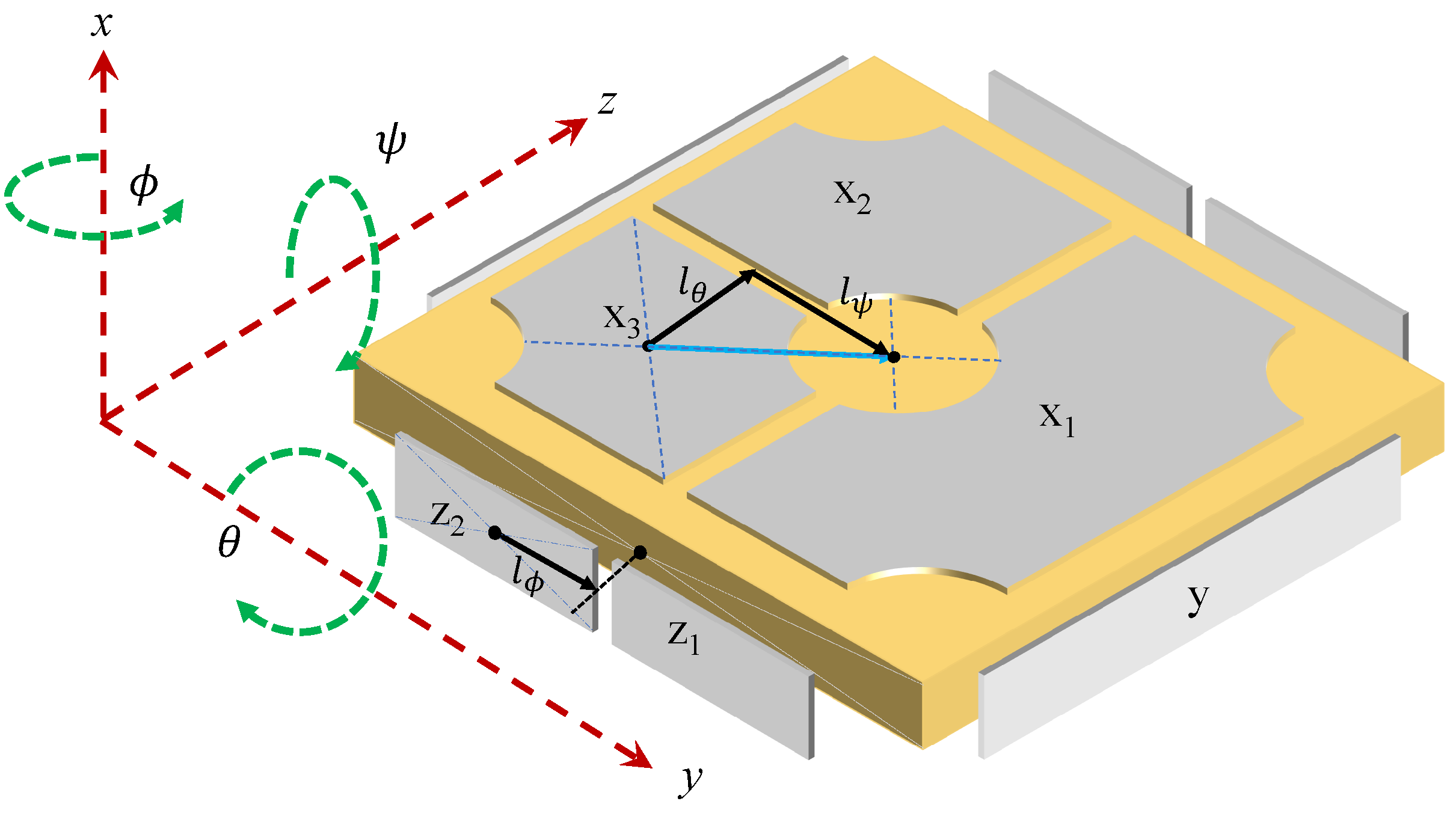
is the total area of electrode surface of the ith axis, D i the nominal distance between the TM surface and the electrode, and l i denotes the force arm of the electrodes pair that control the i t h rotation degree of freedom (see again Figure 3). ϵ 0 stands for the vacuum permittivity, and V P stands for the preload-biased voltage. The values of these parameters for Taiji-1 are shown in Table 1, and the transformation relations between the actuation voltages and compensation accelerations are shown in Table 3.
According to the designs of the Taiji-1’s IS system, we have the following useful relations in calibrating the linear scale factors and the COM offset,
β x = M l ϕ 2 J ϕ k z ,
β y = M l θ 2 J θ k x ,
β z = M l ψ 2 J ψ k x .
These relations remained unchanged during the mission lifetime because they involve only the geometrical and mechanical properties of the TM and the electrode cage. The high machining accuracy ( δ l / l 10 4 ) of the TM and cage structures ensures that the relations between the scale factors are sufficiently accurate. In this case, where l θ = l ψ and J θ = J ψ , we have β y = β z . Another important property is that during the normal science operation of the IS in its ACC mode the TM is controlled to tightly follow the motions of the electrode cage or the spacecraft. For Taiji-1, the position fluctuations of the TM relative to each electrode surface are ≤ 10 2 pm / Hz 1 / 2 in the sensitive band. This means that the rotations of the TM and the spacecraft could be treated as precisely synchronized, that one has
ω T M = ω S C , ω ˙ T M = ω ˙ S C .
Here, ω T M , ω ˙ T M , ω S C , and ω ˙ S C denote the angular velocities and angular accelerations of the TM and the spacecraft, respectively.
Therefore, despite the offset between the installation orientations of the IS system and the star trackers, the measured angular velocities and accelerations of the spacecraft and the TM are interchangeable.
The rotations or attitude variations ω S C and ω ˙ S C of the spacecraft could be independently measured by on-board star trackers. This motivates us to make use of such attitude measurements to calibrate the scale factors, which is different from the former methods based on precision orbit determination (POD) data [21,
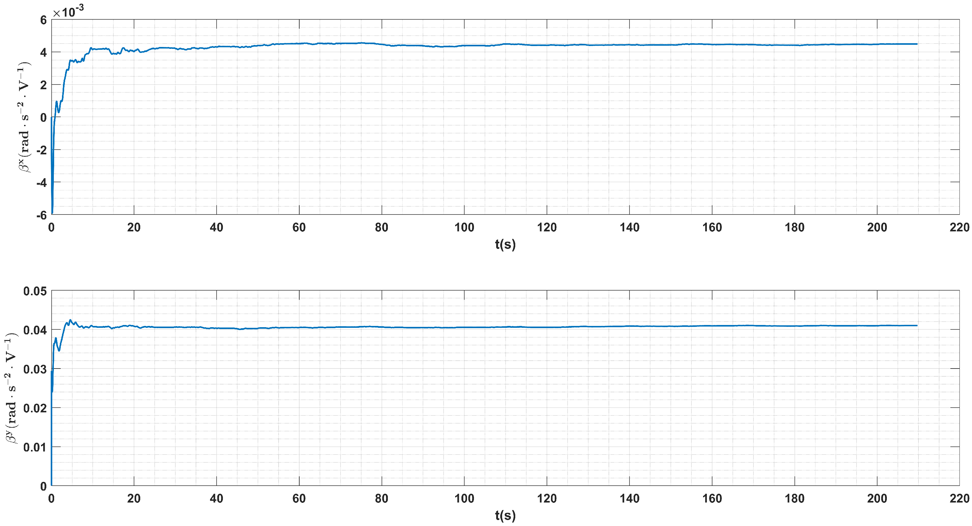
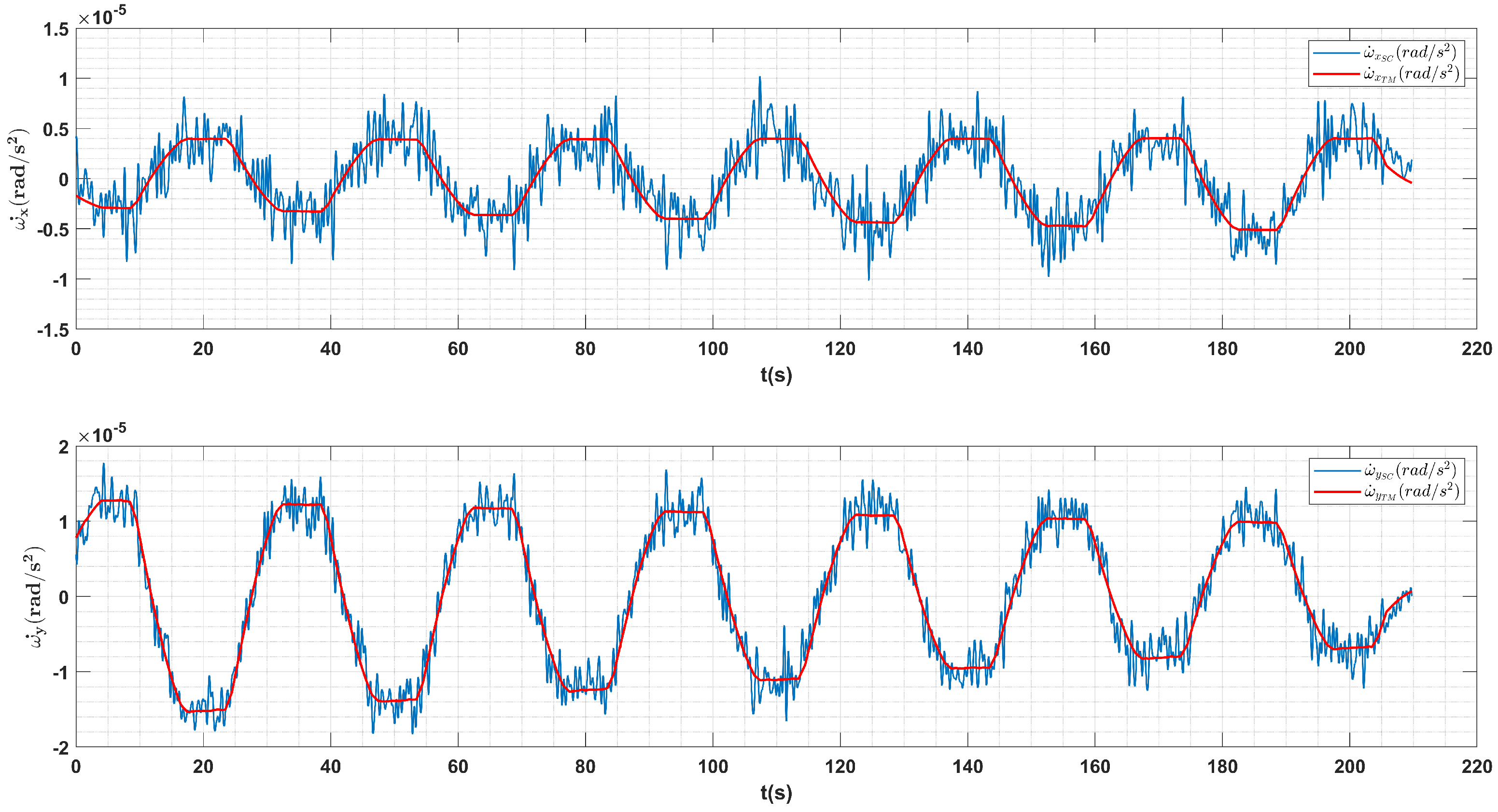
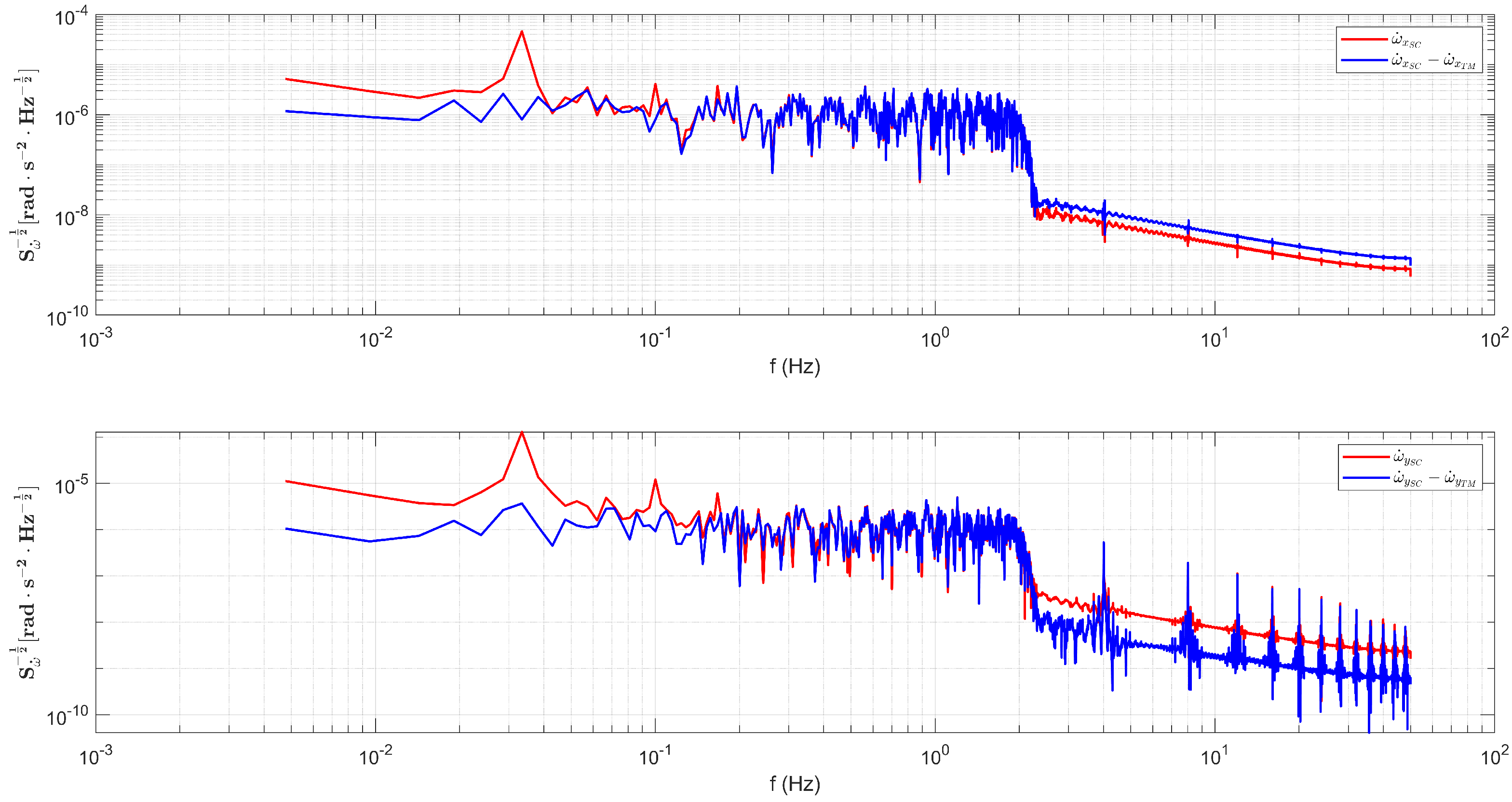
32]. One could swing the spacecraft periodically along a certain axis with a rather large angular accelerations and with relatively higher frequency compared to the signal band of air drags and solar radiations, which could be clearly identified and precisely measured by the IS system. With the inputs of the angular accelerations derived by the star track measurements and the actuation voltages readout by the front end electric unit of the IS system, one can fit the angular scale factors β i based on the equations in Table 3 with the least squares estimation or the Kalman filter algorithms. According to the relations between angular and linear scale factors in Equations (8)–(10), the linear scale factors can be further determined. For Taiji-1’s IS, controls along the y-axis are independent of other degrees of freedom, and their actuation voltage does not involve any rotation controls of the TM.
Therefore, the linear scale factor k y for Taiji-1’s IS system cannot be calibrated with this method and is left blank in this work. Please see 
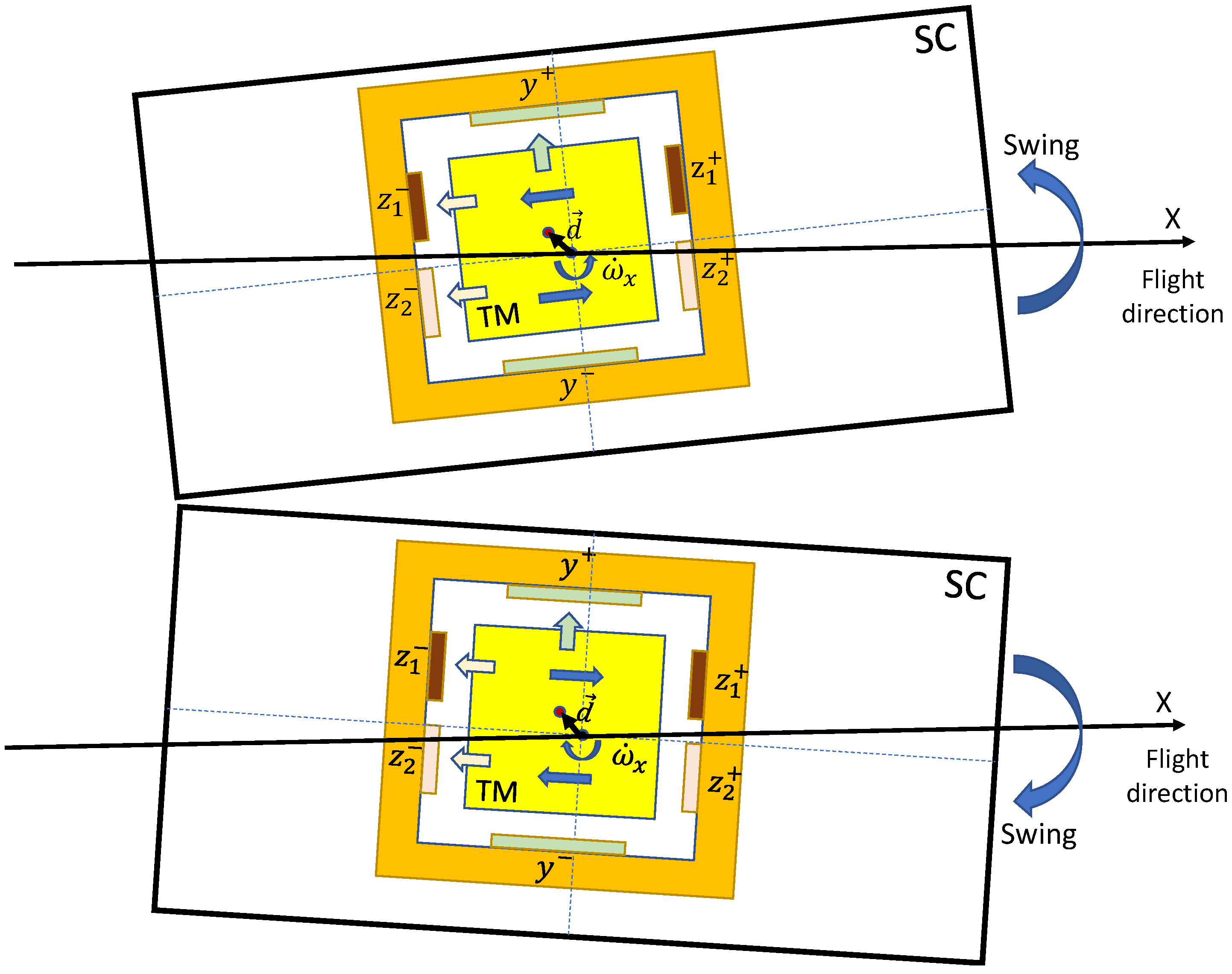
Figure 4 for an illustration of this calibration method.
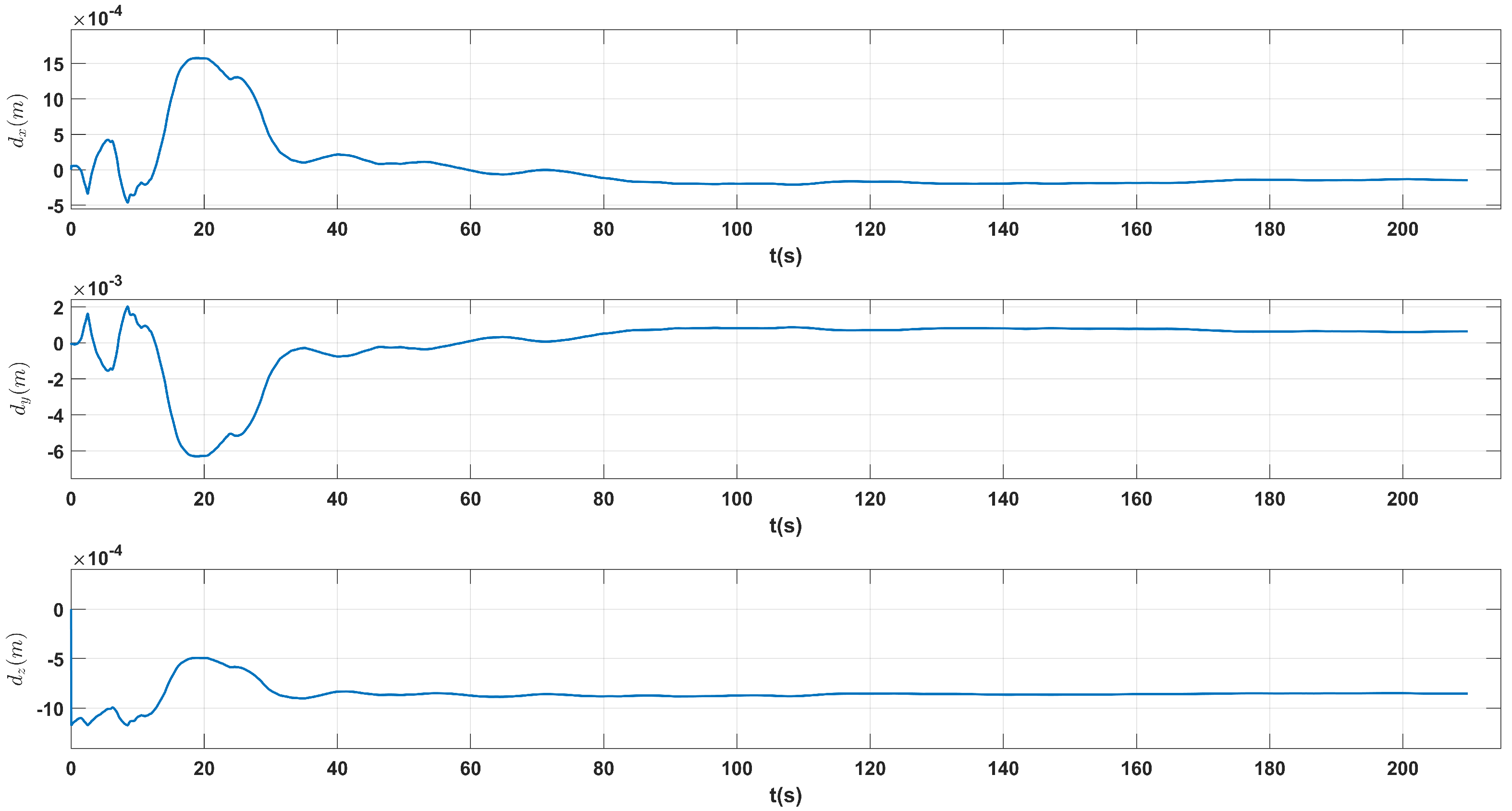
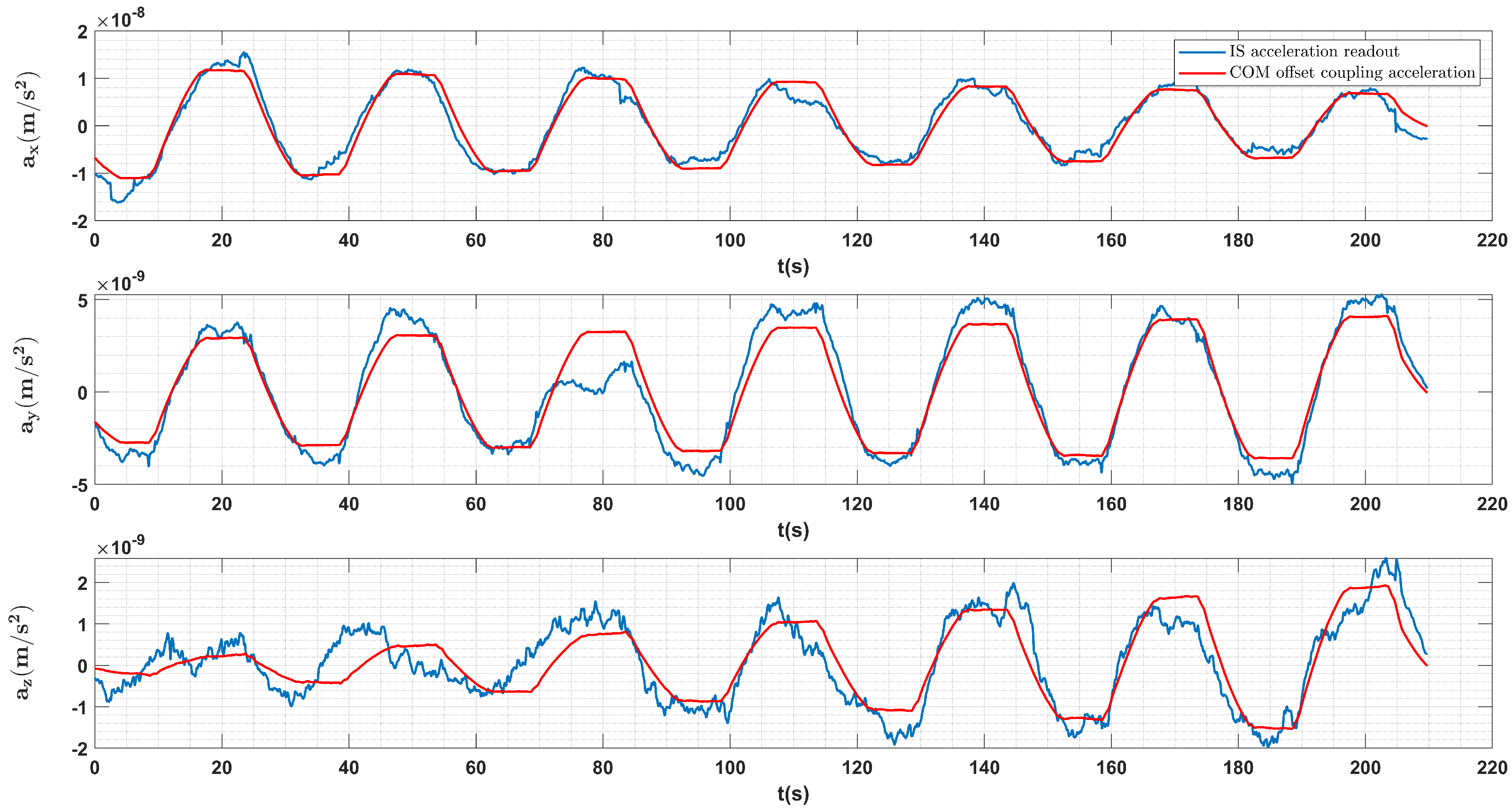
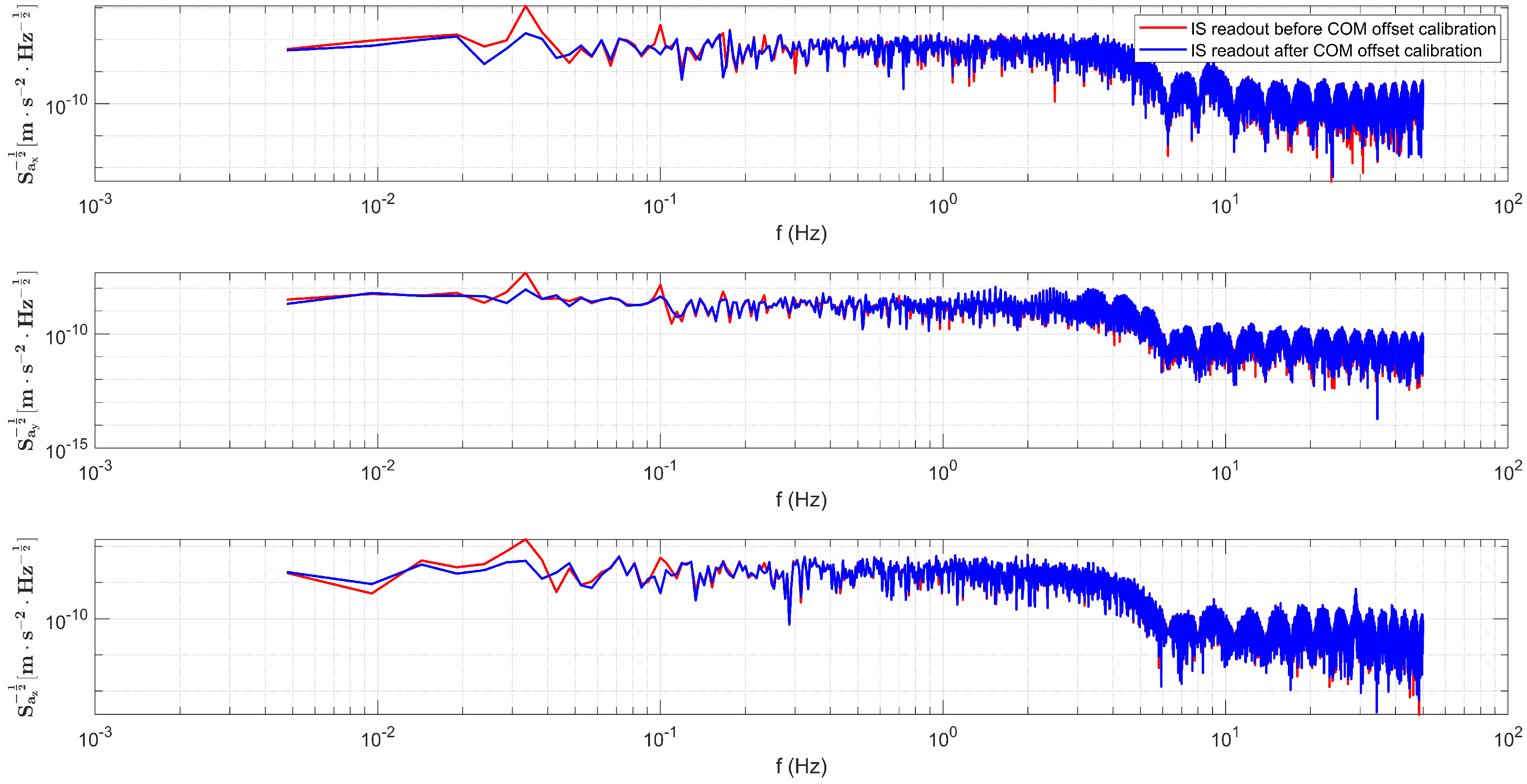
For the COM offset calibrations, one notices that according to Equations (2) and (3), the periodic swing of the spacecraft will also couple to the COM offset and produce periodic linear accelerations along the axes that are perpendicular to the rotation axis due to inertial effects, see again Figure 4. According to Table 3, one can then use the common mode readouts of the actuation voltages of each axis instead of the differential mode used in the scale factor calibrations, together with the spacecraft attitude data by the star trackers or the IS readouts itself to fit and calibrate the COM offset vector. This method was carefully studied and employed by the GRACE and GRACE-FO team [2,20,33,34]. However, one notices that possible interference may come from the gravity gradient signals because the spacecraft attitude variations would also produce periodic projections of the local gravity tidal force with the same frequency. This, on the contrary, forces us to choose satellite maneuvers with small magnitude of attitude variations. In fact, for Taiji-1 and GRACE-type missions, the magnitudes of gravity gradients ∼ 10 6 / s 2 . Therefore, according to Equation (2), for COM offset ≲ 10 3 m, attitude variations δ ω 10 3 rad will give rise to interference signals ≲ 10 12 m / s 2 , which could be safely ignored. However, to obtain larger calibration signals with small magnitude of attitude variations, one is then forced to swing the spacecraft with high frequencies that increases the magnitude of the last term ω i j ˙ d j in Equation (2). If the above considerations are satisfied, the remaining interference from the gravity gradients together with no-gravitational disturbances can be treated as a linear term due to the orbit evolutions and be filtered and removed in data processing.
For clarity, based on Equation (3) one can rewrite the observation equations for the COM calibration as
a c ( t ) = A ( t ) d + a I t + b I ,
where
A = ω y 2 ω z 2 ω x ω y ω ˙ z ω x ω z + ω ˙ y ω x ω y + ω ˙ z ω x 2 ω z 2 ω y ω z ω ˙ x ω x ω z + ω ˙ y ω y ω z + ω ˙ x ω z 2 ω x 2 .
Here, a I t + b I are the linear terms from the non-gravitational accelerations acting on the spacecraft and the gravity tidal accelerations coupled to the TM. Given the swing maneuvers discussed above, the COM offset vector d could then be fitted.
To summarize, we suggest calibration of the IS scale factors and COM offset with one round swing maneuver of the Taiji-1 satellite. To enhance the signal-to-noise ratio (SNR) and reduce the possible interferences, the swing maneuver should be of a high frequency compared with the signal band of non-gravitational forces, and the swing amplitude should be small to reduce the interference signals from gravitational tidal forces. Furthermore, the time span of the maneuver should be short to ensure that the linearity of the tidal force model remains sufficiently accurate. Finally, the attitude maneuvers should not be driven by thrusters, because the misalignment of the thrusters could produce large interference signals in linear accelerations in addition to the disturbances caused by propulsion. With these considerations, the maneuvers conducted by Taiji-1 were swings of the satellite driven by the magnetic torquers along a certain axis with a period of about 25∼30 s and a total time span of < 300 s. To enlarge the angular acceleration, we operated the magnetic torquers at their full powers, and the wave-trains of the satellite angular velocity were triangular waves with magnitudes of about 1 × 10 4 rad / s . The swing maneuvers were conducted on 18 May 2022, and data processing and fitting are discussed in the next section.

3.2. Principle of IS Bias Calibration

From a physical point of view, the intrinsic bias b i in the actuation acceleration measurements in Equation (5) mainly comes from the asymmetry of the electrodes on the opposite sides of the same axis and the imperfection in FEE unit. The imbalance of mass distributions surrounding the IS system, couplings between the TM and residual magnetic field, etc., may also contribute to the intrinsic bias accelerations. Therefore, the intrinsic bias along each axis is stable, and its changes could be ignored in short time measurements. On the contrary, the projections of the DC or very-low-frequency non-gravitational forces along each axis change not only with the orbit positions but also with the attitude of the satellite.
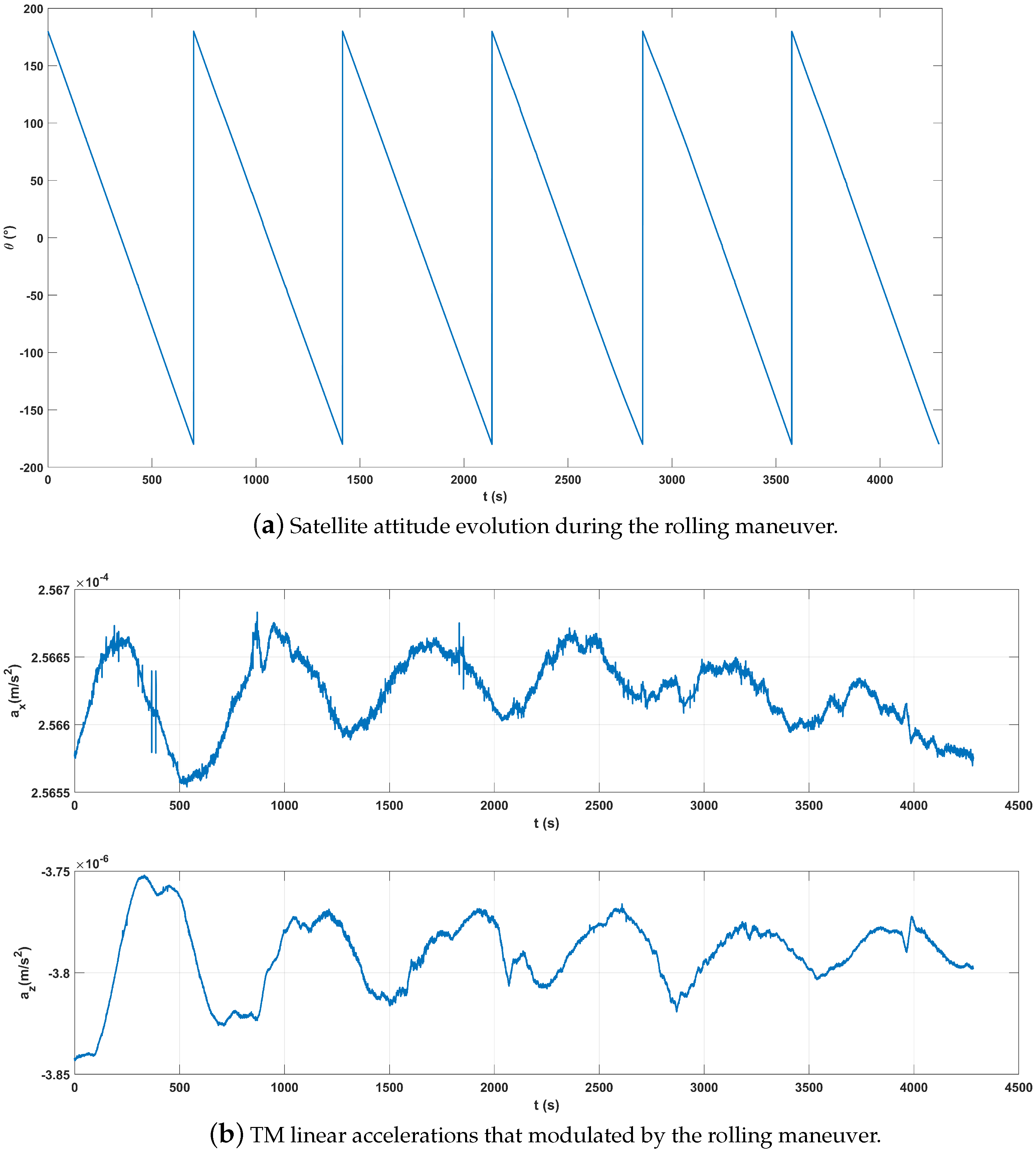
Generally, the long-term energy loss due to orbital decays based on the POD data and the work performed by the drag forces evaluated by the IS data need to be balanced, which gives us a method to determine the intrinsic biases; however, such a calibration method requires rather long-term and continuous observations and precise data from Earth geopotentials as inputs. For related missions, to avoid these technical difficulties and to make use of the IS data in time, we suggest here to roll the satellite to allow a quick calibration of the intrinsic biases with only the in-orbit measurements as inputs.
According to Equations (3) and (4), for the rolling maneuver, we rewrite the actuation acceleration measurements as
a c i ( t ) = b i + k 1 i α V α ( t ) = J = 1 3 a p a r a , S C J ( t ) cos ( Θ i J ( t ) + Θ 0 i J ) G i j ( t ) d j + a p a r a , T M i , k 1 i α V α ( t ) = b i + J = 1 3 a p a r a , S C J ( t ) cos ( Θ i J ( t ) + Θ 0 i J ) G i j ( t ) d j + a p a r a , T M i .
Here, a p a r a , S C J with ( J = X , Y , Z ) denotes the components of the non-gravitational accelerations exerted by the satellite in the orbit coordinates system. Θ i J is the angle between the ith axis of the IS system and the 
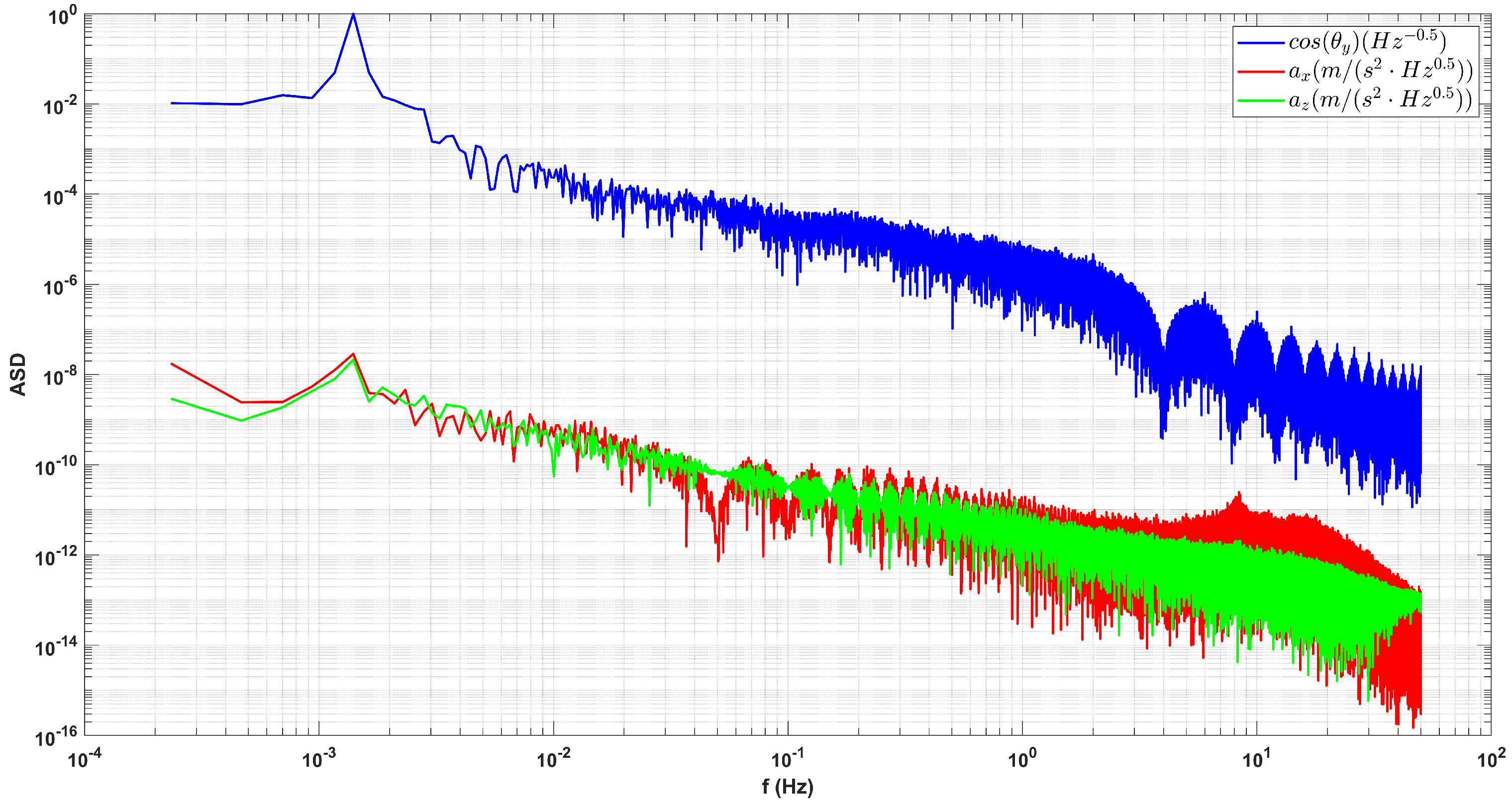
Jth axis of the orbit coordinates system. This rolling modulation will separate the DC and low-frequency non-gravitational forces from the intrinsic biases of the IS in the linear acceleration measurements and could be subtracted or averaged out from the data to suppress their effects on bias estimations.
For practical use, this method benefits when the maneuver time span for each estimation was short, that for short orbital arcs the non-gravitational forces could be treated as varies linearly with time,
a p a r a , S C J ( t ) = a J t + a 0 J .
The input data sets include the angles Θ i J , which can be derived by the POD data from GPS or Beidou system and the satellite attitude data from the star trackers, the actuation voltages that are readout by the FEE unit of the IS, the scale factors, and the calibrated COM offset.
The periodic terms a p a r a , S C J ( t ) cos ( Θ i J ( t ) + Θ 0 i J ) on the right-hand side of Equation (14) can be fitted and subtracted from the IS actuation accelerations. Generally, with the in-orbit center of mass adjustment for the satellite platform, the COM offset term G i j ( t ) d j could then be ignored in the data fits. If not, the G i j ( t ) d j term could also be modeled with the above input data and subtracted from the IS readouts. Then, the biases can be estimated based on the above observation Equation (14). For Taiji-1, to fulfill the requirement discussed above, the rolling period of the satellite was about 724 s, and to test the effectiveness of this method and also to accumulate data segments with better qualities, the entire time span of the rolling maneuver was 1.6 × 10 6 s.
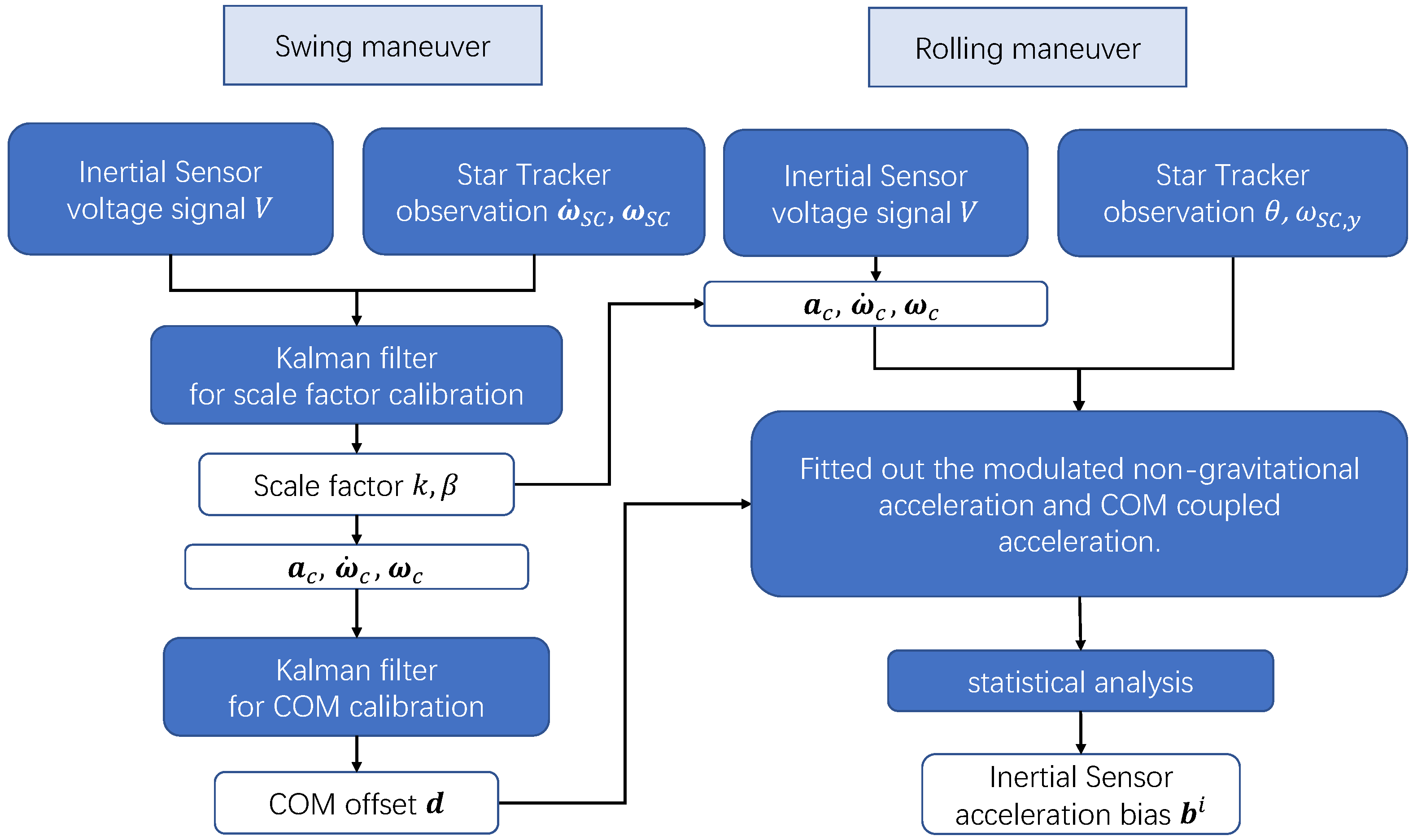
To conclude this section, the complete calibration process of the scale factors, COM offset and IS biases is summarized in Figure 5.

4. Calibration Results

In 2022, the final extended phase of Taiji-1, many experiments were planned and performed nonetheless. The swing maneuvers for the IS scale factors and COM offset calibrations were conducted for several trials with slightly different frequencies to obtain more accurate triangular wave trains of the SC/TM angular velocities or square wave trains of the angular accelerations. In this work, the scale factors and COM offset calibrations are based on the data of the swing maneuver conducted on 18 May 2022. After the encounter of the satellite with the Earth’s shadow, the calibration experiments were continued in August 2022. The rolling maneuver for IS bias calibration was conducted beginning in August 2022 and lasted for about 1.6 × 10 6 s to accumulate enough data. The detailed data processing procedures and fitting algorithms are expanded upon in the following subsections.

4.1. Swing Maneuver and Data Preprocessing

As discussed in Section 3.1, for scale factors and COM offset calibrations, the related data products are the IS actuation voltages readouts and the satellite attitude data from star trackers. The POD data from the Beidou or GPS system are also required to determine the position of the satellite and the local orbital coordinates system. Then, the satellite attitude variations in the local orbital coordinates system are derived first. According to the calibration principles, the Fourier components of the swing frequency and its harmonics in the data are used to fit the corresponding parameters. To reduce possible interferences from high-frequency noises (mainly comes from the FEE unit) and long-time drifts, the actuation voltages and attitude data are detrended, and then smoothed with low path filters. The low-path filter used here is the CRN filter (a classical digital filter characterized by an N-th order self-convolution of rectangular time-domain window function) with a cut-off frequency of 0.1 Hz. See Figure 6, Figure 7, Figure 8 and Figure 9 for illustrations of the attitude and IS voltage data.
From these figures, one sees that the projections of the swings along the z-axis (IS frame) is rather obscure. This is acceptable as it is mentioned in the previous section that for Taiji-1’s IS the scale factor k y can not be calibrated by this method, and for the COM offset calibrations, only swings along two different orthogonal axes are needed because of the redundancy. The outliers or spikes, for example the V x 1 data, are kept in the data, because no evident correspondence between such possible “data anomalies” with any instruments or payload events are found.

4.2. Results of Scale Factor Calibrations

As discussed in Section 3.1, our approach is based on the relations between the linear and angular scale factors showed in Equations (8)–(10). These equations depend only on the parameters of the TM, which can be measured precisely before launch and hardly change during the mission lifetime. Therefore, with the data from the IS and star trackers, one calibrates the angular scale factors first, and then with Equations (8)–(10), the estimations of the linear scale factors could be obtained.
After the preparations of the IS voltages and satellite attitude data sets, base on the method discussed in Section 3.1, the angular scale factors of Taiji-1’s IS ([ β x , β y , β z ] with β y = β z ) can be estimated by means of the following algorithms of Kalman filters
x n + 1 = Φ n x n + Γ n u n + Υ n w n ,
y ^ n = H n x n + ϵ n .
For the sequential least-square algorithm, we found that the estimations were hard to converge and oscillated around the mean values. The Kalman filter algorithm is adopted here because it is further adjusted in the Kalman gain matrix, which helps to improve the performance of the estimator. The above equations are the standard form of the discrete-time linear Kalman filter, Φ is the state transition matrix, Γ is the gain of the input u in the prediction/propagation equation, and Υ is the gain of the noise w of the dynamics of the estimator x. The number n represents the sample or the step number and the “ ^ ” labels the estimation values. Here, the estimator x, input y, and model matrix H are defined as
x = [ β x , β y ] T ,
y = [ ω ˙ x , ω ˙ y ] T ,
H = V z 1 V z 2 0 0 V x 2 V x 3 . .
Because β x and β y are constant parameters without dynamic feature, we have
Φ k = 1 , Γ k = Υ k = 0 .
In this case, to minimize the measurement noise ϵ , the Kalman filter equations can be rewritten as
x ^ n + 1 = x n + K n ( y ^ n H n x ^ n ) ,
K n = P n H n T [ ( H n P n H n T ) + R n ] 1 ,
P n + 1 = [ I K n H n ] P n ,
where the error covariance matrix P and variance matrix R of the measurement noise are defined as
P n = E { x ^ n x ^ n T } ,
R n = E { ϵ ^ n ϵ ^ n T } .
The initial values P 0 = E { x ^ 0 x ^ 0 T } and R 0 = E { ϵ ^ 0 ϵ ^ 0 T } are obtained from a prior calibration model using the sequential least-square method.
With this algorithm and the prepared data from the swing maneuver, the angular scale factors β x and β y convergent rather fast to their estimated values (see Figure 10 for illustrations). In this work, the accuracies of determining the parameters in Kalman filters are adopted as the standard deviations of the estimated values after they had converged.
The comparisons between the angular accelerations from the star trackers and the modeled actuation voltages with calibrated scale factors are shown in Figure 11, and their residuals are shown in Figure 12.
Finally, with the relations Equations (8) and (9), the complete scale factors calibrated with this method together with their estimation errors are listed in Table 4.

4.3. Results of COM Calibration

With the re-calibrated scale factors, the actuation voltage signals of the IS are transformed to the linear compensation acceleration a c i and angular compensation acceleration ω ˙ c i . Compared with the star tracker data, the attitude variation signals of the TM (or the satellite) measured by the IS have a better SNR. Therefore, based on the discussion in the previous section, where during the swing maneuver the IS was in its normal ACC mode and the TM tightly followed the rotations of the satellite platform, we will use the attitude variation data ω ˙ T M measured by the IS instead of ω ˙ S C derived by the star trackers data in the following COM offset calibrations.
The estimation algorithm based on Kalman filters is the same as that for the scale factors estimations in the previous subsection. The COM offset vector d is an unknown constant vector without dynamical features; therefore, the equations of parameter estimations can be re-written in the form of Equations (21)–(25). Here, for the case of COM offset calibration, the estimator x, input y and model H are
x = [ d x , d y , d z ] T , y = [ a x , a y , a z ] T , H = A ( ω i , ω ˙ i ) ,
where A ( ω , ω ˙ ) are defined in Equation (13).
The convergences of the COM offset components are shown in Figure 13. The comparisons between the measured linear acceleration (after pre-processing) and the modeled inertial accelerations with the re-calibrated values d i are shown in Figure 14. The re-calibrated COM offset vector is suggested to the Taiji-1 science team, and in practical use, the inertial accelerations are to be modeled given the attitude data and COM offset values and subtracted from the linear acceleration data (COM correction). The ASD curves of the TM’s linear accelerations before and after the COM corrections during the swing maneuver can be found in Figure 15, and with the estimated values d i , the peaks of the inertial accelerations are successfully identified and removed.
Finally, the calibrated COM offset values and their estimation errors are listed in Table 5. After nearly three years of operation, the magnitudes of Taiji-1 COM offset are still within the order of 10 2 μ m, while its long-term changes are also evident with respect to its nominal values.

4.4. Results of Bias Calibration

Based on the principle of bias calibration discussed in Section 3.2, the Taiji-1 satellite performed a long-duration uniform rolling maneuver along the y-axis (IS frame) in August 2022, which lasted for about 1.6 × 10 6 s (∼19 days). The rolling periods were short, ∼724 s, such that a data segment about 2000∼3000 s long would contain several rolling periods and the linear approximations of the non-gravitational forces in Equation (15) could be applied. A segment of the time series data of the satellite attitude evolution θ ( t ) along y-axis is shown in Figure 16a, and the linear accelerations modulated by the rollings in the x-axis and z-axis are shown in Figure 16b. Their ASD curves can be found in Figure 17.
One can see that in Figure 16b, the amplitudes evolutions of the oscillating signals in the TM linear acceleration measurements agree well with the linear model from Equation (15),
J = 1 3 a p a r a , S C J ( t ) cos ( Θ i J ( t ) + Θ 0 i J ) = J = 1 3 [ a J t cos ( Θ i J ( t ) + Θ 0 i J ) + a 0 J cos ( Θ i J ( t ) + Θ 0 i J ) ] .
Other long-term trends due to orbital evolution (see the linear acceleration in x-axis in Figure 16b as an example) can be fit with quadratic or cubic polynomial fitting methods.
The estimation procedure for the intrinsic biases of Taiji-1’s IS can be summarized as the following five steps: (1) preprocessing including data segmentation and quality check, (2) fitting trends in the TM linear accelerations due to orbital evolutions, (3) fitting the oscillating non-gravitational signals and the COM offset coupled signals, (4) estimations of the biases, and (5) statistical analysis of the estimations for each data segment. In preprocessing, the entire data set of the rolling maneuver is divided into short data segments with only a few rolling periods. The data quality of each segment was checked, and we choose only the data segments that have a more uniform rolling rate. About 300 data segments with different lengths were used in the bias calibrations, and the final estimations (see Table 6) were obtained from the statistical analysis of the calibration results for each segment.

4.5. IS Performance Evaluation

With all the necessary operating parameters having been calibrated in this work, the performance of Taiji-1’s IS system should be re-estimated with the updated parameters. In previous works [7,19], the performance or resolution level was obtained based on the y-axis measurements, because the projections of the non-gravitational forces, such as air drags, etc., in the orbital normal direction are small in comparison with those in the flight direction. However, as discussed in the previous sections, the scale factors k y cannot be calibrated with our new method; therefore, the performance of the other sensitive axis, that the z-axis along the flight direction, is re-estimated and discussed here. The original estimation of the noise along this axis can be found in Figure 16(a) from [19] and in Figure 2(d) from [7], which is above the 3 × 10 9 m / s 2 / Hz 1 / 2 level from 1 mHz to 1 Hz and reaches approximately ∼ 10 8 m / s 2 / Hz 1 / 2 in the mHz band. Because the z-axis is more noisy, accurate estimation of the best performance level of the IS system will not be trivial, which is beyond the scope of this paper and will be left for future works.
Here, a data set of V z 1 , V z 2 in 2022 with good quality is selected for the performance evaluation. With the updated scale factors and biases, and after the COM corrections, the ASD curves of the TM linear accelerations a c z , which can be viewed as an estimation of the noise floor a p a r a , T M z in the z-axis measurement, are found in Figure 18. It is found that, compared with the previous results, the new noise floor or resolution level is improved and now below the 3 × 10 9 m / s 2 / Hz 1 / 2 level in the sensitive band, and even below the 10 9 m / s 2 / Hz 1 / 2 level in the mHz band. This conclusion requires more analysis and further investigations and is beyond the scope of this work.

5. Conclusions

In this work, for gravity recovery missions, we suggest a systematic approach to calibrate the most important operation parameters for space-borne electrostatic IS system with two sets of satellite maneuvers. The operating parameters considered include the scale factors and COM offset vector that can be calibrated through one swing maneuver, and the intrinsic bias accelerations that can be calibrated through rolling maneuvers. The time spans required for these satellite maneuvers depend on the accuracies of the specific IS payloads and the requirements on the precision of the parameter calibrations. The working principle of the electrostatic IS and the estimation principles for its operating parameters are discussed, and the corresponding observation equations derived.
This systematic approach was applied to the re-calibrations of Taiji-1’s IS system to study the drift and variations of the operating parameters after its two years operation. The two satellite maneuvers were conducted in May 2022 and August 2022, respectively. For Taiji-1, the short-time swing maneuver of about 200 s is sufficient for scale factors and COM offset calibrations, and a data segment of a few thousand seconds long from the rolling maneuver is enough for a preliminary calibration of the biases. The real rolling maneuver lasted for about 19 days, and this is for the accumulations of data segments with better qualities and for the improvement of the accuracy of the bias estimations. The scale factors, COM offset, and the intrinsic bias accelerations of Taiji-1’s IS are precisely calibrated with the in-orbit data. The linear scale factor k y of the y-axis can not be calibrated by our new method, and its updated value is left blank in this work. The complete set of re-calibrated parameters are relayed to the Taiji-1 science team and are archived in the Taiji-1 data center of CAS in Beijing for future use in data processing.
One of the main objectives of Taiji-1 was to evaluate the performance of the IS payload and test the related technologies. Therefore, with the IS operating parameters being updated, a re-estimation of the performance of the IS and the comparison with the former results should be undertaken. As mentioned, because the new scale factor for the best sensitive y-axis is not available, we re-processed the data of the z-axis and found that, compared with former results, the performance or noise floor is improved with the updated parameters. However, a complete evaluation of the best performance of Taiji-1’s IS system is not trivial, and this is beyond the scope of this paper and needs more in-depth investigations and analysis in future works. On the other hand, in the extended phase in 2022, the Taiji-1 satellite operated in a high–low satellite-to-satellite tracking mode and could provide us monthly data of global gravity field. The re-calibration of the IS could improve the accuracies of the measurements of non-gravitational forces that disturb the orbit motions of the satellite, and the Taiji-1’s global gravity model could be further updated.
At last but not least, this systematic approach could offer high reference value for the ACC or IS calibrations of gravity recovery missions such as the Chinese GRACE-type mission and the future planned Next-Generation Gravity Missions. Furthermore, it could provide some insight into the in-orbit calibrations of the ultra-precision IS for future GW space antennas, because the principle and technology inheritance between these two generations of the electrostatic IS payloads.

Author Contributions

P.X. and H.Z. designed the calibration experiments; D.Y., L.-E.Q., K.Q., S.W., Z.W. and Z.L. discussed the principles and approved the feasibility of this calibration experiments for Taiji-1; Z.C. uploaded the instructions to Taiji-1 and conducted the experiments; H.Z. and Z.Y. analyzed the data and completed the calibrations; H.Z. and P.X. composed the paper; P.X., L.-E.Q., Z.L., J.L. and Y.W. provided general guidance and revised this paper. All authors have read and agreed to the published version of the manuscript.

Funding

This work is supported by the National Key Research and Development Program of China No. 2020YFC2200601, No. 2020YFC2200602, and No. 2021YFC2201901; the Strategic Priority Research Program of the Chinese Academy of Sciences Grant No. XDA15020700 and XDA15018000; and program No. ZC-1050-2021-05-011 from the Experiments for Space Exploration Program and the Qian Xuesen Laboratory, China Academy of Space Technology.

Data Availability Statement

The data presented in this study are available on request from the Taiji science team. The data are not publicly available.

Acknowledgments

The authors acknowledge for the data resources from “National Space Science Data Center, National Science & Technology Infrastructure of China”.

Conflicts of Interest

The authors declare no conflict of interest.

References

  1. Reigber, C.; Lühr, H.; Schwintzer, P. CHAMP mission status. Adv. Space Res. 2002, 30, 129–134. [Google Scholar] [CrossRef]
  2. Davis, E.; Dunn, C.; Stanton, R.; Thomas, J. The GRACE Mission: Meeting the Technical Challenges. 1999. Available online: https://ntrs.nasa.gov/citations/20000052706 (accessed on 27 July 2023).
  3. Tapley, B.D.; Bettadpur, S.; Ries, J.C.; Thompson, P.F.; Watkins, M.M. GRACE measurements of mass variability in the Earth system. Science 2004, 305, 503–505. [Google Scholar] [CrossRef] [PubMed] [Green Version]
  4. Flechtner, F.; Morton, P.; Watkins, M.; Webb, F. Status of the GRACE follow-on mission. In Proceedings of Gravity, Geoid and Height Systems: Proceedings of the IAG Symposium GGHS2012, Venice, Italy, 9–12 October 2012; Springer: Berlin/Heidelberg, Germany, 2014; pp. 117–121. [Google Scholar]
  5. Dahle, C.; Flechtner, F.; Gruber, C.; König, R.; Michalak, G.; Neumayer, K.H. The Gravity Recovery and Climate Experiment Follow-On (GRACE-FO) mission. Surv. Geophys. 2019, 40, 1481–1506. [Google Scholar]
  6. Drinkwater, M.R.; Floberghagen, R.; Haagmans, R.; Muzi, D.; Popescu, A.; Van den Ijssel, J. GOCE: ESA’s first Earth Explorer Core Mission. Acta Astronaut. 2003, 53, 217–232. [Google Scholar]
  7. Wu, Y.L.; Luo, Z.R.; Wang, J.Y.; Bai, M. China’s first step towards probing the expanding universe and the nature of gravity using a space borne gravitational wave antenna. Commun. Phys. 2021, 4, 34. [Google Scholar]
  8. Wu, L.M.; Xu, P.; Zhao, S.H.; Qiang, L.E.; Luo, Z.R.; Wu, Y.L. Global Gravity Field Model from Taiji-1 Observations. Microgravity Sci. Technol. 2022, 34, 77. [Google Scholar] [CrossRef]
  9. McNamara, P.; Vitale, S.; Danzmann, K. LISA Pathfinder: Mission summary and early results. Class. Quantum Gravity 2019, 36, 080301. [Google Scholar]
  10. Amaro-Seoane, P.; Audley, H.; Babak, S.; Binetruy, P.; Berti, E.; Bohé, A.; Caprini, C.; Colpi, M.; Cornish, N.; Danzmann, K.; et al. Laser Interferometer Space Antenna (LISA) for Gravitational Wave Astronomy: A joint mission between ESA and NASA. Class. Quantum Gravity 2017, 34, 044001. [Google Scholar]
  11. Hu, W.R.; Wu, Y.L. Taiji program in space for gravitational wave physics and nature of gravity. Natl. Sci. Rev. 2017, 4, 685–686. [Google Scholar] [CrossRef]
  12. Luo, J.; Chen, L.S.; Duan, H.Z.; Gong, Y.G.; Hu, S.; Ji, J.; Liu, Q.; Mei, J.; Milyukov, V.; Sazhin, M.; et al. TianQin: A space-borne gravitational wave detector. Class. Quantum Gravity 2016, 33, 035010. [Google Scholar] [CrossRef] [Green Version]
  13. Rehm, C.; König, R.; Jahr, T.; Maier, A.; Neumayer, H.; Schwintzer, P. CHAMP accelerometer data processing: Orbit determination and gravity field recovery. J. Geod. 2000, 74, 8–18. [Google Scholar]
  14. Ries, J.C.; Tapley, B.D.; Bettadpur, S. Design, implementation, and performance of the GRACE inertial instrument. Adv. Space Res. 2001, 28, 1835–1841. [Google Scholar]
  15. Floberghagen, R.; Fehringer, M.; Gruber, C.; Muzi, D.; Rothacher, M.; Jäggi, A.; Schrama, E.; Beer, S.; Kruizinga, G.; Pail, R.; et al. The gravity field and steady-state ocean circulation explorer mission: Mission overview and geodetic results. Surv. Geophys. 2013, 34, 511–550. [Google Scholar]
  16. Luo, Z.R.; Wang, Y.; Wu, Y.L.; Hu, W.R.; Jin, G. The Taiji program: A concise overview. Prog. Theor. Exp. Phys. 2021, 2021, 05A108. [Google Scholar] [CrossRef]
  17. Luo, Z.R.; Guo, Z.K.; Jin, G.; Wu, Y.L.; Hu, W.R. A brief analysis to Taiji: Science and technology. Results Phys. 2020, 16, 102918. [Google Scholar] [CrossRef]
  18. Ruan, W.H.; Guo, Z.K.; Cai, R.G.; Zhang, Y.Z. Taiji program: Gravitational-wave sources. Int. J. Mod. Phys. A 2020, 35, 2050075. [Google Scholar] [CrossRef]
  19. Wang, Z.; Lei, J.G.; On behalf of Taiji Scientific Collaboration. Development and on orbit test of Taiji-1 inertial reference. Int. J. Mod. Phys. A 2021, 36, 2140008. [Google Scholar] [CrossRef]
  20. Wang, F.R. Study on Center of Mass Calibration and K-Band Ranging System Calibration of the GRACE Mission; The University of Texas at Austin: Austin, TX, USA, 2003. [Google Scholar]
  21. Van Helleputte, T.; Doornbos, E.; Visser, P. CHAMP and GRACE accelerometer calibration by GPS-based orbit determination. Adv. Space Res. 2009, 43, 1890–1896. [Google Scholar] [CrossRef]
  22. Armano, M.; Audley, H.; Auger, G.; Baird, J.T.; Bassan, M.; Binetruy, P.; Born, M.; Bortoluzzi, D.; Brandt, N.; Caleno, M.; et al. Sub-femto-g free fall for space-based gravitational wave observatories: LISA pathfinder results. Phys. Rev. Lett. 2016, 116, 231101. [Google Scholar] [CrossRef] [Green Version]
  23. Baghi, Q.; Korsakova, N.; Slutsky, J.; Castelli, E.; Karnesis, N.; Bayle, J.B. Detection and characterization of instrumental transients in LISA Pathfinder and their projection to LISA. Phys. Rev. D 2022, 105, 042002. [Google Scholar]
  24. Huang, Z.Y.; Li, S.S.; Cai, L.; Fan, D.; Huang, L.Y. Estimation of the Center of Mass of GRACE-Type Gravity Satellites. Remote Sens. 2022, 14, 4030. [Google Scholar] [CrossRef]
  25. Armano, M.; Audley, H.; Baird, J.; Binetruy, P.; Born, M.; Bortoluzzi, D.; Castelli, E.; Cavalleri, A.; Cesarini, A.; Cruise, A.; et al. Calibrating the system dynamics of LISA Pathfinder. Phys. Rev. D 2018, 97, 122002. [Google Scholar] [CrossRef] [Green Version]
  26. Armano, M.; Audley, H.; Auger, G.; Binetruy, P.; Born, M.; Bortoluzzi, D.; Brandt, N.; Bursi, A.; Caleno, M.; Cavalleri, A.; et al. Bayesian statistics for the calibration of the LISA Pathfinder experiment. J. Phys. Conf. Ser. 2015, 610, 012027. [Google Scholar] [CrossRef]
  27. Bezděk, A. Calibration of accelerometers aboard GRACE satellites by comparison with POD-based nongravitational accelerations. J. Geodyn. 2010, 50, 410–423. [Google Scholar] [CrossRef] [Green Version]
  28. Klinger, B.; Mayer-Gürr, T. The role of accelerometer data calibration within GRACE gravity field recovery: Results from ITSG-Grace2016. Adv. Space Res. 2016, 58, 1597–1609. [Google Scholar] [CrossRef] [Green Version]
  29. Behzadpour, S.; Mayer-Gürr, T.; Krauss, S. GRACE Follow-On Accelerometer Data Recovery. J. Geophys. Res. Solid Earth 2021, 126, e2020JB021297. [Google Scholar] [CrossRef]
  30. Cai, Z.M.; Deng, J.F.; On behalf of Taiji Scientific Collaboration. Satellite architecture and preliminary in-orbit experiment of Taiji-1. Int. J. Mod. Phys. A 2021, 36, 2140020. [Google Scholar] [CrossRef]
  31. Jin, H.B.; Xu, P.; On behalf of Taiji Scientific Collaboration. The pipeline of data processing for TAIJI-1 space mission in the TAIJI program for the detection of gravitational wave. Int. J. Mod. Phys. A 2021, 36, 2140025. [Google Scholar] [CrossRef]
  32. Wang, H.B.; Xiong, Y.Q.; Zhao, C.Y. New Calibration Method of Accelerometers in GRACE Satellites Based on Precise Solar Radiation Model. Chin. Astron. Astrophys. 2017, 41, 558–576. [Google Scholar]
  33. Christophe, B.; Boulanger, D.; Foulon, B.; Huynh, P.A.; Lebat, V.; Liorzou, F.; Perrot, E. A new generation of ultra-sensitive electrostatic accelerometers for GRACE follow-on and towards the next generation gravity missions. Acta Astronaut. 2015, 117, 1–7. [Google Scholar] [CrossRef]
  34. Flury, J.; Bettadpur, S.; Tapley, B.D. Precise accelerometry onboard the GRACE gravity field satellite mission. Adv. Space Res. 2008, 42, 1414–1423. [Google Scholar] [CrossRef]
Figure 1. Block diagram for the architecture of Taiji-1.
Remotesensing 15 03817 g001
Figure 2. The layout of the payloads of Taiji-1.
Remotesensing 15 03817 g002
Figure 3. Layout of the core mechanical assembly of the IS.
Remotesensing 15 03817 g003
Figure 4. Satellite swing maneuver for the calibrations of the scale factors and COM offset.
Remotesensing 15 03817 g004
Figure 5. The flow chart of the scale factors, COM offset, and acceleration bias calibrations.
Remotesensing 15 03817 g005
Figure 6. The angular velocity of the satellite measured by star tracker. The blue lines denote the data before detrending and the red lines denote the data after detrending.
Remotesensing 15 03817 g006
Figure 7. (a) Satellite angular velocities measured by star tracker, where red lines denote the raw readouts and blue lines denote the data filtered by CRN filter. (b) Satellite angular acceleration measured by star tracker. (c) The filtered satellite angular acceleration filtered by CRN filter.
Remotesensing 15 03817 g007
Figure 8. IS voltage readouts along x-axis during the swing maneuver.
Remotesensing 15 03817 g008
Figure 9. IS voltage readouts along z-axis during the swing maneuver.
Remotesensing 15 03817 g009
Figure 10. Convergences of the angular scale factors β x (top) and β y (bottom) in the estimations.
Remotesensing 15 03817 g010
Figure 11. The comparisons between the angular accelerations from the star trackers (blue lines) and the modeled actuation voltages with calibrated scale factors (red lines) during the swing maneuver.
Remotesensing 15 03817 g011
Figure 12. The blue lines are the ASD curves of the difference between the angular accelerations from the star trackers and the modeled actuation voltages with calibrated scale factors during the swing maneuver. The red lines are the ASD of the angular accelerations from the star trackers.
Remotesensing 15 03817 g012
Figure 13. Convergence of the COM offset d i in the estimations.
Remotesensing 15 03817 g013
Figure 14. Comparison between the filtered TM linear acceleration measurements (blue lines) and the modeled inertial accelerations with calibrated COM offset (red lines) during the swing maneuver.
Remotesensing 15 03817 g014
Figure 15. Comparisons of the ASD curves of the TM linear accelerations before (red lines) and after (blue lines) the COM corrections.
Remotesensing 15 03817 g015
Figure 16. (a) Attitude evolution of the satellite along y-axis during the rolling maneuver. (b) The TM linear accelerations along the x- and z-axes during the rolling maneuver.
Remotesensing 15 03817 g016
Figure 17. ASD curves of the attitude variation along y-axis and the TM linear acceleration measurements in the x- and z-axes during the rolling maneuver.
Remotesensing 15 03817 g017
Figure 18. The noise floor of the actuation acceleration in z-axis after the systematic calibrations of the IS.
Remotesensing 15 03817 g018
Table 1. Parameters related to the structures of the mechanical assembly.
Parameterx-Axis ( ϕ )y-Axis ( θ )z-Axis ( ψ )Units
l 8.00 × 10 3 10.45 × 10 3 10.45 × 10 3 m
J 1.9440 × 10 5 1.0328 × 10 5 1.0328 × 10 5 kg· m2
D 6.20 × 10 5 7.70 × 10 5 7.50 × 10 5 m
S 2.395 × 10 4 2.054 × 10 4 2.056 × 10 4 m2
Table 2. Key design requirements of Taiji-1 IS system.
ParameterNominal Value
Dynamic range 3 × 10 5 m/s2
Bandwidth10 mHz∼1 Hz
Position noise≤1 nm/Hz1/2
Actuation noise 2 × 10 5 V / Hz 1 / 2
Readout noise 2 × 10 5 V / Hz 1 / 2
Acceleration noise 3 × 10 9 m / s 2 / Hz 1 / 2
Table 3. The actuation accelerations, angular accelerations, and the corresponding scale factors.
Compensation Acceleration ReadoutsScale Factors and Actuation Voltages
a c x k x ( 2 V x 1 + V x 2 + V x 3 )
a c y k y V y
a c z k z ( V z 1 + V z 2 )
ω ˙ c x β x ( V z 1 V z 2 )
ω ˙ c y β y ( V x 2 V x 3 )
ω ˙ c z β z ( 2 V x 1 V x 2 V x 3 )
Table 4. Scale factor in-orbit calibration results compared with their nominal values and ground-based calibration values.
Scale FactorNominal ValuesCalibrated ValuesCalibrated Values
On-GroundIn-Orbit
k x ( m / ( s 2 · V ) ) 5.41 × 10 4 null 5.43 × 10 4 ± 3.73 × 10 6
k y ( m / ( s 2 · V ) ) 3.00 × 10 4 2.7 × 10 4 null
k z ( m / ( s 2 · V ) ) 1.58 × 10 4 1.45 × 10 4 1.14 × 10 4 ± 2.67 × 10 7
β x ( rad / ( s 2 · V ) ) 5.93 × 10 3 6.21 × 10 3 4.42 × 10 3 ± 2.81 × 10 5
β y ( rad / ( s 2 · V ) ) 3.82 × 10 2 null 4.08 × 10 2 ± 9.57 × 10 5
β z ( rad / ( s 2 · V ) ) 3.82 × 10 2 null 4.08 × 10 2 ± 9.57 × 10 5
Table 5. COM offset calibration results for Taiji-1’ IS system.
COM OffsetCalibrated Value (µm)Error (µm)
d x 140.02 ± 5.02
d y 627.75 ± 16.25
d z 896.46 ± 1.16
Table 6. Intrinsic bias in-orbit calibration results for Taiji-1’s IS.
Intrinsic Acceleration BiasCalibrated Value (m/s2)Error (m/s2)
a x 2.5840 × 10 4 ± 1.0173 × 10 8
a y 1.9488 × 10 5 ± 2.6347 × 10 8
a z 2.9887 × 10 6 ± 2.9443 × 10 9
Disclaimer/Publisher’s Note: The statements, opinions and data contained in all publications are solely those of the individual author(s) and contributor(s) and not of MDPI and/or the editor(s). MDPI and/or the editor(s) disclaim responsibility for any injury to people or property resulting from any ideas, methods, instructions or products referred to in the content.

