Article

Canopy-Height and Stand-Age Estimation in Northeast China at Sub-Compartment Level Using Multi-Resource Remote Sensing Data

1
School of Forestry, Northeast Forestry University, Harbin 150040, China
2
Key Laboratory of Sustainable Forest Ecosystem Management, Ministry of Education, Northeast Forestry University, Harbin 150040, China
3
Heilongjiang Academy of Forestry, Harbin 150040, China
*
Author to whom correspondence should be addressed.
Remote Sens. 2023, 15(15), 3738; https://doi.org/10.3390/rs15153738
Submission received: 2 June 2023 / Revised: 20 July 2023 / Accepted: 21 July 2023 / Published: 27 July 2023

Abstract

:
Stand age is a significant factor when investigating forest resource management. How to obtain age data at a sub-compartment level on a large regional scale conveniently and in real time has become an urgent scientific challenge in forestry research. In this study, we established two strategies for stand-age estimation at sub-compartment and pixel levels, specifically object-based and pixel-based approaches. First, the relationship between canopy height and stand age was established based on field measurement data, which was achieved at the Mao’er Mountain Experimental Forest Farm in 2020 and 2021. The stand age was estimated using the relationship between the canopy height, the stand age, and the canopy-height map, which was generated from multi-resource remote sensing data. The results showed that the validation accuracy of the object-based estimation results of the stand age and the canopy height was better than that of the pixel-based estimation results, with a root mean squared error (RMSE) increase of 40.17% and 33.47%, respectively. Then, the estimated stand age was divided into different age classes and compared with the forest inventory data (FID). As a comparison, the object-based estimation results had better consistency with the FID in the region of the broad-leaved forests and the coniferous forests. In addition, the pixel-based estimation results had better accuracy in the mixed forest regions. This study provided a reference for estimating stand age and met the requirements for stand-age data at the pixel and sub-compartment levels for studies involving different forestry applications.

Graphical Abstract

1. Introduction

The primary component of an ecosystem, forests contain the largest carbon pool of terrestrial ecosystems and significantly contribute to the world's carbon sinks [1]. A forest ecosystem, defined as a carbon source or carbon sink, is determined by its structure [2]. To account for and assess the carbon stocks of forest ecosystems, the spatial distribution mapping of the structure of the forest ecosystem was determined to be essential [3].
Stand age is defined as the mean of the tree age in one stand, and it is an important factor when investigating the factors involved in forest resource management [4]. The structure of the age has been considered the structure of the forest ecosystem, which may reflect the temporal and spatial changes in the carbon intensity in a forest ecosystem [5]. In general, younger forests are useful as carbon sinks while middle-aged forests are typically stronger carbon sinks, and mature forests are considered weaker or neutral carbon sinks [6]. In particular, some of the overly mature forests have even played a role as carbon sources [7]. The carbon exchange between a forest and its atmosphere changes with forest age [8]. To quantify the carbon pool, as well as the exchange capacity, of a forest ecosystem and to estimate the potential carbon strength of that ecosystem at both regional and global scales, it is crucial to understand the age structure and its geographical distribution [9].
The traditional method of obtaining a forest’s age has traditionally been labor and time intensive [10]. At the same time, traditional surveying methods could not obtain the spatial age distribution on a large scale, and carrying out a survey in remote areas with complex topography has been challenging [10]. Therefore, the issue of how to obtain age data on a large regional scale conveniently and in real time has become an urgent scientific challenge in forestry research. As compared to the limitations of traditional investigation methods, remote sensing technology has advantages for macro-scale investigations and has obtained ecological parameters of forests on both localized and large scales [11,12]. Remote sensing data, such as optical satellite images and radar data, have frequently been used to infer information related to forest stand age and structure [13].
Currently, two methods have been developed to estimate stand age using remote sensing data. One approach was to monitor any disturbances via remote sensing imagery. When a disturbance occurred, the forest structure and its function would be significantly changed [14,15]. For example, when clear-cutting or a forest fire transpired, the forest age was then defined as zero [16]. The age could then be recorded wherever forest management activities and forest fire events were frequently reported [17]. However, the recording of disturbances has not been well-documented in most regions. Therefore, long-time-series remote sensing data were used instead to detect changes and identify forest disturbances [18]. Once the long-term Landsat time-series stacks (LTSS) were opened for free access, disturbance detection methods were able to be rapidly developed based on these data [19]. A number of studies used a change-detection algorithm to extract various parameters based on different vegetation indices, and the results indicated that age information could be estimated by quantifying the parameters related to forest disturbance [20].
The second method of stand-age estimation was established by linking the stand age to the vertical parameters of a forest. It was challenging to reverse stand age since it was not directly sensitive to a remote sensing signal [21]. Therefore, an intermediate variable between the stand age and a remote sensing signal was required. The vertical structure was an important variable that had a strong correlation to age and, therefore, has frequently been used as an intermediate variable [22]. Canopy height was the most common and available structure, and this variable could be closely linked to stand age, particularly in even-aged forests [23]. Johannes et al. developed a regression model for the forest age estimation of Norwegian forests. Their findings showed that the site index and canopy height, which were obtained via airborne laser-scanning, were the most crucial factors in age modeling [24]. Zhang et al. obtained the forest-age mapping of China at a spatial resolution of 1 km using remote sensing and observational data. In addition, the connection between tree height and age was used to estimate the forest age using remote sensing. [14]. Yang et al. developed an approach for age estimation based on multi-resource remote sensing data, and the age was obtained using tree height, which had been estimated through optical satellite images and radar data [21]. Previous studies had indicated that the tree height could be directly acquired using remote sensing data [25,26], as it could be considered an intermediate parameter for age estimation. Although optical remote sensing technology had emerged earlier and had a rich spatiotemporal dataset, obtaining the vertical information of forests directly from the data was difficult [27]. The light detection and ranging (LiDAR) method, which is an active remote sensing technology acquiring global surface and target 3D information, has had an obvious advantage when extracting vertical information [28]. Combining the advantages of active and passive remote sensing data could overcome their individual limitations and provide an effective approach for forest age estimation.
In addition to the aforementioned challenges in forest age estimation, the research using remote sensing data has concentrated on matched measurements of individual pixels to develop a stand-age-estimation model and generate a stand-age map at the pixel level because the minimum unit of optical imagery is a pixel. However, in reality, the stand age of a patch, sub-compartment, or region would be more useful. Reyes-Palomeque et al. used the SPOT-5 multi-spectral images to carry out the segmentation process in order to generate a map of age classes, and the overall accuracy was 88.4–91.0% [29]. Moreover, they proposed that object-based classification allowed for better spectral separation.
The forest sub-compartment is the minimum object for information statistics and forest resource management, and it is also a basic unit of forest inventory. In addition, the natural characteristics within each sub-compartment, such as the condition of the stand, stand type, forest-age group, and species composition, were always similar but were significantly different from adjacent sub-compartments [30]. In addition, there were similar image features in the remote sensing imagery of a single sub-compartment, such as reflectance and texture features [31]. Establishing stand age at the sub-compartment level, which was considered the minimum unit to estimate, could reduce the remote sensing errors. Furthermore, forest managers would be more interested in the age estimation of sub-compartments and compartments, rather than a single stand.
To achieve this aim, we used an object-based approach based on multiple remote sensing datasets to estimate the stand age, and we compared the results between object-based and the pixel-based approaches. The objectives were as follows:
(1)
Establish the growth curves of broad-leaved, coniferous, and mixed forests, using the canopy height and stand age;
(2)
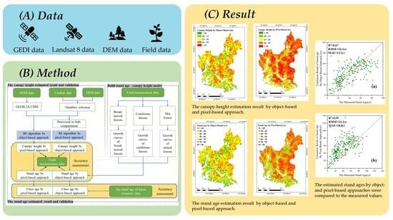
The generation of canopy-height maps from GEDI- and Landsat-extracted parameters;
(3)
Extract the remote sensing parameters according to object-based and pixel-based approaches;
(4)
Estimate stand age according to the canopy height and growth curves generated by the two approaches;
(5)
Compare the accuracy of the approaches for estimating stand age and canopy height.

2. Study Area and Remote Sensing Data

2.1. Study Area

The Mao’er Mountain Experimental Forest Farm in Shangzhi City, Heilongjiang Province, Northeast China, was the study site (127°29′–127°44′E, 45°14′–45°29′N) (Figure 1a). The research region was about 26.457 km2, and the forest land area was 22.694 km2. The landform of the research area was a low-mountain and hilly region. The average elevation was 300 m. The terrain gradually rose from south to north. The local climate zone belonged to the mid-temperate continental monsoon climate zone. The average forest cover was 83.29%, and the total forest volume was 3.5 million m3. The main tree species were birch (Betula spp.), Mongolica oak (Quercus spp.), larch (Larix spp.), Korean pine (Pinus koraiensis), Sylvestris pine (Pinus sylvestris), and poplar (Populus spp.) [32,33].

2.2. Remote Sensing Data and Pre-Processing

2.2.1. GEDI Data

The global ecosystem dynamics investigation (GEDI) LiDAR altimetry mission was launched in December 2018 [34]. The first multi-beam linear laser altimeter in the world was installed on the GEDI for measuring vertical structures globally with high quality, specifically for global-scale forest mapping [35]. The GEDI on the International Space Station was orbiting on board and measured canopy height, vertical structure, and elevation between 51.6° S and 51.6° N [34]. GEDI offered four different types of products, which included raw waveforms; footprint-level ground and canopy heights; grid-form heights; and biomass [34,36]. The raw GEDI waveform data were a Level-1 product [36]. Recently released on the Google Earth Engine (GEE), the GEDI Level-2A data offered canopy-relative height (RH) metrics, RH0-RH100 [37].
The GEDI Level-2A data contained 2 versions (Version 1 and Version 2). The recently released GEDI V2 significantly improved the precision and the validation of footprints [38], so the GEDI V2 available on GEE was used in this study (Figure 1b). The RH90 was extracted as RH data from GEDIL2A for each study location. All GEDI data from April to October was from 2019 to 2021 (the period of acquired leaf-on data, which was beneficial for the canopy height) was downloaded, and 30298 footprint points were obtained. To select the higher-quality canopy-height data, the footprint points were screened according to four rules:
① Footprint points acquired only using full-strength lasers [39,40];
② Beam sensitivity ≥0.9 [39];
③ Slope less than 30 degrees [20];
④ Footprint point must be located in forest land.
In the end, 7354 footprint points were retained according to these conditions. In addition, the footprint points were selected for the stand-age estimation. Data visualization was performed in Python (Version: 3.8).

2.2.2. Landsat 8 Data

The Landsat-8 Operational Land Imager (OLI) was an instrument of the Landsat series satellite, which was launched on February 11, 2013. The Landsat-8 OLI built on the Landsat series' history by adding 2 bands for cirrus clouds and a coastal/aerosol (CA) band for more accurate measurements [41]. Landsat-8 OLI images consisted of 11 spectral bands with a spatial resolution of 30 m. The images of the Landsat-8 data were obtained in June 2020 (Figure 1c). The pre-processed images and extracted variables were obtained from the GEE platform.

2.2.3. Field Data

Field data included forest inventory data and field measurement datasets. Forest inventory data (FID), which were collected in 2020, had 2271 broad-leaved forest sub-compartments, 569 coniferous forest sub-compartments, and 123 mixed forest sub-compartments (Figure 1d).
Field measurement data were obtained from 269 forest sample plots in 2020 and 2021, and these included 177 samples of broad-leaved forests, 65 samples of coniferous forests, and 27 samples of mixed forests. These samples were used to establish the growth model. The plot size was 0.06 ha. Field measurements included forest structural information, such as canopy height, stand age, forest type, etc. To reduce the variability in the survey data and the survey approach used on the sample sites, the stand-age data were corrected using the site–class index-oriented curve-fitting method by Li [42]. The statistical information of field measurements is shown in Table 1.

2.2.4. DEM Data

In order to extract terrain data, the SRTMGL1 digital elevation model (DEM) of the research area was acquired via the GEE platform. The data were extracted from version 3.0 at a 30 m spatial resolution, and the data were in HGT format. The slope data were extracted from the DEM data using ArcGIS (version 10.8.1, ESRI, Redlands, CA, USA).

3. Methodology

To estimate the stand age from the canopy height using remote sensing data, the following information was required: the definition of the growth model that compared the canopy height and stand age, the variable selection, and the retrieval algorithm for the canopy-height estimation. A technical flowchart of this research is shown in Figure 2.

3.1. Canopy-Height–Stand-Age Modeling

Vertical structure information has been highly correlated with stand age. Therefore, canopy height has often been considered a proxy for stand age. To infer the age, the growth curves of the three forest types (broad-leaved, coniferous, and mixed forests) were generated by the relationship between stand age (t) and canopy height (H). The models are shown in Table 2. In this study, we fitted both the base logistic-growth model [43] (H = f(t) and t = g(H) models) and a dummy model, where the dummy variable indicated the forest types (F). In the dummy model, the broad-leaved forests were set as X1 = 1, X2 = 0; the coniferous forests were set as X1 = 0, X2 = 1; and the mixed forests were set as X1 = 0, X2 = 0. The field-measured 269 sample plots were used to fit the base model and the dummy model of the Mao’er Mountain Experimental Forest Farm, using SPSS statistics software (SPSS 26.0, SPSS Inc., Chicago, IL, USA). Then, the determination coefficient (R2) and the root-mean-square error (RMSE) were calculated to assess the accuracy of the modeling.

3.2. Variable Selection for Canopy-Height Estimation from Remote Sensing Data

To achieve the canopy-height inversion, the first significant step was selecting the variables extracted from optical remote sensing data. To improve the independence of the variable dataset, the extracted parameters from Landsat-8 and the terrain factors extracted from DEM were selected as candidate characteristics [44]. A total of 67 variables were extracted from the satellite image data, which included 6 bands of Lansat-8 satellite data, 3 tassel-cap transformed components, 15 vegetation indices, 1 slope, and 42 texture features. These can be found in the supplementary material (Table S1).
Based on the methods of Yu et al., the correlation coefficient and variable importance were used to screen the candidate variables [45]. The correlation coefficient between the candidate variables and the canopy heights was used to screen the candidate variables. The value of the candidate variables could then be screened using the variable importance, which was used to evaluate the significance of the variables [46]. The importance values of the remaining variables, as determined by the previous step, were then calculated. The results varied according to the variable’s importance, and they also indicated the independent variables. In the end, eight remote sensing variables were found to be optimal for establishing the canopy-height estimation model. The details of these eight variables are shown in Table 3.

3.3. Random Forest Algorithm for Canopy-Height Modeling

The random forest (RF) algorithm was used to invert the canopy height in this study. RF is a non-parametric statistical estimation algorithm that did not depend on any assumptions about the relationship between the responses and the explanatory factors [47]. The advantages of RF included an insensitivity to noise, its ability to estimate the variable importance of the input sources, and its ability to handle a large amount of input [45]. As compared to other algorithms, the RF algorithm was insensitive to the values of its free parameters [48]. It has been widely used as a machine-learning technique for canopy-height estimation [38,49]. After repeated testing, the random state of the RF algorithm was set at 5, and the number of the regression trees was set at 200 [40,48]. The accuracy of the RF algorithm was calculated using a 10-fold cross-validation to eliminate overfitting. The RF algorithm was implemented using the Python scikit-learn package [50].

3.4. Object-Based/Pixel-Based Canopy-Height Estimation

In this study, the canopy height was estimated using both object-based and pixel-based approaches, as the latter approach had been the most commonly used method in the literature. In addition, the size of the pixel, or footprint, was the smallest unit of estimation (Figure 3). For the pixel-based estimation method, the pixels and the footprints of the forest lands were selected. First, the rasterized pixels and footprints were matched by spatial location information. Usually, there were two types of relationships between the pixels and the footprints, post-matching. For the first relationship, the footprint was converted into pixels, and then the DN values of the pixels could be extracted. The other relationship was formed when the footprint covered more than one pixel, which required the DN value to be recalculated. The DN value of the footprint was then determined by the weight of the area in each pixel. In addition, the DN value was equal to the sum of the proportional area of every pixel in the footprint, multiplied by the DN value of each pixel. Finally, the data pairs of the pixel features extracted from variable selection and the GEDI footprints were used to establish the canopy-height estimation method, using the RF algorithm.
For the object-based approach, the smallest unit was the sub-compartment (Figure 4). Therefore, the first step was to extract the image feature information at the sub-compartment scale. When the rasterized image and the GEDI footprint were matched with a sub-compartment, the multiple GEDI footprints would be classified as that sub-compartment. The mean information of these footprints was considered a representative value of the sub-compartment object. Similarly, the average of the pixel DN values in one sub-compartment was also considered a representative value of the sub-compartment. Then, the data pairs of the extracted variable selection and the canopy height could be established using the RF algorithm of the object-based method.

3.5. Validation

The following indices were applied for the accurate evaluation of the canopy-height model and stand age, which included the mean absolute error (MAE), the R2, and the RMSE. The equations were as follows [51]:
M A E = 1 n × i = 1 n y i y i ^
R 2 = 1 i = 1 n y i y i ^ 2 i = 1 n y i y ¯ 2
R M S E = 1 n × i = 1 n y i y i ^ 2
where y i is the measured value, y ¯ is the mean of the measurement, y i ^ is the estimated value, and n is the number of samples.

4. Results

4.1. Fitting the Growth Curve between Stand Age and Canopy Height

The functions of the base model (the logistic-growth model (H = f(t) and t = g(H) models)) and the dummy model were fitted by forest type. The results of the base models are shown in Table 4. The functions of the dummy model and the accuracy verification are shown in Table 5.
The higher R2 values and the lower RMSE values of the growth curve showed that the method used could produce more accurate estimates. Compared to the base model, we found that the regression model results of the dummy variable model M3 (T was added to the third parameter) had higher accuracy. Therefore, the dummy variable model M3 was used to establish the relationship between the canopy height and the stand age of the different forest types (Figure 5).

4.2. Object-Based and Pixel-Based Canopy-Height Modeling Result and Accuracy Assessment

In this paper, the GEDI data were linked to selected remote sensing variables using the RF algorithm to create a continuous canopy-height dataset in space. In addition, the canopy-height estimation results using object-based and pixel-based methods were calculated. Table 6 shows a comparison of the results between the two different approaches.
A total of 1636 samples were available for object-based modeling and validation. The R2 and RMSE of the object-based approach of the training set were 0.68 and 2.61 m, respectively, and the R2 and RMSE of the test set of the object-based approach were 0.57 and 2.87 m, respectively. A total of 6878 footprint points of the GEDI Lidar were used to build the RF model of the pixel-based approach. The R2 and RMSE of the training set of the object-based approach were 0.59 and 3.34 m, respectively, and the R2 and RMSE of the test set of the object-based approach were 0.51 and 3.57 m, respectively.
The estimated canopy heights from the two approaches were compared with the measured heights (Figure 6). According to the results of the object-based approach, the average canopy-height estimation was agreeable with the measured results at the sub-compartment scale. The R2, RMSE, and MAE were 0.72, 2.83 m, and 2.12 m, respectively (Figure 6a). According to the results of the pixel-based approach, the canopy-height estimation was obviously overestimated with the measured results. The R2, RMSE, and MAE were 0.63, 4.73 m, and 3.54 m, respectively (Figure 6b).
The canopy height was estimated using the RF algorithm and based on two approaches, and the canopy-height estimation results in the study area are shown in Figure 7. Then, the canopy-height estimation results were classified into five levels for a better comparison with the pixel-based results. In addition, the results estimated using the pixel-based methods were usually higher than those of the object-based methods (Figure 7a,b). To compare the differences between the two approaches, the pixel-based estimates were divided according to the boundaries of the sub-compartments (Figure 7c). In addition, the results were also not expected to be comparable to the results of the object-based estimation. This indicated that the object-based approach was valuable for applications on a sub-compartment scale.

4.3. Stand-Age-Estimation Results

The stand ages were mapped according to the canopy-height–stand-age model (Table 5-M3) and the object-based and pixel-based canopy-height estimation results. The calculated results are shown in Figure 8. In addition, the stand ages of different types and origins were classified into age classes according to the standards of the National Forestry and Grassland Administration of China, published in 2017 [52].
The estimated stand ages by object- and pixel-based approaches were compared to the measured values (Figure 9). Using the object-based approach, the R2, RMSE, and MAE were 0.67, 16.1 yr, and 12.1 yr, respectively (Figure 9a). For the pixel-based approach, the R2, RMSE, and MAE were 0.59, 24.2 yr, and 18.8 yr, respectively (Figure 9b). In addition, there was an obvious overestimation trend for the results of the pixel-based approach.
In order to evaluate the estimated age class of the two approaches, we compared the results with the FID. There were 2963 sub-compartments in the study area, including 513 young sub-compartments, 1006 middle-aged sub-compartments, 693 near-mature sub-compartments, 617 mature sub-compartments, and 134 over-mature sub-compartments. The proportions were 17.31%, 33.95%, 23.39%, 20.82%, and 4.52%, respectively. Overall, the estimated results of the stand-age class were consistent with the forest survey results. The object-based estimated stand-age classification included 442 young forest sub-compartments, 1016 middle-aged forest sub-compartments, 734 premature forest sub-compartments, 658 mature forest sub-compartments, and 113 over-mature forest sub-compartments. The proportions were 14.92%, 34.29%, 24.77%, 22.21%, and 3.81%, respectively. The estimated results of the pixel-based approach were significantly overestimated, compared to the results of the resource survey (3.24%, 17.58%, 32.74%, 30.41%, and 16.03%, respectively). Moreover, the estimation accuracy of the pixel-based approach for all the class ages was lower than the object-based estimation accuracy (Figure 10).

5. Discussion

5.1. Evaluation of the Stand-Age Estimation

Regression analysis has been a popular approach for fusing remote sensing data and biophysical factors in order to produce continuous estimations of features. Previous studies have indicated that many remote sensing parameters were significantly correlated with stand age [53,54]. However, the established relationship between stand age and remote sensing parameters varied with different research [55]. Additionally, stand age had been calculated using the inverted site index formulae that had previously been used to predict the expected height growth at various ages, as provided by foresters [24,56]. However, the site index curves were data-dependent, less robust, and associated with uncertainty. The canopy-height–stand-age curve, which had been defined by site-index equations, had also ignored the effects of disturbance information and species richness. To determine the relative relationship between canopy height and stand age using field measurement data, a nonlinear growth model was applied in this study. All the sample data were classified as either broad-leaved, coniferous, or mixed forests, and a nonlinear model was fitted. The fitted results showed that the models established by different forest types had higher accuracy than those using all samples. Next, the fitted models were used to estimate the canopy height, which was estimated using multi-resource remote sensing data, and the stand age was estimated using object-based and pixel-based approaches. This study demonstrated that the object-based stand-age-estimation model for the study area performed well during development and validation. The R2, RMSE, and MAE values were 0.67, 16.1 yr, and 12.1 yr, respectively. The accuracy of the pixel-based approach was lower than the object-based approach, and the R2, RMSE, and MAE were 0.59, 24.2 yr, and 18.8 yr, respectively. To further compare the results of the two approaches, the estimated stand ages of three different forest types were divided into young, middle-aged, premature, mature, and over-mature forests and then compared with the FID (Figure 11). The results indicated that the accuracy of the object-based approach was better than that of the pixel-based approach; the former had similar results with the stand age provided by the FID. The pixel-based approach had significant overestimations. There were two possible reasons for the overestimation. The first was that the noise from the bare-soil background land cover had influenced the spectral features of the young, open-canopy stands. The results demonstrated that accommodating the local spectral features (the object-based approach) mitigated the noise effect. The second reason was the overfitting of the RF algorithm, despite using a 10-fold cross-validation method to minimize this problem. Overfitting had caused higher canopy-height estimations that exceeded the boundary conditions of the canopy-height–stand-age curve, which had been set as the maximum value of the stand age. For these canopy heights, the stand ages were given values based on the upper-boundary canopy-height estimates. Because of this simplicity, the stand age of the higher-canopy-height forests might have been overestimated. In addition, the classification of the forest types could have been improved. In this study, the forest types were only divided into coniferous, broad-leaved, and mixed forests. If a more precise categorization of the tree species had been done, then the accuracy of the canopy-height estimation could have been improved significantly.

5.2. Comparison of Stand-Age Estimation at Pixel Scale and Sub-Compartment Scale

The object-based approach was commonly used to identify stand types [57]. Studies have used an object-based approach for classifications using satellite-imagery segmentation techniques and visual interpretations [29,58]. Lv et al. used a multiple-scale, object-based approach to estimate the above-ground carbon of stock bamboo forests, which obtained satisfactory results [59]. However, the basis of object segmentation remained focused on image segmentation. In this study, both object-based and pixel-based approaches were used to estimate stand age. The results indicated that the accuracy of the former was higher than that of the latter. There were two possible reasons for the high precision of the object-based estimation. The differences among the factors of one sub-compartment were a limitation when the minimum unit was one sub-compartment. In addition, the sub-compartments had similar natural characteristics and similar image features as well. Therefore, the differences among single pixels would have a cumulative effect on stand-age estimation. In addition, a nonlinear model of canopy-height–stand-age also increased the accuracy of the stand-age estimation. However, this effect could not be ignored in the pixel-based approach. Furthermore, the pixel-based approach estimated the individual pixels directly from the spectral information, but the accuracy had been reduced by the “same objects with different spectra” and “different objects with the same spectra” [59].
The results showed that the pixel-based approach performed better for the stand-age estimation of mixed forests. In this study, GEDI RH90 as the canopy height was input into the RF algorithm; GEDI RH90 has been regarded as the mean canopy height of footprints [40]. However, in the process of dividing the classes into age groups, the basis of the classification was the dominant species of the stands. Using the object-based approach, the canopy height of the dominant tree was smoothed, and the result of this approach showed underestimation. However, using a pixel-based approach, the estimations of the dominant species and the other species were mutually independent, so the estimated results had no influence. Therefore, the estimation of the object-based approach was more accurate. However, the results indicated lower precision when the pixels were unable to represent the objects adequately, especially at the boundaries of forested areas, where pixels included both forest canopy and land [29]. To confirm this conclusion, 27 samples of broad-leaved and coniferous forests were randomly extracted 10 times from the stand-age comparison data, as shown in Figure 9, and the results were compared with 27 samples of mixed forests by averaging the precision of the 10 extractions. The results are shown in Table 7. The object-based method had higher precision when estimating the stand age of broad-leaved and coniferous forests, and the pixel-based method performed better when estimating the stand age of mixed forests.

5.3. Uncertainty of Forest-Stand-Age Estimation

Though the stand-age-estimation approach indicated preferable potentialities, there were still uncertainties. First, the stand age was only developed by substituting spatial differences for time differences, which could have resulted in higher uncertainty regarding the stand-age estimates. This study did not consider the forest disturbances, and the estimated stand age only represented a normal forest. The temporal sequences of spectral values could be utilized to precisely identify when forest disturbances occurred in the satellite record; combining the two aforementioned methods could increase the estimation accuracy. Second, the canopy height was estimated according to the RF model, which was a black-box model with poor interpretability, leading to significant uncertainty. Third, a significant amount of field measurement data was needed to fit the growth curves of the different forest types; therefore, limiting the number of samples had an impact on the findings and the correctness of the fit. In addition, the GEDI footprints were sparse, which also affected the accuracy of the estimation results. If the ICESat-2 data could be integrated or advanced interpolation methods could be employed, the accuracy of the canopy height could be increased.

6. Conclusions

In this study, we estimated stand age using object-based and pixel-based approaches using canopy-height maps, which were generated via multi-resource remote sensing data. The following were the primary conclusions:
The base and dummy models were established to fit the relationship between the canopy height and the stand age. As a comparison, the results of the dummy variable model had a higher accuracy. With the help of the canopy-height–stand-age model, a map of the stand age was generated. The validation accuracy of the object-based estimation results was better than that of pixel-based estimation results, with RMSE improvements of 40.17% and 33.47%, respectively. The estimated stand age was then divided into age classes (young, middle-aged, premature, mature, and overmature forests) and compared with the FID. The object-based method had similar results regarding the stand age, as compared to the FID, but the results of the pixel-based approach were significantly overestimated. When comparing different forest types, the object-based method had higher accuracy in the stand-age estimations of broad-leaved forests (R2 = 0.53, RMSE = 16.6 yr, MAE = 13.5 yr), followed by coniferous forests (R2 = 0.81, RMSE = 10.2 yr, MAE = 8.6 yr). However, the pixel-based method performed better when estimating the stand age of mixed forests (R2 = 0.89, RMSE = 6.6 yr, MAE = 7.5 yr). This study provides a reference for estimating stand age and meets the requirements for stand-age data for studies on different forestry applications at pixel and sub-compartment levels.

Supplementary Materials

The following supporting information can be downloaded at: https://www.mdpi.com/article/10.3390/rs15153738/s1.

Author Contributions

Conceptualization, X.G. and X.Y.; methodology, Y.Y.; writing—review and editing: X.Y., Y.Y. and X.G.; reviewed: X.Y. and Y.Y.; software, Y.P., H.D. and T.Y. All authors have read and agreed to the published version of the manuscript.

Funding

This research was funded by the National Natural Science Foundation of China (grant numbers 31870621 and 31971580); the Fundamental Research Funds for the Central Universities of China (grant numbers 2572021BA08, 2572019BA10, and 2572019CP12); and the China Postdoctoral Science Foundation (grant number 2019M661239).

Conflicts of Interest

The authors declare no conflict of interest.

References

  1. Bonan, G.B. Forests and Climate Change: Forcings, Feedbacks, and the Climate Benefits of Forests. Science 2008, 320, 1444–1449. [Google Scholar] [CrossRef] [PubMed] [Green Version]
  2. Tang, X.; Zhao, X.; Bai, Y.; Tang, Z.; Wang, W.; Zhao, Y.; Wan, H.; Xie, Z.; Shi, X.; Wu, B. Carbon pools in China’s terrestrial ecosystems: New estimates based on an intensive field survey. Proc. Natl. Acad. Sci. USA 2018, 115, 4021–4026. [Google Scholar] [CrossRef] [Green Version]
  3. Jing, M.C. Carbon neutrality: Toward a sustainable future. Innovation 2021, 2, 1–2. [Google Scholar] [CrossRef]
  4. Brockerhoff, E.G.; Jactel, H.; Parrotta, J.A.; Ferraz, S.F.B. Role of eucalypt and other planted forests in biodiversity conservation and the provision of biodiversity-related ecosystem services. For. Ecol. Manag. 2013, 301, 43–50. [Google Scholar] [CrossRef]
  5. Pan, Y.; Chen, J.M.; Birdsey, R.; McCullough, K.; He, L.; Deng, F. Age structure and disturbance legacy of North American forests. Biogeosciences 2011, 8, 715–732. [Google Scholar] [CrossRef] [Green Version]
  6. Zhou, T.; Shi, P.; Jia, G.; Dai, Y.; Zhao, X.; Shangguan, W.; Du, L.; Wu, H.; Luo, Y. Age-dependent forest carbon sink: Estimation via inverse modeling. J. Geophys. Res. Biogeosci. 2015, 120, 2473–2492. [Google Scholar] [CrossRef] [Green Version]
  7. Wang, B.; Li, M.; Fan, W.; Yu, Y.; Chen, J.M. Relationship between Net Primary Productivity and Forest Stand Age under Different Site Conditions and Its Implications for Regional Carbon Cycle Study. Forests 2018, 9, 5. [Google Scholar] [CrossRef] [Green Version]
  8. Wang, X.; Wang, C.; Yu, G. Spatio-temporal patterns of forest carbon dioxide exchange based on global eddy covariance measurements. Sci. China Ser. D 2008, 51, 1129–1143. [Google Scholar] [CrossRef]
  9. Koedsin, W.; Huete, A. Mapping rubber tree stand age using Pléiades Satellite Imagery: A case study in Talang district, Phuket, Thailand. Eng. J. 2015, 19, 45–56. [Google Scholar] [CrossRef] [Green Version]
  10. Metsaranta, J.M. Dendrochronological procedures improve the precision and accuracy of tree and stand age estimates in the western Canadian boreal forest. For. Ecol. Manag. 2020, 457, 117657. [Google Scholar] [CrossRef]
  11. Bolton, D.K.; Tompalski, P.; Coops, N.C.; White, J.C.; Wulder, M.A.; Hermosilla, T.; Queinnec, M.; Luther, J.E.; van Lier, O.R.; Fournier, R.A.; et al. Optimizing Landsat time series length for regional mapping of lidar-derived forest structure. Remote Sens. Environ. 2020, 239, 111645. [Google Scholar] [CrossRef]
  12. Burns, P.; Clark, M.; Salas, L.; Hancock, S.; Leland, D.; Jantz, P.; Dubayah, R.; Goetz, S.J. Incorporating canopy structure from simulated GEDI lidar into bird species distribution models. Environ. Res. Lett. 2020, 15, 095002. [Google Scholar] [CrossRef]
  13. Lechner, A.M.; Foody, G.M.; Boyd, D.S. Applications in remote sensing to forest ecology and management. One Earth 2020, 2, 405–412. [Google Scholar] [CrossRef]
  14. Zhang, C.; Ju, W.; Chen, J.M.; Li, D.; Wang, X.; Fan, W.; Li, M.; Zan, M. Mapping forest stand age in China using remotely sensed forest height and observation data. J. Geophys. Res. Biogeosci. 2014, 119, 1163–1179. [Google Scholar] [CrossRef]
  15. Zhong, L.; Chen, Y.; Wang, X. Forest disturbance monitoring based on time series of Landsat data. Sci. Silvae Sin. 2020, 56, 80–88. [Google Scholar]
  16. Pflugmacher, D.; Cohen, W.B.; Kennedy, R.E.; Yang, Z. Using Landsat-derived disturbance and recovery history and lidar to map forest biomass dynamics. Remote Sens. Environ. 2014, 151, 124–137. [Google Scholar] [CrossRef]
  17. Vastaranta, M.; Niemi, M.; Wulder, M.A.; White, J.C.; Nurminen, K.; Litkey, P.; Honkavaara, E.; Holopainen, M.; Hyyppä, J. Forest stand age classification using time series of photogrammetrically derived digital surface models. Scand. J. For. Res. 2016, 31, 194–205. [Google Scholar] [CrossRef]
  18. Chen, G.; Thill, J.-C.; Anantsuksomsri, S.; Tontisirin, N.; Tao, R. Stand age estimation of rubber (Hevea brasiliensis) plantations using an integrated pixel-and object-based tree growth model and annual Landsat time series. ISPRS J. Photogramm. Remote Sens. 2018, 144, 94–104. [Google Scholar] [CrossRef]
  19. Huang, C.; Goward, S.N.; Masek, J.G.; Thomas, N.; Zhu, Z.; Vogelmann, J.E. An automated approach for reconstructing recent forest disturbance history using dense Landsat time series stacks. Remote Sens. Environ. 2010, 114, 183–198. [Google Scholar]
  20. Zhou, X.; Hao, Y.; Di, L.; Wang, X.; Chen, C.; Chen, Y.; Nagy, G.; Jancso, T. Improving GEDI Forest Canopy Height Products by Considering the Stand Age Factor Derived from Time-Series Remote Sensing Images: A Case Study in Fujian, China. Remote Sens. 2023, 15, 467. [Google Scholar] [CrossRef]
  21. Yang, X.; Liu, Y.; Wu, Z.; Yu, Y.; Li, F.; Fan, W. Forest age mapping based on multiple-resource remote sensing data. Environ. Monit. Assess. 2020, 192, 734. [Google Scholar] [CrossRef]
  22. Racine, E.B.; Coops, N.C.; St-Onge, B.; Bégin, J. Estimating forest stand age from LiDAR-derived predictors and nearest neighbor imputation. For. Sci. 2014, 60, 128–136. [Google Scholar] [CrossRef]
  23. Ung, C.-H.; Bernier, P.Y.; Raulier, F.; Fournier, R.A.; Lambert, M.-C.; Régnière, J. Biophysical site indices for shade tolerant and intolerant boreal species. For. Sci. 2001, 47, 83–95. [Google Scholar]
  24. Schumacher, J.; Hauglin, M.; Astrup, R.; Breidenbach, J. Mapping forest age using National Forest Inventory, airborne laser scanning, and Sentinel-2 data. For. Ecosyst. 2020, 7, 60. [Google Scholar] [CrossRef]
  25. Liu, X.; Su, Y.; Hu, T.; Yang, Q.; Liu, B.; Deng, Y.; Tang, H.; Tang, Z.; Fang, J.; Guo, Q. Neural network guided interpolation for mapping canopy height of China’s forests by integrating GEDI and ICESat-2 data. Remote Sens. Environ. 2022, 269, 112844. [Google Scholar] [CrossRef]
  26. Sothe, C.; Gonsamo, A.; Lourenço, R.B.; Kurz, W.A.; Snider, J. Spatially Continuous Mapping of Forest Canopy Height in Canada by Combining GEDI and ICESat-2 with PALSAR and Sentinel. Remote Sens. 2022, 14, 5158. [Google Scholar] [CrossRef]
  27. Chen, D.; Loboda, T.V.; Krylov, A.; Potapov, P.V. Mapping stand age dynamics of the Siberian larch forests from recent Landsat observations. Remote Sens. Environ. 2016, 187, 320–331. [Google Scholar] [CrossRef]
  28. Boudreau, J.; Nelson, R.F.; Margolis, H.A.; Beaudoin, A.; Guindon, L.; Kimes, D.S. Regional aboveground forest biomass using airborne and spaceborne LiDAR in Québec. Remote Sens. Environ. 2008, 112, 3876–3890. [Google Scholar] [CrossRef]
  29. Reyes-Palomeque, G.; Dupuy, J.M.; Portillo-Quintero, C.A.; Andrade, J.L.; Tun-Dzul, F.J.; Hernández-Stefanoni, J.L. Mapping forest age and characterizing vegetation structure and species composition in tropical dry forests. Ecol. Indic. 2021, 120, 106955. [Google Scholar] [CrossRef]
  30. Ye, S.; Zhu, Z.; Cao, G. Object-based continuous monitoring of land disturbances from dense Landsat time series. Remote Sens. Environ. 2023, 287, 113462. [Google Scholar] [CrossRef]
  31. Hang, X. Forest Management; China Forestry Publishing House: Beijing, China, 2011; Volume 61, pp. 2064–2074. [Google Scholar]
  32. Wang, C. Biomass allometric equations for 10 co-occurring tree species in Chinese temperate forests. For. Ecol. Manag. 2006, 222, 9–16. [Google Scholar] [CrossRef]
  33. Masinda, M.M.; Li, F.; Liu, Q.; Sun, L.; Hu, T. Prediction model of moisture content of dead fine fuel in forest plantations on Maoer Mountain, Northeast China. J. For. Res. 2021, 32, 2023–2035. [Google Scholar] [CrossRef]
  34. Dubayah, R.; Blair, J.B.; Goetz, S.; Fatoyinbo, L.; Hansen, M.; Healey, S.; Hofton, M.; Hurtt, G.; Kellner, J.; Luthcke, S. The Global Ecosystem Dynamics Investigation: High-resolution laser ranging of the Earth’s forests and topography. Sci. Remote Sens. 2020, 1, 100002. [Google Scholar]
  35. Chen, L.; Ren, C.; Zhang, B.; Wang, Z.; Liu, M.; Man, W.; Liu, J. Improved estimation of forest stand volume by the integration of GEDI LiDAR data and multi-sensor imagery in the Changbai Mountains Mixed forests Ecoregion (CMMFE), northeast China. Int. J. Appl. Earth Obs. Geoinf. 2021, 100, 102326. [Google Scholar]
  36. Duncanson, L.; Kellner, J.R.; Armston, J.; Dubayah, R.; Minor, D.M.; Hancock, S.; Healey, S.P.; Patterson, P.L.; Saarela, S.; Marselis, S. Aboveground biomass density models for NASA’s Global Ecosystem Dynamics Investigation (GEDI) lidar mission. Remote Sens. Environ. 2022, 270, 112845. [Google Scholar] [CrossRef]
  37. Gorelick, N.; Hancher, M.; Dixon, M.; Ilyushchenko, S.; Thau, D.; Moore, R. Google Earth Engine: Planetary-scale geospatial analysis for everyone. Remote Sens. Environ. 2017, 202, 18–27. [Google Scholar]
  38. Adrah, E.; Wan Mohd Jaafar, W.S.; Omar, H.; Bajaj, S.; Leite, R.V.; Mazlan, S.M.; Silva, C.A.; Chel Gee Ooi, M.; Mohd Said, M.N.; Abdul Maulud, K.N.; et al. Analyzing Canopy Height Patterns and Environmental Landscape Drivers in Tropical Forests Using NASA’s GEDI Spaceborne LiDAR. Remote Sens. 2022, 14, 3172. [Google Scholar] [CrossRef]
  39. Potapov, P.; Li, X.; Hernandez-Serna, A.; Tyukavina, A.; Hansen, M.C.; Kommareddy, A.; Pickens, A.; Turubanova, S.; Tang, H.; Silva, C.E.; et al. Mapping global forest canopy height through integration of GEDI and Landsat data. Remote Sens. Environ. 2021, 253, 112165. [Google Scholar] [CrossRef]
  40. Zhu, X.; Nie, S.; Wang, C.; Xi, X.; Lao, J.; Li, D. Consistency analysis of forest height retrievals between GEDI and ICESat-2. Remote Sens. Environ. 2022, 281, 113244. [Google Scholar] [CrossRef]
  41. López-Serrano, P.M.; Cárdenas Domínguez, J.L.; Corral-Rivas, J.J.; Jiménez, E.; López-Sánchez, C.A.; Vega-Nieva, D.J. Modeling of aboveground biomass with Landsat 8 OLI and machine learning in temperate forests. Forests 2019, 11, 11. [Google Scholar] [CrossRef] [Green Version]
  42. Li, F.R.; Wang, H.Z.; Jia, W.W.; Liu, Z.G. Remote Sensing Image Segmentation of Ulan Buh Desert Based on Mathematical Morphology. Adv. Mater. Res. 2011, 268, 1332–1338. [Google Scholar]
  43. Von Gadow, K.; Hui, G. Modelling Forest Development; Springer Science & Business Media: Berlin/Heidelberg, Germany, 1998; Volume 57. [Google Scholar]
  44. Xi, Z.; Xu, H.; Xing, Y.; Gong, W.; Chen, G.; Yang, S. Forest Canopy Height Mapping by Synergizing ICESat-2, Sentinel-1, Sentinel-2 and Topographic Information Based on Machine Learning Methods. Remote Sens. 2022, 14, 364. [Google Scholar] [CrossRef]
  45. Yu, Y.; Pan, Y.; Yang, X.; Fan, W. Spatial Scale Effect and Correction of Forest Aboveground Biomass Estimation Using Remote Sensing. Remote Sens. 2022, 14, 2828. [Google Scholar] [CrossRef]
  46. Wang, F.; Yang, M.; Ma, L.; Zhang, T.; Qin, W.; Li, W.; Zhang, Y.; Sun, Z.; Wang, Z.; Li, F. Estimation of above-ground biomass of winter wheat based on consumer-grade multi-spectral UAV. Remote Sens. 2022, 14, 1251. [Google Scholar] [CrossRef]
  47. Belgiu, M.; Drăguţ, L. Random forest in remote sensing: A review of applications and future directions. ISPRS J. Photogramm. Remote Sens. 2016, 114, 24–31. [Google Scholar] [CrossRef]
  48. Spracklen, B.; Spracklen, D.V. Synergistic Use of Sentinel-1 and Sentinel-2 to Map Natural Forest and Acacia Plantation and Stand Ages in North-Central Vietnam. Remote Sens. 2021, 13, 185. [Google Scholar] [CrossRef]
  49. Chen, C.; Wang, K.; Fang, L.; Grogan, J.; Talmage, C.; Weng, Y. Landsat Data Based Prediction of Loblolly Pine Plantation Attributes in Western Gulf Region, USA. Remote Sens. 2022, 14, 4702. [Google Scholar] [CrossRef]
  50. Pedregosa, F.; Varoquaux, G.; Gramfort, A.; Michel, V.; Thirion, B.; Grisel, O.; Blondel, M.; Prettenhofer, P.; Weiss, R.; Dubourg, V. Scikit-learn: Machine learning in Python. J. Mach. Learn. Res. 2011, 12, 2825–2830. [Google Scholar]
  51. Yang, X.; He, P.; Yu, Y.; Fan, W. Stand Canopy Closure Estimation in Planted Forests Using a Geometric-Optical Model Based on Remote Sensing. Remote Sens. 2022, 14, 1983. [Google Scholar] [CrossRef]
  52. LY/T 2908-2017; Regulations for Age-Class and Age-Group Division of Main Tree-Species. Standards Press of China: Beijing, China, 2017; pp. 1–16.
  53. Fujiki, S.; Okada, K.; Nishio, S.; Kitayama, K. Estimation of the stand ages of tropical secondary forests after shifting cultivation based on the combination of WorldView-2 and time-series Landsat images. ISPRS J. Photogramm. Remote Sens. 2016, 119, 280–293. [Google Scholar] [CrossRef]
  54. Li, D.; Ju, W.; Fan, W.; Gu, Z. Estimating the age of deciduous forests in northeast China with Enhanced Thematic Mapper Plus data acquired in different phenological seasons. J. Appl. Remote Sens. 2014, 8, 083670. [Google Scholar] [CrossRef] [Green Version]
  55. Besnard, S.; Koirala, S.; Santoro, M.; Weber, U.; Nelson, J.; Gütter, J.; Herault, B.; Kassi, J.; N’Guessan, A.; Neigh, C.; et al. Mapping global forest age from forest inventories, biomass and climate data. Earth Syst. Sci. Data 2021, 13, 4881–4896. [Google Scholar] [CrossRef]
  56. Maltman, J.C.; Hermosilla, T.; Wulder, M.A.; Coops, N.C.; White, J.C. Estimating and mapping forest age across Canada’s forested ecosystems. Remote Sens. Environ. 2023, 290, 113529. [Google Scholar] [CrossRef]
  57. Zhai, D.; Dong, J.; Cadisch, G.; Wang, M.; Kou, W.; Xu, J.; Xiao, X.; Abbas, S. Comparison of pixel-and object-based approaches in phenology-based rubber plantation mapping in fragmented landscapes. Remote Sens. 2017, 10, 44. [Google Scholar] [CrossRef] [Green Version]
  58. Xu, C.; Manley, B.; Morgenroth, J. Evaluation of modelling approaches in predicting forest volume and stand age for small-scale plantation forests in New Zealand with RapidEye and LiDAR. Int. J. Appl. Earth Obs. Geoinf. 2018, 73, 386–396. [Google Scholar] [CrossRef]
  59. Lv, Y.; Han, N.; Du, H. Estimation of Bamboo Forest Aboveground Carbon Using the RGLM Model Based on Object-Based Multiscale Segmentation of SPOT-6 Imagery. Remote Sens. 2023, 15, 2566. [Google Scholar] [CrossRef]
Figure 1. Location of the research area. (a) Sample site location; (b) The canopy-height-distribution map of GEDI L2A footprint data; (c) Landsat-8 image; (d) the forest type of sub-compartmental data and field measurement data.
Remotesensing 15 03738 g001
Figure 2. A flowchart of this research.
Remotesensing 15 03738 g002
Figure 3. Schematic flowchart of the pixel-based approach. DN (i=1,2,…,8) is the DN value of selected variables from remote sensing data; H (i=1,2) is the canopy height of the GEDI footprint.
Remotesensing 15 03738 g003
Figure 4. Schematic flowchart of the object-based approach. DN (i=1,2,…,8) is the DN value of the selected variable from remote sensing data; H (i=1,2) is the canopy height of the GEDI footprint.
Remotesensing 15 03738 g004
Figure 5. X-axis for stand age, and Y-axis for canopy height; the growth was calculated by the dummy variable model M3. (a) Broad-leaved forest: X1 = 0, X2 = 1. (b) Coniferous forest: X1 = 1, X2 = 0. (c) Mixed forest: X1 = 0, X2 = 0.
Remotesensing 15 03738 g005
Figure 6. The comparison of estimated and measured results: (a) canopy-height estimation using objected-based approach; (b) canopy-height estimation using pixel-based approach.
Remotesensing 15 03738 g006
Figure 7. The canopy-height estimation result by RF algorithm: (a) estimation result by object-based approach; (b) estimation result by pixel-based approach; (c) canopy height by pixel-based approach divided into sub-compartments.
Remotesensing 15 03738 g007
Figure 8. Estimated stand-age results: (a) stand-age estimated result by object-based approach; (b) stand age divided into age class by object-based approach; (c) stand-age estimated result by pixel-based approach; (d) stand age divided into age class by pixel-based approach.
Remotesensing 15 03738 g008aRemotesensing 15 03738 g008b
Figure 9. Scatter plot of estimated and measured stand age: (a) scatter plot of estimated stand age by object-based approach and the measured stand age; (b) scatter plot of estimated stand age by pixel-based approach and the measured stand age.
Remotesensing 15 03738 g009
Figure 10. The validation based on object- and pixel-based approaches, by age classes.
Remotesensing 15 03738 g010
Figure 11. Comparison of estimated stand age by object-based and pixel-based approaches for five age classes and three forest types, with FID.
Remotesensing 15 03738 g011
Table 1. Statistical information of field measurements.
Forest TypeNo. of PlotsStand Age (yr)Canopy Height (m)
Max.Min.MeanMax.Min.Mean
Broad-leaved forests177100651.520.924.3014.59
Coniferous forests65541024.116.953.429.36
Mixed forests2748326.818.645.0112.97
Table 2. The base model and the dummy model used to fit the relationship between stand age (t) and canopy height (H).
TypeModelFormula
Base modelLogisticH = a/ (1 + b exp (c t))
Dummy modelM1 (F is added to the first parameter)t = ((b1 + b2 × X1 + b3 × X2) − LN (a/H − 1))/c
M2 (F is added to the second parameter)t = (b − LN ((a1a2 × X1a3 × X2)/H − 1))/c
M3 (F is added to the third parameter)t = (b − LN (a/H − 1))/(c1c2 × X1c3 × X2)
(Note: In Table 2, the formula defined the model between stand age (t, year) and canopy height (H, m), and the parameters of the formula were fitted using the field measurement data.)
Table 3. Selected variables for canopy-height modeling.
VariableFormularDescription
ND563 [45](B5 + B6 − B3) × (B5 + B6 + B3)normalized difference vegetation index
ND25(B5 − B2) × (B5 + B2)normalized difference vegetation index
B3Green, 525 nm–600 nmreflectance of the Landsat-8 green light band
ME3 i , j = 0 N 1 i P i j mean of the four directional textural features of Landsat-8 band 3
EVI2.5 × (B5 − B4)/(B5 + 6.0 × B4 − 7.5 × B2 + 1)enhanced Vegetation Index
Wetness0.1509 × B2 + 0.1973 × B3 + 0.3279 × B4 + 0.3406 × B5 − 0.7112 × B6 − 0.4572 × B7Tasseled Cap (KT) transformation wetness
Cor4 i , j = 0 N 1 i P i j [ ( i M E ) ( j M E ) V A i V A j ] the correlation texture between the grey levels and those neighboring pixels of band 4
Slope-slope extracted from DEM data
Note: The P (i, j) refers to the DN value of the position of (i, j) in a gray-level co-occurrence matrix, where i and j are the number of the rows and columns. The variable of N is the number of rows or columns of the gray-level co-occurrence matrix. ME and VA are the mean and variance of the four directional textural features, respectively.
Table 4. The results of the canopy-height–stand-age base model and the accuracy verification.
ModelTypeFunctionR2RMSE
H = f(t)Broad-leaved forestsH = 17.87/(1 + exp(−0.06288 × t + 1.241)))0.822.77 m
Coniferous forestsH = 13.84/(1 + exp(−0.1183 × t + 1.952)))0.732.32 m
Mix forestsH = 18.27/(1 + exp(−0.01845 × t + 1.023)))0.803.21 m
t = f(H)Broad-leaved forestst = (1.351 − LN (23.81/H − 1))/0.036800.779.7 yr
Coniferous forestst = (2.445 − LN (18.61/H − 1))/0.10320.647.5 yr
Mix forestst = (1.396 − LN (21.33/H − 1))/0.076920.788.4 yr
Table 5. The results of the canopy-height–stand-age dummy model and the accuracy verification.
ModelFunctionR2RMSE (yr)
M1t = ((0.8761 + 0.7982 × X1 + 0.5854 × X2) − LN (22.21/H − 1))/0.046210.829.2
M2t = (1.604 − LN ((31.87 − 9.572 × X1 − 6.586 × X2)/H − 1))/0.045680.819.1
M3t = (1.549 − LN (22.69/H − 1))/(0.06827 − 0.02691 × X1 − 0.01756 × X2)0.838.8
Table 6. The comparison of the results for the 2 different approaches.
ApproachNo. of SamplesSetR2RMSE (m)
Object-based1636Training set0.682.61
Test set0.572.87
Pixel-based6878Training set0.593.34
Test set0.513.57
Table 7. The result of the canopy-height–stand-age dummy model and the accuracy verification.
TypeMethodR2RMSE (yr)MAE (yr)
Broad-leaved forestsObject-Based0.5316.613.5
Pixel-Based0.4424.025.4
Coniferous forestsObject-Based0.8110.28.6
Pixel-Based0.6823.426.9
Mixed forestsObject-Based0.6610.48.8
Pixel-Based0.896.67.5
Disclaimer/Publisher’s Note: The statements, opinions and data contained in all publications are solely those of the individual author(s) and contributor(s) and not of MDPI and/or the editor(s). MDPI and/or the editor(s) disclaim responsibility for any injury to people or property resulting from any ideas, methods, instructions or products referred to in the content.

