
Preliminary Study on InSAR-Based Uplift or Subsidence Monitoring and Stability Evaluation of Ground Surface in the Permafrost Zone of the Qinghai–Tibet Engineering Corridor, China
 , , , , , , and
Abstract
:
1. Introduction
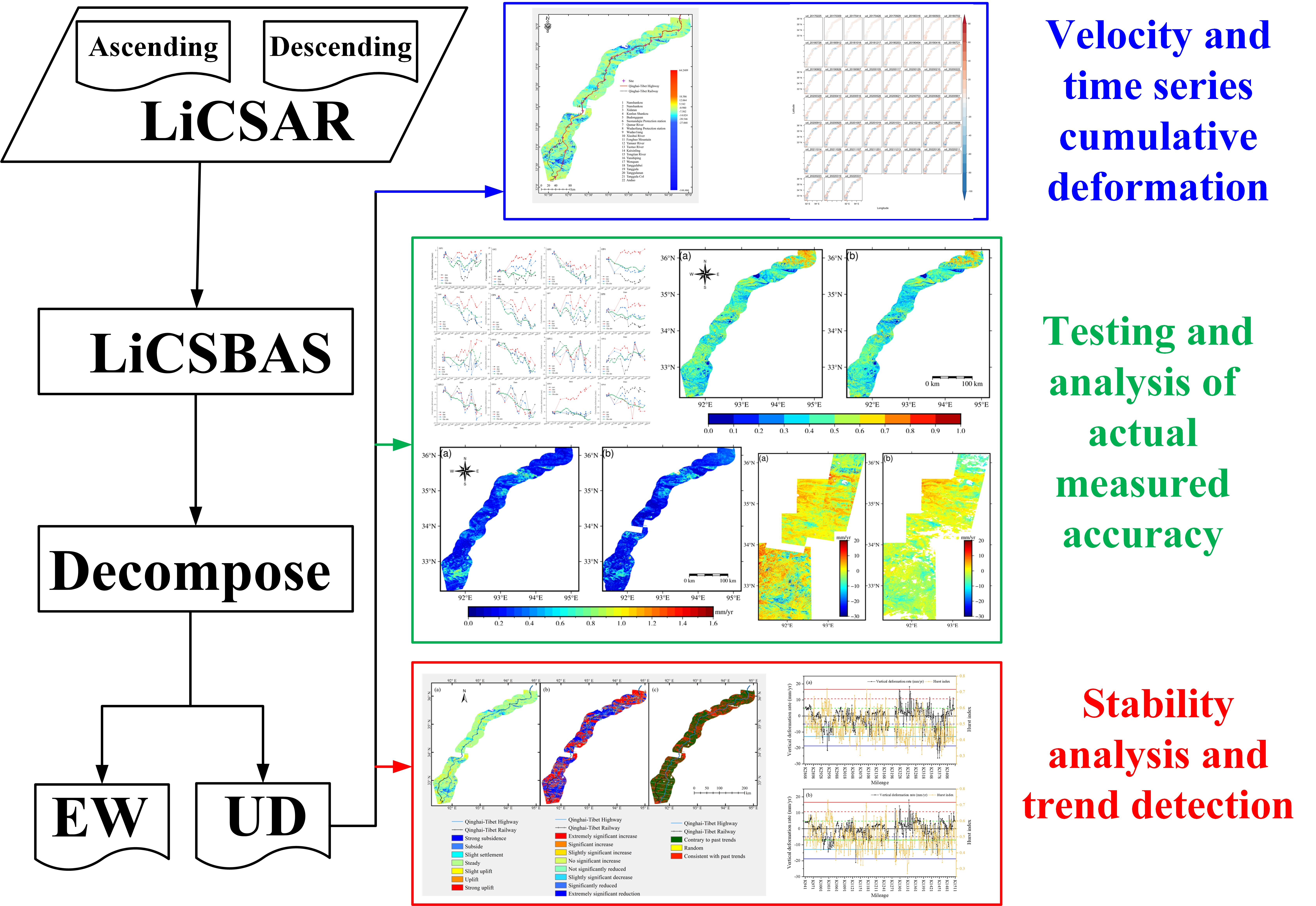
2. Study Area Overview
3. Materials and Methods
3.1. Surface Uplift or Settlement Calculation
3.2. Post-Processing Analysis of Results
3.2.1. Deformation Velocity Partitioning
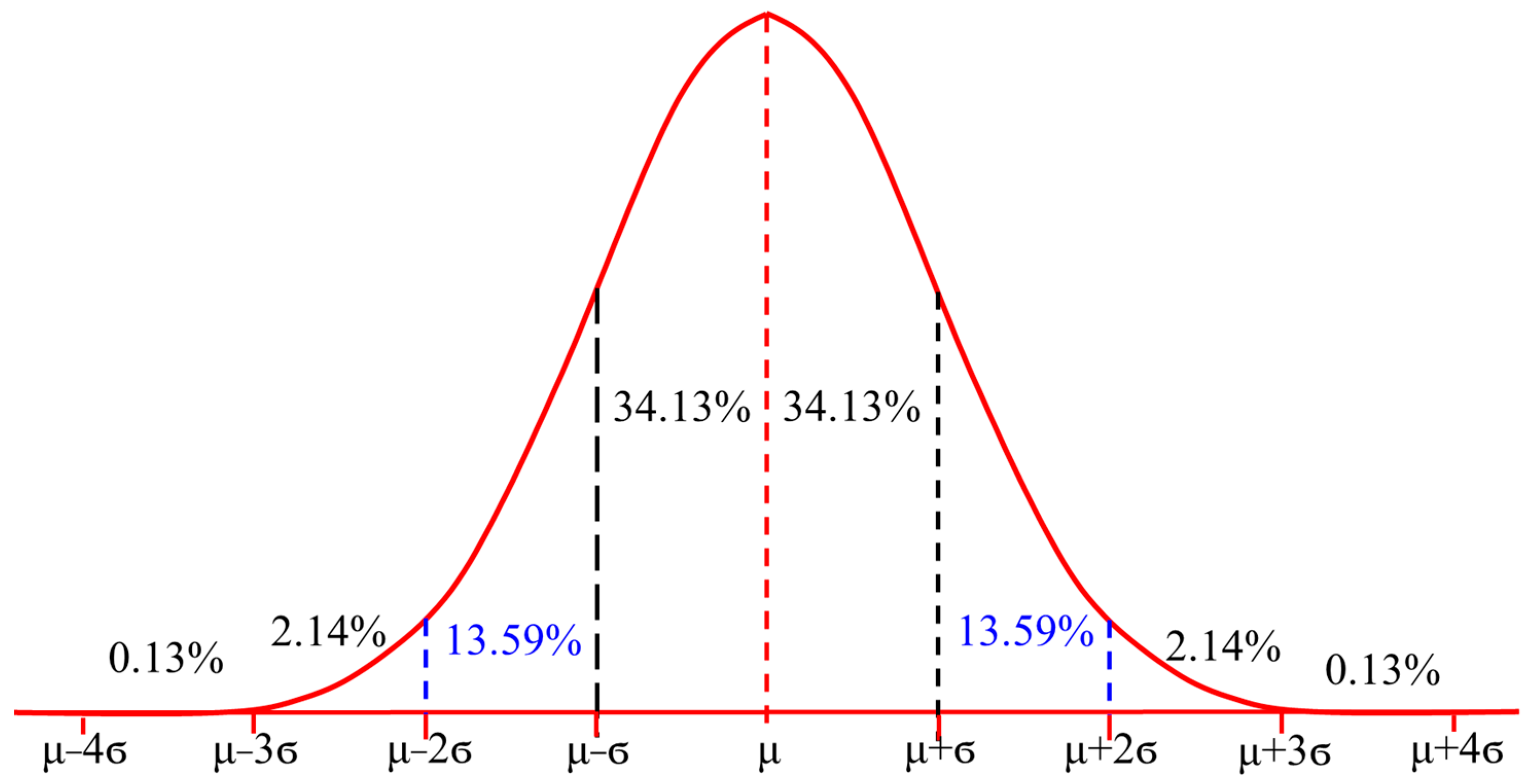
3.2.2. Cumulative Deformation Trend Detection and Significance Test
3.2.3. Trend Prediction of Surface Deformation Change
4. Results Analysis
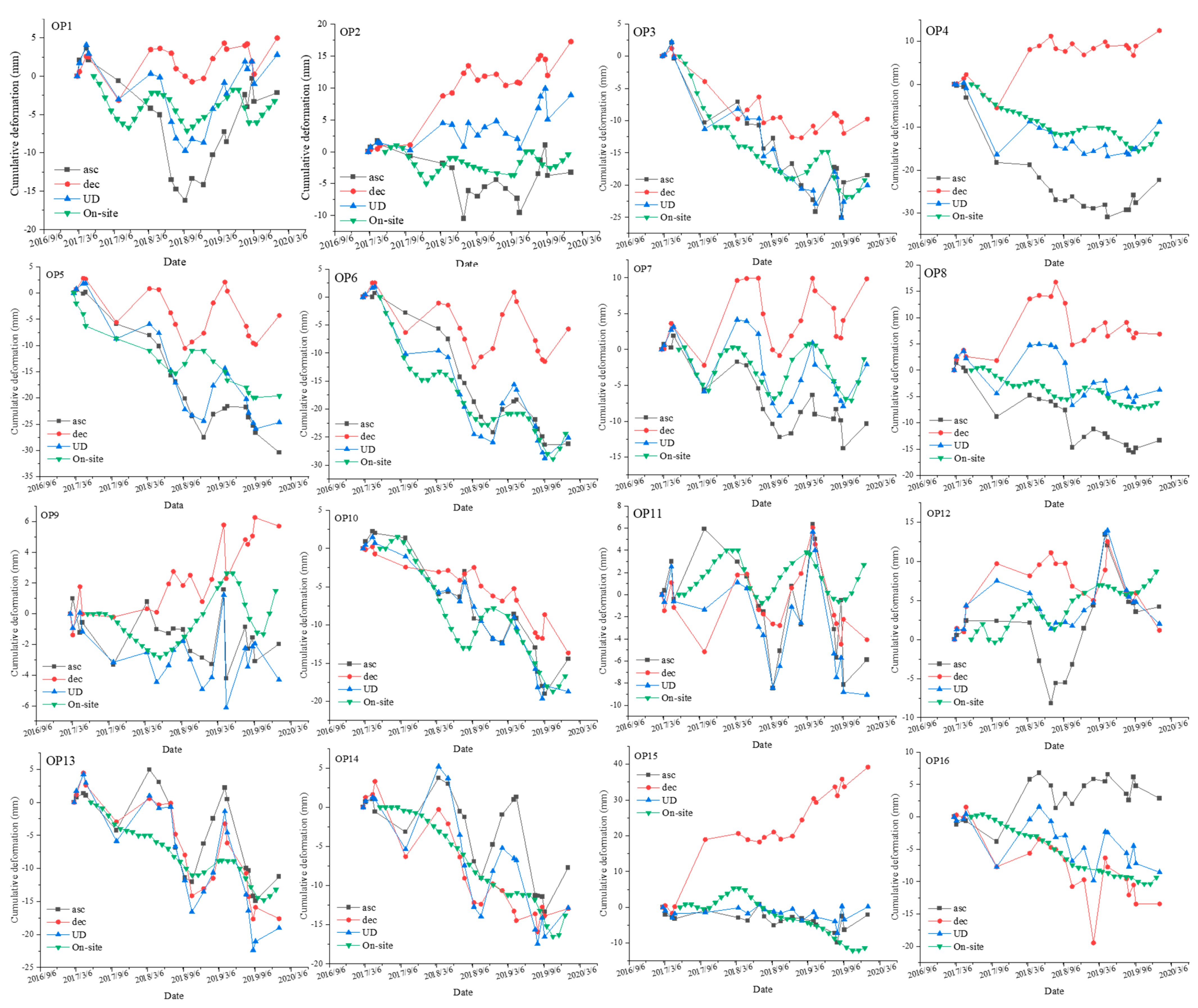
4.1. Results of the Accuracy Verification
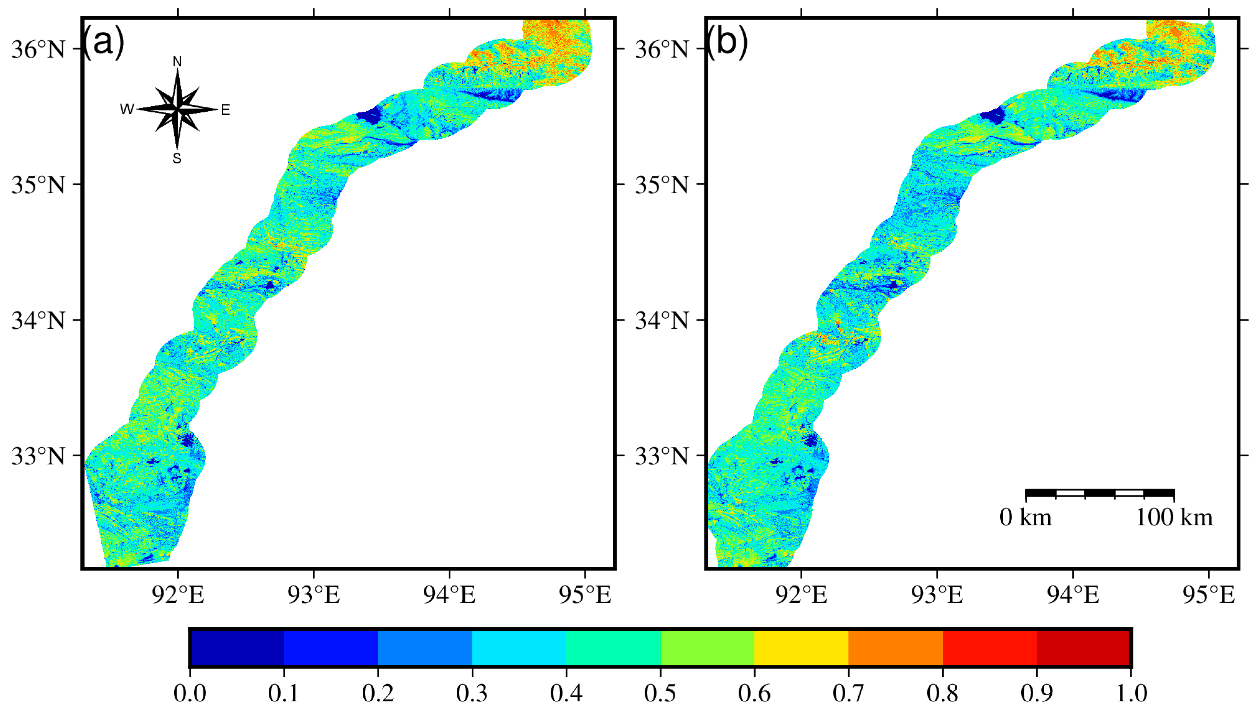
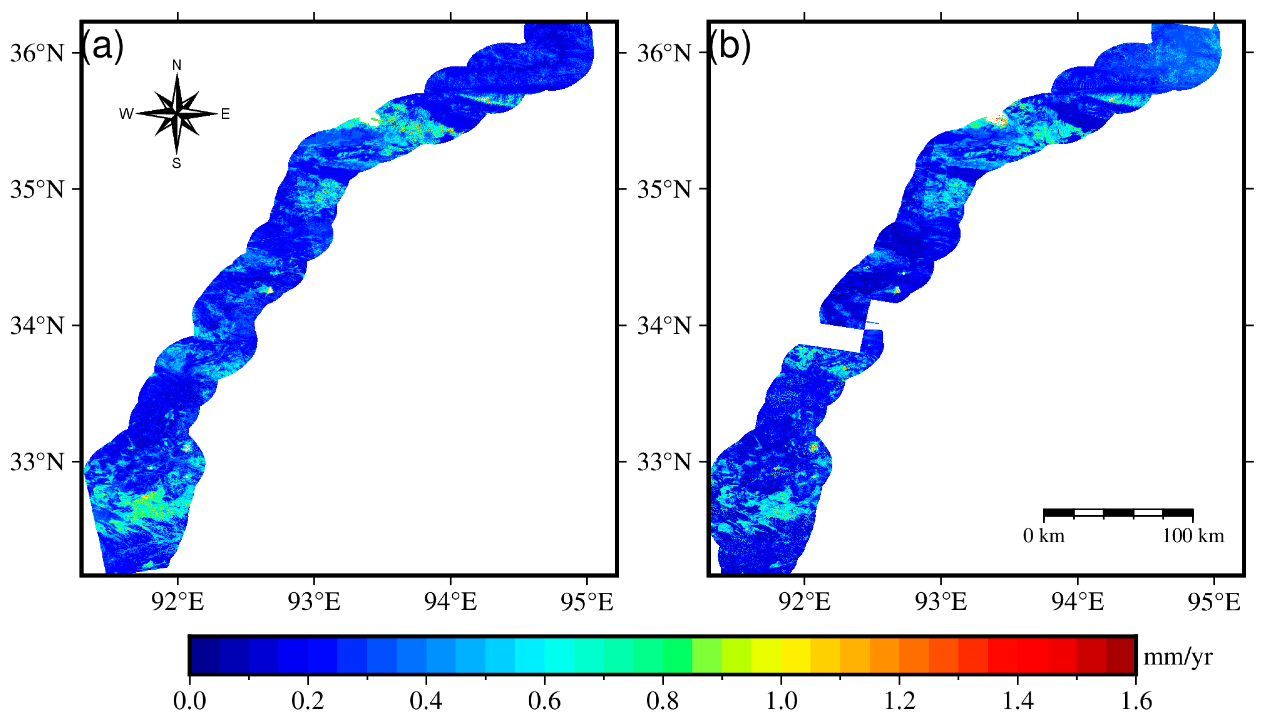
4.2. Characteristics of the Deformation Results
4.3. Surface Stability Evaluation and Early Warning
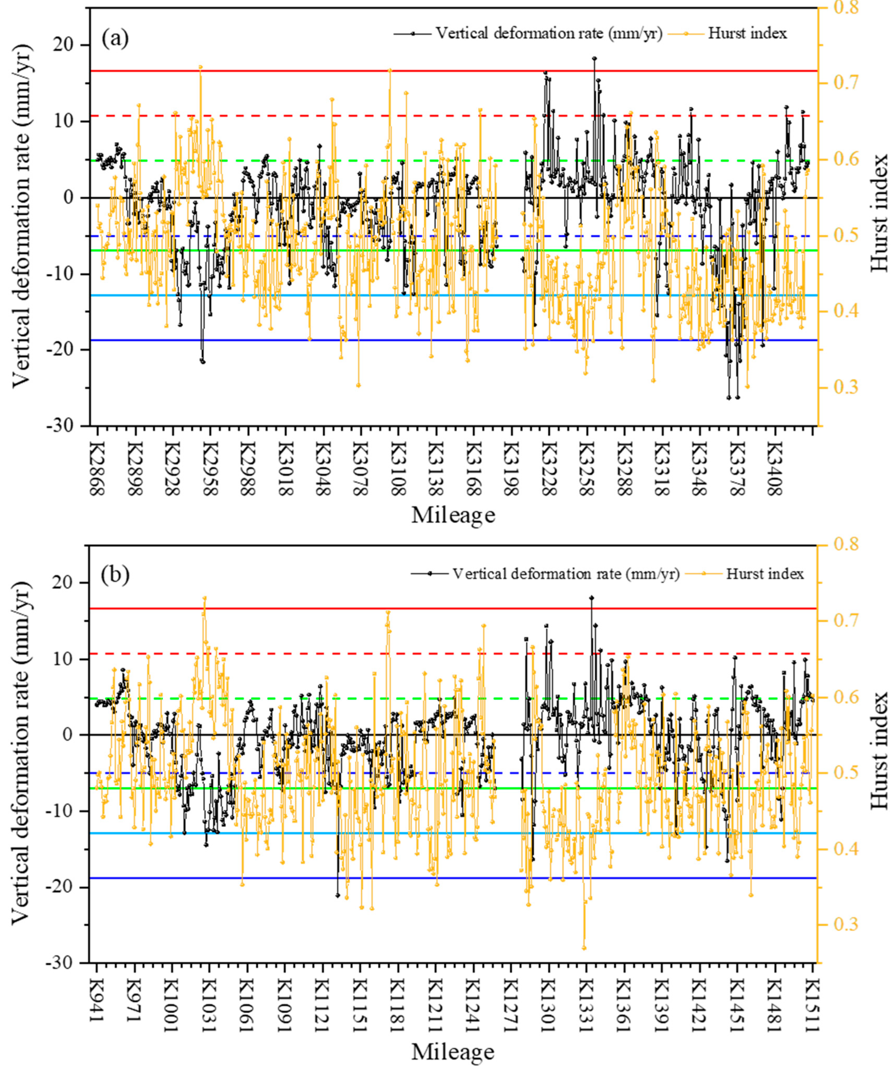
4.4. Linear Traffic Engineering Stability Evaluation and Early Warning
5. Discussion
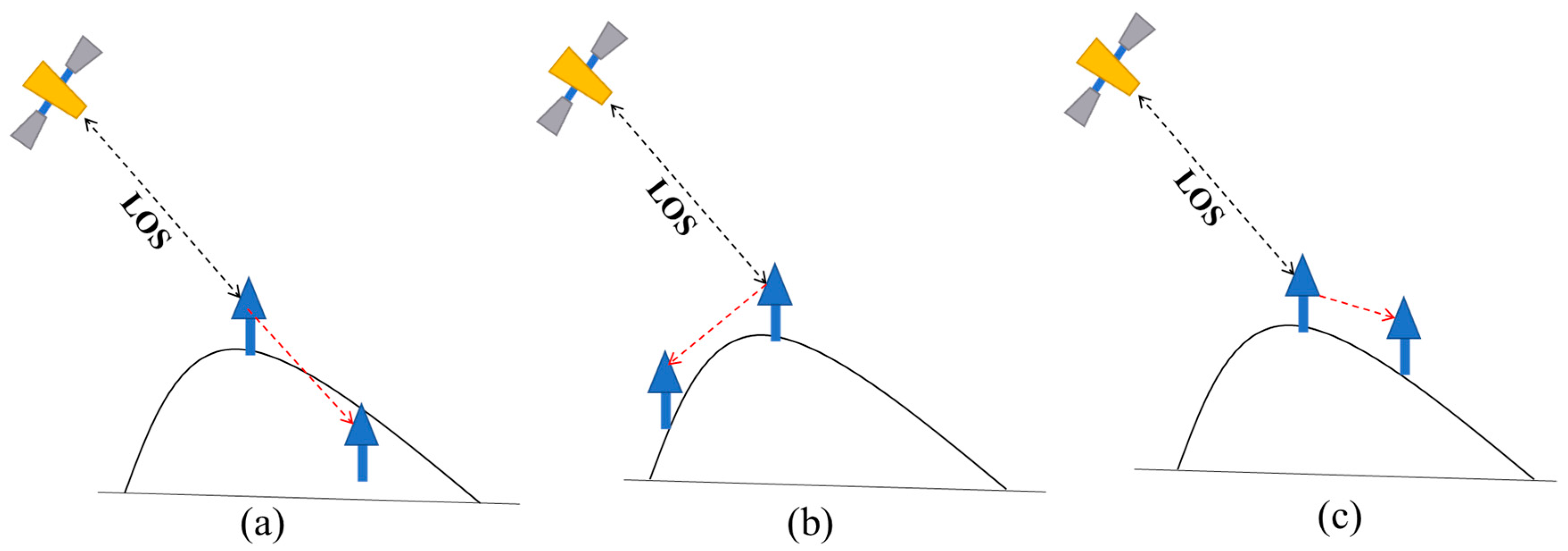
5.1. Necessity of Surface 2D Deformation InSAR Monitoring
5.2. Study of Surface Lift Driving Mechanism and Deformation Pattern
5.3. LiCSBAS Processing LiCSAR Results Applicability
6. Conclusions
- (1)
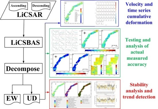
- Based on the LiCSAR product and LiCSBAS package, we can quickly obtain the surface deformation monitoring results of large-scale and long time series, and the calculations exhibit low consumption of computational resources, high computational efficiency, and the capability to be conducted in batch automation. It can also be used with other toolkits to quickly crop, mosaic, and select the deformation results for time periods of interest. This provides new methods and options for InSAR monitoring in the context of big data, cloud platforms, and cloud computing, and it lays a solid foundation for the development of large-scale surface deformation monitoring in the future.
- (2)
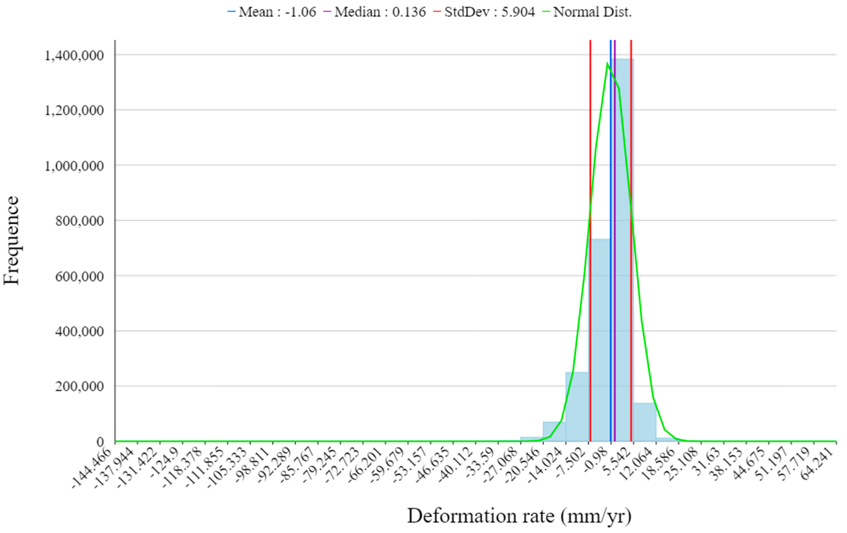
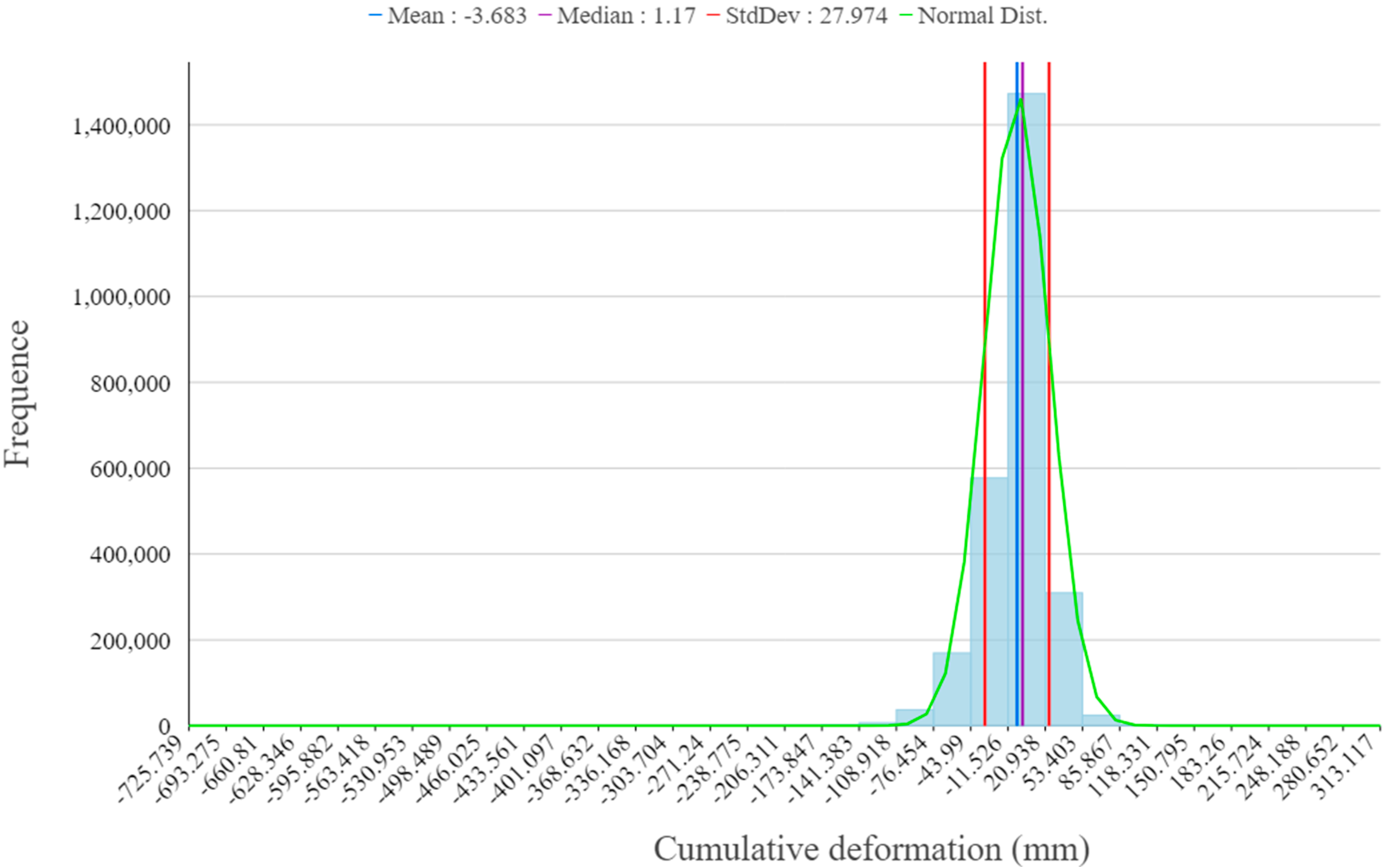
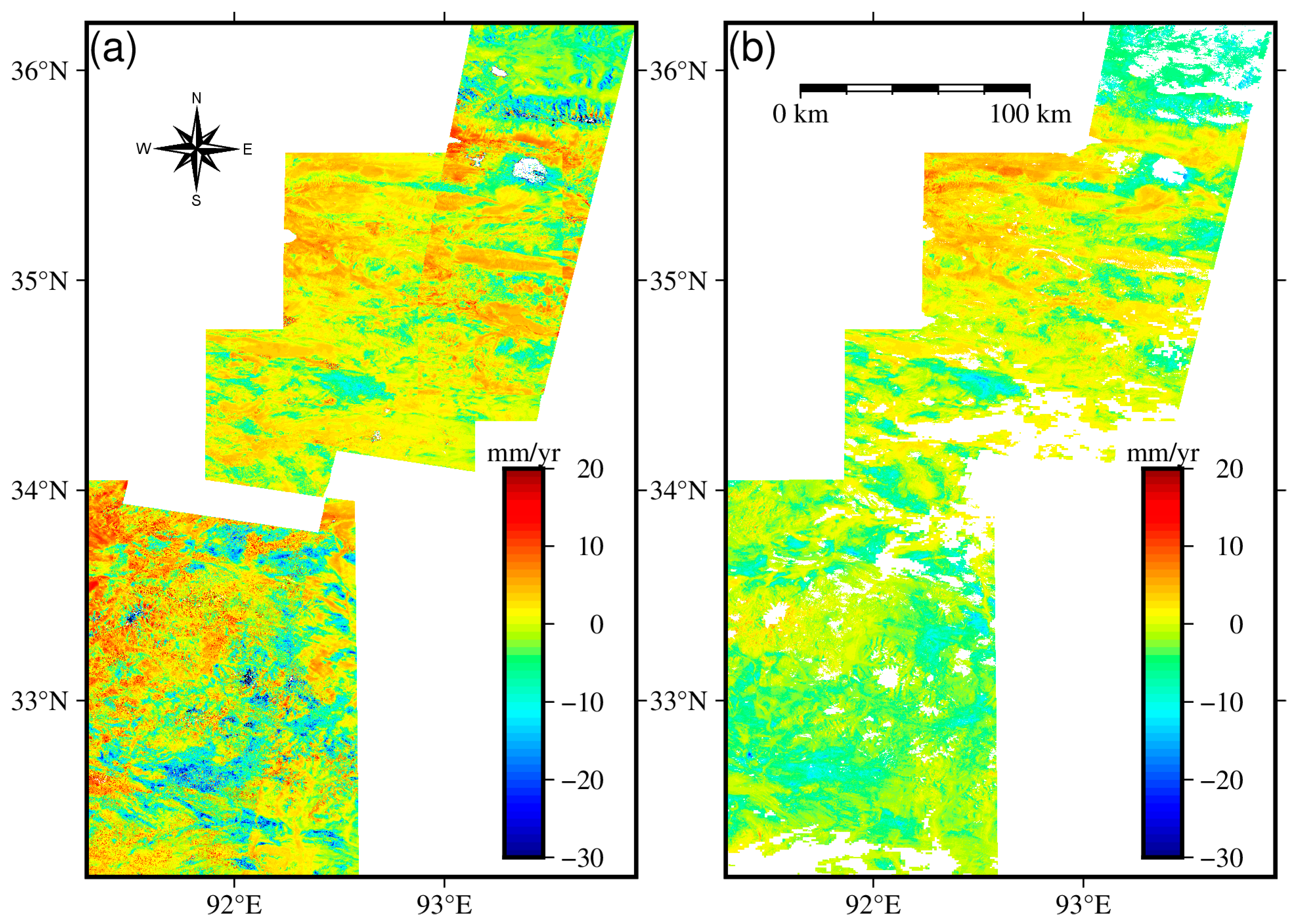
- The surface of the study area was in a slight settlement state from May 2017 to March 2022, and the vertical deformation rate was mostly distributed in the range of −27.068–18.586 mm/yr, with an average of −1.06 mm/yr. The results of the field monitoring show that the error of the vertical time series’ cumulative deformation was mostly less than 10 mm and the maximum was not more than 30 mm; while the error of the single ascending and descending track monitoring results was mostly more than 50 mm, and there are multiple deformation trend discrepancies. This shows that the vertical deformation results obtained using the same date or similar dates to obtain the deformation results for the ascending and descending tracks can better reflect the real settlement or uplift of the ground surface in the permafrost area.
- (3)
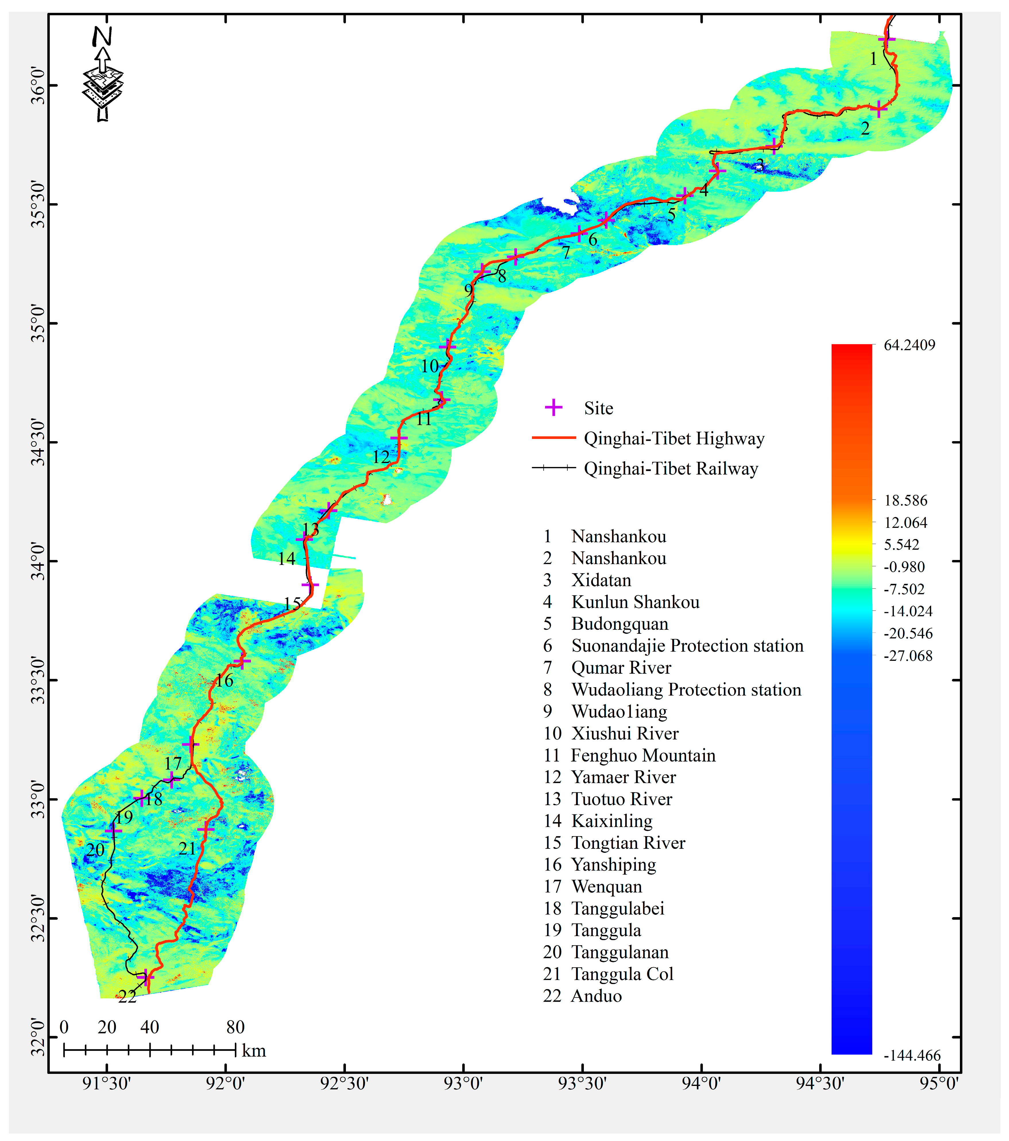
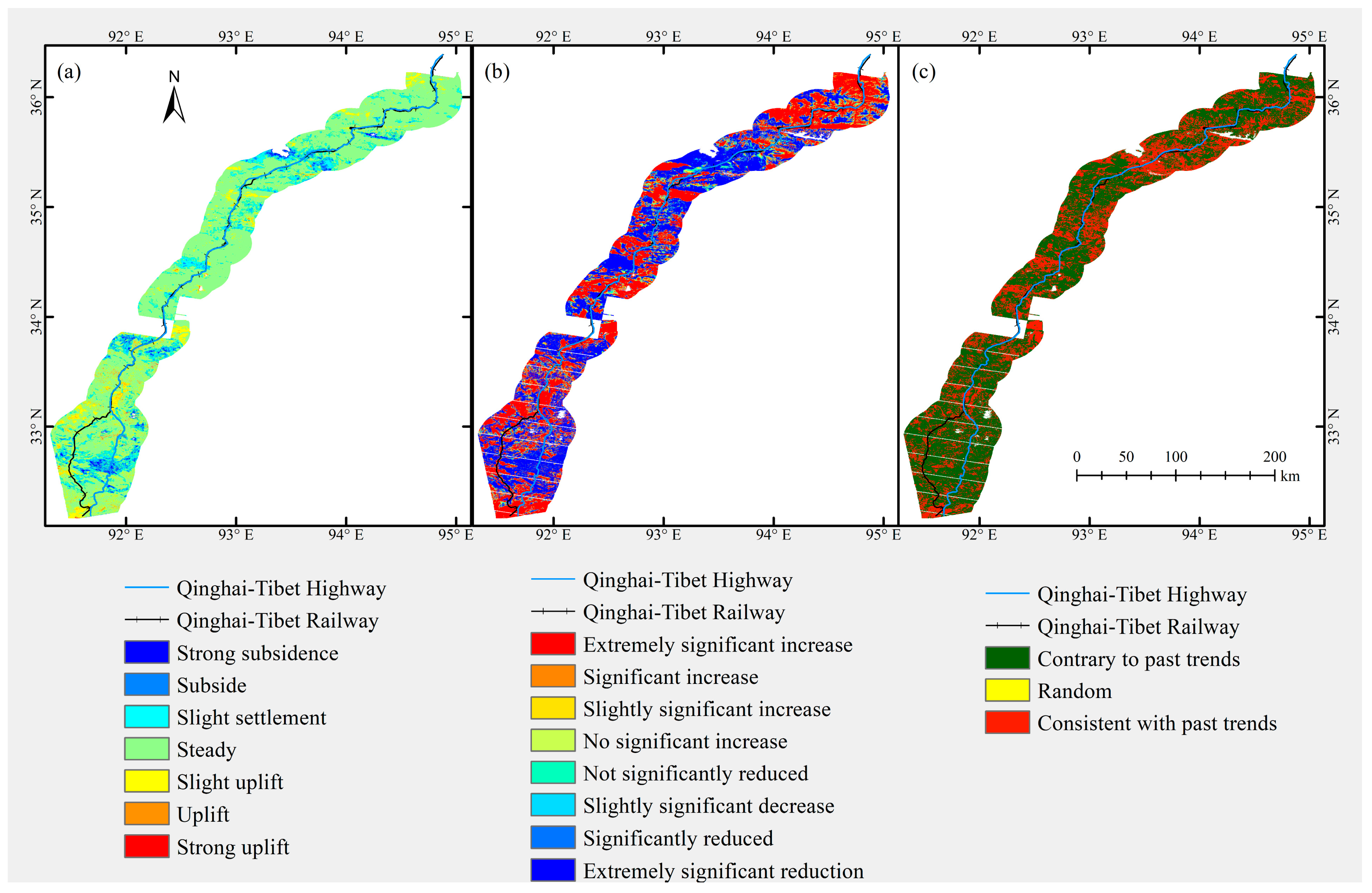
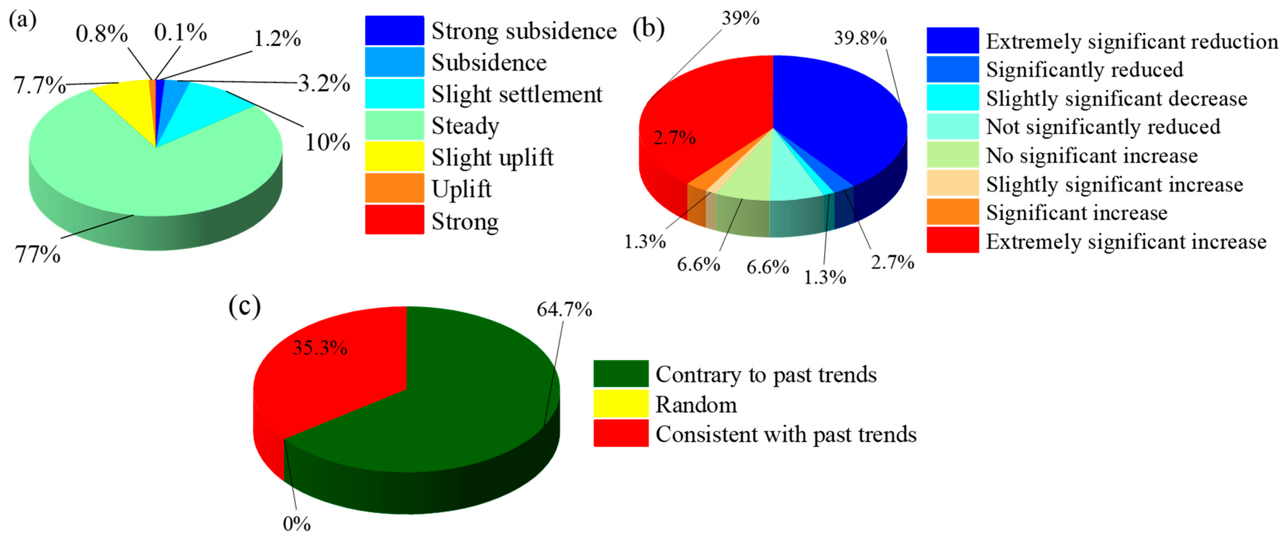
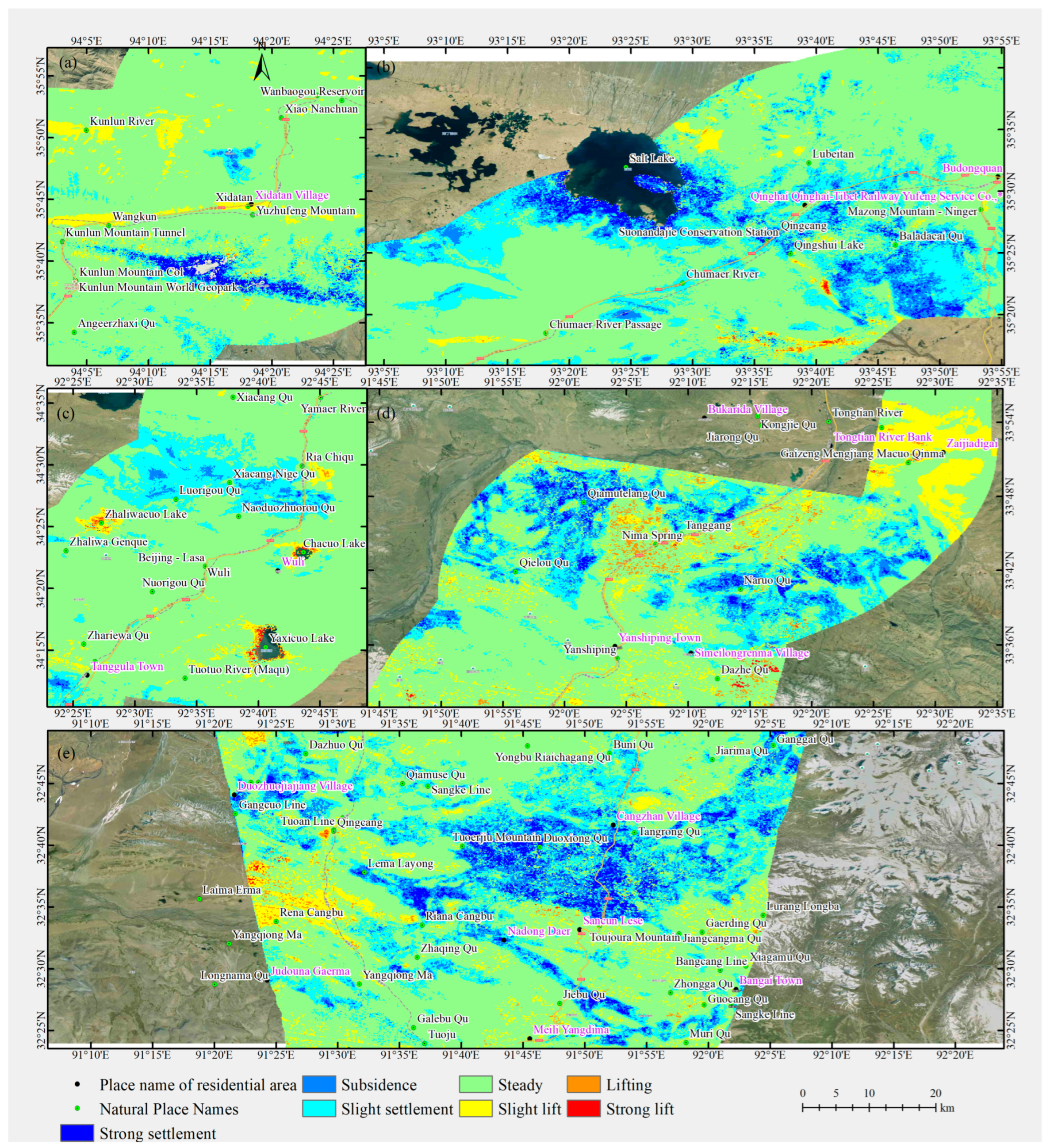
- A total of 77% of the engineering corridor was in a stable state, with vertical deformation rates between −6.964 mm/yr and 4.844 mm/yr, while 17.7% of the area was in a sub-stable state, wherein, 7.7% of the total area was considered unstable, including settlement rates between −12.868 mm/yr and −6.964 mm/yr, accounting for 10% of the total area, and the slightly uplifted area (uplift rate between 4.844 mm/yr and 10.748 mm/yr) accounting for 7.7% of the total area. The unstable area included an area with a settling rate greater than 12.868 mm/yr and an uplift rate greater than 10.748 mm/yr, accounting for 4.4% and 0.9% of the total area, respectively, totaling 5.3%. There were five large subsidence areas within the project corridor, containing numerous subsidence funnels, while the uplift areas were much smaller and sporadically distributed compared to the subsidence areas.
- (4)
- The stability of the areas along the Qinghai–Tibet Railway is significantly higher than that of the Qinghai–Tibet Highway, and there are fewer sections located in unstable areas. Four areas with serious settlement and one area with obvious uplift were found along the highway, while only two areas were found to be unstable along the railway, one each for settlement and uplift. The areas that need to be focused on in the future for the Qinghai–Tibet Highway are the five areas of subsidence and two areas of uplift, while the areas of subsidence and uplift along the railroad are areas two and one, respectively. The results obtained based on the method outlined in this paper can provide effective data support and the specific locations of high-risk areas for the safe operation of highways and railroads, as well as effective reference solutions for long-term monitoring and future early warning.
Supplementary Materials
Author Contributions
Funding
Data Availability Statement
Acknowledgments
Conflicts of Interest
Appendix A

References
- Qin, D.; Yao, T.; Ding, Y.; Ren, J. Glossary of Cryospheric Science; Revision 2; China Meteorological Press: Beijing, China, 2016; ISBN 978-7-5029-6473-3. [Google Scholar]
- Qin, D.; Yao, T.; Ding, Y.; Ren, J. Introduction to Cryspheric Science; Science Press: Beijing, China, 2018; ISBN 978-7-03-056573-0. [Google Scholar]
- Ran, Y.; Li, X.; Cheng, G.; Zhang, T.; Wu, Q.; Jin, H.; Jin, R. Distribution of Permafrost in China: An Overview of Existing Permafrost Maps. Permafr. Periglac. Process. 2012, 23, 322–333. [Google Scholar] [CrossRef]
- Zhou, Y.; Qiu, G.; Guo, D.; Cheng, G.; Li, S. Geocryology in China; Science Press: Beijing, China, 2000; ISBN 7-03-008285-0. [Google Scholar]
- Zhang, Z.; Lin, H.; Wang, M.; Liu, X.; Chen, Q.; Wang, C.; Zhang, H. A Review of Satellite Synthetic Aperture Radar Interferometry Applications in Permafrost Regions: Current Status, Challenges, and Trends. IEEE Geosci. Remote Sens. Mag. 2022, 10, 93–114. [Google Scholar] [CrossRef]
- Niu, F.; Yin, G.; Luo, J.; Lin, Z.; Liu, M. Permafrost Distribution along the Qinghai-Tibet Engineering Corridor, China Using High-Resolution Statistical Mapping and Modeling Integrated with Remote Sensing and GIS. Remote Sens. 2018, 10, 215. [Google Scholar] [CrossRef] [Green Version]
- Zhang, Z.; Wang, M.; Wu, Z.; Liu, X. Permafrost Deformation Monitoring Along the Qinghai-Tibet Plateau Engineering Corridor Using InSAR Observations with Multi-Sensor SAR Datasets from 1997–2018. Sensors 2019, 19, 5306. [Google Scholar] [CrossRef] [Green Version]
- Kriswati, E.; Agustan; Frederik, M.; Saepuloh, A.; Darmawan, S.; Alfianti, H. Long Term Ground Deformation of Mount Raung as Inferred by InSAR and GPS Data. In Proceedings of the 2021 7th Asia-Pacific Conference on Synthetic Aperture Radar (APSAR), New York, NY, USA, 1–3 November 2021. [Google Scholar]
- Qi, S.; Li, G.; Chen, D.; Chai, M.; Zhou, Y.; Du, Q.; Cao, Y.; Tang, L.; Jia, H. Damage Properties of the Block-Stone Embankment in the Qinghai–Tibet Highway Using Ground-Penetrating Radar Imagery. Remote Sens. 2022, 14, 2950. [Google Scholar] [CrossRef]
- Jia, S.; Zhang, T.; Fan, C.; Liu, L.; Shao, W. Research Progress of InSAR Technology in Permafrost. Adv. Earth Sci. 2021, 36, 694–711. [Google Scholar]
- Liu, S.; Zhao, L.; Wang, L.; Zou, D.; Zhou, H.; Xie, C.; Qiao, Y.; Yue, G.; Shi, J. Application of InSAR technology to monitor deformation in permafrost areas. J. Glaciol. Geocryol. 2021, 43, 964–975. [Google Scholar] [CrossRef]
- Du, Q.; Li, G.; Peng, W.; Zhou, Y.; Chai, M.; Li, J. Acquiring high-precision DEM in high altitude and cold area using InSAR technology. Bull. Surv. Mapp. 2021, 0, 44–49. [Google Scholar] [CrossRef]
- Zhao, T.; Zhang, M.; Pei, W.; Wang, J.; Yue, P.; Bi, J. Application of the differential interferometric synthetic aperture radar (D-InSAR) technology to monitor the ground surface deformation in permafrost regions. J. Glaciol. Geocryol. 2020, 42, 1087–1097. [Google Scholar] [CrossRef]
- Du, Q.; Li, G.; Zhou, Y.; Chen, D.; Chai, M.; Qi, S.; Cao, Y.; Tang, L.; Jia, H. Route Plans for UAV Aerial Surveys According to Different DEMs in Complex Mountainous Surroundings: A Case Study in the Zheduoshan Mountains, China. Remote Sens. 2022, 14, 5215. [Google Scholar] [CrossRef]
- Du, Q.; Li, G.; Chen, D.; Zhou, Y.; Qi, S.; Wu, G.; Chai, M.; Tang, L.; Jia, H.; Peng, W. SBAS-InSAR-Based Analysis of Surface Deformation in the Eastern Tianshan Mountains, China. Front. Earth Sci. 2021, 9, 729454. [Google Scholar] [CrossRef]
- Wang, J.; Wang, C.; Zhang, H.; Tang, Y.; Duan, W.; Dong, L. Freeze-Thaw Deformation Cycles and Temporal-Spatial Distribution of Permafrost along the Qinghai-Tibet Railway Using Multitrack InSAR Processing. Remote Sens. 2021, 13, 4744. [Google Scholar] [CrossRef]
- Li, G.; Zhao, C.; Wang, B.; Peng, M.; Bai, L. Evolution of Spatiotemporal Ground Deformation over 30 Years in Xi’an, China, with Multi-Sensor SAR Interferometry. J. Hydrol. 2023, 616, 128764. [Google Scholar] [CrossRef]
- Lin, S.-Y. Urban Hazards Caused by Ground Deformation and Building Subsidence over Fossil Lake Beds: A Study from Taipei City. Geomat. Nat. Hazards Risk 2022, 13, 2890–2910. [Google Scholar] [CrossRef]
- Luo, Q.; Li, J.; Zhang, Y. Monitoring Subsidence over the Planned Jakarta-Bandung (Indonesia) High-Speed Railway Using Sentinel-1 Multi-Temporal InSAR Data. Remote Sens. 2022, 14, 4138. [Google Scholar] [CrossRef]
- Zhang, S.; Fan, Q.; Niu, Y.; Qiu, S.; Si, J.; Feng, Y.; Zhang, S.; Song, Z.; Li, Z. Two-Dimensional Deformation Monitoring for Spatiotemporal Evolution and Failure Mode of Lashagou Landslide Group, Northwest China. Landslides 2023, 20, 447–459. [Google Scholar] [CrossRef]
- Nádudvari, Á. Using Radar Interferometry and SBAS Technique to Detect Surface Subsidence Relating to Coal Mining in Upper Silesia from 1993–2000 and 2003–2010. Environ. Socio-Econ. Stud. 2016, 4, 24–34. [Google Scholar] [CrossRef] [Green Version]
- Du, Q.; Li, G.; Zhou, Y.; Chai, M.; Chen, D.; Qi, S.; Wu, G. Deformation Monitoring in an Alpine Mining Area in the Tianshan Mountains Based on SBAS-InSAR Technology. Adv. Mater. Sci. Eng. 2021, 2021, 9988017. [Google Scholar] [CrossRef]
- Wang, Z.; Hu, J.; Chen, Y.; Liu, X.; Liu, J.; Wu, W.; Wang, Y. Integration of Ground-Based and Space-Borne Radar Observations for Three-Dimensional Deformations Reconstruction: Application to Luanchuan Mining Area, China. Geomat. Nat. Hazards Risk 2022, 13, 2819–2839. [Google Scholar] [CrossRef]
- Chang, M.; Sun, W.; Xu, H.; Tang, L. Identification and Deformation Analysis of Potential Landslides after the Jiuzhaigou Earthquake by SBAS-InSAR. Environ. Sci. Pollut. Res. Int. 2023, 30, 39093–39106. [Google Scholar] [CrossRef]
- Ramzan, U.; Fan, H.; Aeman, H.; Ali, M.; Al-qaness, M.A.A. Combined Analysis of PS-InSAR and Hypsometry Integral (HI) for Comparing Seismic Vulnerability and Assessment of Various Regions of Pakistan. Sci. Rep. 2022, 12, 22423. [Google Scholar] [CrossRef] [PubMed]
- Albino, F.; Biggs, J.; Lazecky, M.; Maghsoudi, Y. Routine Processing and Automatic Detection of Volcanic Ground Deformation Using Sentinel-1 InSAR Data: Insights from African Volcanoes. Remote Sens. 2022, 14, 5703. [Google Scholar] [CrossRef]
- Polcari, M.; Borgstrom, S.; Del Gaudio, C.; De Martino, P.; Ricco, C.; Siniscalchi, V.; Trasatti, E. Thirty Years of Volcano Geodesy from Space at Campi Flegrei Caldera (Italy). Sci. Data 2022, 9, 728. [Google Scholar] [CrossRef] [PubMed]
- Pourkhosravani, M.; Mehrabi, A.; Pirasteh, S.; Derakhshani, R. Monitoring of Maskun Landslide and Determining Its Quantitative Relationship to Different Climatic Conditions Using D-InSAR and PSI Techniques. Geomat. Nat. Hazards Risk 2022, 13, 1134–1153. [Google Scholar] [CrossRef]
- Dai, K.; Deng, J.; Xu, Q.; Li, Z.; Shi, X.; Hancock, C.; Wen, N.; Zhang, L.; Zhuo, G. Interpretation and Sensitivity Analysis of the InSAR Line of Sight Displacements in Landslide Measurements. Gisci. Remote Sens. 2022, 59, 1226–1242. [Google Scholar] [CrossRef]
- Feng, X.; Chen, Z.; Li, G.; Ju, Q.; Yang, Z.; Cheng, X. Improving the Capability of D-InSAR Combined with Offset-Tracking for Monitoring Glacier Velocity. Remote Sens. Environ. 2023, 285, 113394. [Google Scholar] [CrossRef]
- Ding, Y.; Liu, R.; Fan, Y.; Zhou, L.; Ji, Q.; Zhang, H.; Xiao, Z. Monitoring Glaciers in the Chenab Basin with SBAS InSAR Technology. J. Mt. Sci. 2022, 19, 2622–2633. [Google Scholar] [CrossRef]
- Liang, Q.; Wang, N. Mountain Glacier Flow Velocity Retrieval from Ascending and Descending Sentinel-1 Data Using the Offset Tracking and MSBAS Technique: A Case Study of the Siachen Glacier in Karakoram from 2017 to 2021. Remote Sens. 2023, 15, 2594. [Google Scholar] [CrossRef]
- Chen, J.; Wu, T.; Zou, D.; Liu, L.; Wu, X.; Gong, W.; Zhu, X.; Li, R.; Hao, J.; Hu, G.; et al. Magnitudes and Patterns of Large-Scale Permafrost Ground Deformation Revealed by Sentinel-1 InSAR on the Central Qinghai-Tibet Plateau. Remote Sens. Environ. 2022, 268, 112778. [Google Scholar] [CrossRef]
- Liu, L.; Schaefer, K.; Zhang, T.; Wahr, J. Estimating 1992-2000 Average Active Layer Thickness on the Alaskan North Slope from Remotely Sensed Surface Subsidence. J. Geophys. Res. Earth Surf. 2012, 117, F01005. [Google Scholar] [CrossRef]
- Liu, L.; Zhang, T.; Wahr, J. InSAR Measurements of Surface Deformation over Permafrost on the North Slope of Alaska. J. Geophys. Res. Earth Surf. 2010, 115, F03023. [Google Scholar] [CrossRef]
- Abe, T.; Iwahana, G.; Tadono, T.; Iijima, Y. Ground Surface Displacement After a Forest Fire Near Mayya, Eastern Siberia, Using InSAR: Observation and Implication for Geophysical Modeling. Earth Space Sci. 2022, 9, e2022EA002476. [Google Scholar] [CrossRef]
- Wang, J.; Li, C.; Li, L.; Huang, Z.; Wang, C.; Zhang, H.; Zhang, Z. InSAR Time-Series Deformation Forecasting Surrounding Salt Lake Using Deep Transformer Models. Sci. Total Environ. 2023, 858, 159744. [Google Scholar] [CrossRef] [PubMed]
- Gorelick, N.; Hancher, M.; Dixon, M.; Ilyushchenko, S.; Thau, D.; Moore, R. Google Earth Engine: Planetary-Scale Geospatial Analysis for Everyone. Remote Sens. Environ. 2017, 202, 18–27. [Google Scholar] [CrossRef]
- Dong, J.; Xiao, X.; Menarguez, M.A.; Zhang, G.; Qin, Y.; Thau, D.; Biradar, C.; Moore, B. Mapping Paddy Rice Planting Area in Northeastern Asia with Landsat 8 Images, Phenology-Based Algorithm and Google Earth Engine. Remote Sens. Environ. 2016, 185, 142–154. [Google Scholar] [CrossRef] [PubMed] [Green Version]
- Liu, X.; Hu, G.; Chen, Y.; Li, X.; Xu, X.; Li, S.; Pei, F.; Wang, S. High-Resolution Multi-Temporal Mapping of Global Urban Land Using Landsat Images Based on the Google Earth Engine Platform. Remote Sens. Environ. 2018, 209, 227–239. [Google Scholar] [CrossRef]
- Lazecký, M.; Spaans, K.; González, P.J.; Maghsoudi, Y.; Morishita, Y.; Albino, F.; Elliott, J.; Greenall, N.; Hatton, E.; Hooper, A.; et al. LiCSAR: An Automatic InSAR Tool for Measuring and Monitoring Tectonic and Volcanic Activity. Remote Sens. 2020, 12, 2430. [Google Scholar] [CrossRef]
- Morishita, Y.; Lazecky, M.; Wright, T.J.; Weiss, J.R.; Elliott, J.R.; Hooper, A. LiCSBAS: An Open-Source InSAR Time Series Analysis Package Integrated with the LiCSAR Automated Sentinel-1 InSAR Processor. Remote Sens. 2020, 12, 424. [Google Scholar] [CrossRef] [Green Version]
- Doin, M.-P.; Lodge, F.; Guillaso, S.; Jolivet, R.; Lasserre, C.; Ducret, G.; Grandin, R.; Pathier, E.; Pinel, V. Presentation of the Small Baseline NSBAS Processing Chain on a Case Example: The Etna Deformation Monitoring from 2003 to 2010 Using Envisat Data. In Proceedings of the FRINGE 2011 ESA Conference, Frascati, Italy, 19–23 September 2011. [Google Scholar]
- López-Quiroz, P.; Doin, M.-P.; Tupin, F.; Briole, P.; Nicolas, J.-M. Time Series Analysis of Mexico City Subsidence Constrained by Radar Interferometry. J. Appl. Geophys. 2009, 69, 1–15. [Google Scholar] [CrossRef]
- Jung, J.; Kim, D.; Park, S.-E. Correction of Atmospheric Phase Screen in Time Series InSAR Using WRF Model for Monitoring Volcanic Activities. IEEE Trans. Geosci. Remote Sens. 2013, 52, 2678–2689. [Google Scholar] [CrossRef]
- Yu, C.; Li, Z.; Penna, N.T.; Crippa, P. Generic Atmospheric Correction Model for Interferometric Synthetic Aperture Radar Observations. J. Geophys. Res. Solid Earth 2018, 123, 9202–9222. [Google Scholar] [CrossRef]
- Morishita, Y. Nationwide Urban Ground Deformation Monitoring in Japan Using Sentinel-1 LiCSAR Products and LiCSBAS. Prog. Earth Planet. Sci. 2021, 8, 6. [Google Scholar] [CrossRef]
- Tsironi, V.; Ganas, A.; Karamitros, I.; Efstathiou, E.; Koukouvelas, I.; Sokos, E. Kinematics of Active Landslides in Achaia (Peloponnese, Greece) through InSAR Time Series Analysis and Relation to Rainfall Patterns. Remote Sens. 2022, 14, 844. [Google Scholar] [CrossRef]
- Watson, A.R.; Elliott, J.R.; Walters, R.J. Interseismic Strain Accumulation Across the Main Recent Fault, SW Iran, From Sentinel-1 InSAR Observations. J. Geophys. Res. Solid Earth 2022, 127, e2021JB022674. [Google Scholar] [CrossRef]
- Ghorbani, Z.; Khosravi, A.; Maghsoudi, Y.; Mojtahedi, F.F.; Javadnia, E.; Nazari, A. Use of InSAR Data for Measuring Land Subsidence Induced by Groundwater Withdrawal and Climate Change in Ardabil Plain, Iran. Sci. Rep. 2022, 12, 13998. [Google Scholar] [CrossRef]
- Tavus, B.; Kocaman, S.; Nefeslioglu, H.A. Landslide Detection Using InSAR Time Series in the Kalekoy Dam Reservoir (Bingol, Turkiye). In Image and Signal Processing for Remote Sensing Xxviii, Proceedings of the SPIE Remote Sensing, Berlin, Germany, 5–6 September 2022; Bruzzone, L., Bovolo, F., Pierdicca, N., Eds.; Spie-Int Soc Optical Engineering: Bellingham, WA, USA, 2022; Volume 12267, p. 122670U. [Google Scholar]
- Xu, Z.; Jiang, L.; Niu, F.; Guo, R.; Huang, R.; Zhou, Z.; Jiao, Z. Monitoring Regional-Scale Surface Deformation of the Continuous Permafrost in the Qinghai-Tibet Plateau with Time-Series InSAR Analysis. Remote Sens. 2022, 14, 2987. [Google Scholar] [CrossRef]
- Ma, S.; Zhao, J.; Chen, J.; Zhang, S.; Dong, T.; Mei, Q.; Hou, X.; Liu, G. Ground Surface Freezing and Thawing Index Distribution in the Qinghai-Tibet Engineering Corridor and Factors Analysis Based on GeoDetector Technique. Remote Sens. 2023, 15, 208. [Google Scholar] [CrossRef]
- Li, Z.; Zhou, T.; Bu, Q. Soil and Water Conservation Measures and Preliminary Effect Analysis for the Golmud-Lhasa Section of the Qinghai-Tibet Railway. In Proceedings of the Third National Member Congress of the Chinese Society for Soil and Water Conservation, Beijing, China, January 2006; pp. 325–329. [Google Scholar]
- Wang, S.; Wang, Z.; Chen, J. Frozen Soil Environment and Expressway Layout of the Engineering Corridor on the Qinghai-Tibet Plateau; Shanghai Science and Technology Press: Shanghai, China, 2017; ISBN 978-7-5478-3822-8. [Google Scholar]
- Kang, S.; Xu, Y.; You, Q.; Fluegel, W.-A.; Pepin, N.; Yao, T. Review of Climate and Cryospheric Change in the Tibetan Plateau. Environ. Res. Lett. 2010, 5, 015101. [Google Scholar] [CrossRef]
- Yin, G.; Niu, F.; Lin, Z.; Luo, J.; Liu, M. Data-Driven Spatiotemporal Projections of Shallow Permafrost Based on CMIP6 across the Qinghai-Tibet Plateau at 1 Km(2) Scale. Adv. Clim. Change Res. 2021, 12, 814–827. [Google Scholar] [CrossRef]
- Yin, G.; Zheng, H.; Niu, F.; Luo, J.; Lin, Z.; Liu, M. Numerical Mapping and Modeling Permafrost Thermal Dynamics across the Qinghai-Tibet Engineering Corridor, China Integrated with Remote Sensing. Remote Sens. 2018, 10, 2069. [Google Scholar] [CrossRef] [Green Version]
- Wu, Q.; Zhang, T. Changes in Active Layer Thickness over the Qinghai-Tibetan Plateau from 1995 to 2007. J. Geophys. Res. Atmos. 2010, 115, D09107. [Google Scholar] [CrossRef]
- Sun, Z.-Z.; Ma, W.; Wu, G.-L.; Liu, Y.-Z.; Li, G.-Y. Permafrost Degradation along the Qinghai–Tibet Highway from 1995 to 2020. Adv. Clim. Change Res. 2023, 14, 248–254. [Google Scholar] [CrossRef]
- Zhou, D.; Zuo, X.; Xi, W.; Xiao, B.; Liu, X. The LiCSBAS method considering atmospheric errors and phase unwrapping errors in the detection of geological disasters in alpine valley region. Bull. Surv. Mapp. 2022, 0, 114–120,147. [Google Scholar] [CrossRef]
- Bechor, N.B.D.; Zebker, H.A. Measuring Two-Dimensional Movements Using a Single InSAR Pair. Geophys. Res. Lett. 2006, 33, L16311. [Google Scholar] [CrossRef] [Green Version]
- Cheng, C.; Shi, P.; Song, C.; Gao, J. Geographic big-data: A new opportunity for geography complexity study. Acta Geogr. Sin. 2018, 73, 1397–1406. [Google Scholar] [CrossRef]
- Sun, Q.; Xue, C.; Liu, J.; Liu, X.; Hong, Y.; Wu, C. Spatiotemporal association patterns between marine net primary production and environmental parameters in a view of data mining. Mar. Environ. Sci. 2020, 39, 340–347,352. [Google Scholar] [CrossRef]
- Xu, J. Mathematical Methods in Contemporary Geography, 3rd ed.; Higher Education Press: Beijing, China, 2017; ISBN 978-7-04-046632-4. [Google Scholar]
- He, P.; Bi, R.; Xu, L.; Wang, J.; Cao, C. Using geographical detection to analyze responses of vegetation growth to climate change in the Loess Pla-teau, China. J. Appl. Ecol. 2022, 33, 448–456. [Google Scholar] [CrossRef]
- Li, Y.; Ma, X.; Qi, G.; Wu, Y. Studies on Water Retention Function of Anhui Province Based on InVEST Model of Parameter Localization. Resour. Environ. Yangtze Basin 2022, 31, 313–325. [Google Scholar]
- Liu, J.; Wang, S.; Huang, Y. Effect of Climate Change on Runoff in a Basin with Mountain Permafrost, Northwest China. Permafr. Periglac. Process. 2007, 18, 369–377. [Google Scholar] [CrossRef]
- Hirsch, R.M.; Slack, J.R.; Smith, R.A. Techniques of Trend Analysis for Monthly Water Quality Data. Water Resour. Res. 1982, 18, 107–121. [Google Scholar] [CrossRef] [Green Version]
- Ghafouri-Azar, M.; Lee, S.-I. Meteorological Influences on Reference Evapotranspiration in Different Geographical Regions. Water 2023, 15, 454. [Google Scholar] [CrossRef]
- Lu, W. Spatial Distribution and Trend Prediction of Land Subsidence in Huhhot. Master’s Thesis, Inner Mongolia Normal University, Huhhot, China, June 2022. [Google Scholar]
- de Jong, R.; de Bruin, S.; de Wit, A.; Schaepman, M.E.; Dent, D.L. Analysis of Monotonic Greening and Browning Trends from Global NDVI Time-Series. Remote Sens. Environ. 2011, 115, 692–702. [Google Scholar] [CrossRef] [Green Version]
- Yin, Z.; Feng, Q.; Wang, L.; Chen, Z.; Chang, Y.; Zhu, R. Vegetation coverage change and its influencing factors across the northwest region of China during 2000–2019. J. Desert Res. 2022, 42, 11–21. [Google Scholar]
- Huang, H.; Xu, H.; Lin, T.; Xia, G. Spatio-temporal variation characteristics of NDVI and its response to climate change in the Altay region of Xinjiang from 2001 to 2020. Acta Ecol. Sin. 2022, 42, 2798–2809. [Google Scholar] [CrossRef]
- Wang, Y.-Z.; Li, B.; Wang, R.-Q.; Su, J.; Rong, X.-X. Application of the Hurst Exponent in Ecology. Comput. Math. Appl. 2011, 61, 2129–2131. [Google Scholar] [CrossRef] [Green Version]
- Alvo, M.; Theberge, F. Hurst Exponents for Non-Precise Data. Iran. J. Fuzzy Syst. 2013, 10, 73–81. [Google Scholar]
- Yan, E.; Lin, H.; Dang, Y.; Xia, C. The spatiotemporal changes of vegetation cover in Beijing-Tianjin sandstorm source control region during 2000–2012. Acta Ecol. Sin. 2014, 34, 5007–5020. [Google Scholar] [CrossRef] [Green Version]
- Li, X.; Yang, D.; Feng, L.; Huang, Y.; Yi, W. Dynamics of vegetation NDVI in Chengdu-Chongqing Economic Circle from 2000 to 2018. Chin. J. Ecol. 2021, 40, 2967–2977. [Google Scholar] [CrossRef]
- Hu, J.; Li, Z.; Zhu, J.; Liu, J. Theory and Application of Monitoring 3-D Deformation with InSAR; Science Press: Beijing, China, 2021; ISBN 978-7-03-068643-5. [Google Scholar]
- Hu, J. Theory and Method of Estimating Three-Dimensional Displacement with InSAR Based on the Modern Surveying Adjustment. Ph.D. Thesis, Central South University, Changsha, China, December 2012. [Google Scholar]
- Wright, T.J.; Parsons, B.E.; Lu, Z. Toward Mapping Surface Deformation in Three Dimensions Using InSAR. Geophys. Res. Lett. 2004, 31. [Google Scholar] [CrossRef] [Green Version]
- Rocca, F. 3D Motion Recovery with Multi-Angle and/or Left Right Interferometry. In Proceedings of the FRINGE 2003 Workshop (ESA SP-550), Frascati, Italy, 1–5 December 2003. [Google Scholar]
- Joughin, I.R.; Kwok, R.; Fahnestock, M.A. Interferometric Estimation of Three-Dimensional Ice-Flow Using Ascending and Descending Passes. IEEE Trans. Geosci. Remote Sens. 1998, 36, 25–37. [Google Scholar] [CrossRef] [Green Version]
- Zhao, R.; Li, Z.; Feng, G.; Wang, Q.; Hu, J. Monitoring Surface Deformation over Permafrost with an Improved SBAS-InSAR Algorithm: With Emphasis on Climatic Factors Modeling. Remote Sens. Environ. 2016, 184, 276–287. [Google Scholar] [CrossRef]
- Zhao, T.; Zhang, M.; Lu, J.; Yan, Z. Correlation between ground surface deformation and influential factors in permafrost regions. J. Harbin Inst. Technol. 2021, 53, 145–153. [Google Scholar] [CrossRef]
- Wu, Y.; Liu, C.; Zhang, Q.; Ge, L. Bibliometric Analysis of Interferometric Synthetic Aperture Radar (InSAR) Application in Land Subsidence from 2000 to 2021. J. Sens. 2022, 2022, 1027673. [Google Scholar] [CrossRef]
- Efron, B.; Tibshirani, R. Bootstrap Methods for Standard Errors, Confidence Intervals, and Other Measures of Statistical Accuracy. Stat. Sci. 1986, 1, 54–75. [Google Scholar] [CrossRef]


| Area One | Areas Two, Three, and Four | Area One | Areas Two, Three, and Four | Area One | Areas Two, Three, and Four |
|---|---|---|---|---|---|
| 20 February 2017 | 25 February 2017 | 21 August 2019 | 26 August 2019 | 2 October 2020 | 7 October 2020 |
| 4 March 2017 | 9 March 2017 | 2 September 2019 | 7 September 2019 | 14 October 2020 | 19 October 2020 |
| 9 September 2017 | 14 April 2017 | 13 December 2019 | 5 January 2020 | 26 October 2020 | 31 October 2020 |
| 21 April 2017 | 26 April 2017 | 12 January 2020 | 17 January 2020 | 11 February 2021 | 16 February 2021 |
| 24 April 2017 | 29 September 2017 | 24 January 2020 | 29 January 2020 | 22 August 2021 | 27 August 2021 |
| 11 March 2018 | 16 March 2018 | 5 February 2020 | 10 February 2020 | 3 September 2021 | 8 September 2021 |
| 28 April 2018 | 3 May 2018 | 17 February 2020 | 22 February 2020 | 9 October 2021 | 14 October 2021 |
| 27 June 2018 | 2 July 2018 | 24 March 2020 | 29 March 2020 | 21 October 2021 | 26 October 2021 |
| 21 July 2018 | 26 July 2018 | 5 April 2020 | 10 April 2020 | 2 November 2021 | 7 November 2021 |
| 7 September 2018 | 12 September 2018 | 11 May 2020 | 16 May 2020 | 26 November 2021 | 1 December 2021 |
| 13 October 2018 | 18 October 2018 | 23 May 2020 | 28 May 2020 | 8 December 2021 | 13 December 2021 |
| 12 December 2018 | 17 December 2018 | 16 June 2020 | 21 June 2020 | 1 January 2022 | 6 January 2022 |
| 29 January 2019 | 3 February 2019 | 28 June 2020 | 3 July 2020 | 25 January 2022 | 30 January 2022 |
| 30 March 2019 | 4 April 2019 | 15 August 2020 | 20 August 2020 | 6 February 2022 | 11 February 2022 |
| 11 April 2019 | 16 April 2019 | 27 August 2020 | 1 September 2020 | 18 February 2022 | 23 February 2022 |
| 16 July 2019 | 21 July 2019 | 8 September 2020 | 13 September 2020 | 14 March 2022 | 19 March 2022 |
| 28 July 2019 | 2 August 2019 | 20 September 2020 | 25 September 2020 | 26 March 2022 | 31 March 2022 |
| Workflow | Step | Description | Parameters |
|---|---|---|---|
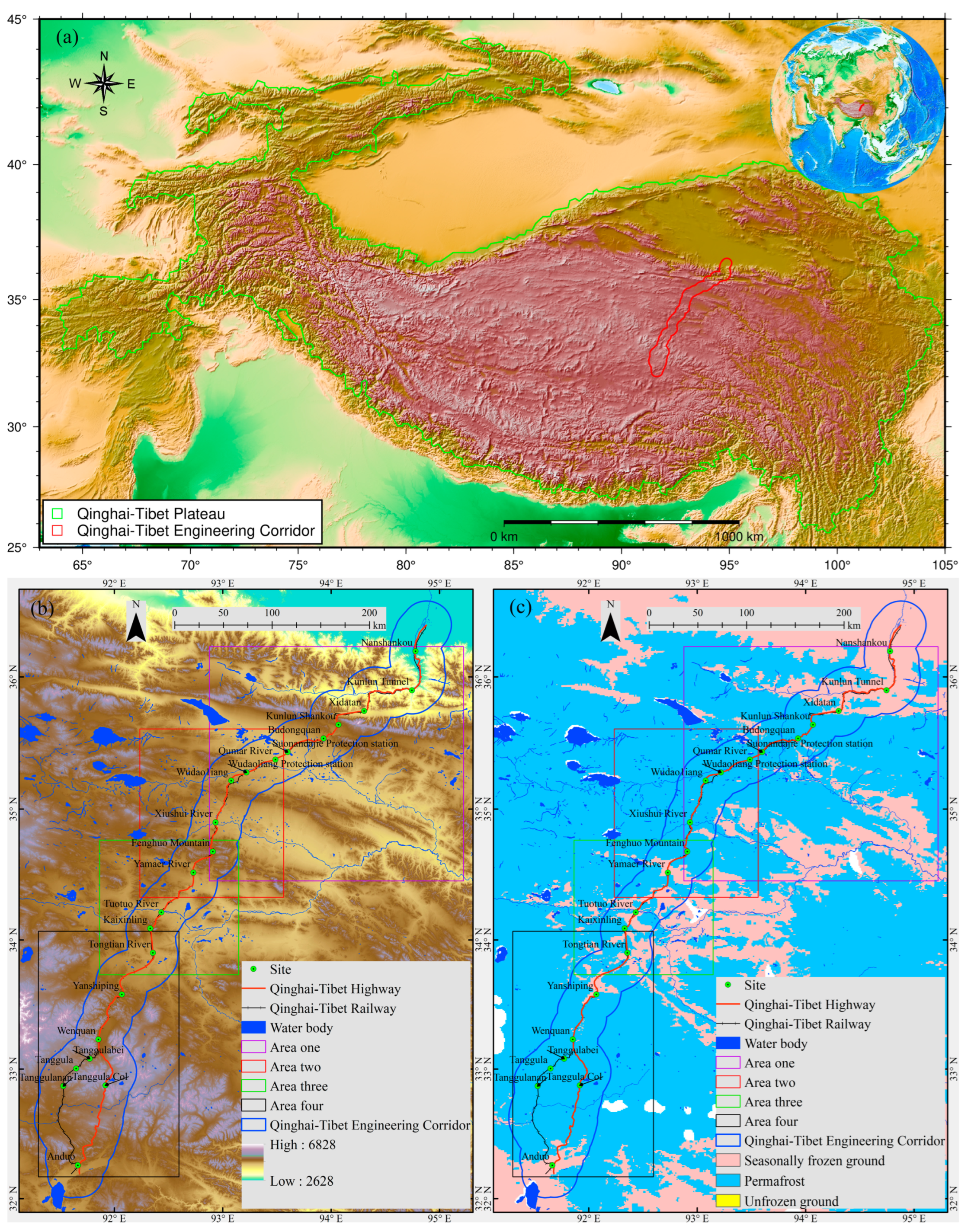
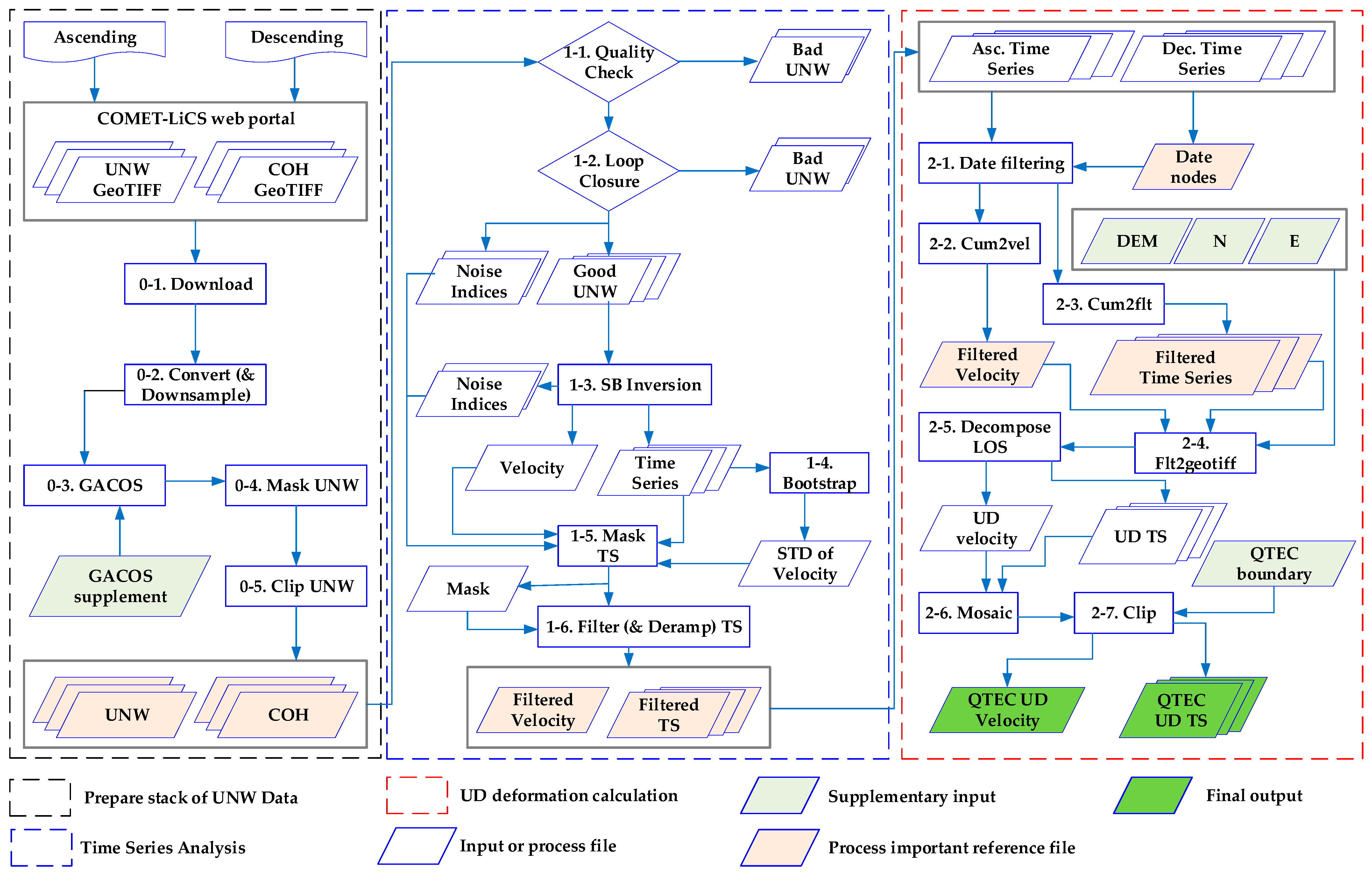
| Prepare stack of UNW Data | 0-1. Download | Retrieving GeoTIFF files of UNW from the COMET-LiCS web portal based on the frame ID | -f: Frame ID, -s: 20141001, -e: 20220331, --get_gacos: y, --n_para: 12 |
| 0-2. Convert (and Downsample) | Converting the GeoTIFF files of UNW and COH to float32 and uint8 formats, respectively | -n: 1, --n_para: 12 | |
| 0-3. GACOS | Applying a tropospheric correction to the UNW data using GACOS data | -g: Path to the dir containing all GACOS data, --n_para: 12 | |
| 0-4. Mask UNW | Masking specified areas or areas with low coherence in the UNW data | -c: 0.2, --n_para: 12 | |
| 0-5. Clip UNW | Clipping a specified rectangular area of interest from the unw and cc data | -g: 92.87/95.23/34.45/36.23 (area one), --n_para: 12 | |
| Time Series Analysis | 1-1. Quality Check | Assessing the quality of the UNW data and identifying bad interferograms based on average coherence and coverage | -c: 0.05, -u: 0.3 |
| 1-2. Loop Closure | Identifying bad UNW by checking loop closure and determining a preliminary reference point that contains all valid UNW data and exhibits the smallest RMS of loop phases | -l: 1.5 rad, --n_para: 12 | |
| 1-3. SB Inversion | Inverting the SB network of UNW to obtain the time series cumulative deformation and velocity using the NSBAS approach | --n_unw_r_thre: 1, --gpu: y | |
| 1-4. Bootstrap | Calculating the standard deviation of the velocity using the bootstrap method and STC | --mem_size: 8000, --gpu: y | |
| 1-5. Mask TS | Creating a mask for the time series deformation using several noise indices | -c: 0.05, -u: 1.5, -v: 100, -T: 1, -g: 10, -s: 5, -i: 50, -l: 5, -r: 2 | |
| 1-6. Filter (and Deramp) TS | Applying a spatio-temporal filter (high-pass in time and low-pass in space) with a Gaussian kernel, similar to StaMPS | -s: 1, -r: 2, --hgt_linea: y | |
| UD deformation calculation | 2-1. Date filtering | Filtering the measurement area with both ascending and descending orbital deformation time points | Implementation through R language conditional functions |
| 2-2. Cum2vel | Calculating the velocity and its standard deviation from the cumulative deformation of the time series | -s: 20170225, -e: 20220331, --vstd: y | |
| 2-3. Cum2flt | Generating a float32 file that represents the cumulative displacement over a specified date period derived from the original time series cumulative deformation | -d: each of the date notes, -m: 20170225 | |
| 2-4. Flt2geotiff | Converting the filtered velocity and time series cumulative deformation results from a float32 format image file to a GeoTIFF file | --a_nodata: −9999 | |
| 2-5. Decompose LOS | Decomposing 2 (or more) LOS displacement data into EW and UD components, assuming no displacement in the NS direction | -f: Text file containing input GeoTIFF file paths of LOS displacement (or velocity), E component, and N component (Format: dispfile1 Efile1 Nfile1 dispfile2 Efile2 Nfile2…), -r: cubic | |
| 2-6. Mosaic | Consolidating multiple raster datasets into a new raster dataset, such as the velocity and cumulative deformation results | mosaic operator: mean | |
| 2-7. Clip | Extracting a portion of the mosaic velocity and cumulative deformation based on the boundary (*.shp data) of the Qinghai Tibet Engineering Corridor | use input features for clipping geometry: yes |
| β | Z | Trend Characteristic |
|---|---|---|
| β > 0 | Z > 2.58 | Extremely significant increase |
| 1.96 < Z ≤ 2.58 | Significant increase | |
| 1.65 < Z ≤ 1.96 | Microsignificant increase | |
| Z ≤ 1.65 | No significant increase | |
| β = 0 | Z | No change |
| β < 0 | Z ≤ 1.65 | No significant reduction |
| 1.65 < Z ≤ 1.96 | Slightly significant reduction | |
| 1.96 < Z ≤ 2.58 | Significant reduction | |
| Z > 2.58 | Extremely significant reduction |
| Observation Sites | Longitude (E) | Latitude (N) | UD Deformation Rate | Asc. LOS Deformation Rate | Des. LOS Deformation Rate |
|---|---|---|---|---|---|
| OP1 | 94°03.081′ | 35°37.020′ | −0.769 | −3.331 | 1.795 |
| OP2 | 93°57.795′ | 35°33.109′ | 1.046 | −2.941 | 4.818 |
| OP3 | 93°43.561′ | 35°30.132′ | −7.807 | −8.141 | −1.896 |
| OP4 | 93°34.098′ | 35°24.548′ | −3.664 | −7.398 | 2.993 |
| OP5 | 93°26.776′ | 35°21.839′ | −8.299 | −10.236 | −1.760 |
| OP6 | 93°26.678′ | 35°21.819′ | −8.516 | −10.558 | −1.690 |
| OP7 | 93°06.678′ | 35°12.258′ | −2.244 | −3.813 | 1.442 |
| OP8 | 93°02.521′ | 35°08.303′ | −3.599 | −4.759 | −1.312 |
| OP9 | 92°53.914′ | 34°40.346′ | −0.419 | −0.476 | 2.700 |
| OP10 | 92°44.608′ | 34°34.532′ | −6.525 | −5.204 | −4.624 |
| OP11 | 92°43.568′ | 34°28.656′ | −2.019 | −2.704 | 0.163 |
| OP12 | 92°25.838′ | 34°12.968′ | −0.999 | 2.308 | −2.960 |
| OP13 | 92°20.386′ | 34°00.675′ | −6.992 | −4.581 | −6.343 |
| OP14 | 92°14.064′ | 33°46.399′ | −6.570 | −4.333 | −5.852 |
| OP15 | 91°56.752′ | 33°23.874′ | −1.828 | −2.628 | 9.093 |
| OP16 | 91°45.164′ | 33°04.292′ | −2.527 | 1.334 | −4.150 |
Disclaimer/Publisher’s Note: The statements, opinions and data contained in all publications are solely those of the individual author(s) and contributor(s) and not of MDPI and/or the editor(s). MDPI and/or the editor(s) disclaim responsibility for any injury to people or property resulting from any ideas, methods, instructions or products referred to in the content. |
© 2023 by the authors. Licensee MDPI, Basel, Switzerland. This article is an open access article distributed under the terms and conditions of the Creative Commons Attribution (CC BY) license (https://creativecommons.org/licenses/by/4.0/).
Share and Cite
Du, Q.; Chen, D.; Li, G.; Cao, Y.; Zhou, Y.; Chai, M.; Wang, F.; Qi, S.; Wu, G.; Gao, K.; et al. Preliminary Study on InSAR-Based Uplift or Subsidence Monitoring and Stability Evaluation of Ground Surface in the Permafrost Zone of the Qinghai–Tibet Engineering Corridor, China. Remote Sens. 2023, 15, 3728. https://doi.org/10.3390/rs15153728
Du Q, Chen D, Li G, Cao Y, Zhou Y, Chai M, Wang F, Qi S, Wu G, Gao K, et al. Preliminary Study on InSAR-Based Uplift or Subsidence Monitoring and Stability Evaluation of Ground Surface in the Permafrost Zone of the Qinghai–Tibet Engineering Corridor, China. Remote Sensing. 2023; 15(15):3728. https://doi.org/10.3390/rs15153728
Chicago/Turabian StyleDu, Qingsong, Dun Chen, Guoyu Li, Yapeng Cao, Yu Zhou, Mingtang Chai, Fei Wang, Shunshun Qi, Gang Wu, Kai Gao, and et al. 2023. "Preliminary Study on InSAR-Based Uplift or Subsidence Monitoring and Stability Evaluation of Ground Surface in the Permafrost Zone of the Qinghai–Tibet Engineering Corridor, China" Remote Sensing 15, no. 15: 3728. https://doi.org/10.3390/rs15153728