Rapid Vegetation Growth due to Shifts in Climate from Slow to Sustained Warming over Terrestrial Ecosystems in China from 1980 to 2018

Abstract

The fraction of absorbed photosynthetically active radiation (FPAR) is a key biophysiological parameter of terrestrial ecosystems. However, due to a lack of data with adequate spatial resolution and in long enough time series, there have been limitations in exploring the spatiotemporal changes of vegetation and response to climate change. In this study, a 1 km spatial resolution and 8-day period length dataset (FPAR_ANN) was developed covering the years 1980 to 2018 and evaluated on spatiotemporal change consistency by validating with Gross Primary Production (GPP) observations from the Chinese Flux Observation and Research Network (ChinaFLUX), and comparison with other FPAR products. FPAR_ANN provided a comparable performance in capturing seasonal change observed through GPP, according to the coefficient of determination (R²): 0.50, 0.51, 0.70 and 0.74 averaged for all sites, forest sites, grassland sites and cropland flux sites, respectively. The new data had more spatial similarity to the MODIS FPAR product (FPAR_MCD15A2) with a greater R² (0.77) and a lower RMSE (0.12) than other products. With a newly developed dataset, combined with FPAR_ANN (1980–2003) and FPAR_MCD15A2 (2004–2018), an overall increasing trend in FPAR was found for over 81% of the vegetated area of China from 1980 to 2018. FPAR increased more rapidly for over 83.7% of the area in the 2010s, and at a slower pace for over 62.1% of the area in the early 2000s, which was attributed to a decadal shifting of climate change. This study implies the new dataset is useful in quantifying vegetation changes and would be an important data source for future study of the carbon cycle, soil erosion, or evapotranspiration, with great application potential.

1. Introduction

Vegetation dynamics are of critical importance for understanding terrestrial ecosystem changes and underlying driving factors from climate change and human activities [1]. Global vegetation was found to display a decadal shift from an increasing (greening) trend to decreasing (browning) during the period 1982–2013 [1], though overall it was found to be greening during the period of 1982–2009 [2]. Vegetation decadal changes are very important and can indicate altered ecosystem functions, such as carbon uptake [3]. Therefore, further study is essential to explore spatiotemporal changes in vegetation productivity trends and ecosystem functions over a longer period [4,5,6]. However, finer, more consistent and longer-term observations were not available until the present, though many satellite-based data products (Table 1) have been widely applied.

The Fraction of Absorbed Photosynthetically Active Radiation (FPAR) is a biophysical parameter used in production efficiency models (PEM) to estimate vegetation productivity and carbon fluxes [7,8]. Compared to other vegetation parameters, such as Gross Primary Production (GPP), FPAR is a more direct indicator of vegetation response to climate change. Some FPAR products have already been developed and widely applied; for example, FPAR_MCD15A2, GIMMS_3g, and FPAR_BNU [9,10,11]. However, problems with these data include the short time horizon covered or low spatial resolution. For instance, GIMMS3g has a temporal resolution of 15 days but a spatial resolution of 1/12° from 1982 to 2015 [12,13], while the FPAR_BNU provides a long-term product at different spatial resolutions of 5 km and 1 km from AVHRR and MODIS, respectively [9,10,11]. The FPAR_MCD15A2 was generated using a radiative-transfer model and a backup method based on relationships between FPAR and NDVI [9] and performs well despite a slight overestimation according to an accuracy assessment using ground-based measurements over Europe [10]. Though having a higher spatial resolution of 1 km and even 500 m, it was produced only from 2000 to the present [14].

Longer-term data are essential to explore vegetation changes over time and discover the underlying driving influences of climate change and human activity [15,16], which is important for understanding the heterogeneity of ecosystems. Therefore, improving the spatial and temporal resolution of FPAR data is essential for advancing our understanding of ecosystem functioning, particularly in the context of a changing climate [17]. Therefore, there is a continuing data demand for long-term, finer spatial resolution. The need for a dataset with a 1 km resolution over a period of close to 40 years has been noted [17].

A spatiotemporal data fusion algorithm is a promising approach for building time series data with higher spatiotemporal resolution [18,19,20]. As one of the machine learning algorithms, Artificial Neural Network (ANN) has been widely used as a powerful tool for processing complex linear and nonlinear relationships between inputs and outputs without demanding statistical assumptions [21,22,23,24]. In addition, it has been considered a more effective and better method than linear regression which was always applied to calibrate data against other data [25]. As a data-driven approach, ANN can effectively capture intricate relationships and patterns in large datasets and is flexible for incorporating multiple explanatory variables [26,27]. By combining the advantages of different FPAR datasets, particularly spatial resolution and length of observations, ANN algorithms have great potential to provide accurate and precise estimations of FPAR, which can be used for ecological assessments and carbon cycle simulations in terrestrial ecosystems [28].

This paper, therefore, first constructs a long-time series FPAR dataset through an ANN algorithm with the Chinese terrestrial ecosystem as an example. Based on the premise that the FPAR data of MODIS (FPAR_MCD15A2) is more reliable, the ANN was developed to correct GIMMS3g to be consistent with the FPAR_MCD15A2 in the overlapping period from 2002 to 2015. The estimations were evaluated with independent on-the-ground GPP observations from the eddy covariance-based carbon flux towers in China (ChinaFLUX). Then the FPAR data were estimated through the ANN using the GIMMS3g from 1982 to 2002. The final FPAR data were compiled for the period from 1982 to 2018 with the two parts of the ANN algorithm-based estimations for 1980–2003 and the MODIS-based product in 2004–2018 for terrestrial ecosystems in China. The new dataset, (FPAR_ANN), has a spatial resolution of 1 km and a temporal step of 8-days for a long-term time series, from 1980 to 2018.

Therefore, the aims of this paper include (1) evaluation of the new FPAR_ANN dataset through eddy covariance-based observation on the ground; (2) application of the new dataset to explore the spatiotemporal changes in the terrestrial ecosystems in China in the past nearly four decades; and (3) quantifying the possible impact from climate change on ecosystems. Through this study, however, we try to provide a methodological framework for fusing data from different sources to provide a dataset that can be used as model input for carbon cycle research, or directly used for the assessments of degradation or restoration of ecosystems.

Table 1. The global FPAR products widely applied at present.

Products	Sensors	Spatiotemporal Resolution	Temporal Span	Advantages	Disadvantages	References
Fraction of Photosynthetically Active Radiation Derived from Global Inventory Modeling and Mapping Studies Normalized Difference Vegetation Index (FPAR3g)	Advanced Very High Resolution Radiometer (AVHRR)	1/12° 15 days	1981–2011	Long time series	Containing many missing pixels; Low spatial resolution; Overestimation of the low FPAR	[28]
Climate Data Record (CDR)	AVHRR	0.05° Daily	1982–	Long time series; High temporal resolution	Containing many missing pixels; Low spatial resolution; Overestimation of the low FPAR	[29]
Global Land Surface Satellite (GLASS)	AVHRR	0.05° 8 days	1981–	Spatially complete; Long time series	Low spatial resolution	[30]
	Moderate-resolution Imaging Spectroradiometer (MODIS)	500 m/0.05° 8 days	2000–	High spatial resolution	Short time series	[30]
MODIS collection6	MODIS	500 m 8 days	2000–	High spatial resolution	Short time series; Overestimation of the low FPAR	[9]
The product derived from the VEGETATION sensor and named as GEOV1.	VEGETATION	1/112° 10 days	1998–	High spatial resolution	Containing a higher percentage of missing values in equatorial regions and at high latitudes in the Northern Hemisphere Short time series	[31]
Joint Research Center (JRC)	Medium Resolution Imaging Spectrometer (MERIS)	1.2 km to 0.5° Daily, 10 days, monthly	2002–2012	Having no significant spatiotemporal gaps; Having a successful retrieval rate of about 95% in the summer months; High temporal resolution	Short time series	[32]
	Sea-Viewing Wide Field -of-View Sensor (SeaWiFS)	1.5 km to 0.5° Daily, 10 days, monthly	1997–2006			[33]
Carbon Cycle and Change in Land Observational Products from an Ensemble of Satellites (CYCLOPES)	VEGETATION	1/112°	1999–2003	high spatial resolution	Short time series	[34]

Table 1. The global FPAR products widely applied at present.

Products	Sensors	Spatiotemporal Resolution	Temporal Span	Advantages	Disadvantages	References
Fraction of Photosynthetically Active Radiation Derived from Global Inventory Modeling and Mapping Studies Normalized Difference Vegetation Index (FPAR3g)	Advanced Very High Resolution Radiometer (AVHRR)	1/12° 15 days	1981–2011	Long time series	Containing many missing pixels; Low spatial resolution; Overestimation of the low FPAR	[28]
Climate Data Record (CDR)	AVHRR	0.05° Daily	1982–	Long time series; High temporal resolution	Containing many missing pixels; Low spatial resolution; Overestimation of the low FPAR	[29]
Global Land Surface Satellite (GLASS)	AVHRR	0.05° 8 days	1981–	Spatially complete; Long time series	Low spatial resolution	[30]
	Moderate-resolution Imaging Spectroradiometer (MODIS)	500 m/0.05° 8 days	2000–	High spatial resolution	Short time series	[30]
MODIS collection6	MODIS	500 m 8 days	2000–	High spatial resolution	Short time series; Overestimation of the low FPAR	[9]
The product derived from the VEGETATION sensor and named as GEOV1.	VEGETATION	1/112° 10 days	1998–	High spatial resolution	Containing a higher percentage of missing values in equatorial regions and at high latitudes in the Northern Hemisphere Short time series	[31]
Joint Research Center (JRC)	Medium Resolution Imaging Spectrometer (MERIS)	1.2 km to 0.5° Daily, 10 days, monthly	2002–2012	Having no significant spatiotemporal gaps; Having a successful retrieval rate of about 95% in the summer months; High temporal resolution	Short time series	[32]
	Sea-Viewing Wide Field -of-View Sensor (SeaWiFS)	1.5 km to 0.5° Daily, 10 days, monthly	1997–2006			[33]
Carbon Cycle and Change in Land Observational Products from an Ensemble of Satellites (CYCLOPES)	VEGETATION	1/112°	1999–2003	high spatial resolution	Short time series	[34]

2. Materials and Methods

2.1. Data

2.1.1. Land Use and Land Cover Data

The land use and land cover data (Figure S1) used in this study came from a fused dataset by combining the MODIS product (MCD12) with the Landsat-based data of 2005, LUC05 [35]. Although the collection 5 version of MCD12 had a classification accuracy of about 75% according to global cross-validation [36], it showed a lower kappa coefficient of 0.44 for China in 2005 [35]. The Landsat-based LUC05 was validated as having a higher accuracy [37]. To take advantage of the LUC05, but also keep the consistent classification demanded by the algorithm for the MODIS-based GPP product, the method suggested by Feng et al. [7] was applied to produce the classification data by fusing the LUC05 to MCD12. Specifically, a new data set was produced as the first step by assigning the classification codes of MCD12 according to the land use types in the LUC05. Secondly, the vegetation types in the new data were classified according to the subtypes in MCD12. Third, if a pixel was classified as an object type in the new data but not in MCD12, the object subtype of the nearest neighbor of the pixel in MCD12 was used [35].

2.1.2. Satellite FPAR Data

The FPAR latest Collection-6 product of MODIS (MCD15A2H C006) has been available since 2002 [9]. It is provided in 8-day time steps at a sinusoidal projection of 500 m spatial resolution. Its algorithm includes a main Look-up-Table, generated using a 3D radiative-transfer model, and a backup method based on the relationships of FPAR and NDVI [9]. Accuracy assessment of the MODIS Collection 5 using ground-based measurements over Europe shows that the product performs well despite a slight overestimation [10]. Similar to Collection 5, Collection 6 also was overestimated, though its input data were improved in quality, especially land cover and reflectance products [11]. The data were first resampled to 1 km spatial resolution using nearest-neighbor interpolation. Then they were processed to remove noise from time series data by using the adaptive Savitzky–Golay (SG) method in TIMESAT software [38]. The data from 2002 to 2015 have been applied as training output for the BP-ANN algorithm in this study.

The NDVI3g data product from GIMMS from 1981 to 2015 was used as input data, which has a temporal resolution of 15 days and a spatial resolution of 1/12° and was derived from the NOAA-AVHRR sensor [12,39]. In this study, the NDVI data biweekly averaged over the first three years were used as the missing data for 1980. The NDVI3g data were found to need further correction because they were significantly inconsistent with the MODIS NDVI on the metrics of average, seasonal change and maximum values in central Europe from 2000 to 2013 [13], but the two datasets had good consistency in trend on the global scale [14]. In this study, all datasets were resampled to a spatial resolution of 1 km using the method of nearest-neighbor interpolation and to an 8-day temporal resolution by a spline interpolation function to match with the FPAR_MCD15A2 on spatial and temporal resolution and can reserve the original information to a great extent.

FPAR_BNU was retrieved from the GLASS leaf area index (LAI) produced by the Center for Global Change Data Processing and Analysis of Beijing Normal University [30,40]. The data were used to compare spatial consistency with the new FPAR data along with GIMMS3g and FPAR_MCD15A2 on day 225 in 2005, 2010 and 2015.

2.1.3. On-the-Ground GPP Observations

On-the-ground GPP observations were obtained from the eddy covariance-based carbon flux towers in China (ChinaFLUX) and applied to evaluate the accuracy of the FPAR_ANN in terms of seasonal changes. Daily data were acquired for the period of 2004 to 2010 for the eight sites (

Table 2. The description of the sites where the on-the-ground GPP observations were applied to evaluate the FPAR_ANN in this study.

Sites	Vegetation Types	Location	Elevation	Annual Mean Temperature	Annual Total
					Precipitation
CBS	Temperate deciduous forest	42°24′N	761 m	3.6 °C	713 mm
		128°05′E
QYZ	Sub-tropical evergreen forest	26°44″N	100 m	17.9 °C	1542.4 mm
		115°03′E
DHS	Tropical evergreen broadleaf forest	23°10′N	400 m	20.9 °C	1956 mm
		112°34′E
XSBN	Tropical evergreen broadleaf forest	21°57′N	750 m	21.8 °C	1493 mm
		101°12′E
NMG	Temperate meadow	44°30′N	1189 m	0.9 °C	338 mm
		117°10′E
HBGC	Alpine shrub	37°36′N	3250 m	−5~0 °C	250~350 mm
		101°18′E
DX	Alpine steppe	30°51′N	4200 m	1.3 °C	450 mm
		91°05′E
YC	Crop	36°57′N	20 m	13.1 °C	582 mm
		116°36′E

and Figure 1a). The vegetation types are the temperate deciduous forest (CBS), the sub-tropic evergreen needle-leaf forest (QYZ), the tropic evergreen broadleaf forest (DHS and XSBN), the temperate meadow (NMG), the alpine shrub (HBGC), the alpine steppe (DX), and crop (YC). The details for observation instruments and data processing can be found in the literature [41]. In this study, the 8-day average was calculated to match the remote sensing-based FPAR data.

2.1.4. Climate Data

The spatially interpolated grid data used in this study were the annual mean air temperature (TAVG) and annual total precipitation (PRCP) from 1980 to 2018. Details on data interpolation can be found in Wang et al. [42]. The data were used to analyze the impacts of climate changes through a random forest regression. The 8-day mean total downward shortwave radiation (SWRad) was estimated through the algorithm from Bonan [43] using the actual sunshine hours interpolated according to Wang et al. [42]. The annual total SWRad was calculated for the period from 1980 to 2018 and used to explore the impact of radiation [44].

The atmospheric CO₂ concentration data used in this study were from scrippsco2 [45] for the period from 1980 to 2018. The data were observed at Mauna Loa station (19.5°N, 155.6°W), Hawaii, and are considered to be the longest time series of global CO₂ [46]. Though CO₂ concentration data are still being observed at Mount Waliguan, which represents the CO₂ baseline for Chinese terrestrial ecosystems, data were only available for the period from 1990 to 2016. Therefore, the data at Mauna Loa station were applied in this study since the data were found to be consistent on magnitudes and average rates of change with the Mount Waliguan baseline data [47,48].

2.1.5. Nitrogen Deposition Data

The atmospheric nitrogen (N) deposition measures used in this analysis were from Gu, et al. [49]. Based on the method found in the literature [50], an algorithm was developed to produce a dataset on N deposition with a spatial resolution of 0.1° based on relationships among N deposition, precipitation, and N fertilizer use [49]. The data are available for the period from 1980 to 2010 and were used to explore the effect of nitrogen deposition on vegetation growth quantified by FPAR in this study.

The data information we used in the study are shown in

Table 3. Data information.

Data Type		Temporal Resolution	Spatial Resolution	Timespan	References
FPAR	FPARMCD15A	8 days	500 m	2000–	[9]
	FPARBNU	8 days	1/12°	1981–2015	[30]
GIMMIS NDVI3g		15 days	500 m	2000-	[12,39]
Land use and cover data		-	1 km	2005	[35]
Annual mean air temperature (TAVG)		8 days	1 km	1980–2018	[42]
Annual total precipitation (PRCP)		8 days	1 km	1980–2018	[42]
Annual total shortwave radiation (SWRad)		8 days	1 km	1980–2018	[42,44]
Nitrogen deposition		Yearly	0.1°	1980–2010	[49]
CO2 concentration		Monthly	-	1990–2016	[45]
Daily gross ecosystem exchange (GEE)		Daily	-	2004–2010	[41]

.

2.2. Methodology

2.2.1. Artificial Neural Network

As a data-driven method, the Artificial Neural Network (ANN) is widely used in machine learning. ANN is composed of nodes within an input layer, hidden layers and an output layer. These nodes constitute the basic unit for computing, and each layer is connected by several links with assigned connection weights. The traditional ANN model is based on multi-layer perceptron (MLP), which has at least one hidden layer between the input and output layers, which can account for complex nonlinear relationships between factors flexibly [12].

In this study, the back-propagation algorithm with feed-forward nets is applied. The following Formulas (1) and (2) are the bases of the ANN learning process. The set of output values (y) is computed using the activation function (f) and connection weights through the hidden layer when the set of input values of the n-dimensional vector (x) is rendered to the input layer. Then the Formula (3) is used which can minimize the error (E) to adjust the connection weights.

$$Z_j=f\left(\sum _i{w}_{ij}^1{x}_i+b_j\right)$$

(1)

$$\begin{array}{c}y=\sum _j{w}_{jk}^2{z}_j+b_k\end{array}$$

(2)

$$\begin{array}{c}E=\frac{1}{2}{\left(y-t\right)}^2\end{array}$$

(3)

where, i, j and k are the number of nodes in the input, hidden, and output layers, respectively. And the $w_{ij}^1$ is the connection weight between the first two layers; $b_i$ is the bias unit; $w_{jk}^2$ is the hidden layer and the output layer’s connection weight. t is the target value and y is the predicted value.

The BP-ANN model was trained using the overlapped NDVI3g and FPAR_MCD15A2 pixel by pixel for the period from 2003 to 2015. Then, the trained BP-ANN net was applied to predict the FPAR data against the NDVI3g from 1980 to 2015. When the ANN network was built, a total of 598 samples (46 data points per year for 13 years from 2003–2015) were used of which 70% were for training and 30% for testing for the randomly selected pixels. To balance accuracy and computation speed, the network was set as the three layers of 1 × 34 × 1 net number for its higher test accuracy. After the network was determined, all data in 2003–2015 were used to train the network and the FPAR was estimated for the period of 2003–2015 and evaluated on accuracy and consistency.

2.2.2. Accuracy Evaluation

• On-the-ground GPP observations-based evaluation

In terms of seasonal changes, the GPP was applied to evaluate the FPAR estimation in this study. On the other hand, FPAR was assumed to be linearly correlative with GPP in the light use efficiency model [51]. Therefore, a linear regression was applied to evaluate the FPAR_ANN as the predictive variable for the on-the-ground GPP observations, as the dependent variable. The coefficient of determination ($R^2$) from regression was used to measure the performance of the FPAR_ANN. The formula for $R^2$ is:

$$R^2=1-\frac{\sum {\left(y-\hat{y}\right)}^2}{\sum {\left(y-\overline{y}\right)}^2}$$

(4)

where, $\hat{y}$ and y are the values of FPAR_ANN and GPP for each site, respectively. $\overline{y}$ is the mean GPP.

• Consistency with FPAR_MCD15A2

Consistency was evaluated for the FPAR_ANN estimations to determine whether they reproduce the spatiotemporal features of FPAR_MCD15A2. Specifically, the following matrices were calculated on the pixel scale by comparing the FPAR_ANN with the FPAR_MCD15A2 as a benchmark for the same growing season date (day 225 of the year, as an example) across different years (with 2005, 2010, and 2015, as an example). The matrices were root mean square error (RMSE), Kling–Gupta efficiency (KGE), and structural similarity index (SSIM).

The RMSE is generally used to measure the error of estimations compared with observations. A smaller RMSE represents a higher accuracy. It is formulated as follows:

$$RMSE=\sqrt{\frac{{\sum }_{t=1}^n{\left({\hat{y}}_t-y_t\right)}^2}{n}}$$

(5)

where, n is the number of samples, ${\hat{y}}_t$ and $y_t$ are the values of the t-th sample for FPAR_ANN and FPAR_MCD15A2, respectively.

The KGE is a measure of agreement between estimations and observations and its value ranges from -Inf to 1; the closer its value is to 1, the stronger the agreement:

$$KGE=1-\sqrt{{\left(r-1\right)}^2+{\left(\frac{{\sigma }_{est}}{{\sigma }_{obs}}-1\right)}^2+{\left(\frac{{\mu }_{est}}{{\mu }_{obs}}-1\right)}^2}$$

(6)

where, the σ_est and σ_obs are the standard deviations of estimations (FPAR_ANN and FPAR_BNU) and observations (FPAR_MCD15A2), respectively, and r is the linear correlation between them. The μ_est and μ_obs are the means of estimation and observations, respectively [52].

The SSIM, a measure to quantify image quality changes caused by data processing between a reference image and a processed image, ranges from −1 to 1; a higher value means a higher similarity [53].

$$SSIM\left(x,y\right)=\frac{\left(2{\mu }_x{\mu }_y+C_1\right)\left(2{\sigma }_{xy}+C_2\right)}{\left({\mu }_x^2+{\mu }_y^2+C_1\right)\left({\sigma }_x^2+{\sigma }_y^2+C_2\right)}$$

(7)

where, μ_x and μ_y are the local means, σ_x and σ_y are the standard deviations for images x, y, and σ_xy is the cross-covariance for them. The SSIM map can be used to indicate the local similarity of the images, and a mean SSIM (MSSIM) index can be used to evaluate the overall similarity [53]. We calculated the indexes for each pixel with the FPAR_MCD15A2 as the reference image and the other FPAR data as processed images in this study to evaluate the similarity at a regional scale.

2.2.3. Trend and Temporal Stability Analysis

A new dataset of FPAR_ANN for the period 1980 to 2003 which can be considered as a forward extension of FPAR_MCD15A2, and FPAR_MCD15A2 for the period 2004 to 2018, were combined to analyze the annual trend of vegetation growth over the terrestrial ecosystem of China. The linear regression was analyzed based on the least square method and the slope of the linear regression was used to quantify the interannual trend:

$$Slope=\frac{n\times {\sum }_{i=1}^n\left(i\times {FPAR}_i\right)-{\sum }_{i=1}^{n}i\times {\sum }_{i=1}^n{FPAR}_i}{n\times {\sum }_{i=1}^n{i}^2-{\left({\sum }_{i=1}^{n}i\right)}^2}$$

(8)

where, n is the total number of years, and ${FPAR}_i$ is the FPAR_ANN of the year i. A positive slope means an increasing trend, while a negative slope relates to a decreasing trend in the FPAR_ANN time series. The turning point in the time series was derived using a piecewise linear regression model.

The temporal stability is formulated by:

$$S=\frac{\mu }{\sigma }$$

(9)

where, the σ is the standard deviation and μ is the mean of the FPAR_ANN time series. A higher S indicates a higher degree of stability [54].

2.2.4. Method of Impact Analysis

The random forest (RF) regression was applied to identify the factor impacting temporal variation in the FPAR time series from 1980 to 2018. The RF is based on the ensemble learning method and many Decision Trees, is assumed to consider the interactions and nonlinear relationships among predictors, and can resolve the problem of multicollinearity in multivariate regression [55]. The package “randomForest” in MATLAB was used to implement the RF and the data were processed as follows:

First, each observation was standardized using the Z-score method:

$$z_i=\frac{x_i-\mu }{\sigma }$$

(10)

where, $x_i$ is the raw value of year i, $z_i$ is its normalized value, σ is the standard deviation, and μ is the mean of the x.

Second, the four variables, namely TAVG, PRCP, SWRad and CO₂ concentration were included so we could explore their impact on the FPAR through the random forest regressions by performing 1000 regressions with the sample. The results were quantified by the coefficient of determination and the relative importance of each variable for each regression.

All data processing is conducted with Matlab, except for the KGE index, which is calculated with R. The spatial data are then visualized using ArcGIS 10.7. Figure S2 shows the framework for data processing and analysis in this study.

3. Result

3.1. Evaluation of Data Consistency

3.1.1. Seasonal Change Consistency at the Site Scale

The FPAR_ANN was evaluated through the eddy covariance-based GPP observations from the flux towers of ChinaFLUX and were compared with the other datasets (i.e., FPAR_MCD15A2, and FPAR_BNU). The results showed the FPAR_ANN is significantly and linearly correlated with the GPP observations from the flux towers and has good performance compared to the other datasets (Figure 1b, Table S1). The new data showed better performance with higher R² for some vegetation, such as alpine shrubs with an R² of 0.89 and 0.77 for alpine steppe at HBGC and DX, respectively, and comparable performance (R² = 0.44) for temperate meadow, while the R² was 0.50, 0.46 and 0.37 for FPAR_MCD15A2, NDVI3g, and FPAR_BNU for the temperate meadow, respectively. For forest sites, the ANN-based FPAR data, FPAR_ANN, showed good performance (R² > 0.24) for forests with strong seasonal changes in QYZ and CBS, while it was limited (R² < 0.12) for forests with little seasonal change in DHS and XSBN.

3.1.2. Spatiotemporal Consistency on the Regional Scale

The FPAR_ANN was compared with FPAR_MCD15A2 for interannual trends in overlapping periods from 2000 to 2015 (Table S2). The analysis of variance showed that the differences between the two datasets were insignificant in terms of their regional means (p = 0.95) and their trends (p = 0.18), but they were significantly different in terms of their coefficients of variance (p = 0.046), with the FPAR_ANN capturing the magnitude and trend well but not capturing the inter-annual variability well.

The spatial similarity was quantified through R², SSIM, KGE, and MSSIM index between the FPAR_ANN and FPAR_MCD15A2 (Table S3). The results show that the FPAR_ANN can explain spatial variance of 72% to 80% and has more spatial similarity with the KGE of 0.86 to 0.90, and the MSSIM of 0.74 to 0.76, compared to the FPAR_MCD15A2 in the three years of 2005, 2010 and 2015. However, the NDVI3g and FPAR_BNU showed R² lower than 0.60 and 0.66 with the FPAR_MCD15A2. The FPAR_BNU was less spatially similar to the FPAR_MCD15A2 as indicated by an MSSIM lower than 0.54 and a KGE lower than 0.78. The FPAR_ANN indicated a larger extent of similarity with an SSIM higher than 0.8 over 53.51% of the area compared to the FPAR_MCD15A2 (Figures S3 and S4). The results illustrated that the FPAR_ANN is much more consistent with FPAR_MCD15A2 than the other two products.

3.2. Spatiotemporal Changes in FPAR

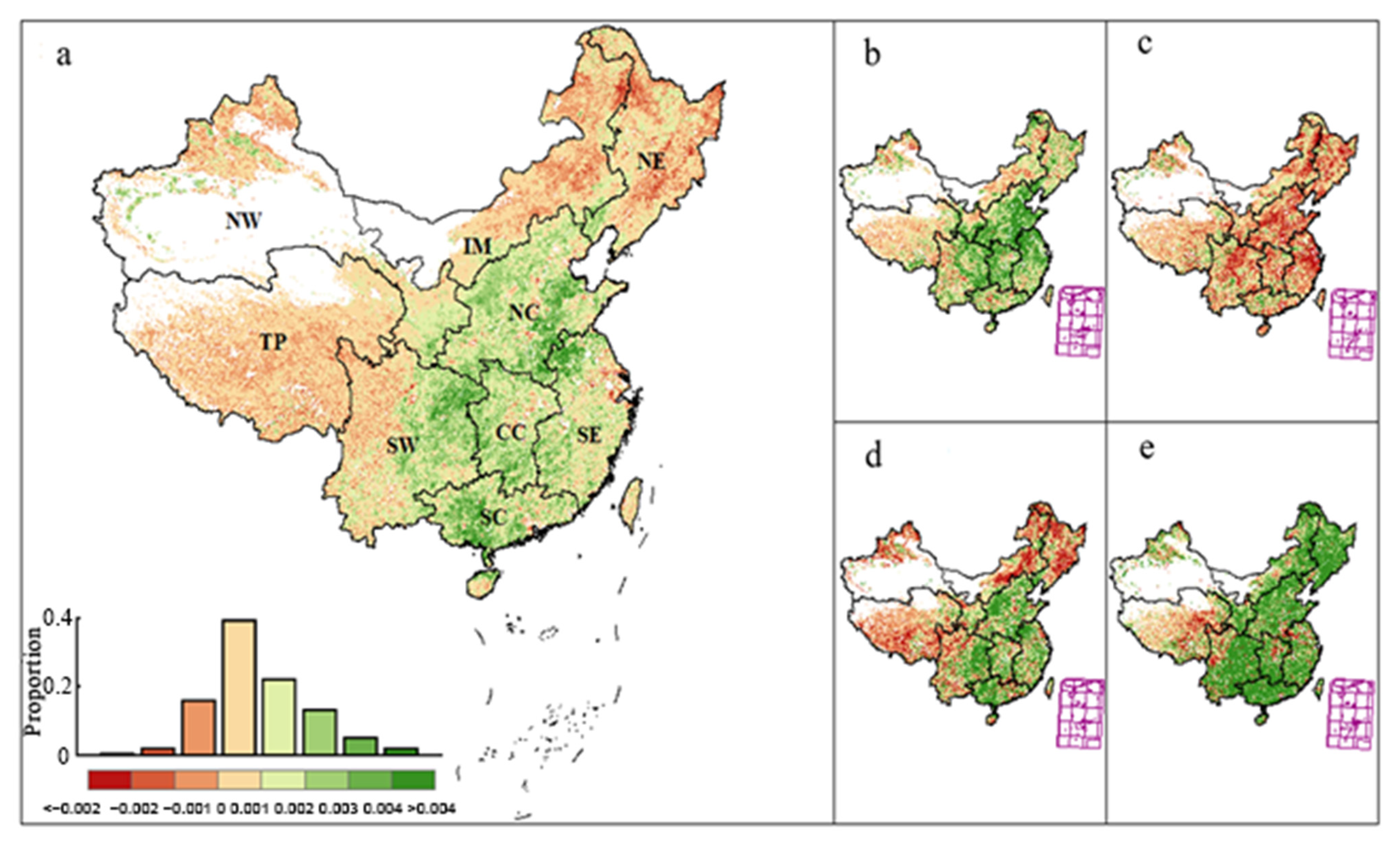
3.2.1. Spatial Changes

According to results from the analysis of the new dataset, the terrestrial ecosystems in China had a mean FPAR of 0.37 during the period of 1980 to 2018 (Figure 1a). Higher FPAR measures, from 0.39 to 0.59, were found over forest areas. South China (SC) had the highest FPAR (0.59) followed by Southeast China (SE), Central China (CC), Southwest China (SW), and Northeast China (NE) with regional means of 0.57, 0.52, 0.50, and 0.39, respectively. Lower FPAR measures were found over grasslands and desert areas with lower values from 0.20 in Northwest China (NW) and the Tibetan Plateau (TP) to 0.25 in Inner Mongolia (IM) and 0.36 in North China (NC). Meanwhile, evergreen broadleaf forests (EBF) had the highest FPAR (0.60) followed by other forests, croplands, shrubland and grasslands (Figure 1c).

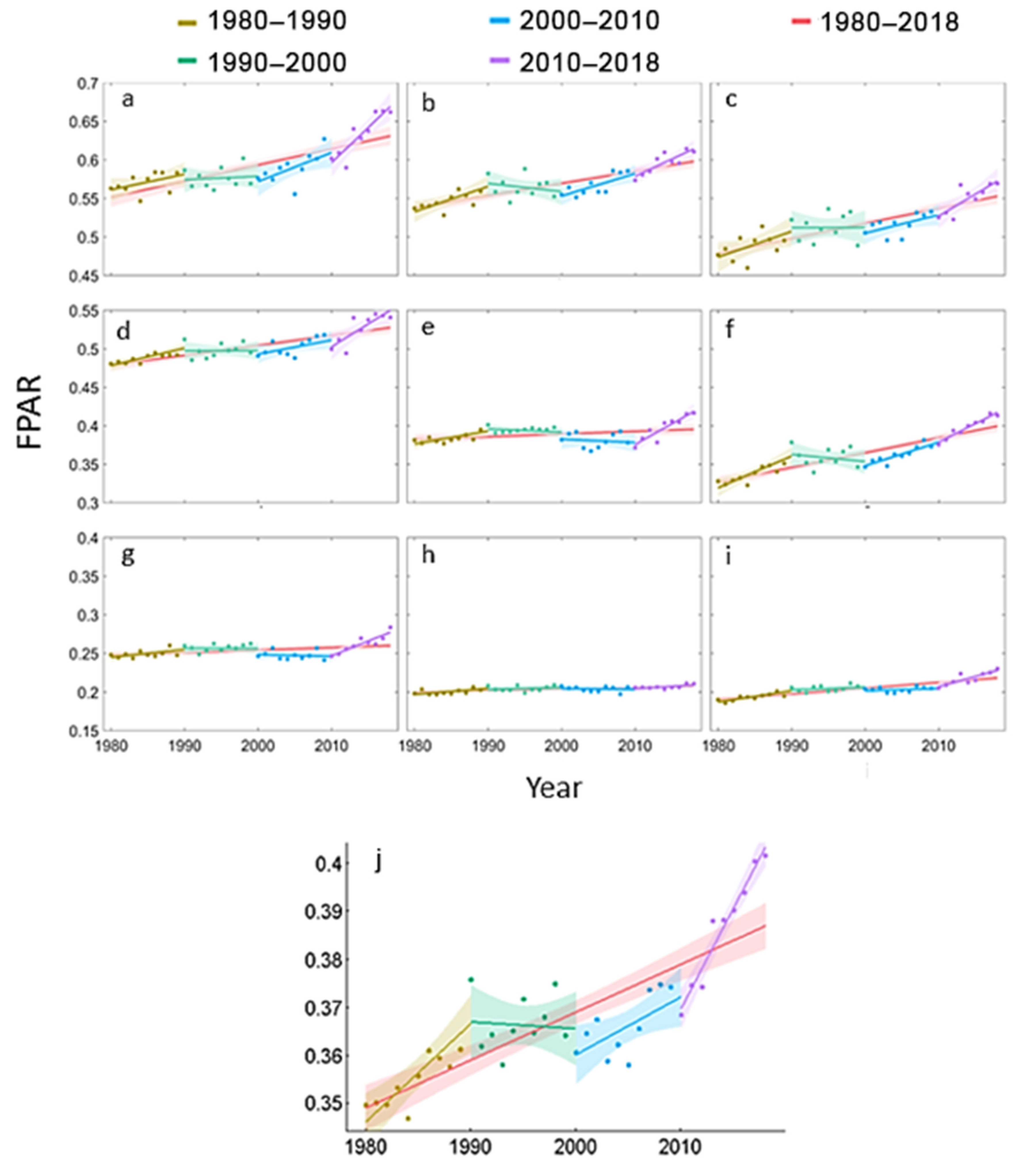
3.2.2. Temporal Trends

The FPAR showed a significant increasing trend with a slope of 0.10% (R² = 0.7, p < 0.01) over Chinese terrestrial ecosystems from 1980 to 2018 (Figure 2). The FPAR was 0.37 during the period from 1980 to 2018, but a turning point emerged around 2010. The regional mean FPAR increased from 0.36 in the first period (1980 to 2010) to 0.39 in the second period (2010 to 2018) and showed an increase of 7 times in the second period with a rate of 0.42% a⁻¹ (R² = 0.95, p < 0.01) compared to the rate of 0.06% a⁻¹ (R² = 0.47, p < 0.01) in the first period (Figure 2, Table S5).

A high increase mainly occurred in southeast and central China while the slowest increase was in the Tibetan Plateau (Figure 3). FPAR increased rapidly in South China (0.21% a⁻¹), Central China (0.20% a⁻¹), North China (0.19% a⁻¹), and Southeast China (0.16% a⁻¹). The growing rates of FPAR were lower in the Tibetan Plateau (0.02% a⁻¹), Inner Mongolia (0.03% a⁻¹), and Northeast China (0.03% a⁻¹). In Northwest China and Southwest China, the growth rates are 0.07% a⁻¹ and 0.13% a⁻¹ (Table S5). The increasing trend of FPAR was significant in the area for 66.9% of the study area with a confidence level above 95% (p < 0.05), and 57% of the area had a confidence level above 99% (p < 0.01). An increasing rate of change was observed mainly in croplands (0.15% a⁻¹) and EBF (0.14% a⁻¹).

The trends for FPAR varied across the four decades over the terrestrial ecosystems in China from 1980 to 2018 (Figure 3). The FPAR showed a rapid and significant increasing trend (p < 0.01) with a rate of 0.20% a⁻¹ over the extended area of 84.5% of the terrestrial ecosystem in China for the decade beginning in 1980. In the 1990s, however, FPAR showed an insignificant decline trend (p = 0.81), with a slope of −0.014% a⁻¹ over all of China, and the total area with an increasing trend accounted for only 49.5% of all vegetated lands. However, a significant upward trend was found again with a slope of 0.12% a⁻¹ (p < 0.05) over 62.1% of the area in the 2000s and further sped up to the rate of 0.42% a⁻¹ with wider spatial scope (83.7%) through the 2010s (Figure S5).

As shown in Figure 4, the stability of FPAR in SC and SW showed a similar trend, i.e., higher in the first two decades and lower in the second two decades. In CC, NW and the whole of China, the stability in the 1990s and 2000s were higher while in the 1980s and 2010s was lower. In SE and NC, there was little difference in stability in each period. The stability of FPAR in NE in the 1990s was higher than in other decades, and it was lower in the last two decades than in the first two decades. In IM, the stability was higher in the first three decades than in the last. In TP, the stability of FPAR gradually improved, and stability in the 2010s was significantly higher than that in the other three periods (Figure 4). We further counted the proportion of areas with high stability in each period, which were 75.89%, 78.05%, 77.72% and 83.33%, respectively, showing that the area with higher variation degree increased after 1990.

3.3. Impacts from Climate Change and Nitrogen Deposition

3.3.1. Climate Change

The impacts from climate change were analyzed by applying random forest regressions with the annual mean air temperature (TAVG), annual total precipitation (ATP), annual total solar shortwave radiation (SWRad), and atmospheric CO₂ concentration as independent variables. Those variables can explain about 55% of the interannual variability in FPAR across the whole country (R² = 0.55 ± 0.19). Regionally, those variables could explain 39% to 51% of the changes in FPAR according to the R² in NC (0.51 ± 0.17), CC (0.48 ± 0.17), SE (0.39 ± 0.18), and NW (0.39 ± 0.16), respectively. A weak influence of climate factors was exerted on the trend of FPAR, as shown by the lower R², in SC (0.32 ± 0.16), IM (0.25 ± 0.18), TP (0.23 ± 0.16), SW (0.18 ± 0.15), and NE (0.13 ± 0.14), respectively.

The interannual variability across China was best explained by TAVG, followed by CO₂ concentration. Such a combination can be found in SC, SE, CC, SW, TP, and NW. SWRad and ATP seemed to be unimportant, except in easterly and northerly areas. Although TAVG was the most important climatic predictor as SWRad was of secondary importance to the trend of FPAR in NE and NC; ATP was of secondary importance in IM (Figure 5 and Figure 6).

3.3.2. Nitrogen Deposition

Linear regression was applied to analyze the effect of nitrogen deposition on the interannual variability in FPAR between 1980 and 2010 (

Table 4. The effect of the nitrogen deposition was analyzed by linear regression for the FPAR over Chinese terrestrial ecosystems from 1980 to 2010.

	Slope	Intercept	${\mathit{R}}^2$	p-Value
SC	0.001	0.557	0.44	<0.001
SE	0.0008	0.539	0.43	<0.001
CC	0.001	0.478	0.43	<0.001
SW	0.0009	0.481	0.47	<0.001
NE	−0.0002	0.389	0.024	>0.05
NC	0.0011	0.328	0.58	<0.001
IM	−0.0003	0.252	0.02	>0.05
TP	0.004	0.201	0.1	>0.05
NW	0.0025	0.193	0.41	<0.001
Total	0.001	0.351	0.46	<0.001

). The results show that nitrogen deposition prompted the growth of FPAR, with the effects of 0.1% g N m⁻² a⁻¹ indicated by the regression coefficient and could explain 46% of the interannual variability in FPAR (R² = 0.46, p < 0.001) across the whole country. The R² varied from 0.02 (p > 0.05) in NE and IM to 0.58 (p < 0.001) in NC. The N deposition had a positive effect in the southeast (0.08% g N m⁻² a⁻¹) and the North China Plain (0.11% g N m⁻² a⁻¹). Significant positive effects were also found in NW, SW, CC, NC, SE and SC, with regression coefficients of 0.0025, 0.0009, 0.001, 0.0011, 0.0008 and 0.001, respectively (p < 0.001). However, the correlation was not significant (p > 0.05) in TP, IM and NE, which would indicate that N deposition may have less effect on FPAR at high latitudes and elevations.

4. Discussion

4.1. FPAR Estimation and Its Uncertainties

In this study, an ANN model-based FPAR_ANN was generated having both longer-term and finer spatial resolution than previously available. Importantly, it was more consistent in terms of spatiotemporal similarity with the FPAR product (MCD15A2) of MODIS. Meanwhile, the NDVI3g and FPAR_BNU showed lower similarity though both data have long-term records [28,56]. The MCD15A2 product was found to have higher performance for present temporal-spatial changes modeling for global vegetation [57,58]. This study, on the other hand, extended the MODIS product back to a final data span from 1980 to 2018 and could be further extended, along with the output of MODIS data, without extra data processing except the SG filter used to remove some noise.

The newly developed FPAR data showed not only more similarity but also comparable performance with the NDVI3g and FPAR_BNU when evaluating with on-the-ground GPP observations from eddy covariance towers in terms of seasonal change. However, it is important to note that satellite remote sensing has inherent uncertainties that can lead to errors in the data. The algorithm of the MODIS product (MCD15A2) itself was found to have uncertainties dependent on its inherent model, input parameters, the effect of vegetation clumping and scale [59,60]. On the other hand, data quality was influenced by some noise induced by clouds, rainy weather and the saturation phenomenon in tropical and subtropical regions [61,62,63], which exerts a great challenge to improving data quality for optical-based remote sensing. Similarly, the new FPAR dataset was influenced by the above factors on quality, which would result in lower performance in sub-tropic or tropic forests. The uncertainty associated with the data will have implications for its application, such as modeling gross primary production. As a result, further research is warranted to enhance the algorithm and improve data quality in future studies [64]. However, the FPAR_ANN data showed comparable performance with more similarity to FPAR_MCD15A2, which makes it useful with its longer period, spanning nearly 4 decades from 1980 to 2018. The data could be potentially applied as inputs for ecosystem modeling, or for soil erosion estimations, and other research on the responses, adaptation and sustainability of terrestrial ecosystems to global changes, benefitting particularly from such a long-term dataset. More importantly, it provides a chance to directly use the upcoming FPAR_MCD15A2 and a method framework to fuse other remote sensing products in future research.

4.2. Spatiotemporal Changes and Underlying Mechanism

A significant increasing trend was found in the FPAR time series for terrestrial ecosystems in China from 1980 to 2018. A similar trend was found in NDVI, which is linearly correlated with FPAR [65,66]. In this study, annual mean air temperature and annual mean carbon dioxide concentrations in the atmosphere were found to have a relatively strong influence on the interannual variability in FPAR over Chinese terrestrial ecosystems.

The turning point around 2010 in the FPAR temporal trend is of great interest, which has been found previously in the trend of vegetation productivity in China, attributed to both natural and human influences [67]. The warming hiatus which occurred around 2012 could be a key factor contributing to this turning point. During this period, global warming continued, but the rate of surface temperature increase slowed down compared to previous decades [68,69]. This hiatus is believed to have been caused by natural variability in the climate system [70]. The climate system’s response to increased greenhouse gases and other human activities was temporarily masked by these natural factors. As the hiatus ended, the warming trend continued, and this may have contributed to the increasing trend in FPAR after 2010. In high latitudes and high elevations (IM, NE, TP), the effect of temperature is greater, and the annual variability of FPAR was also weakly correlated with nitrogen deposition, which may be related to temperature stress under varying precipitation [71]. Climate anomalies have also been found to affect interannual variability in vegetation growth. For example, the anomaly of an Arctic polar vortex was found to have a negative impact on spring vegetation growth in China [72]. Moreover, changes in land use have been found to contribute 30–45% of annual fluctuations in the terrestrial carbon cycle, which means interannual variability of vegetation growth is influenced by human activities. Future research can explore the causes of the turning point around 2010 in more detail and investigate the relative contributions of natural and human influences to regional differences in FPAR trends. Furthermore, it is imperative to undertake a comprehensive analysis of climate sensitivity based on field observations to enhance the accuracy and comprehensiveness of the findings [73].

5. Conclusions

In this study, an artificial neural network (ANN) model, which offers the advantage of effectively handling complex nonlinear relationships, identifying patterns and trends within data, and overcoming limitations associated with inaccurate assumptions or oversimplifications commonly observed in traditional methods, was developed to generate a fraction of absorbed photosynthetically active radiation (FPAR) data. It extends the MODIS product to 1980–2018, from a previous range of 2002–2018, which provides the possibility of direct use of upcoming MODIS products along with our dataset. This new data set was applied to investigate the spatiotemporal dynamics of Chinese terrestrial ecosystems from 1980 to 2018. Results suggest that vegetation growth has increased significantly and has sped up in the most recent decade, with a specific turning point around 2010. The turning point could be attributed to the monsoon climate change indicated by a warming hiatus around 2010. However, though additional research is essential to quantify the contribution from both natural environmental change and human activities, this study provides valuable insights into the spatiotemporal dynamics of FPAR in China and the underlying drivers of these changes. Due to some uncertainties still existing in the new FPAR data, some additional methods could be developed to improve data quality. However, this study not only provides a long-term dataset with lots of potential applications, but also provides a methodological framework for quality improvement of other data in the future, which can be used in further exploration of vegetation dynamic change and carbon stock estimation with longer time series and finer spatial resolution.

References

1. Pan, N.; Feng, X.; Fu, B.; Wang, S.; Ji, F.; Pan, S. Increasing global vegetation browning hidden in overall vegetation greening: Insights from time-varying trends. Remote Sens. Environ. 2018, 214, 59–72. [Google Scholar] [CrossRef]
2. Zhu, Z.; Piao, S.; Myneni, R.B.; Huang, M.; Zeng, Z.; Canadell, J.G.; Ciais, P.; Sitch, S.; Friedlingstein, P.; Arneth, A.; et al. Greening of the Earth and its drivers. Nat. Clim. Chang. 2016, 6, 791–795. [Google Scholar] [CrossRef]
3. He, H.; Wang, S.; Zhang, L.; Wang, J.; Ren, X.; Zhou, L.; Piao, S.; Yan, H.; Ju, W.; Gu, F.; et al. Altered trends in carbon uptake in China’s terrestrial ecosystems under the enhanced summer monsoon and warming hiatus. Natl. Sci. Rev. 2019, 6, 505–514. [Google Scholar] [CrossRef] [PubMed]
4. Wang, Y.; Yan, G.; Hu, R.; Xie, D.; Chen, W. A Scaling-Based Method for the Rapid Retrieval of FPAR From Fine-Resolution Satellite Data in the Remote-Sensing Trend-Surface Framework. IEEE Trans. Geosci. Remote Sens. 2020, 58, 7035–7048. [Google Scholar] [CrossRef]
5. Zhang, Z.; Zhang, Y.; Zhang, Y.; Gobron, N.; Frankenberg, C.; Wang, S.; Li, Z. The potential of satellite FPAR product for GPP estimation: An indirect evaluation using solar-induced chlorophyll fluorescence. Remote Sens. Environ. 2020, 240, 111686. [Google Scholar] [CrossRef]
6. Liang, S.; Wang, J. (Eds.) Chapter 11—Fraction of absorbed photosynthetically active radiation. In Advanced Remote Sensing, 2nd ed.; Academic Press: Cambridge, MA, USA, 2020; pp. 447–476. [Google Scholar]
7. Feng, X.; Liu, G.; Chen, J.M.; Chen, M.; Liu, J.; Ju, W.M.; Sun, R.; Zhou, W. Net primary productivity of China’s terrestrial ecosystems from a process model driven by remote sensing. J. Environ. Manag. 2007, 85, 563–573. [Google Scholar] [CrossRef] [PubMed]
8. Gower, S.T.; Kucharik, C.J.; Norman, J.M. Direct and Indirect Estimation of Leaf Area Index, fAPAR, and Net Primary Production of Terrestrial Ecosystems. Remote Sens. Environ. 1999, 70, 29–51. [Google Scholar] [CrossRef]
9. Myneni, R.; Knyazikhin, Y.; Park, T. MOD15A2H MODIS/Terra Leaf Area Index/FPAR 8-Day L4 Global 500m SIN Grid V006. NASA EOSDIS Land Processes Distributed Active Archive Center. 2015. Available online: https://lpdaac.usgs.gov/products/mod15a2hv006/ (accessed on 10 January 2021).
10. D’Odorico, P.; Gonsamo, A.; Pinty, B.; Gobron, N.; Coops, N.; Mendez, E.; Schaepman, M.E. Intercomparison of fraction of absorbed photosynthetically active radiation products derived from satellite data over Europe. Remote Sens. Environ. 2014, 142, 141–154. [Google Scholar] [CrossRef]
11. Yan, K.; Park, T.; Yan, G.; Chen, C.; Yang, B.; Liu, Z.; Nemani, R.R.; Knyazikhin, Y.; Myneni, R.B. Evaluation of MODIS LAI/FPAR Product Collection 6. Part 1: Consistency and Improvements. Remote Sens. 2016, 8, 359. [Google Scholar] [CrossRef] [Green Version]
12. Pinzon, J.E.; Tucker, C.J. A Non-Stationary 1981–2012 AVHRR NDVI3g Time Series. Remote Sens. 2014, 6, 6929–6960. [Google Scholar] [CrossRef] [Green Version]
13. Kern, A.; Marjanović, H.; Barcza, Z. Evaluation of the Quality of NDVI3g Dataset against Collection 6 MODIS NDVI in Central Europe between 2000 and 2013. Remote Sens. 2016, 8, 955. [Google Scholar] [CrossRef] [Green Version]
14. Fensholt, R.; Proud, S.R. Evaluation of Earth Observation based global long term vegetation trends—Comparing GIMMS and MODIS global NDVI time series. Remote Sens. Environ. 2012, 119, 131–147. [Google Scholar] [CrossRef]
15. Wang, Z.; Wei, C.; Liu, X.; Zhu, L.; Yang, Q.; Wang, Q.; Zhang, Q.; Meng, Y. Object-based change detection for vegetation disturbance and recovery using Landsat time series. GISci. Remote Sens. 2022, 59, 1706–1721. [Google Scholar] [CrossRef]
16. Chu, H.; Venevsky, S.; Wu, C.; Wang, M. NDVI-based vegetation dynamics and its response to climate changes at Amur-Heilongjiang River Basin from 1982 to 2015. Sci. Total Environ. 2019, 650, 2051–2062. [Google Scholar] [CrossRef] [PubMed]
17. Wang, J.; Ding, Y.; Wang, S.; Watson, A.E.; He, H.; Ye, H.; Ouyang, X.; Li, Y. Pixel-scale historical-baseline-based ecological quality: Measuring impacts from climate change and human activities from 2000 to 2018 in China. J. Environ. Manag. 2022, 313, 114944. [Google Scholar] [CrossRef]
18. Feng, G.; Masek, J.; Schwaller, M.; Hall, F. On the blending of the Landsat and MODIS surface reflectance: Predicting daily Landsat surface reflectance. IEEE Trans. Geosci. Remote Sens. 2006, 44, 2207–2218. [Google Scholar] [CrossRef]
19. Zurita-Milla, R.; Clevers, J.G.P.W.; Schaepman, M.E. Unmixing-Based Landsat TM and MERIS FR Data Fusion. IEEE Geosci. Remote Sens. Lett. 2008, 5, 453–457. [Google Scholar] [CrossRef] [Green Version]
20. Kattenborn, T.; Leitloff, J.; Schiefer, F.; Hinz, S. Review on Convolutional Neural Networks (CNN) in vegetation remote sensing. ISPRS J. Photogramm. Remote Sens. 2021, 173, 24–49. [Google Scholar] [CrossRef]
21. Jensen, R.R.; Hardin, P.J.; Yu, G. Artificial Neural Networks and Remote Sensing. Geogr. Compass 2009, 3, 630–646. [Google Scholar] [CrossRef]
22. Yang, T.; Asanjan, A.A.; Welles, E.; Gao, X.; Sorooshian, S.; Liu, X. Developing reservoir monthly inflow forecasts using artificial intelligence and climate phenomenon information. Water Resour. Res. 2017, 53, 2786–2812. [Google Scholar] [CrossRef]
23. Yang, T.; Asanjan, A.A.; Faridzad, M.; Hayatbini, N.; Gao, X.; Sorooshian, S. An enhanced artificial neural network with a shuffled complex evolutionary global optimization with principal component analysis. Inf. Sci. 2017, 418–419, 302–316. [Google Scholar] [CrossRef] [Green Version]
24. Liu, X.; Zhu, X.; Zhang, Q.; Yang, T.; Pan, Y.; Sun, P. A remote sensing and artificial neural network-based integrated agricultural drought index: Index development and applications. Catena 2020, 186, 104394. [Google Scholar] [CrossRef]
25. Jevšenak, J.; Levanič, T. Should artificial neural networks replace linear models in tree ring based climate reconstructions? Dendrochronologia 2016, 40, 102–109. [Google Scholar] [CrossRef]
26. Zhang, L.; Li, X.; Zheng, D.; Zhang, K.; Ma, Q.; Zhao, Y.; Ge, Y. Merging multiple satellite-based precipitation products and gauge observations using a novel double machine learning approach. J. Hydrol. 2021, 594, 125969. [Google Scholar] [CrossRef]
27. Sun, Z.; Wang, J. The 30m-NDVI-Based Alpine Grassland Changes and Climate Impacts in the Three-River Headwaters Region on the Qinghai-Tibet Plateau from 1990 to 2018. J. Resour. Ecol. 2022, 13, 186–195. [Google Scholar] [CrossRef]
28. Zhu, Z.; Bi, J.; Pan, Y.; Ganguly, S.; Anav, A.; Xu, L.; Samanta, A.; Piao, S.; Nemani, R.R.; Myneni, R.B. Global Data Sets of Vegetation Leaf Area Index (LAI)3g and Fraction of Photosynthetically Active Radiation (FPAR)3g Derived from Global Inventory Modeling and Mapping Studies (GIMMS) Normalized Difference Vegetation Index (NDVI3g) for the Period 1981 to 2011. Remote Sens. 2013, 5, 927. [Google Scholar] [CrossRef] [Green Version]
29. Claverie, M.; Matthews, J.L.; Vermote, E.F.; Justice, C.O. A 30+ Year AVHRR LAI and FAPAR Climate Data Record: Algorithm Description and Validation. Remote Sens. 2016, 8, 263. [Google Scholar] [CrossRef] [Green Version]
30. Xiao, Z.; Liang, S.; Sun, R.; Wang, J.; Jiang, B. Estimating the fraction of absorbed photosynthetically active radiation from the MODIS data based GLASS leaf area index product. Remote Sens. Environ. 2015, 171, 105–117. [Google Scholar] [CrossRef]
31. Baret, F.; Weiss, M.; Lacaze, R.; Camacho, F.; Makhmara, H.; Pacholcyzk, P.; Smets, B. GEOV1: LAI and FAPAR essential climate variables and FCOVER global time series capitalizing over existing products. Part1: Principles of development and production. Remote Sens. Environ. 2013, 137, 299–309. [Google Scholar] [CrossRef]
32. Gobron, N.; Pinty, B.; Verstraete, M.; Govaerts, Y. The MERIS Global Vegetation Index (MGVI): Description and preliminary application. Int. J. Remote Sens. 1999, 20, 1917–1927. [Google Scholar] [CrossRef]
33. Gobron, N.; Mélin, F.; Pinty, B.; Verstraete, M.M.; Widlowski, J.L.; Bucini, G. A global vegetation index for SeaWiFS: Design and applications. In Remote Sensing and Climate Modeling: Synergies and Limitations; Beniston, M., Verstraete, M.M., Eds.; Springer: Dordrecht, The Netherlands, 2001; pp. 5–21. [Google Scholar]
34. Baret, F.; Hagolle, O.; Geiger, B.; Bicheron, P.; Miras, B.; Huc, M.; Berthelot, B.; Niño, F.; Weiss, M.; Samain, O.; et al. LAI, fAPAR and fCover CYCLOPES global products derived from VEGETATION: Part 1: Principles of the algorithm. Remote Sens. Environ. 2007, 110, 275–286. [Google Scholar] [CrossRef] [Green Version]
35. Wang, J.; Dong, J.; Yi, Y.; Lu, G.; Oyler, J.; Smith, W.K.; Zhao, M.; Liu, J.; Running, S. Decreasing net primary production due to drought and slight decreases in solar radiation in China from 2000 to 2012. J. Geophys. Res. Biogeosci. 2017, 122, 261–278. [Google Scholar] [CrossRef] [Green Version]
36. Keith, H.; van Gorsel, E.; Jacobsen, K.L.; Cleugh, H. Dynamics of carbon exchange in a Eucalyptus forest in response to interacting disturbance factors. Agric. For. Meteorol. 2012, 153, 67–81. [Google Scholar] [CrossRef]
37. Liu, J.; Kuang, W.; Zhang, Z.; Xu, X.; Qin, Y.; Ning, J.; Zhou, W.; Zhang, S.; Li, R.; Yan, C.; et al. Spatiotemporal characteristics, patterns, and causes of land-use changes in China since the late 1980s. J. Geogr. Sci. 2014, 24, 195–210. [Google Scholar] [CrossRef]
38. Jonsson, P.; Eklundh, L. TIMESAT—A program for analyzing time-series of satellite sensor data. Comput. Geosci. 2004, 30, 833–845. [Google Scholar] [CrossRef] [Green Version]
39. Tucker, C.J.; Pinzon, J.E.; Brown, M.E.; Slayback, D.A.; Pak, E.W.; Mahoney, R.; Vermote, E.F.; El Saleous, N. An extended AVHRR 8-km NDVI dataset compatible with MODIS and SPOT vegetation NDVI data. Int. J. Remote Sens. 2005, 26, 4485–4498. [Google Scholar] [CrossRef]
40. Xiao, Z.; Liang, S.; Sun, R. Evaluation of Three Long Time Series for Global Fraction of Absorbed Photosynthetically Active Radiation (FAPAR) Products. IEEE Trans. Geosci. Remote Sens. 2018, 56, 5509–5524. [Google Scholar] [CrossRef]
41. Yu, G.; Ren, W.; Chen, Z.; Zhang, L.; Wang, Q.; Wen, X.; He, N.; Zhang, L.; Fang, H.; Zhu, X.; et al. Construction and progress of Chinese terrestrial ecosystem carbon, nitrogen and water fluxes coordinated observation. J. Geogr. Sci. 2016, 26, 803–826. [Google Scholar] [CrossRef] [Green Version]
42. Wang, J.; Wang, J.; Ye, H.; Liu, Y.; He, H. An interpolated temperature and precipitation dataset at 1-km grid resolution in China (2000–2012). China Sci. Data 2017, 2. [Google Scholar] [CrossRef]
43. Bonan, G.B. A computer model of the solar radiation, soil moisture, and soil thermal regimes in boreal forests. Ecol. Model. 1989, 45, 275–306. [Google Scholar] [CrossRef]
44. Wang, J.; Ye, H. An interpolated meteorological dataset at every 8 days, 1-km resolution in China. China Sci. Data 2021, 2. [Google Scholar] [CrossRef]
45. Keeling, C.D.; Piper, S.C.; Bacastow, R.B.; Wahlen, M.; Whorf, T.P.; Heimann, M.; Meijer, H.A.J. Exchanges of Atmospheric CO2 and 13CO2 with the Terrestrial Biosphere and Oceans from 1978 to 2000. I. Global Aspects; SIO Reference Series, No. 01-06; UC San Diego, Scripps Institution of Oceanography: La Jolla, CA, USA, 2001; Volume 88. [Google Scholar]
46. Li, Y.; Yang, X.; Wang, M.; Xu, Y. Precipitation, Cloud and Atmospheric CO2 Interannual Variability. J. Univ. Chin. Acad. Sci. 2005, 22, 394–399. [Google Scholar]
47. Zhang, Y.; Jin, J.-L.; Yan, P.; Tang, J.; Fang, S.-X.; Lin, W.-L.; Lou, M.-Y.; Liang, M.; Zhou, Q.; Jing, J.-S.; et al. Long-term variations of major atmospheric compositions observed at the background stations in three key areas of China. Adv. Clim. Chang. Res. 2020, 11, 370–380. [Google Scholar] [CrossRef]
48. Wu, H. Sampling data of Waliguan carbon monoxide concentration bottle in 1990–2016. 2018. Available online: https://cstr.cn/CSTR:11738.11.ncdc.CGAWBO.2020.30 (accessed on 1 May 2021).
49. Gu, F.; Huang, M.; Zhang, Y.; Yan, H.; Li, J.; Guo, R.; Zhong, X. Modeling the temporal-spatial patterns of atmospheric nitrogen deposition in China during 1961–2010. Acta Ecol. Sin. 2016, 36, 3591–3600. [Google Scholar]
50. Lin, B.-L.; Sakoda, A.; Shibasaki, R.; Goto, N.; Suzuki, M. Modelling a global biogeochemical nitrogen cycle in terrestrial ecosystems. Ecol. Model. 2000, 135, 89–110. [Google Scholar] [CrossRef]
51. Goetz, S.J.; Prince, S.D.; Small, J.; Gleason, A.C.R. Interannual variability of global terrestrial primary production: Results of a model driven with satellite observations. J. Geophys. Res. Atmos. 2000, 105, 20077–20091. [Google Scholar] [CrossRef]
52. Knoben, W.J.M.; Freer, J.E.; Woods, R.A. Technical note: Inherent benchmark or not? Comparing Nash–Sutcliffe and Kling–Gupta efficiency scores. Hydrol. Earth Syst. Sci. 2019, 23, 4323–4331. [Google Scholar] [CrossRef] [Green Version]
53. Wang, Z.; Bovik, A.C.; Sheikh, H.R.; Simoncelli, E.P. Image quality assessment: From error visibility to structural similarity. IEEE Trans. Image Process. 2004, 13, 600–612. [Google Scholar] [CrossRef] [Green Version]
54. Tilman, D.; Reich, P.B.; Knops, J.M. Biodiversity and ecosystem stability in a decade-long grassland experiment. Nature 2006, 441, 629–632. [Google Scholar] [CrossRef]
55. Yin, L.; Tao, F.; Chen, Y.; Liu, F.; Hu, J. Improving terrestrial evapotranspiration estimation across China during 2000–2018 with machine learning methods. J. Hydrol. 2021, 600, 126538. [Google Scholar] [CrossRef]
56. Zhao, X.; Liang, S.; Liu, S.; Yuan, W.; Xiao, Z.; Liu, Q.; Cheng, J.; Zhang, X.; Tang, H.; Zhang, X.; et al. The Global Land Surface Satellite (GLASS) Remote Sensing Data Processing System and Products. Remote Sens. 2013, 5, 2436. [Google Scholar] [CrossRef] [Green Version]
57. Liu, L.; Bai, Y.; Sun, R.; Niu, Z. Stereo Observation and Inversion of the Key Parameters of Global Carbon Cycle: Project Overview and Mid-Term Progressess. Remote Sens. Technol. Appl. 2021, 36, 11–24. [Google Scholar]
58. Fang, H.; Zhang, Y.; Wei, S.; Li, W.; Ye, Y.; Sun, T.; Liu, W. Validation of global moderate resolution leaf area index (LAI) products over croplands in northeastern China. Remote Sens. Environ. 2019, 233, 111377. [Google Scholar] [CrossRef]
59. Xu, B.; Park, T.; Yan, K.; Chen, C.; Zeng, Y.; Song, W.; Yin, G.; Li, J.; Liu, Q.; Knyazikhin, Y.; et al. Analysis of global LAI/FPAR products from VIIRS and MODIS sensors for spatio-temporal consistency and uncertainty from 2012–2016. Forests 2018, 9, 73. [Google Scholar] [CrossRef] [Green Version]
60. Pu, J.; Yan, K.; Zhou, G.; Lei, Y.; Zhu, Y.; Guo, D.; Li, H.; Xu, L.; Knyazikhin, Y.; Myneni, R.B. Evaluation of the MODIS LAI/FPAR Algorithm Based on 3D-RTM Simulations: A Case Study of Grassland. Remote Sens. 2020, 12, 3391. [Google Scholar] [CrossRef]
61. Hilker, T.; Lyapustin, A.I.; Tucker, C.J.; Sellers, P.J.; Hall, F.G.; Wang, Y. Remote sensing of tropical ecosystems: Atmospheric correction and cloud masking matter. Remote Sens. Environ. 2012, 127, 370–384. [Google Scholar] [CrossRef] [Green Version]
62. Liu, S.; Wei, X.; Li, D.; Lu, D. Examining Forest Disturbance and Recovery in the Subtropical Forest Region of Zhejiang Province Using Landsat Time-Series Data. Remote Sens. 2017, 9, 479. [Google Scholar] [CrossRef] [Green Version]
63. Li, Y.; Li, M.; Li, C.; Liu, Z. Forest aboveground biomass estimation using Landsat 8 and Sentinel-1A data with machine learning algorithms. Sci. Rep. 2020, 10, 9952. [Google Scholar] [CrossRef]
64. Shahzaman, M.; Zhu, W.; Ullah, I.; Mustafa, F.; Bilal, M.; Ishfaq, S.; Nisar, S.; Arshad, M.; Iqbal, R.; Aslam, R.W. Comparison of Multi-Year Reanalysis, Models, and Satellite Remote Sensing Products for Agricultural Drought Monitoring over South Asian Countries. Remote Sens. 2021, 13, 3294. [Google Scholar] [CrossRef]
65. Myneni, R.B.; Williams, D.L. On the Relationship between Fapar and Ndvi. Remote Sens. Environ. 1994, 49, 200–211. [Google Scholar] [CrossRef]
66. Zong, J.; Bai, S.; Feng, C.; Pu, Y. Spatiotemporal Variation Characteristics of Ecological Status in China Based on Continuous Time Series NDVI Data. Res. Soil Water Conserv. 2021, 28, 132–138. [Google Scholar]
67. Chen, Y.; Feng, X.; Tian, H.; Wu, X.; Gao, Z.; Feng, Y.; Piao, S.; Lv, N.; Pan, N.; Fu, B. Accelerated increase in vegetation carbon sequestration in China after 2010: A turning point resulting from climate and human interaction. Glob. Chang. Biol. 2021, 27, 5848–5864. [Google Scholar] [CrossRef] [PubMed]
68. Fyfe, J.C.; Meehl, G.A.; England, M.H.; Mann, M.E.; Santer, B.D.; Flato, G.M.; Hawkins, E.; Gillett, N.P.; Xie, S.-P.; Kosaka, Y.; et al. Making sense of the early-2000s warming slowdown. Nat. Clim. Chang. 2016, 6, 224–228. [Google Scholar] [CrossRef] [Green Version]
69. Stocker, T. Climate Change 2013: The Physical Science Basis: Working Group I Contribution to the Fifth Assessment Report of the Intergovernmental Panel on Climate Change; Cambridge University Press: Cambridge, UK, 2014. [Google Scholar]
70. Kosaka, Y.; Xie, S.-P. Recent global-warming hiatus tied to equatorial Pacific surface cooling. Nature 2013, 501, 403–407. [Google Scholar] [CrossRef] [Green Version]
71. Zhao, J.; Luo, T.; Li, R.; Wei, H.; Li, X.; Du, M.; Tang, Y. Precipitation alters temperature effects on ecosystem respiration in Tibetan alpine meadows. Agric. For. Meteorol. 2018, 252, 121–129. [Google Scholar] [CrossRef]
72. Gong, H.; Huang, M.; Wang, Z.; Wang, S.; Gu, F. Anomalous arctic polar vortex-induced spring vegetation variability and lagged productivity responses in China. Theor. Appl. Climatol. 2021, 145, 261–272. [Google Scholar] [CrossRef]
73. Yang, Y.; Roderick, M.L.; Zhang, S.; McVicar, T.R.; Donohue, R.J. Hydrologic implications of vegetation response to elevated CO2 in climate projections. Nature Clim. Chang. 2019, 9, 44–48. [Google Scholar] [CrossRef]
Figure 1. The ANN-based FPAR developed in this study (FPARANN) over Chinese terrestrial ecosystems from 1980 to 2018 and its validations and evaluations. (a) the mean FPAR from 1980 to 2018 and the sites map for the flux towers. (b) The FPARANN was validated through the observed GPP on the eight flux towers of ChinaFLUX and the results were shown by the coefficient of determination (R2). (c) the mean FPAR of each vegetation classification was compared among the FPARANN, the product of the MODIS (FPARMCD15A2) and the GLASS (FPARBNU). These eight flux towers are Yucheng cropland (YC), Dangxiong alpine steppe-meadow (DX), Haibei alpine shrub-meadow (HBGC), Inner Mongolia temperate steppe (NMG), Dinghushan evergreen mixed forest (DHS), Changbaishan temperate mixed forest (CBS), Qianyanzhou evergreen needleleaf forest (QYZ), Xishuangbanna evergreen broadleaf forest (XSBN).
Remotesensing 15 03707 g001
Figure 2. The inter-annual variability and the linear trend of the ANN-based FPAR (FPARANN) developed in this study over the terrestrial ecosystems in China and its nine regions for the whole period from 1980 to 2018 and for each decade. (a) South China (SC), (b) Southeast China (SE), (c) Central China (CC), (d) Southwest China (SW), (e) Northeast China (NE), (f) North China (NC), (g) Inner Mongolia (IM), (h) Tibetan Plateau (TP), (i) Northwest China (NW), and (j) the whole China.
Remotesensing 15 03707 g002
Figure 3. The pixel-scale trend of the FPAR over Chinese terrestrial ecosystems for the whole period from 1980 to 2018 (a) and for the four decades 1980s (b), 1990s (c), 2000s (d) and 2010s (e). The subset in (a) is the area proportion of the slope of the FPAR during 1980–2018 to the total vegetated area.
Remotesensing 15 03707 g003
Figure 4. The temporal stability of the FPAR of the terrestrial ecosystems in China and its nine regions in each decade from 1980 to 2018.
Remotesensing 15 03707 g004
Figure 5. The importance of the climate variables, annual average air temperature (TAVG), annual total precipitation (ATP), annual total solar shortwave radiation (SWRad) and atmospheric CO2 concentration on the interannual variability of the FPAR of the terrestrial ecosystems in China and its nine regions from 1980 to 2018. The importance was quantified by the OOB error rate in random forest regression.
Remotesensing 15 03707 g005
Figure 6. The relationship between FPAR and each climate variable over the terrestrial ecosystems in China and its nine regions from 1980 to 2018. The independent variables include annual average air temperature (TAVG), annual total precipitation (ATP), annual total solar shortwave radiation (SWRad) and atmosphere CO2 concentration. The FPAR and the climate variables were normalized by the z-score method.
Remotesensing 15 03707 g006