

Using Robust Regression to Retrieve Soil Moisture from CyGNSS Data
 , , ,
, , ,
Abstract
:1. Introduction
2. Datasets
2.1. CyGNSS Data
2.2. SMAP Data
2.3. In Situ Data
3. Methods
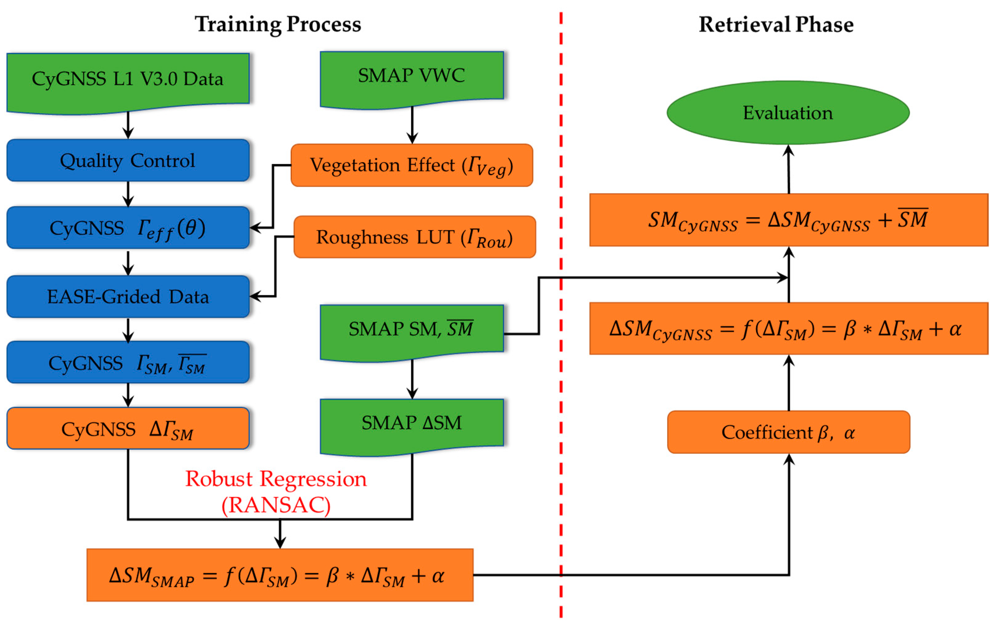
3.1. SM Retrieval Method
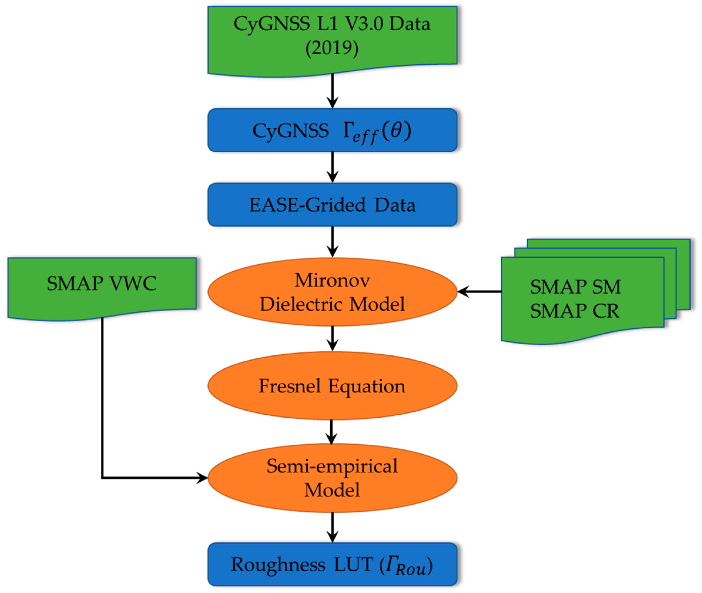
3.2. Estimation of Roughness
3.3. Validation Metrics
4. Results
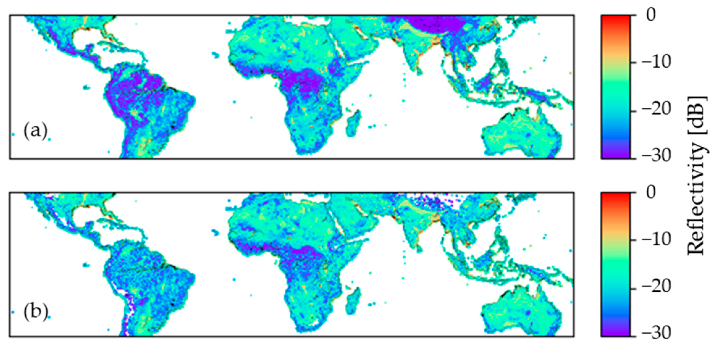
4.1. Calibration of Reflectivity
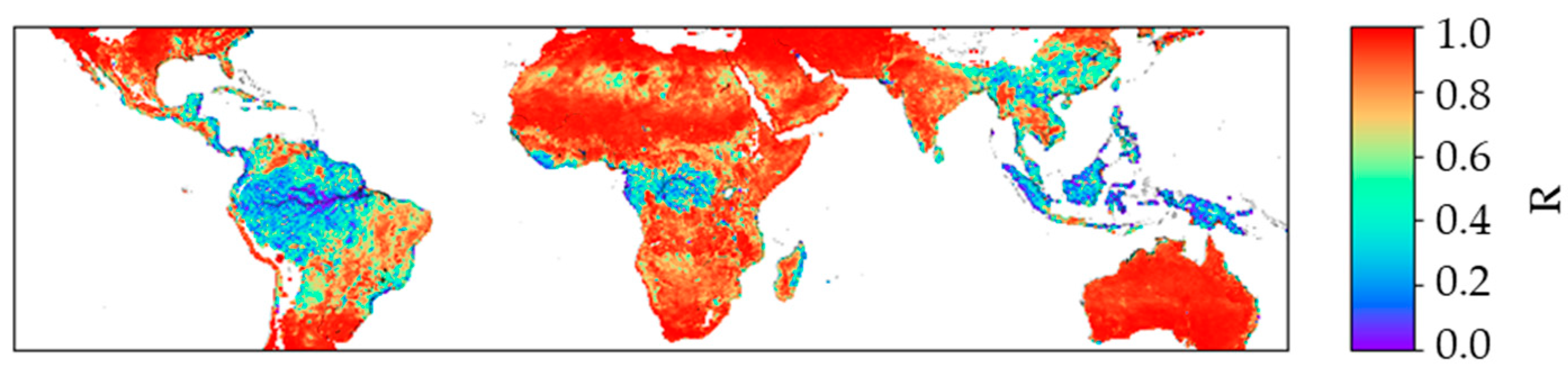
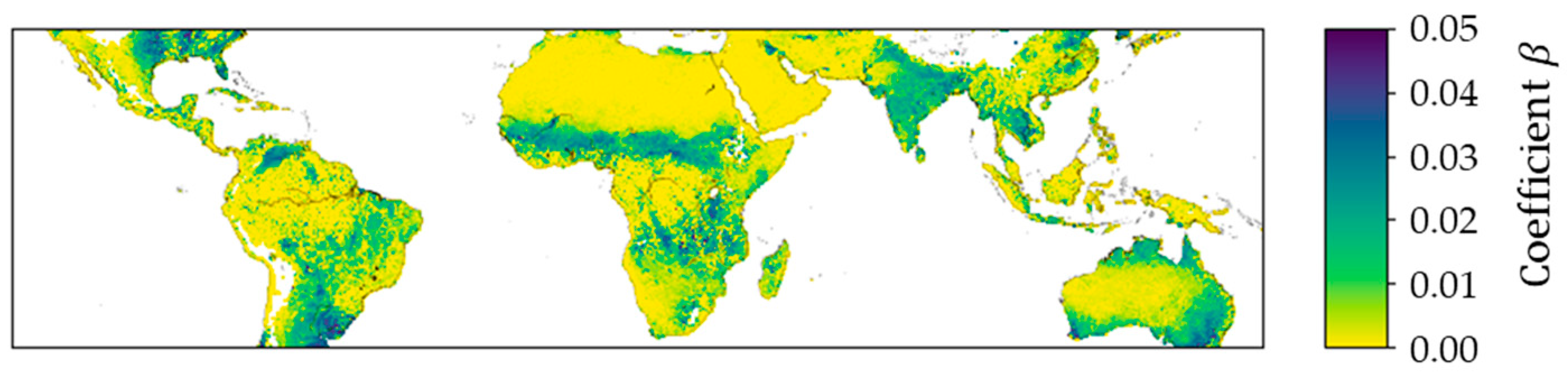
4.2. Estimation of Coefficients
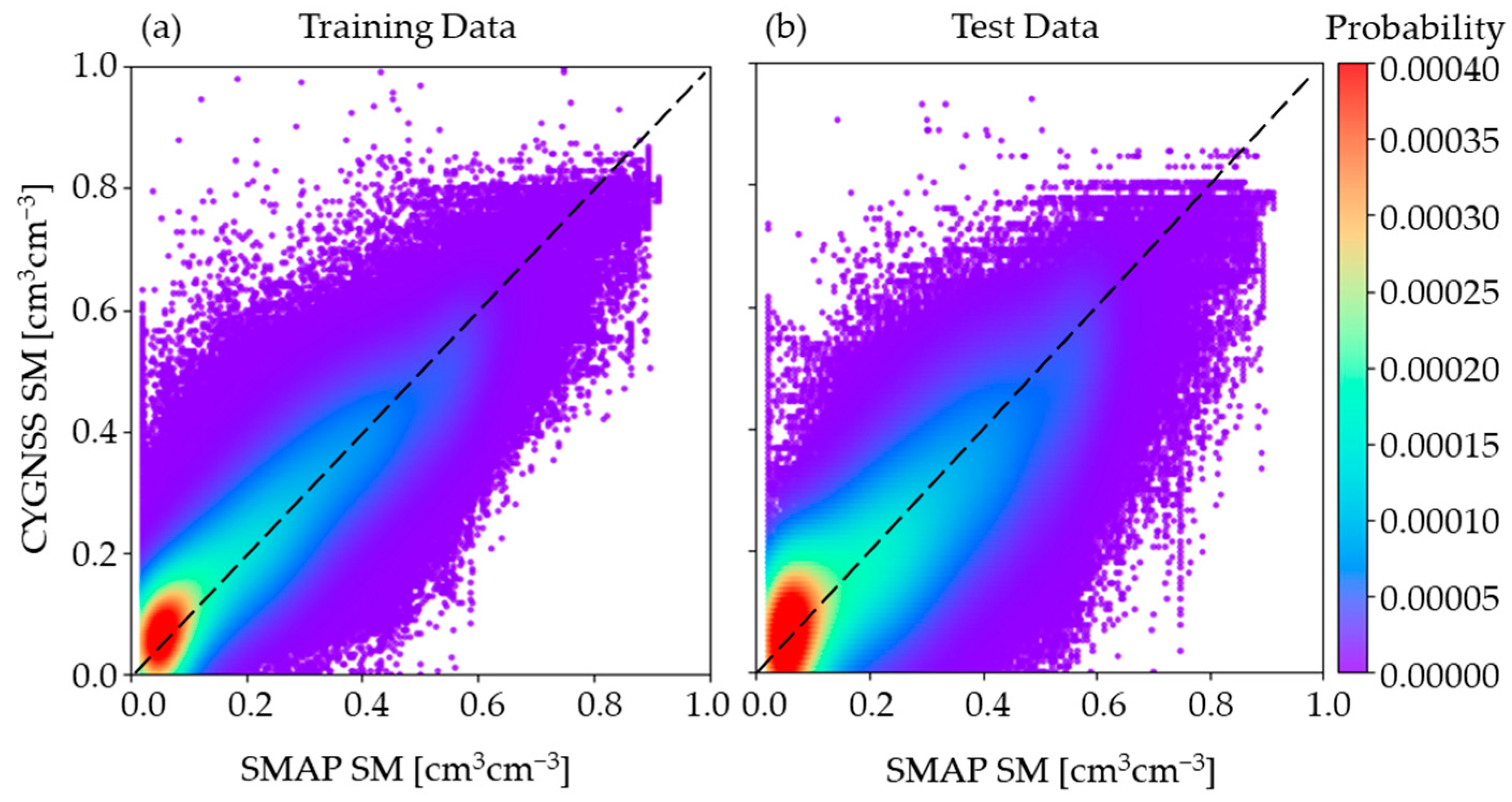
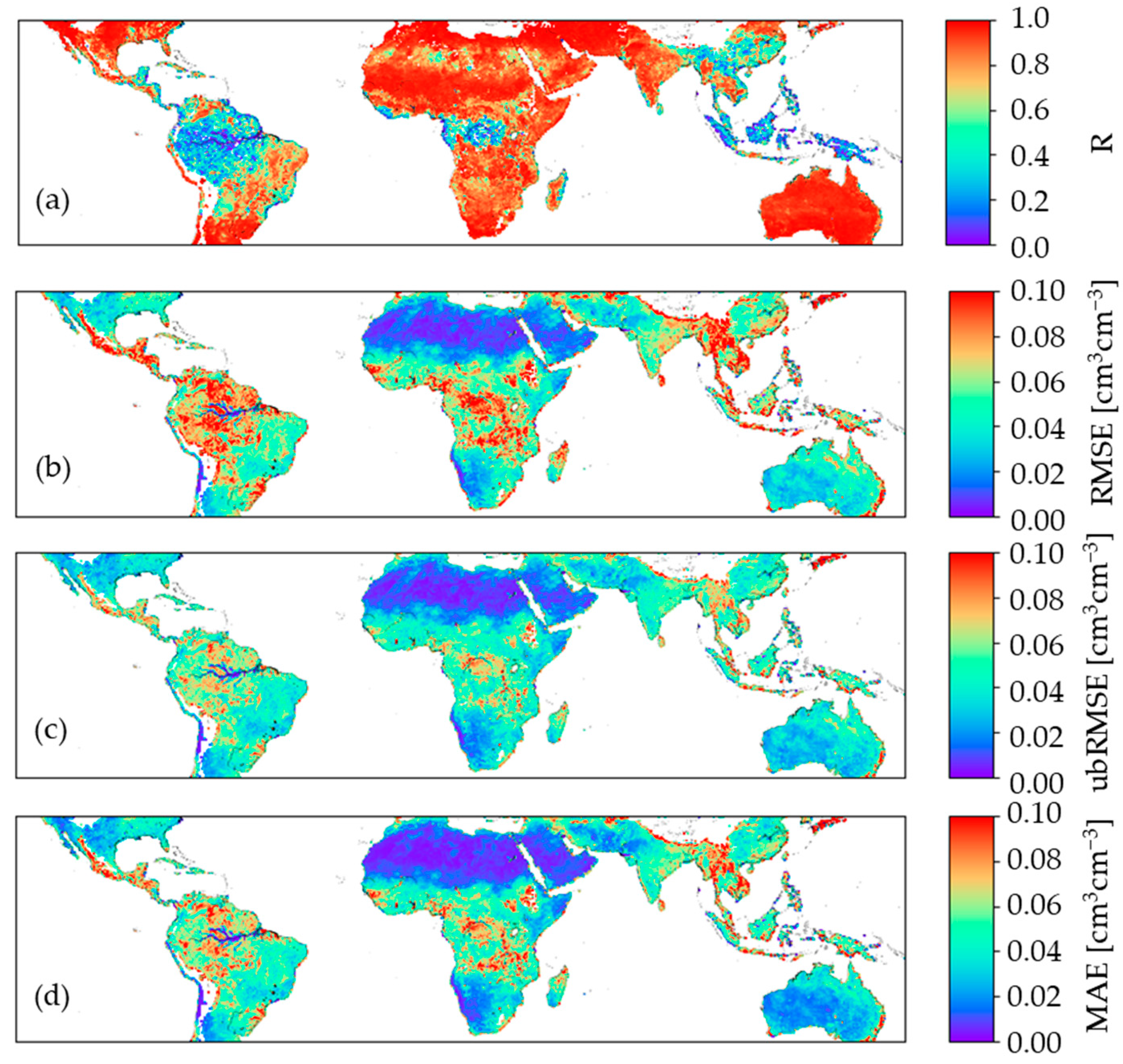
4.3. Evaluation of the Retrieved SM
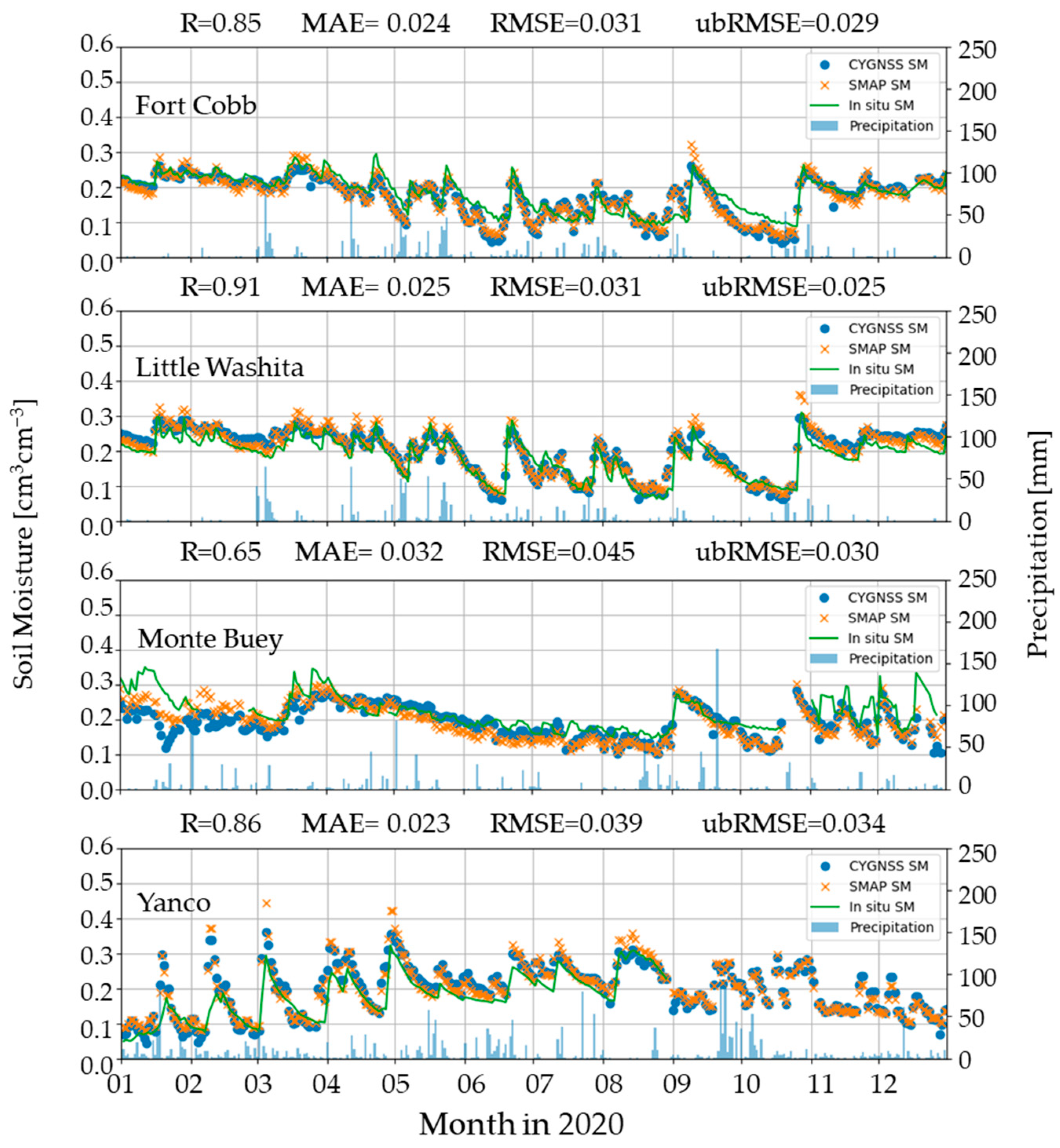
4.4. Validation Using the In Situ Measurements
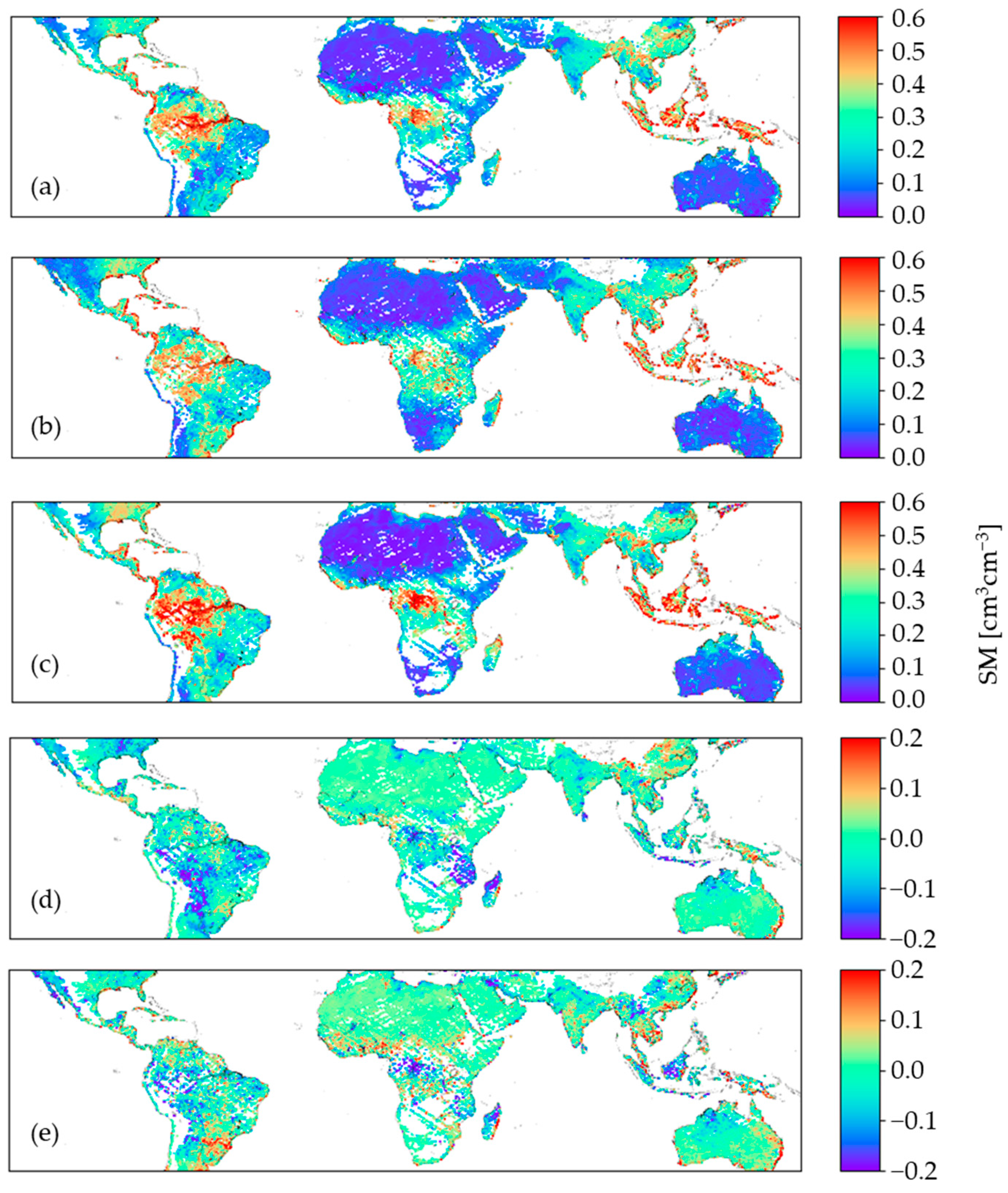
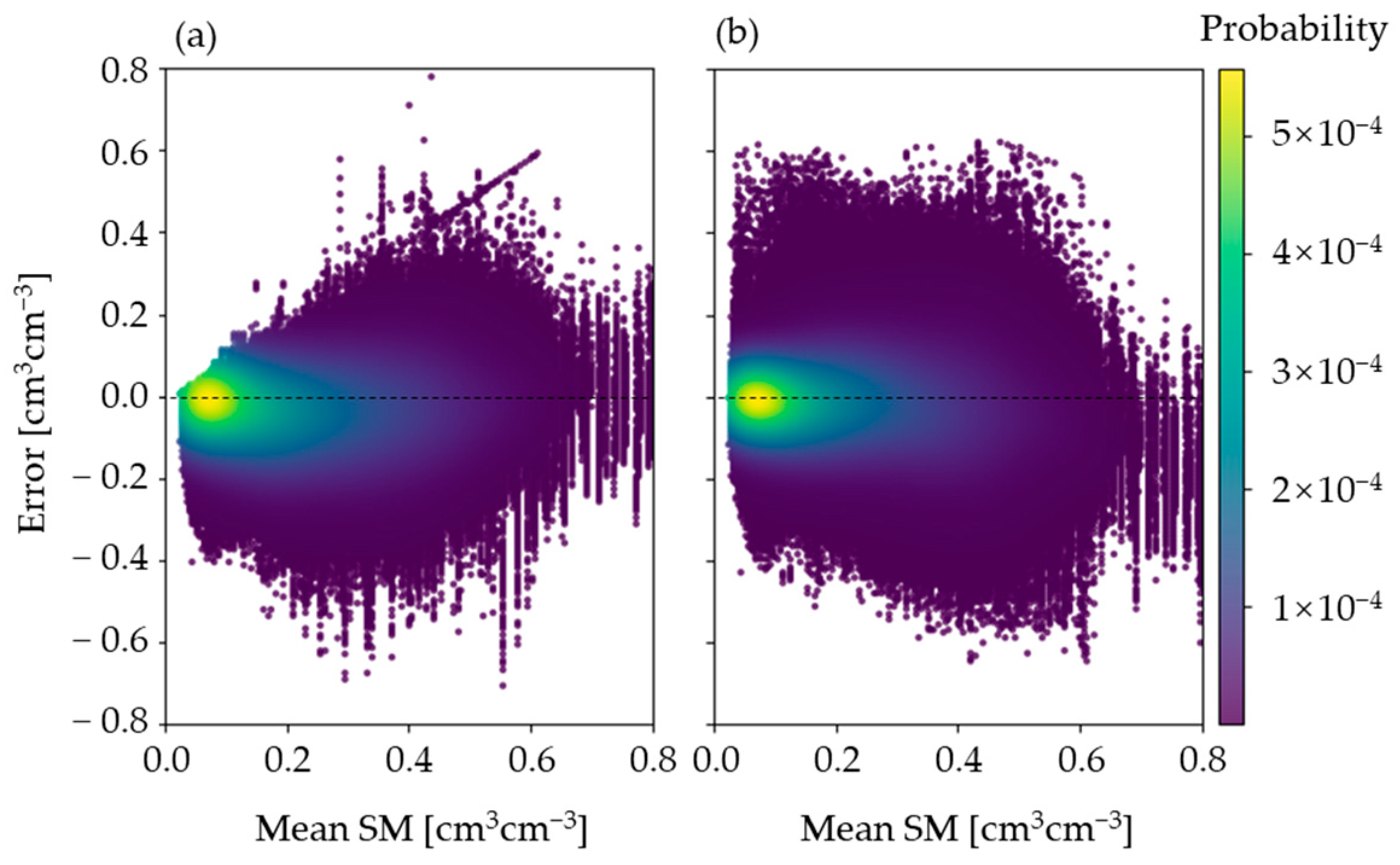
4.5. Comparison of UCAR SM Products
5. Discussions
6. Conclusions
Author Contributions
Funding
Data Availability Statement
Acknowledgments
Conflicts of Interest
References
- Bennett, A.C.; Penman, T.D.; Arndt, S.K.; Roxburgh, S.H.; Bennett, L.T. Climate more important than soils for predicting forest biomass at the continental scale. Ecography 2020, 43, 1692–1705. [Google Scholar] [CrossRef]
- Bojinski, S.; Verstraete, M.; Peterson, T.C.; Richter, C.; Simmons, A.; Zemp, M. The concept of essential climate variables in support of climate research, applications, and policy. Bull. Am. Meteorol. Soc. 2014, 95, 1431–1443. [Google Scholar] [CrossRef] [Green Version]
- Entekhabi, D.; Das, N.; Njoku, E.; Johnson, J.; Shi, J. SMAP L3 Radar/Radiometer Global Daily 9 km EASE-Grid Soil Moisture, Version 3; NASA National Snow and Ice Data Center Distributed Active Archive Center: Boulder, CO, USA, 2016. [Google Scholar] [CrossRef]
- Paul, A.R.; Raj, K. NASA-ISRO SAR (NISAR) Mission Status. In Proceedings of the 2021 IEEE Radar Conference (RadarConf21), Atlanta, GA, USA, 7–14 May 2021; pp. 1–6. [Google Scholar] [CrossRef]
- Ruf, C.S.; Atlas, R.; Chang, P.S.; Clarizia, M.P.; Garrison, J.L.; Gleason, S.; Katzberg, S.J.; Jelenak, Z.; Johnson, J.T.; Majumdar, S.J.; et al. New Ocean Winds Satellite Mission to Probe Hurricanes and Tropical Convection. Bull. Amer. Meteor. Soc. 2016, 97, 385–395. [Google Scholar] [CrossRef]
- Camps, A.; Park, H.; Pablos, M.; Foti, G.; Gommenginger, C.P.; Liu, P.; Judge, J. Sensitivity of GNSS-R Spaceborne Observations to Soil Moisture and Vegetation. IEEE J. Sel. Topics Appl. Earth Observ. Remote Sens. 2016, 9, 4730–4742. [Google Scholar] [CrossRef] [Green Version]
- Chew, C.; Shah, R.; Zuffada, C.; Hajj, G.; Masters, D.; Mannucci, A.J. Demonstrating soil moisture remote sensing with observations from the UK TechDemoSat-1 satellite mission. Geophys. Res. Lett. 2016, 43, 3317–3324. [Google Scholar] [CrossRef] [Green Version]
- Clarizia, M.P.; Pierdicca, N.; Costantini, F.; Floury, N. Analysis of CyGNSS data for soil moisture retrieval. IEEE J. Sel. Topics Appl. Earth Observ. Remote Sens. 2019, 12, 2227–2235. [Google Scholar] [CrossRef]
- Zhang, S.; Ma, Z.; Li, Z.; Zhang, P.; Liu, Q.; Nan, Y.; Zhang, J.; Hu, S.; Feng, Y.; Zhao, H. Using CyGNSS Data to Map Flood Inundation during the 2021 Extreme Precipitation in Henan Province, China. Remote Sens. 2021, 13, 5181. [Google Scholar] [CrossRef]
- Chew, C.; Reager, J.T.; Small, E. CyGNSS data map flood inundation during the 2017 Atlantic hurricane season. Sci. Rep. 2018, 8, 9336. [Google Scholar] [CrossRef]
- Chew, C.; Small, E. Estimating inundation extent using CyGNSS data: A conceptual modeling study. Remote Sens. Environ. 2020, 246, 111869. [Google Scholar] [CrossRef]
- Molina, I.; Calabia, A.; Jin, S.; Edokossi, K.; Wu, X. Calibration and Validation of CyGNSS Reflectivity through Wetlands’ and Deserts’ Dielectric Permittivity. Remote Sens. 2022, 14, 3262. [Google Scholar] [CrossRef]
- Jia, Y.; Savi, P. Sensing soil moisture and vegetation using GNSS-R polarimetric measurement. Adv. Space Res. 2017, 59, 858–869. [Google Scholar] [CrossRef]
- Wu, X.; Guo, P.; Sun, Y.; Liang, H.; Zhang, X.; Bai, W. Recent Progress on Vegetation Remote Sensing Using Spaceborne GNSS-Reflectometry. Remote Sens. 2021, 13, 4244. [Google Scholar] [CrossRef]
- Lei, F.; Senyurek, V.Y.; Kurum, M.; Gurbuz, A.C.; Boyd, D.R.; Moorhead, R.J.; Crow, W.; Eroglu, O. Quasi-global machine learning-based soil moisture estimates at high spatio-temporal scales using CyGNSS and SMAP observations. Remote Sens. Environ. 2022, 276, 113041. [Google Scholar] [CrossRef]
- Senyurek, V.; Lei, F.; Boyd, D.; Kurum, M.; Gurbuz, A.C.; Moorhead, R. Machine Learning-Based CyGNSS Soil Moisture Estimates over ISMN sites in CONUS. Remote Sens. 2020, 12, 1168. [Google Scholar] [CrossRef] [Green Version]
- Eroglu, O.; Kurum, M.; Boyd, D.; Gurbuz, A.C. High Spatio-Temporal Resolution CyGNSS Soil Moisture Estimates Using Artificial Neural Networks. Remote Sens. 2019, 11, 2272. [Google Scholar] [CrossRef] [Green Version]
- Santi, E.; Clarizia, M.P.; Comite, D.; Dente, L.; Guerriero, L.; Pierdicca, N.; Floury, N. Combining CyGNSS and Machine Learning for Soil Moisture and Forest Biomass Retrieval in View of the ESA Scout Hydrognss Mission. In Proceedings of the IEEE International Geoscience and Remote Sensing Symposium, Kuala Lumpur, Malaysia, 17–22 July 2022; pp. 7433–7436. [Google Scholar] [CrossRef]
- Yan, J.; Jin, S.; Chen, H.; Yan, Q.; Patrizia, S.; Jin, Y.; Yuan, Y. Temporal-Spatial Soil Moisture Estimation from CyGNSS Using Machine Learning Regression with a Preclassification Approach. IEEE J. Sel. Top. Appl. Earth Obs. Remote Sens. 2021, 14, 4879–4893. [Google Scholar] [CrossRef]
- Yan, Q.; Huang, W.; Jin, S.; Jia, Y. Pan-tropical soil moisture mapping based on a three-layer model from CyGNSS GNSS-R data. Remote Sens. Environ. 2020, 247, 111944. [Google Scholar] [CrossRef]
- Chew, C.; Small, E. Description of the UCAR/CU Soil Moisture Product. Remote Sens. 2020, 12, 1558. [Google Scholar] [CrossRef]
- Gleason, S.; Ruf, C.S.; O’Brien, A.J.; McKague, D.S. The CYGNSS Level 1 Calibration Algorithm and Error Analysis Based on On-Orbit Measurements. IEEE J. Sel. Top. Appl. Earth Obs. Remote Sens. 2018, 12, 37–49. [Google Scholar] [CrossRef]
- Ren, B.; Zhu, J.; Tsang, L.; Xu, H. Analytical Kirchhoff Solutions (AKS) and Numerical Kirchhoff Approach (NKA) for First-Principle Calculations of Coherent Waves and Incoherent Waves at P Band and L Band in Signals of Opportunity (SoOp). Prog. Electromagn. Res. 2021, 171, 35–73. [Google Scholar] [CrossRef]
- Yueh, S.; Shah, R.; Chaubell, M.J.; Hayashi, A.; Xu, X.; Colliander, A. A semi-empirical modeling of soil moisture, vegetation, and surface roughness impact on CyGNSS reflectometry data. IEEE Trans. Geosci. Remote Sens. 2020, 60, 5800117. [Google Scholar] [CrossRef]
- Al-Khaldi, M.M.; Johnson, J.T.; O’Brien, A.J.; Balenzano, A.; Mattia, F. Time-Series Retrieval of Soil Moisture Using CyGNSS. IEEE Trans. Geosci. Remote Sens. 2019, 57, 4322–4331. [Google Scholar] [CrossRef]
- University of Michigan. CyGNSS Handbook; Michigan Publishing: Ann Arbor, MI, USA, 2016; ISBN 978-1-60785-380-0. Available online: https://cygnss.engin.umich.edu/wp-content/uploads/sites/534/2021/06/CyGNSS_Handbook_April2016.pdf (accessed on 2 June 2023).
- CyGNSS. CyGNSS Level 1 Science Data Record Version 3.1. Ver. 3.1. PO.DAAC, CA, USA. 2021. Available online: https://podaac.jpl.nasa.gov/dataset/CYGNSS_L1_V3.1 (accessed on 2 June 2023).
- Colliander, A.; Asanuma, J.; Berg, A.; Bongiovanni, T.; Bosch, D.; Caldwell, T.; Holifield-Collins, C.; Jensen, K.; Livingston, S.; Lopez-Baeza, E.; et al. SMAP/In Situ Core Validation Site Land Surface Parameters Match-Up Data, Version 1; NASA National Snow and Ice Data Center Distributed Active Archive Center: Boulder, CO, USA, 2020. [Google Scholar] [CrossRef]
- AlJassar, H.; Temimi, M.; Abdelkader, M.; Petrov, P.; Kokkalis, P.; AlSarraf, H.; Roshni, N.; Hendi, H.A. Validation of NASA SMAP Satellite Soil Moisture Products over the Desert of Kuwait. Remote Sens. 2022, 14, 3328. [Google Scholar] [CrossRef]
- Colliander, A.; Cosh, M.H.; Misra, S.; Bourgeau-Chavez, L.; Kelly, V.; Siqueira, P.; Roy, A.; Lakhankar, T.; Kraatz, S.; Konings, A.; et al. SMAP Validation Experiment 2019–2022 (SMAPVEX19-22): Detection of soil moisture under temperate forest canopy. In Proceedings of the 2021 IEEE International Geoscience and Remote Sensing Symposium, Brussels, Belgium, 11–16 July 2021. [Google Scholar] [CrossRef]
- Abdelkader, M.; Temimi, M.; Colliander, A.; Cosh, M.H.; Kelly, V.R.; Lakhankar, T.; Fares, A. Assessing the Spatiotemporal Variability of SMAP Soil Moisture Accuracy in a Deciduous Forest Region. Remote Sens. 2022, 14, 3329. [Google Scholar] [CrossRef]
- Das, N.; Entekhabi, D.; Dunbar, R.S.; Kim, S.; Yueh, S.; Colliander, A.; O’Neill, P.E.; Jackson, T.; Jagdhuber, T.; Chen, F.; et al. SMAP/Sentinel-1 L2 Radiometer/Radar 30-Second Scene 3 km EASE-Grid Soil Moisture, Version 3; NASA National Snow and Ice Data Center Distributed Active Archive Center: Boulder, CO, USA, 2020; Available online: https://nsidc.org/sites/default/files/spl2smap_s-v003-userguide_0.pdf (accessed on 2 June 2023).
- Pedregosa, F.; Varoquaux, G.; Gramfort, A.; Michel, V.; Thirion, B.; Grisel, O.; Blondel, M.; Prettenhofer, P.; Weiss, R.; Dubourg, V.; et al. Scikit-learn: Machine Learning in Python. J. Mach. Learn. Res. 2011, 12, 2825–2830. [Google Scholar]
- Zhang, X.; Zhang, T.; Zhou, P.; Shao, Y.; Gao, S. Validation Analysis of SMAP and AMSR2 Soil Moisture Products over the United States Using Ground-Based Measurements. Remote Sens. 2017, 9, 104. [Google Scholar] [CrossRef] [Green Version]
- Walker, V.A.; Hornbuckle, B.K.; Cosh, M.H.; Prueger, J.H. Seasonal Evaluation of SMAP Soil Moisture in the U.S. Corn Belt. Remote Sens. 2019, 11, 2488. [Google Scholar] [CrossRef] [Green Version]
- Fischler, M.A.; Bolles, R.C. Random Sample Consensus: A Paradigm for Model Fitting with Applications to Image Analysis and Automated Cartography. Commun. ACM 1981, 24, 381–395. [Google Scholar] [CrossRef]
- Carreno-Luengo, H.; Luzi, G.; Crosetto, M. Above-Ground Biomass Retrieval over Tropical Forests: A Novel GNSS-R Approach with CyGNSS. Remote Sens. 2020, 12, 1368. [Google Scholar] [CrossRef]
- Pettinato, S.; Paloscia, S.; Clarizia, M.P.; Dente, L.; Guerriero, L.; Guerriero, L.; Pierdicca, N. Soil Moisture and Forest Biomass retrieval on a global scale by using CyGNSS data and Artificial Neural Networks. In Proceedings of the IEEE International Geoscience and Remote Sensing Symposium, Waikoloa, HI, USA, 26 September–2 October 2020; pp. 5905–5908. [Google Scholar] [CrossRef]
- Zribi, M.; Dehaye, V.; Dassas, K.; Fanise, P.; Page, M.L.; Laluet, P.; Boone, A. Airborne GNSS-R Polarimetric Multiincidence Data Analysis for Surface Soil Moisture Estimation over an Agricultural Site. IEEE J. Sel. Top. Appl. Earth Obs. Remote Sens. 2022, 15, 8432–8441. [Google Scholar] [CrossRef]
- Sanchez Lozano, J.; Romero Bustamante, G.; Hales, R.C.; Nelson, E.J.; Williams, G.P.; Ames, D.P.; Jones, N.L. A Streamflow Bias Correction and Performance Evaluation Web Application for GEOGloWS ECMWF Streamflow Services. Hydrology 2021, 8, 71. [Google Scholar] [CrossRef]
- National Oceanic and Atmospheric Administration (NOAA). NOAA Launches America’s First National Water Forecast Model|National Oceanic and Atmospheric Administration. Available online: https://www.noaa.gov/media-release/noaa-launches-america-s-first-national-water-forecast-model (accessed on 15 July 2023).


| Quality Flag Number | Quality Flag Name |
|---|---|
| 2 | S-Band Powered Up |
| 4 | Large Spacecraft Attitude Error |
| 5 | Blackbody DDM |
| 6 | DDMI Reconfigured |
| 7 | Space wire CRC Invalid |
| 8 | DDM is Test Patten |
| 9 | Channel Idle |
| 16 | Direct Signal in DDM |
| 17 | Low Confidence GPS EIRP Estimate |
| 18 | RFI Detected |
| 22 | GPS PVT sp3 error |
| 23 | SP Non-Existent Error |
| 26 | Blackbody Framing Error |
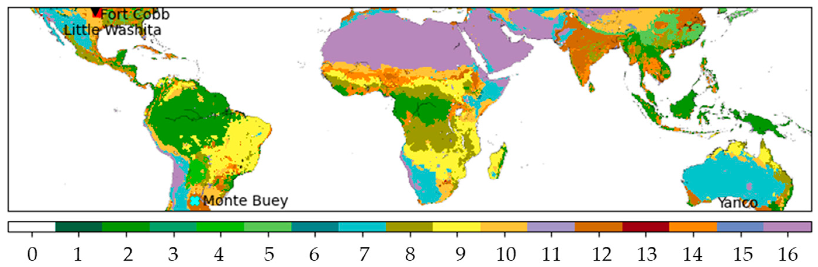
| Site Name | Longitude, Latitude | IGBP Land Cover | Climate |
|---|---|---|---|
| Fort Cobb | 35.36°N, 98.55°W | Grasslands | Temperate |
| Little Washita | 34.97°N, 97.97°W | Grasslands | Temperate |
| Monte Buey | 32.96°S, 62.52°W | Croplands | Arid |
| Yanco | 34.8°S, 146.11°E | Croplands/Grasslands | Semi-arid |
| Land Cover Type | Mean VWC (kg/m2) | Mean SM (cm3/cm3) | RMSE (cm3cm−3) | ubRMSE (cm3cm−3) | MAE (cm3cm−3) | |
|---|---|---|---|---|---|---|
| Barren/Sparsely Vegetated | 0.01 | 0.0708 | 0.0010 | 0.021 | 0.016 | 0.014 |
| Open Shrublands | 0.44 | 0.1047 | 0.0045 | 0.037 | 0.031 | 0.026 |
| Grasslands | 1.01 | 0.1628 | 0.0121 | 0.050 | 0.043 | 0.040 |
| Croplands | 2.00 | 0.2478 | 0.0150 | 0.051 | 0.045 | 0.039 |
| Savannas | 2.77 | 0.1731 | 0.0113 | 0.054 | 0.048 | 0.045 |
| Cropland/Natural Vegetation | 3.57 | 0.2358 | 0.0118 | 0.056 | 0.051 | 0.046 |
| Woody Savannas | 4.28 | 0.2653 | 0.0117 | 0.059 | 0.050 | 0.049 |
| Deciduous Broadleaf Forest | 9.31 | 0.2472 | 0.0104 | 0.066 | 0.056 | 0.056 |
| Mixed Forest | 9.49 | 0.3809 | 0.0054 | 0.072 | 0.059 | 0.058 |
| Evergreen Broadleaf Forest | 15.99 | 0.4257 | 0.0024 | 0.079 | 0.062 | 0.066 |
Disclaimer/Publisher’s Note: The statements, opinions and data contained in all publications are solely those of the individual author(s) and contributor(s) and not of MDPI and/or the editor(s). MDPI and/or the editor(s) disclaim responsibility for any injury to people or property resulting from any ideas, methods, instructions or products referred to in the content. |
© 2023 by the authors. Licensee MDPI, Basel, Switzerland. This article is an open access article distributed under the terms and conditions of the Creative Commons Attribution (CC BY) license (https://creativecommons.org/licenses/by/4.0/).
Share and Cite
Liu, Q.; Zhang, S.; Li, W.; Nan, Y.; Peng, J.; Ma, Z.; Zhou, X. Using Robust Regression to Retrieve Soil Moisture from CyGNSS Data. Remote Sens. 2023, 15, 3669. https://doi.org/10.3390/rs15143669
Liu Q, Zhang S, Li W, Nan Y, Peng J, Ma Z, Zhou X. Using Robust Regression to Retrieve Soil Moisture from CyGNSS Data. Remote Sensing. 2023; 15(14):3669. https://doi.org/10.3390/rs15143669
Chicago/Turabian StyleLiu, Qi, Shuangcheng Zhang, Weiqiang Li, Yang Nan, Jilun Peng, Zhongmin Ma, and Xin Zhou. 2023. "Using Robust Regression to Retrieve Soil Moisture from CyGNSS Data" Remote Sensing 15, no. 14: 3669. https://doi.org/10.3390/rs15143669