Research on Dynamic Deformation Laws of Super High-Rise Buildings and Visualization Based on GB-RAR and LiDAR Technology

Abstract

It is well-known that structures composed of super high-rise buildings accumulate damages gradually due to ultra-long loads, material aging, and component defects. Thus, the bearing capacity of the structures can be significantly decreased. In addition, these effects may cause inestimable life and property losses upon strong winds, earthquakes, and other heavy loads. Hence, it is necessary to develop real-time health monitoring methods for super high-rise buildings to deeply understand the running state during operation, timely discover potential safety potentials, and to provide reference data for reinforcement design. Along these lines, in this work, the built super high-rise buildings (Yunding Building) and super high-rise buildings (the Main Tower of the Shandong International Financial Center), under construction, were selected as the research objects. The overall dynamic deformation laws of super high-rise buildings were monitored by using ground-based real aperture radar (GB-RAR) technology for its advantages in non-contact measurement, remote monitoring, and real-time display of observation results. Denoising of the observation data was also carried out based on wavelet analysis. The visualization of the space state of the Yunding Building was realized based on handheld LiDAR technology. From the acquired results, it was demonstrated that the measuring accuracy of GB-RAR could reach the submillimeter level, while the noises under a natural state of wavelet analysis were eliminated well. The maximum deformation values of the Yunding Building and the Main Tower of Shandong International Financial Center under their natural state were 9.63 mm and 16.46 mm, respectively. Under sudden wind loads, the maximum deformation of the Yunding Building could be as high as 895.79 mm. The overall motion state switched between an S-shaped pattern, hyperbolic-type, and oblique line, presented the characteristics of nonlinear elastic deformation.

1. Introduction

With the rapid economic development and accelerating urbanization in China, an enhanced number of people are gathered in cities. As a consequence, the maintenance of the harmonious development of the population with land, energy, and the environment has become one of the major problems that have to be solved during continuous economic development. High-rise and super high-rise buildings have incomparable advantages in terms of full use of land resources, whereas urbanization and concentration of urban activities can also be promoted. By the end of 2022, the number of completed and capping super high-rise buildings over 200 m high reached 1034, ranking the top in the world for 27 successive years. Moreover, the uniqueness and size of the structural designs also set new records. The construction of structures of such ultra-high, ultra-scale, and unconventionally designed building groups may gradually accumulate damages during operation over decades, and even hundreds of years, due to ultra-long loading, material aging, component defects, etc. As a result, the bearing capacity of these structures will inevitably be decreased and may cause inestimable life and property losses upon strong winds, earthquakes, and other heavy loads [1,2,3]. The physical structures of super high-rise buildings may change once the deformation reaches a limit, thus influencing their normal functions and service life. Hence, it is of utmost importance to carry out health monitoring of super high-rise buildings to guarantee their safe operation and discover potential safety potentials in a timely manner.

The commonly available deformation monitoring methods of super high-rise buildings include the total-station instrument method [4], accelerometer sensors [5,6,7], digital vertimeters [8], and global navigation satellite system (GNSS) technology [9,10,11,12,13]. Among them, the total-station instrument method refers mainly to the installation of a prism on some characteristic points of the buildings and the determination of the deformation properties of the buildings by observing the prism. However, this method has a relatively low sampling frequency of monitoring and cannot realize real-time dynamic monitoring. The accelerometer sensor mainly acquires the vibration acceleration pattern of the buildings by using a network of sensors installed on the buildings and acquires displacement changes of the buildings by processing the acceleration data. Nonetheless, the application of these two methods requires direct contact with buildings before measurement. It is relatively difficult to install prism or sensors on some special buildings (e.g., super high-rise buildings), thus failing to provide accurate deformation characteristics that significantly affect the accuracy of the monitoring. A digital vertimeter uses the prepared holes of building floors as the installation channel and acquires deformation characteristics by recording the oscillation laws of the buildings. However, it is easy to be influenced by construction factors and wind load during monitoring. On top of that, none of the above-mentioned three methods can realize continuous real-time dynamic monitoring of super high-rise buildings. With the gradual improvement in positioning accuracy of the GNSS technology and the gradual maturity of the processing mode, GNSS has begun to be extensively applied to the deformation monitoring of super high-rise buildings. Representative projects include the deformation monitoring of Guangzhou Tower [14] and Tianjin 117 Tower [15] based on the GNSS technology. However, tower crane operation may shield GNSS signals, and the multi-path effect caused by steel structures, as well as vibration and wind loads, may generate serious noises. As a result, GNSS signals may contain a lot of noise data, thus seriously influencing the accurate extraction of deformation characteristics of super high-rise buildings. Although the above-mentioned four methods can only reflect the deformation characteristics of buildings through several characteristic points, effective overall monitoring and analysis of the buildings cannot be made. Moreover, all the above-mentioned measurement methods require physical contact with buildings, which causes potential safety hazards during the monitoring of buildings under construction or on some special buildings.

Interferometric synthetic aperture radar (InSAR) is increasingly used in deformation monitoring due to its comparative advantages of high monitoring accuracy, wide monitoring range, 24 h/d, and all-weather monitoring [16]. Li Ruifeng et al. monitored the Wuhan Greenland Center through InSAR technology and proved that InSAR technology could detect micro-deformation of super high-rise buildings. As a result, the abnormal deformation can be discovered, analyzed, and studied timely. Hence, countermeasures could be adopted timely to prevent accidents [17]. Wu et al. measured the deformation of high-rise buildings in urban areas by using the persistent scatterer InSAR (PSInSAR) and analyzed spatial and temporal features of building deformation by combining the 3D model of Google Earth [18]. Compared with traditional methods, InSAR is superior for non-contact operation, low cost, and high spatial resolution. Limited by the carrying platform, InSAR also has some drawbacks. Due to the insufficient temporal resolution, it is impossible to obtain deformation information in a short period. Moreover, it has some geometric distortion and atmospheric delay. Ground-based interferometric synthetic aperture radar (GB-InSAR) technology is born at the right moment. This technology can overcome the disadvantages of satellite-borne InSAR and realize high-frequency data collection and high-precision deformation monitoring [19]. With the high measuring precision, small influences by atmospheric delay, high sampling frequency, and contactless measuring, ground-based radar technology has been extensively applied to the field of deformation monitoring. Particularly, Tapete et al. integrated the GB-InSAR and ground 3D laser scanning technology to generate 3D interference point clouds, which were successfully used to interpret the overall displacement deformation of 3D space of Rome Forum ruins in Italy [20]. Marichsio et al. carried out a comparative study of the dynamic changes of the Leaning Tower of Pisa in Italy under natural and artificial conditions by using the GB-InSAR technology. The acquired experimental results proved that GB-InSAR could reach the displacement measuring accuracy of 0.01 mm. The authors also verified that GB-InSAR can realize simple, convenient, and effective monitoring of the health state of linear building structures [21].

Luzi et al. used a ground-based true aperture radar (GB-RAR) interferometer to monitor the vibration of buildings. The monitoring results show that under the premise of good monitoring results, GB-RAR can be used to deform from microns to centimeters [22]. Zhou Lu et al. used GB-RAR technology to analyze and process the monitoring data of the Wuhan Greenland Center (WGC), and proposed a set of monitoring and analysis techniques for dynamic characteristics of super high-rise buildings based on GB-RAR and wavelet analysis [23]. Montuori et al. combined GB-RAR, ground-based synthetic aperture radar (GB-SAR) and spaceborne InSAR. This method can estimate the dynamic characteristics of buildings and monitor the deformation of the surrounding area at different spatiotemporal scales [24]. Although the works in the literature on longitudinal architecture, like buildings and towers, have accumulated some results, a systematic study on the underlying deformation mechanism and motion characteristics of super high-rise buildings over 300 m high is still missing. In addition, the modeling accuracy of ground-based radar technology is relatively low when considering the accuracy of data acquisition, cost, and feasibility of scene implementation, thus, three-dimensional laser scanning technology can be used for modeling. Cheng Yugang et al. used a ground 3D laser scanner to measure a Soviet-style courtyard, drew two-dimensional drawings with the point cloud data, and constructed a virtual scene model and texture mapping with 3ds Max according to the two-dimensional mapping, thus completing the three-dimensional reconstruction of the courtyard [25]. Zou Jingui et al. proposed a fusion method of ground-based synthetic aperture radar and ground-based three-dimensional laser scanning (TLS) data, which fused a two-dimensional interferogram with a three-dimensional laser point cloud to generate a three-dimensional interferogram, which could demonstrate the deformation state of the measured object from a three-dimensional perspective [26].

To this end, the Yunding Building and Main Tower of Shandong International Financial Center (under construction) (hereinafter referred as the Main Tower) were chosen as the research objects in this work. GB-RAR was used to monitor the deformation characteristics of super high-rise buildings in their natural state. The noises in the signals were removed by wavelet analysis. The visualization of the space state of the super tall building is realized by LiDAR technology. Valuable dynamic deformation information about the displacement, amplitude, and acceleration of the buildings was extracted, and the health conditions of the super high-rise buildings were thoroughly evaluated.

2. Research Methods

The essence of the GB-RAR deformation data analysis is the deformation at future moments relative to the initial moment. Deformation data at multiple moments formed time series of deformation characteristics like acceleration, displacement, and amplitude. The core principle was introduced as follows.

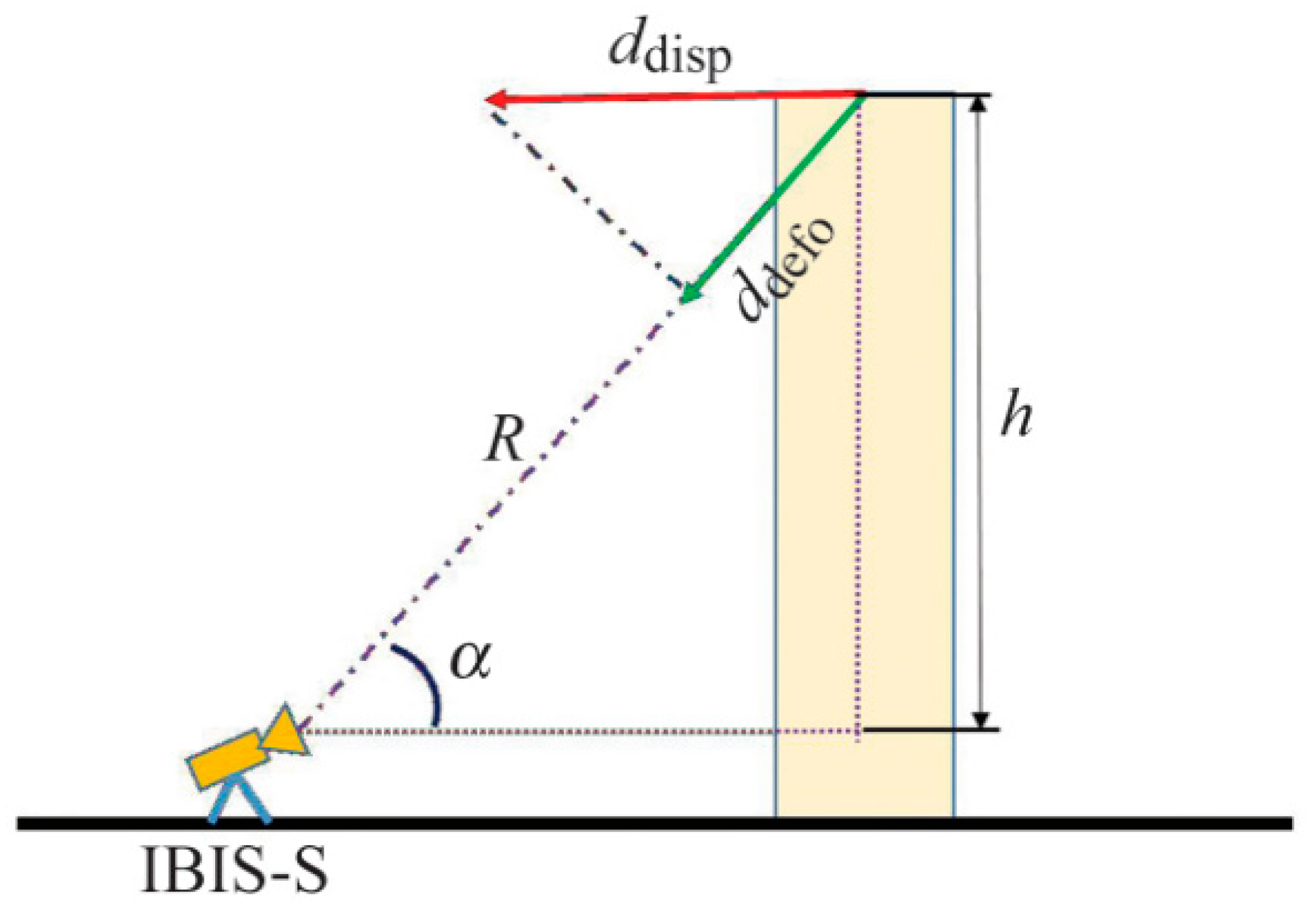
2.1. Differential Interference Processing

Compared with spaceborne SAR, GB-RAR belongs to zero-base line observation. Assuming that the distance between GB-RAR and the target point is R₁ when no deformation occurs, the phase composition of the point after radar measurement can be expressed as:

$${\phi }_1=-\frac{4\pi }{\lambda }{R}_1+{\phi }_{atm1}+{\phi }_{noise1}$$

(1)

where $\lambda$ is the wavelength, ${\phi }_{atm1}$ refers to the atmospheric delay phase at measurement under no deformation, and ${\phi }_{noise1}$ denotes the noise phase at measurement under no deformation. After the deformation occurs, the distance between GB-RAR and the measured target point is R₂, and the phase composition of the point after radar measurement can be expressed as:

$${\phi }_2=-\frac{4\pi }{\lambda }{R}_2+{\phi }_{atm2}+{\phi }_{noise2}$$

(2)

where $\lambda$ is the wavelength, ${\phi }_{atm2}$ refers to the atmospheric delay phase at measurement after the occurrence of deformation, ${\phi }_{noise2}$ stands for the noise phase at measurement after the occurrence of deformation. The data of twice measurement interfered and the interferometric phase of target point can be expressed as follows:

$$\varphi ={\phi }_2-{\phi }_1=-\frac{4\pi }{\lambda }(R_2-R_1)+({\phi }_{atm2}-{\phi }_{atm1})+({\phi }_{noise2}-{\phi }_{noise1})$$

(3)

The sampling frequency of this experiment was relatively high. Given a high signal-to-noise ratio (SNR), it can be generally assumed that the atmospheric states were consistent. Hence, ${\phi }_{atm1}={\phi }_{atm2}$ and ${\phi }_{noise1}={\phi }_{noise2}$. The visual deformation can be expressed as follows: $\Delta d=R_2-R_1$.

In other words:

$$\Delta d=-\frac{4\pi }{\lambda }\varphi$$

(4)

The goal of this monitoring process is to acquire horizontal displacement information on buildings. However, instruments measure the visual displacement directly. Therefore, an assembly projection of visual displacement is essential to acquire the horizontal component, which is the horizontal displacement of buildings:

$$d_{disp}=\frac{d_{defo}}{\mathit{cos}\alpha }$$

(5)

$d_{defo}$ refers to visual displacement and $\alpha$ is the included angle between the horizontal direction and vision line of the radar. The relationship between visual displacement and horizontal displacement is shown in Figure 1.

2.2. Wavelet Denoising

2.2.1. Wavelet Denoising Principle

To decrease the influence of noises and improve SNR, wavelet denoising analysis was applied. The essence of wavelet threshold denoising is to obtain an approximate value $\tilde{f}\left(t\right)$ of the real signals $f(t)$ after wavelet processing of the noise-containing function $S(t)$. In other words, $\tilde{f}\left(t\right)$ is the optimal estimation value of $f(t)$ under some conditions. The specific algorithm can be expressed as follows:

Suppose the noise-containing function $S\left(t\right)$ is:

$$S(t)=f(t)+\sigma \times e(t)$$

(6)

where $f(t)$ is the real signal, $e\left(t\right)$ refers to various sources of noise, $\sigma$ denotes the noise level, and t represents the equivalent time interval. The discrete signals $f\left(n\right)$ of n points ($\mathrm{t}=1,2,\cdots \cdots ,n-1$) could be acquired through a discrete sampling of $f\left(t\right)$. Wavelet transformation of discrete signals was carried out:

$$W_f(m,b)=2^{-\frac{m}{2}}\sum _{n=0}^{N-1}f\left(n\right)\Psi \left(2^{-m}-b\right),\left(m,b\in Z\right)$$

(7)

where $W_f\left(m,b\right)$ is the coefficient gained after the wavelet transformation. In practical calculations, the above formula incurs very complicated computation, and the wavelet function $\Psi \left(t\right)$ has no specific expression. Hence, the recursion of the wavelet transformation can be realized by the following method [23,24]:

$$\begin{array}{c}{S}_f\left(m+1,b\right)=S_f\left(m,b\right)\times h\left(m,b\right)\\ S_f\left(m+1,b\right)=S_f\left(m,b\right)\times g\left(m,b\right)\end{array}$$

(8)

Here, $h (m,b) and g (m,b)$ are the two filters of the wavelet transform. The corresponding reconstruction formula was as follows:

$$S_f\left(m-1,b\right)=S_f\left(m,b\right)\times h\left(m,b\right)+W_f\left(m,b\right)\times g\left(m,b\right)$$

(9)

Since there is no obvious expression, a recursive implementation method of wavelet transform has appeared.

The basic principle of wavelet threshold denoising can also be summarized as that it can achieve the optimal approximation on the basis of the minimum mean square error and can obtain better visual effects, so it has been deeply studied and widely used. This method is mainly used in the case of mixed white noise in the signal. According to the ability of white noise in the wavelet transform domain, it mainly focuses on the characteristics of low-amplitude wavelet coefficient. On the basis of any orthogonal, the transformation of white noise is still white noise, and the amplitude is the same. The wavelet coefficient below the threshold can be set to zero, and the signal noise can be effectively suppressed. This method obtains the approximate optimal estimate of the original signal, and has wide applicability, and is also the most commonly used method in wavelet denoising.

2.2.2. Selection of Threshold

The selection of the threshold in wavelet denoising is closely related to the ultimate effect. If the threshold is too small, the denoised signals still contain excessive noises. On the contrary, if the threshold is too high, the denoised signals may lose some useful signal data, resulting in distortion of reconstructed signals. Some common threshold selection methods were introduced in the following text.

(1)

Fixed threshold (sqtwolog)

The fixed threshold is also called the universal threshold and it can be expressed as follows:

$$\lambda =\sigma \sqrt{2\mathit{ln}N}$$

(10)

where $\sigma$ refers to the standard deviation of noises.

(2)

The unbiased risk estimation threshold (rigsure)

Unbiased risk estimation threshold is an adaptive threshold selection method based on the Stein unbiased likelihood estimation principle. The process is as follows:

First, absolute values of all elements in the signals were collected and the square value of these absolute values was calculated. A new sequence was gained through re-sequencing:

$$f\left(k\right)=sort{\left(\left|S\right|\right)}^2,\left(k=\mathrm{0,1},2,......,N-1\right)$$

(11)

where sort refers to the sequence. Suppose the square root of the nth element of the threshold $f\left(k\right)$ is:

$${\lambda }_n={\sigma }_{\mu }\sqrt{f\left(n\right)},\left(k=\mathrm{0,1},2,......,N-1\right)$$

(12)

The risk formed by this threshold is as follows:

$$Rish\left(n\right)=\left[N-2n+{\sum }_{j=1}^{n}f(j)+(N-n)f(N-n)\right]/N$$

(13)

According to the Rish(n) curve, if $n_{min}$ is the corresponding value of the minimum risk point, there’s ${\lambda }_n={\sigma }_{\mu }\sqrt{f(n_{min})}$.

(3)

Heuristic threshold (heuresure)

The heuristic threshold is a threshold method between a fixed threshold and an unbiased risk estimation threshold. It is also a selection method for the optimum prediction of the variable threshold.

It can be expressed as follows:

$$\begin{array}{c}crit=\sqrt{\frac{1}{N}{\left(\frac{\mathit{ln}N}{\mathit{ln}2}\right)}^3}\\ eta=\left[{\displaystyle \sum _{j=1}^N}{\left|S_j\right|}^2-N\right]/N\end{array}$$

(14)

where crit > eta, the fixed threshold was applied for denoising. Otherwise, the smaller threshold of fixed threshold and unbiased risk estimation threshold was used as the denoising standard.

2.2.3. Evaluation Standards

There are various wavelet denoising methods. Due to different selections of influencing factors, such as the number of decomposition layers and the wavelet function, different denoising effects may be produced. In the following text, five common evaluation indicators were introduced.

(1)

Root mean square error (RMSE)

The RMSE can explain the degree of dispersion between two signals and also reflects signal distortion. RMSE can be defined as follows:

$$RSME=\sqrt{\frac{1}{n}\sum _n{\left[f\left(n\right)-\widehat{f}\left(n\right)\right]}^2}$$

(15)

where f(n) is the original signal and $\widehat{f}(n)$ denotes the denoised signal. The existence of a higher RMSE value indicates that the deviation between the two signals is big and the denoising effect is poor. In striking contrast, a smaller RMSE value reflects a reduced deviation between the two signals and a better denoising effect.

(2)

SNR

SNR refers to the signal-to-noise ratio. Its formula is as follows:

$$SNR=10\times {\mathit{log}}_{10}\left(powe{r}_{signal}/powe{r}_{noise}\right)$$

(16)

where $powe{r}_{signal}=\frac{1}{n}(f(n){)}^2$ and $powe{r}_{noise}=\frac{1}{n}{\left(f(n)-\widehat{f}(n)\right)}^2$.$f(n)$ represents the original signal and $\widehat{f}(n)$ refers to the denoised signal. A higher SNR value indicates that more noises in the signals are removed, and the denoising effect is relatively ideal. On the contrary, the lower SNR value reflects that few noises in signals are removed, and the denoising effect is relatively poor.

(3)

Cross-correlation coefficient (R)

The cross-correlation coefficient refers to the correlation between the denoised reconstruction signal and the original signal. It can be expressed as follows:

$$R=\frac{\mathit{cov}\left(f\left(n\right),\widehat{f}\left(n\right)\right)}{{\sigma }_f{\sigma }_{\widehat{f}}}$$

(17)

(4)

Smoothness index (r)

The smoothness index refers to the ratio between the square sums of differentials between the denoised reconstruction signal and the original signal. It can be expressed as follows:

$$r={{\displaystyle \sum _{n=1}^{n-1}}\left[\widehat{f}\left(n+1\right)-\widehat{f}\left(n\right)\right]}^2/{{\displaystyle \sum _{n=1}^{n-1}}\left[f\left(n+1\right)-f\left(n\right)\right]}^2$$

(18)

where $f(n)$ represents the original signal and $\widehat{f}\left(n\right)$ denotes the denoised signal. Generally speaking, the smoothness index value is smaller if the signal is smooth and the denoising effect is better.

(5)

Sample Standard Deviation (SSD)

Considering the usefulness of RMSE for evaluating the quality of denoised signals, a lower RMSE can be obtained when the original signal is very similar and very close to the denoised signal, but the denoised signal should be somewhat different from the original signal. So we introduce a standard measurement of sample standard deviation (SSD) to describe the quality of signal denoising.

$$SSD=\sqrt{\frac{1}{n-1}\left(\sum _n{\left[f\left(n\right)-\overline{f}\left(n\right)\right]}^2\right)}$$

(19)

where $f(n)$ represents the signal, and $\overline{f}\left(n\right)$ represents the mean value of the reorganization signal. Generally speaking, the smaller the sample standard deviation, the smaller the deviation of the signal, and the better the denoising effect.

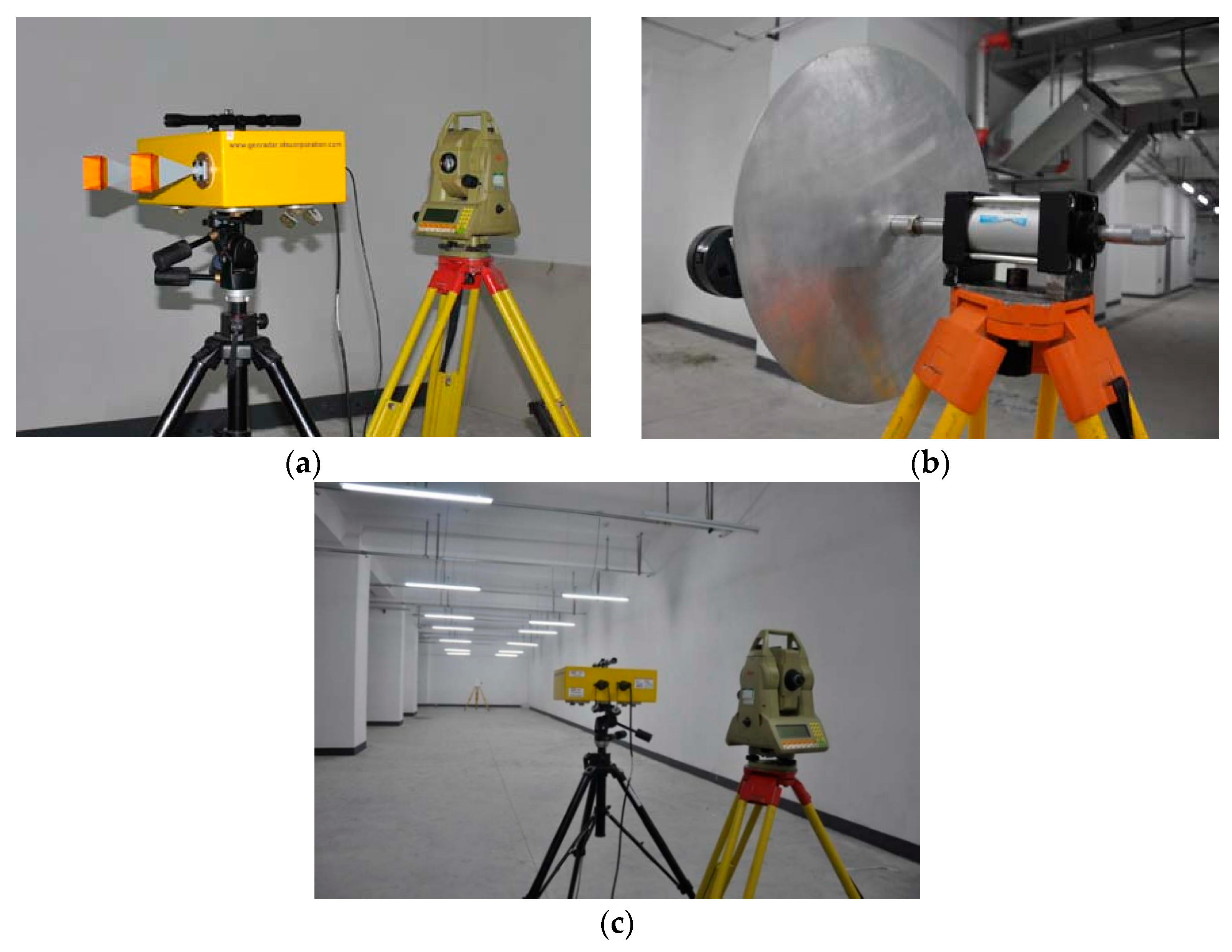
3. Accuracy Verification Experiment

It is necessary to evaluate the measurement accuracy of the IBIS-FS microdeformation monitoring system before the field engineering test. The equipment used in this calibration experiment includes a dial gauge, reflector, IBIS-FS micro-deformation monitoring system, and TCA2003 measuring robot (Figure 2a).

Among them, the nominal displacement monitoring accuracy of the IBIS-FS instrument is 0.1~0.01 mm. The dynamic data acquisition mode was adopted in the experiment, the sampling frequency was 100 Hz, and the instrument was set up in the direction of the observation target (front reflector). The front reflector is a circular plate made of aluminum alloy with a thickness of 3 mm and a radius of 22 cm (Figure 2b). The nominal accuracy of the distance measurement of the TCA2003 total station is 1 mm + 1 ppm, and the reading value of the total station can reach 0.1 mm in the accuracy detection test. The instrument precision testing environment is a closed basement, which is not ventilated, and the temperature is relatively stable, and the influence of human and natural environment disturbance is reduced to a certain extent. The test site is shown in Figure 2c.

This paper identifies the test principle as follows: the front-end reflector is taken as the observation target, the observation target is connected to the dial meter, which is slightly adjusted to make the observation target move correspondingly, and the displacement change of the target is observed synchronously with the IBIS system and TCA 2003. The data of the micrometer trimming section, IBIS system displacement monitoring data, and TCA2003 displacement monitoring results are compared and analyzed.

Through data processing, the displacement monitoring results of the IBIS-FS micro-deformation monitoring system and TCA2003 measuring robot in tests 1~3 are obtained, respectively. Because the accuracy of the dial gauge reaches ±0.004 mm, the adjustment distance of the dial gauge is used as the real displacement data in this test, and some of the measurement accuracy characterization data are shown in

Table 1. Comparison table of monitoring results between the dial meter, IBIS system and TCA2003.

Name	Number of Adjustments	IBIS Monitoring (mm)	TCA2003 Monitoring (mm)	Dial Meter Adjustment (mm)	IBIS Error (mm)	TCA2003 Error (mm)
Experiment 1	1	1.0274	1	1	0.0274	0
	2	0.9786	1.02	1	−0.0214	0.02
	3	−0.9876	−1.02	−1	−0.0124	0.02
	4	−1.0502	−0.98	−1	0.0502	−0.02
Experiment 2	1	0.4652	0.4	0.5	−0.0348	−0.1
	2	0.5187	0.47	0.5	0.0187	−0.03
	3	0.4634	0.58	0.5	−0.0366	0.08
	4	−0.4875	−0.48	−0.5	−0.0125	−0.02
	5	−0.5248	−0.5	−0.5	0.0248	0
	6	−0.5347	−0.5	−0.5	0.0347	0
Experiment 3	1	0.2157	0.17	0.2	0.0157	−0.03
	2	0.2034	0.18	0.2	0.0034	−0.02
	3	0.0982	0.15	0.1	0.0022	0
	4	0.2048	0.25	0.2	0.0048	0.05
	5	−0.1885	−0.2	−0.2	−0.0115	0
	6	−0.1918	−0.18	−0.2	−0.0082	−0.02
	7	−0.209	−0.22	−0.2	0.009	0.02
	8	−0.2234	−0.18	−0.2	0.0234	−0.02

.

It can be seen from Table 1 that in experiment 1, the maximum displacement monitoring error of IBIS was 0.0502 mm, and the maximum displacement monitoring error of TCA2003 was ±0.02 mm. In experiment 2, the maximum displacement monitoring error of IBIS was −0.0366 mm, and the maximum displacement monitoring error of TCA2003 was −0.10 mm. In experiment 3, the maximum displacement monitoring error of IBIS was 0.0234 mm, and that of TCA2003 was 0.05 mm.

It can be seen from the above that, based on this precision detection test, the maximum error of IBIS displacement monitoring was 0.05 mm, and the median error was 0.0165 mm. Moreover, the stability of the displacement monitoring results was good, and the displacement monitoring accuracy of the IBIS system was better than that of the TCA2003 measuring robot.

4. Deformation Monitoring Test of Super High-Rise Buildings

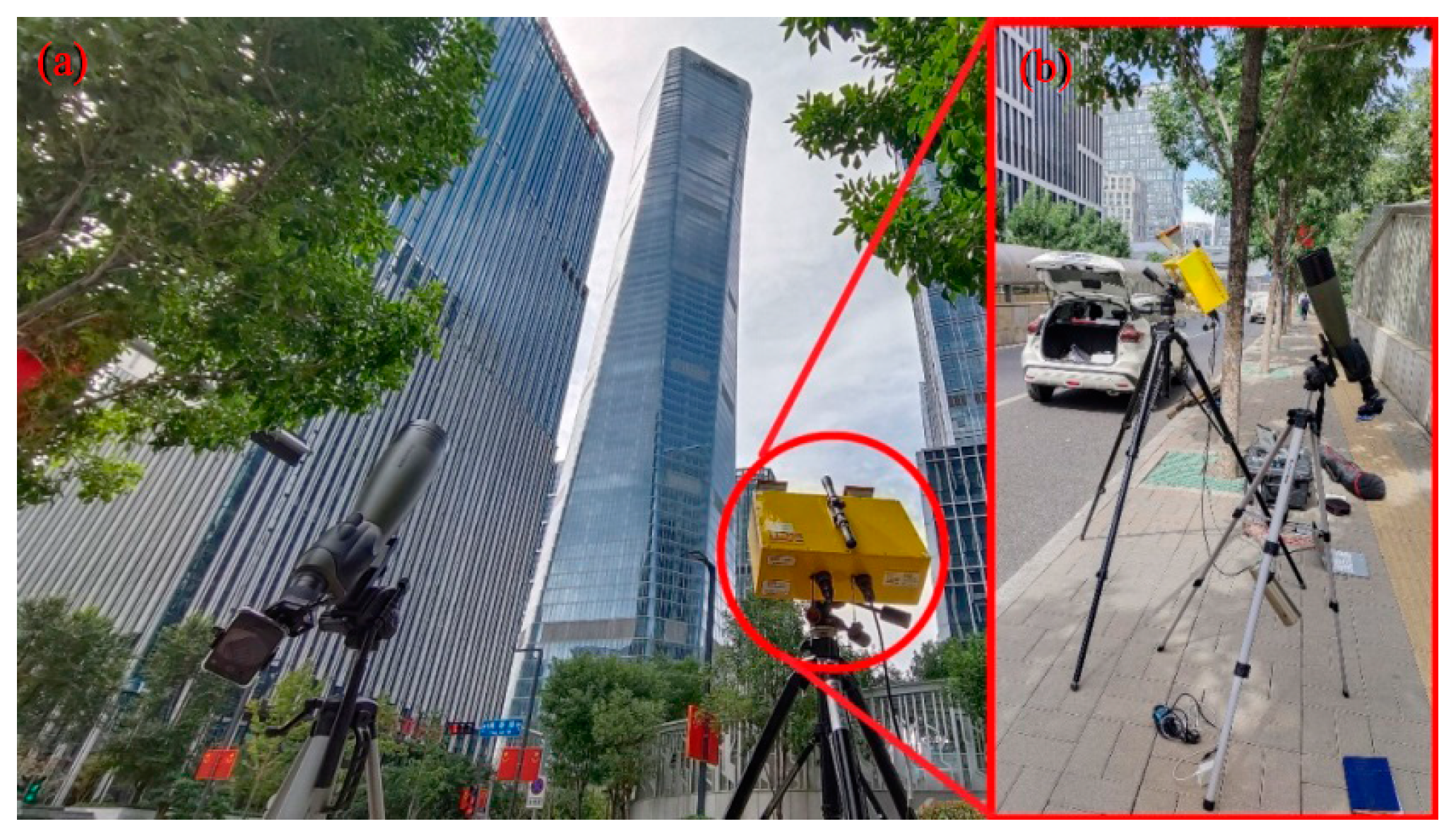
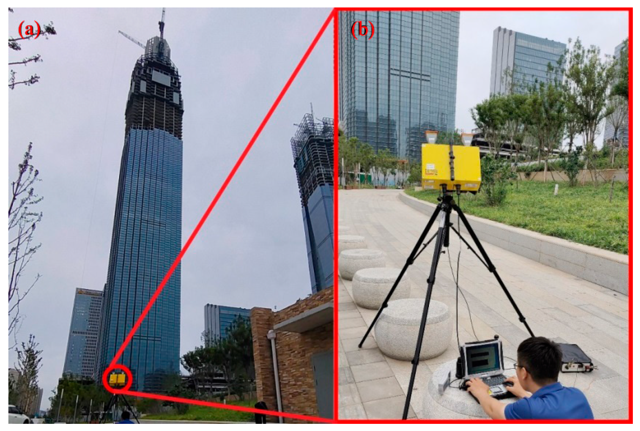
4.1. Experimental Subjects

The Jinan Yunding Building is located in CBD Hanyu Jingu in Jinan, and it has 69 floors, with a height of 339 m. More specifically, Floors 1–2 are the overhead hall, and the third floor is the hall of the Kempinski Hotel. Floors 4–50 are the business office area, and floors 51–69 are the Jinan Kempinski Hotel. The 69th floor is planned to be an all-around urban exhibition hall. A total of 67 express elevators are installed in the building, and the maximum speed of each elevator is 6.8 m/s.

The main body of the Yunding Building uses a reinforced concrete core-tube plus a concrete-filled steel tube frame. The total weight of the steel structure is more than 20,000 tons. The façade of the whole building is created by a full glass curtain wall, and a total of 9826 glass curtain walls are needed. Moreover, the weight of each glass curtain wall reaches more than 800 kg.

The Main Tower of Shandong International Financial Center is located in the Greenland Shandong National Financial Center. The designed number of floors is 88, and the building height is 428 m. It is currently under construction, and after completion, it is planned to be divided into offices, apartments, and hotel areas.

4.2. Experimental Scheme

In this work, high-precision dynamic deformation monitoring of the Jinan Yunding Building and the Main Tower was carried out by using an IBIS-S system. In particular, instruments were installed at S1, which is 180 m away from the southwest of the Yunding Building, and at S2, which is 210 m away from the southwest of the Main Tower (Figure 2 and Figure 3). The field data were collected by scanning the building with the IBIS-S system. The data were processed by IBIS-DV to obtain visual deformation information on the buildings. Finally, the horizontal displacement of the buildings was calculated through geometric transformation. Radar monitoring used a high-frequency data collection mode. Sampling frequencies were set at 30 Hz, 50 Hz, 80 Hz, and 100 Hz, respectively.

Continuous dynamic monitoring of the Yunding Building was implemented for about 3 h at 9:56, 25 September 2022. The monitoring process was introduced as follows:

(1)

9:56~10:24: monitored the building with the IBIS-S system at the sampling frequency of 100 Hz;

(2)

10:25~12:25: monitored the building with the IBIS-S system at the sampling frequency of 80 Hz;

(3)

12:26~12:56: monitored the building with the IBIS-S system at the sampling frequency of 100 Hz.

Continuous dynamic monitoring of the Main Tower was implemented for about 2.5 h at 15:23, 25 September 2022. The monitoring process was introduced as follows:

(1)

15:23~15:53: monitored the building with the IBIS-S system at the sampling frequency of 100 Hz;

(2)

16:00~16:30: monitored the building with the IBIS-S system at the sampling frequency of 80 Hz;

(3)

16:30~17:00: monitored the building with the IBIS-S system at the sampling frequency of 50 Hz;

(4)

17:00~17:30: monitored the building with the IBIS-S system at the sampling frequency of 30 Hz.

Monitoring diagrams of the Yunding Tower and the main tower are shown in Figure 3 and Figure 4.

5. Results and Discussion

The time when the radar began to collect data was used as the reference time of the data processing. Suppose the deformation of the building at this moment was 0. Another time quantum during the data processing was successively postponed based on this reference time. Besides, the data collected by GB-RAR were the sampling data of the echo frequency domain. Frequency spectra may have leakage during the staged analysis of such signals. To decrease the leakage of the frequency spectra, “windowing” is necessary for signals. Common window functions include the uniform window, Hannig window, Kasier–Bessel window, flat top window, and so on. In this work, the Hannig window was used according to data type and result selection; it can significantly decrease discontinuity caused by staged analysis and thereby decrease leakage. The data analysis was introduced in the following text.

5.1. Wavelet Denoising Analysis

5.1.1. Wavelet Noise Reduction Rule Parameter Combination Debugging

Take the signal data noise reduction results of feature points in Genting Building from 11:6 min 57 s to 11:11 min 57 s, as an example. For specific debugging, see

Table 2. Debug data of parameter combination of wavelet noise reduction rules.

Threshold Type	Threshold Function Type, Defined Threshold Rescaling Type, Wavelet Decomposition Layer Number, Wavelet Basis	R (Smoothness Index)	RMSE	SSD
heursure	s, sln, lev7, sym3	0.00925	0.14012	0.74264
	s, sln, lev7, sym8	0.00689	0.14083	0.74639
	s, sln, lev7, sym10	0.00701	0.14061	0.74523
	s, sln, lev1, sym3	0.25194	0.07988	0.42336
	s, sln, lev5, sym3	0.01033	0.13421	0.71131
	s, sln, lev6, sym7	0.00926	0.14012	0.74264
	s, sln, lev7, sym1	0.09723	0.15029	0.79654
	s, sln, lev7, sym2	0.01279	0.14495	0.76824
	s, sln, lev7, sym4	0.00781	0.14098	0.74719
	h, sln, lev7, sym3	0.02981	0.12421	0.65831
	h, mln, lev7, sym3	0.00621	0.34994	1.85467
	s, one, lev7, sym3	0.00605	0.22628	1.19928
	s, mln, lev7, sym3	0.00069	0.35112	1.86094
	s, one, lev7, sym3	0.00138	0.29108	1.54272
sqtwolog	s, sln, lev7, sym3	0.00712	0.15344	0.81323
	h, sln, lev7, sym3	0.02277	0.13012	0.68964
	s, mln, lev7, sym3	0.00053	0.35137	1.86226
	s, one, lev7, sym3	0.00066	0.32799	1.73835
Rigrsure	s, sln, lev7, sym3	0.05124	0.10059	0.53313
	h, sln, lev7, sym3	0.35572	0.08356	0.44287
	s, mln, lev7, sym3	0.01666	0.34349	1.82049
	s, one, lev7, sym3	0.00539	0.20022	1.06117

:

In this debugging, three threshold rules were selected, namely heursure, sqtwolog, and Rigrsure, and the effect of noise reduction is roughly observed by changing the definition of the threshold rescaling type, the number of wavelet decomposition layers and the wavelet basis. Because heursure is a threshold method between a fixed threshold and an unbiased risk estimation threshold, and it is also a way to select the threshold of the optimal predictor variable, debugging selects heursure as the threshold first. The debugging results show that when the threshold function type, threshold rescaling type, number of wavelet decomposition layers, and wavelet basis are fixed, r, RMSE and SSD when heursure is adopted are lower than those when sqtwolog and Rigrsure are adopted. From this we call heursure for subsequent wavelet denoising.

The selection of the number of decomposition layers of the small and medium waves also has a great influence on the effect of signal noise reduction. If the number of layers is too small, it will cause incomplete signal noise reduction; if the number of layers is too large, the effective signal will be ignored during quantization, resulting in signal distortion. Therefore, in the debugging process, it was found that heursure was selected as the threshold, soft threshold function s, sln (using the noise estimation rescaling based on the first level coefficient), when the wavelet basis was sym3, when the number of wavelet decomposition layers is 1, the signal noise reduction is incomplete, r is relatively large, which is represented by poor image smoothness and more burrs, and r gradually decreases with the increase of the number of layers. The image smoothness is improved and the burrs are reduced. However, with the increase of layers, the RMSE and SSD increases significantly and the signal is distorted when lev8. By comparing the data, it was found that the ideal noise reduction effect was achieved at lev7.

A commonly used wavelet base is wavelet denoising sym3, sym4, sym1, sym2, sym7, and sym8. The analysis of the debugging results showed that the RMSE and SSD of the sym3 wavelet function was the smallest and the denoising effect was the best, so the sym3 wavelet function was selected for denoising. Three types were used to define the threshold rescaling types: one (meaning no rescaling), sln (meaning rescaling with noise estimates based on first-order coefficients), and mln (meaning scaling with noise level correlation estimates). According to the analysis of the debugging results, although r (smoothness index) is greatly reduced when one or mln is called, RMSE and SSD are greatly increased, and the signal distortion is serious. However, both r, RMSE, and SSD can achieve better results when sln is called to define the threshold rescaling type. Therefore, compared with the above denoising experiment results, finally, sln was used to define the threshold rescaling type to denoise the monitoring data wavelet.

When selecting the types of threshold functions, we respectively called S (soft threshold function) and h (hard threshold function) to conduct noise reduction experiments. Compared with the results, it was found that although the RMSE and SSD of the signal after noise reduction of h (hard threshold function) was lower than S (soft threshold function), the signal distortion was small, but r (smoothness index) was greatly increased, resulting in more burrs in the image. The smoothness was poor, so the noise reduction effect of S (soft threshold function) was better than that of h (hard threshold function). By comparing the above denoising experiment results, a heursure criterion was adopted. S (soft threshold function) used the sym8 wavelet function in the 7th decomposition layer based on sln to denoise the monitoring data.

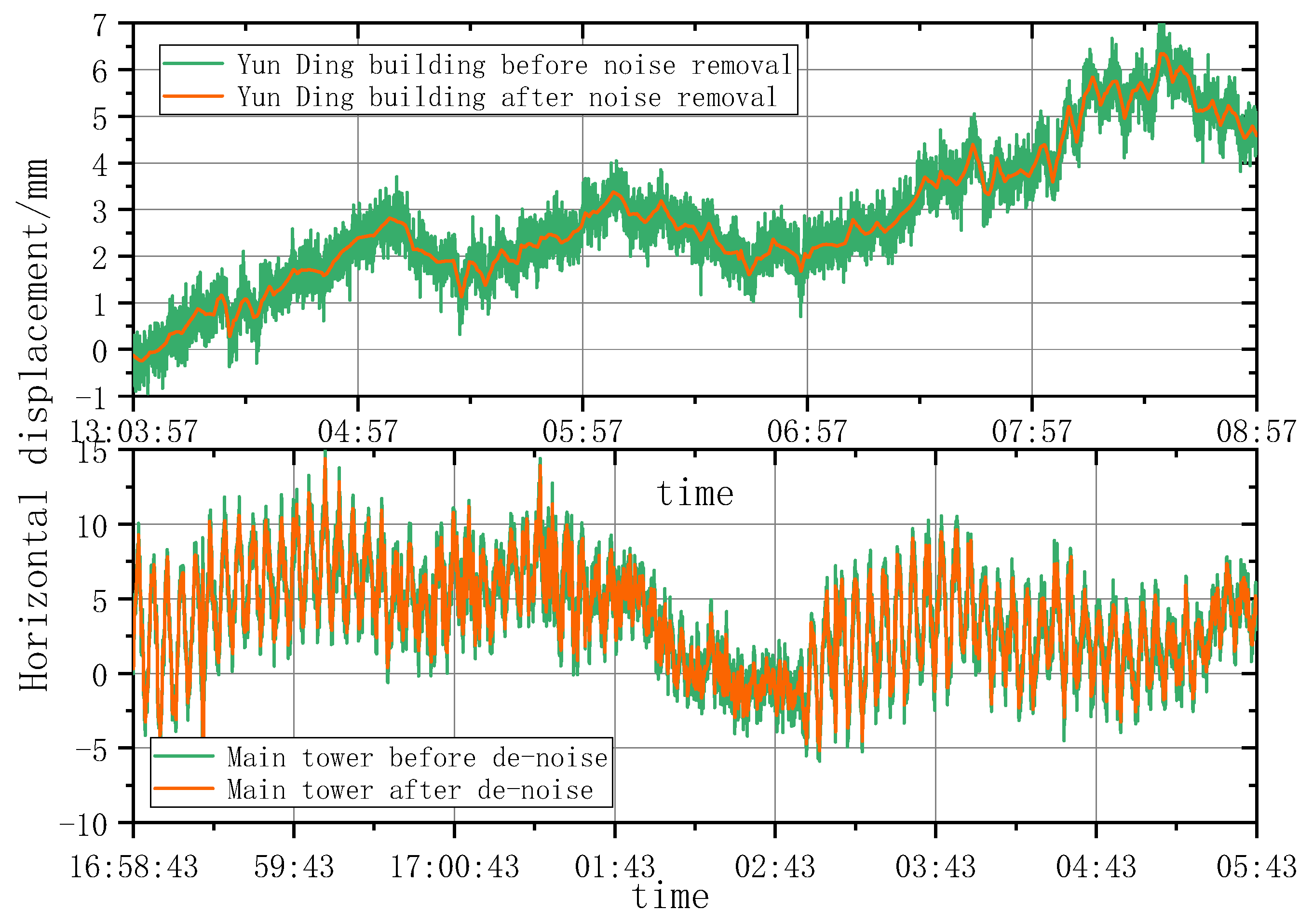
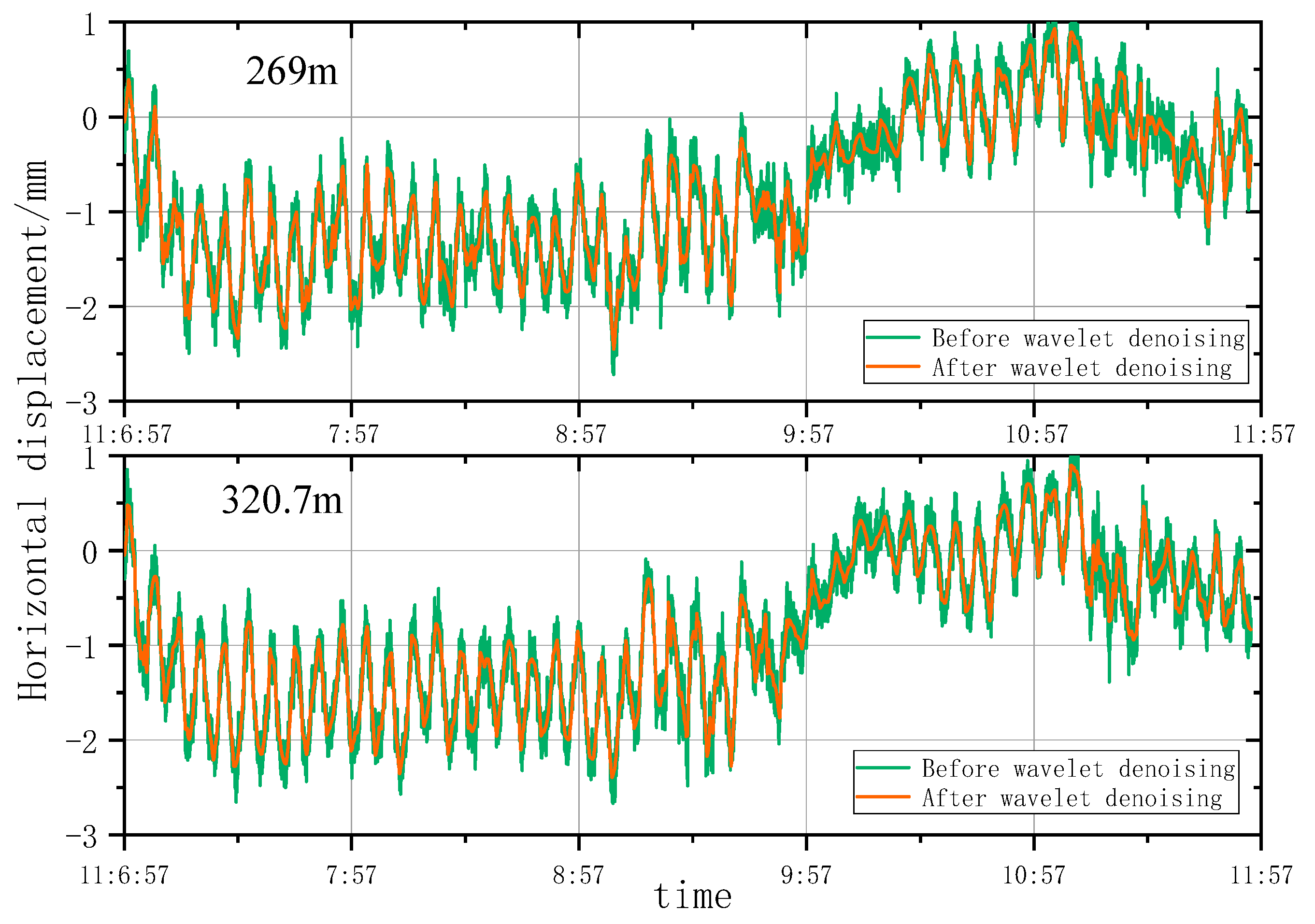
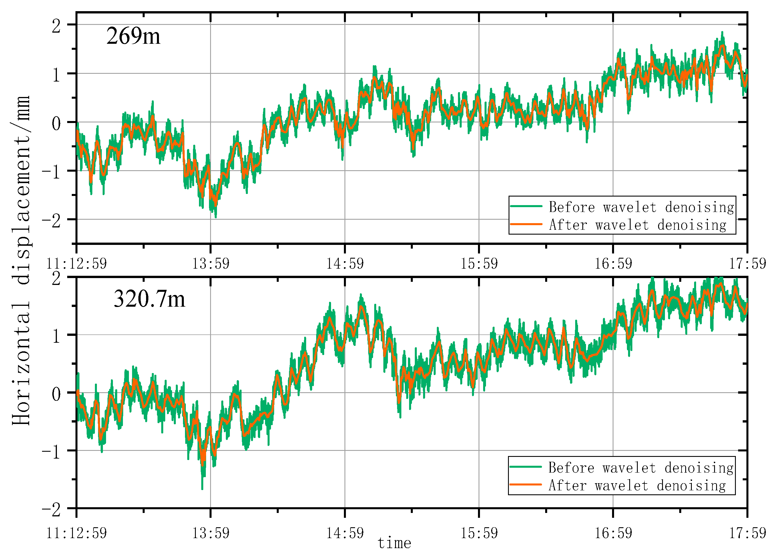
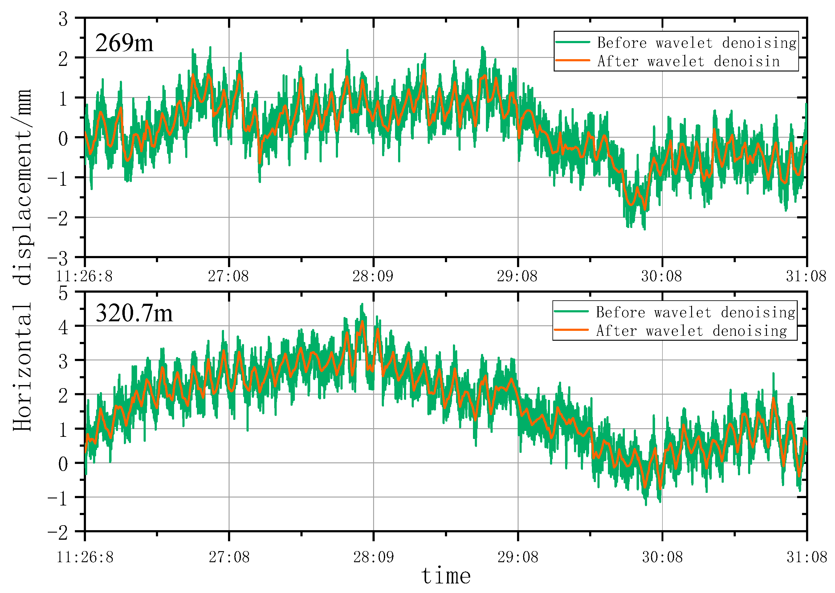
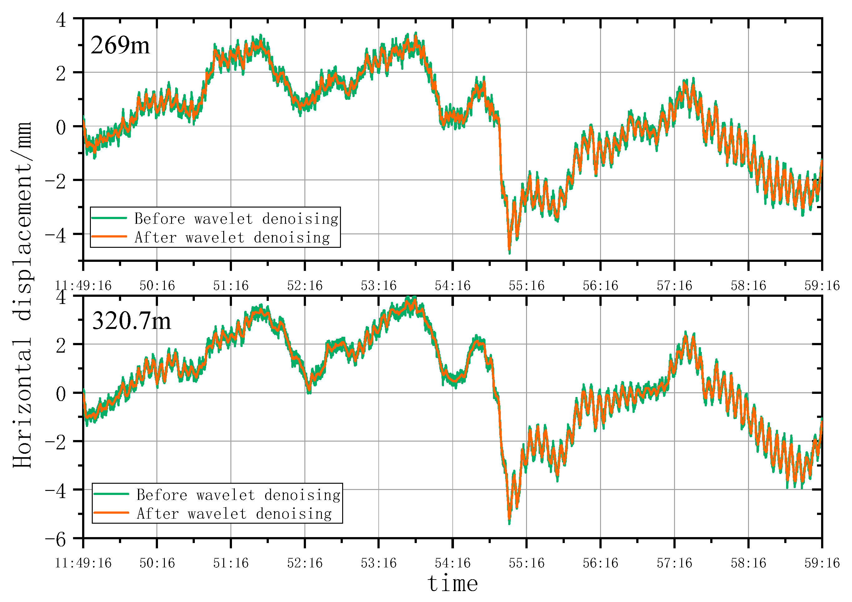
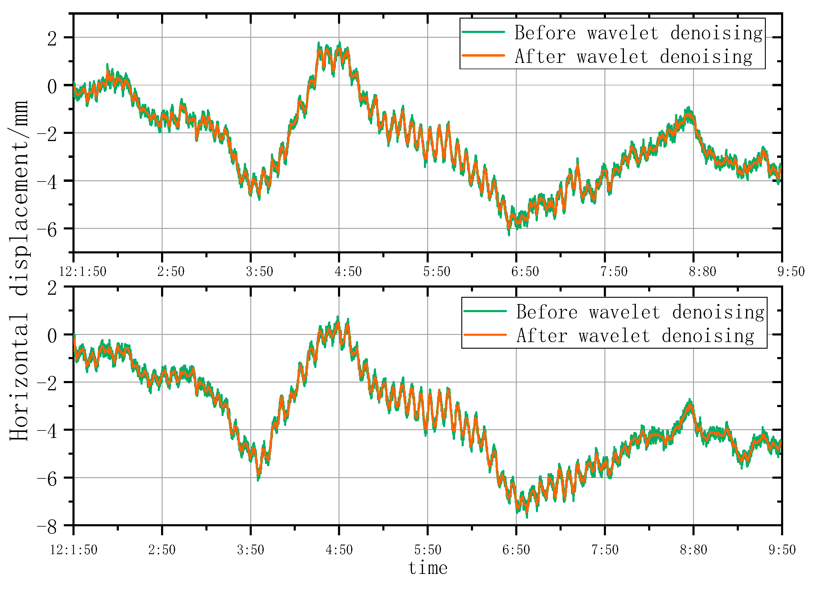
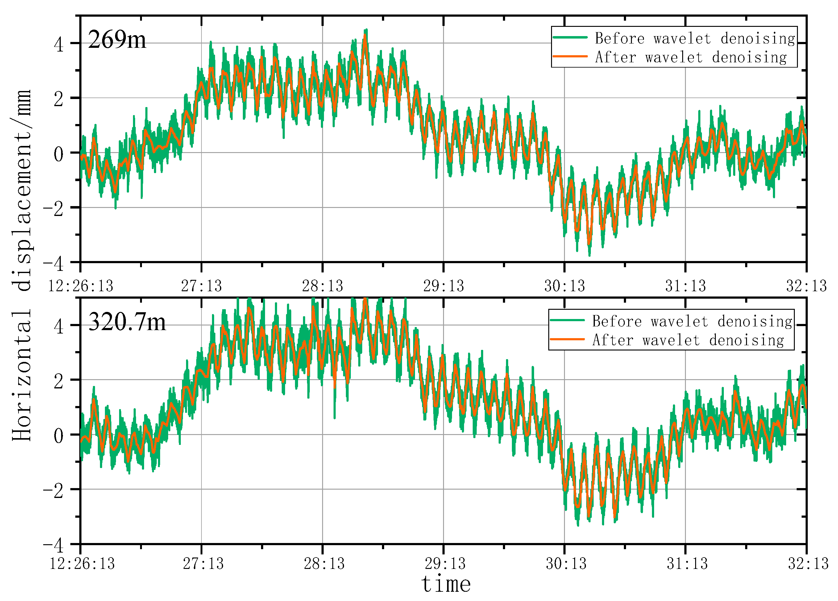
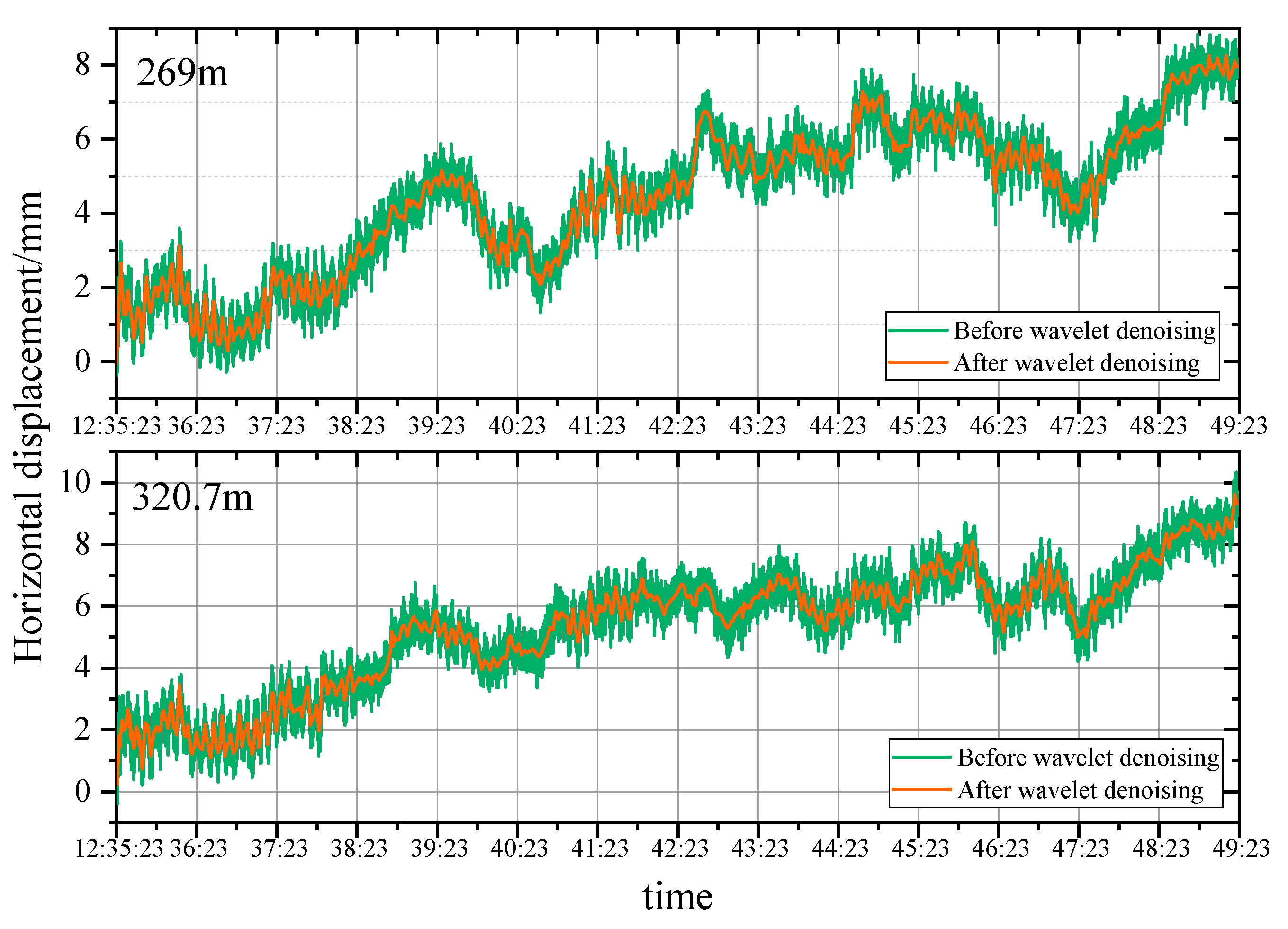
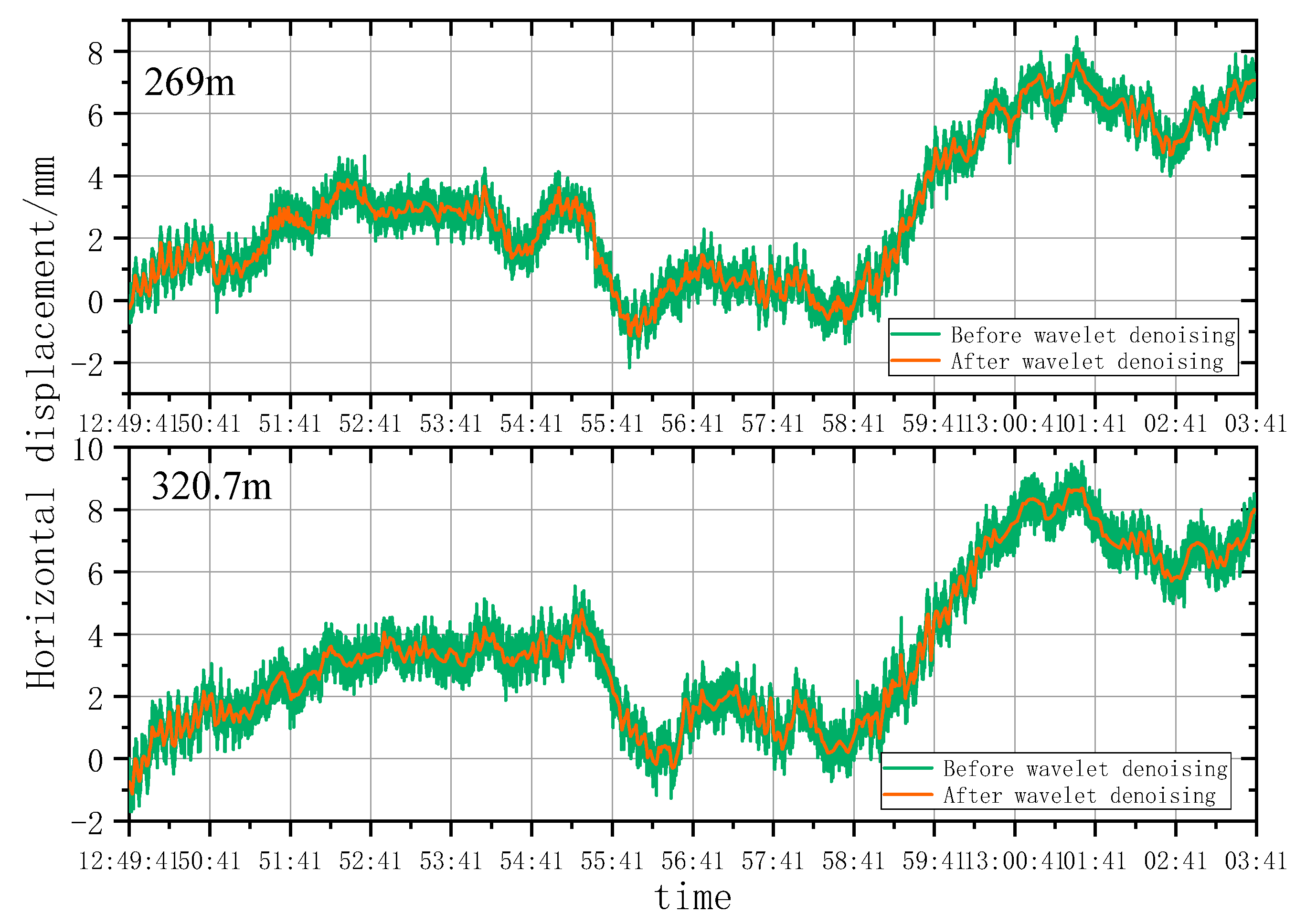
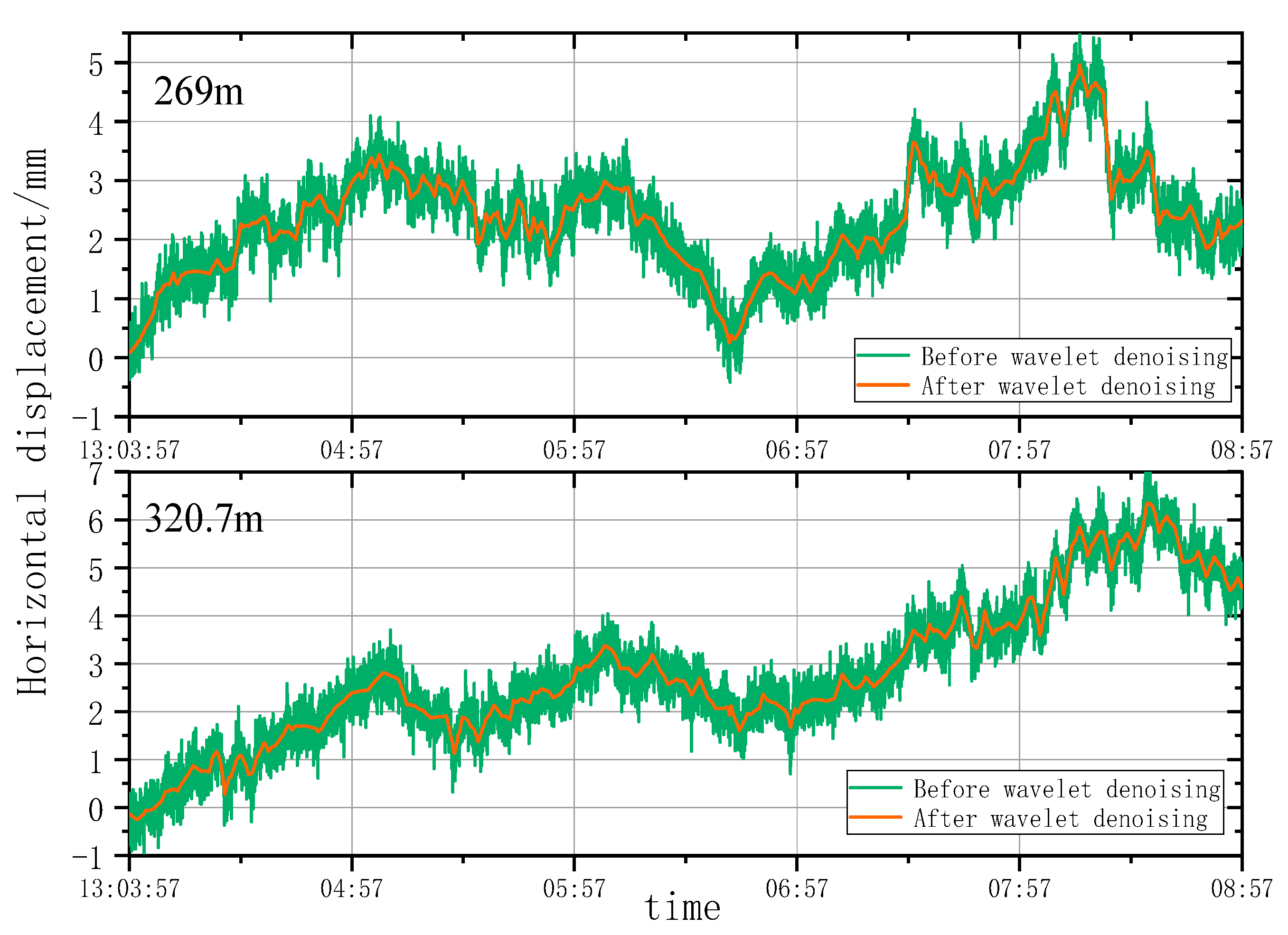
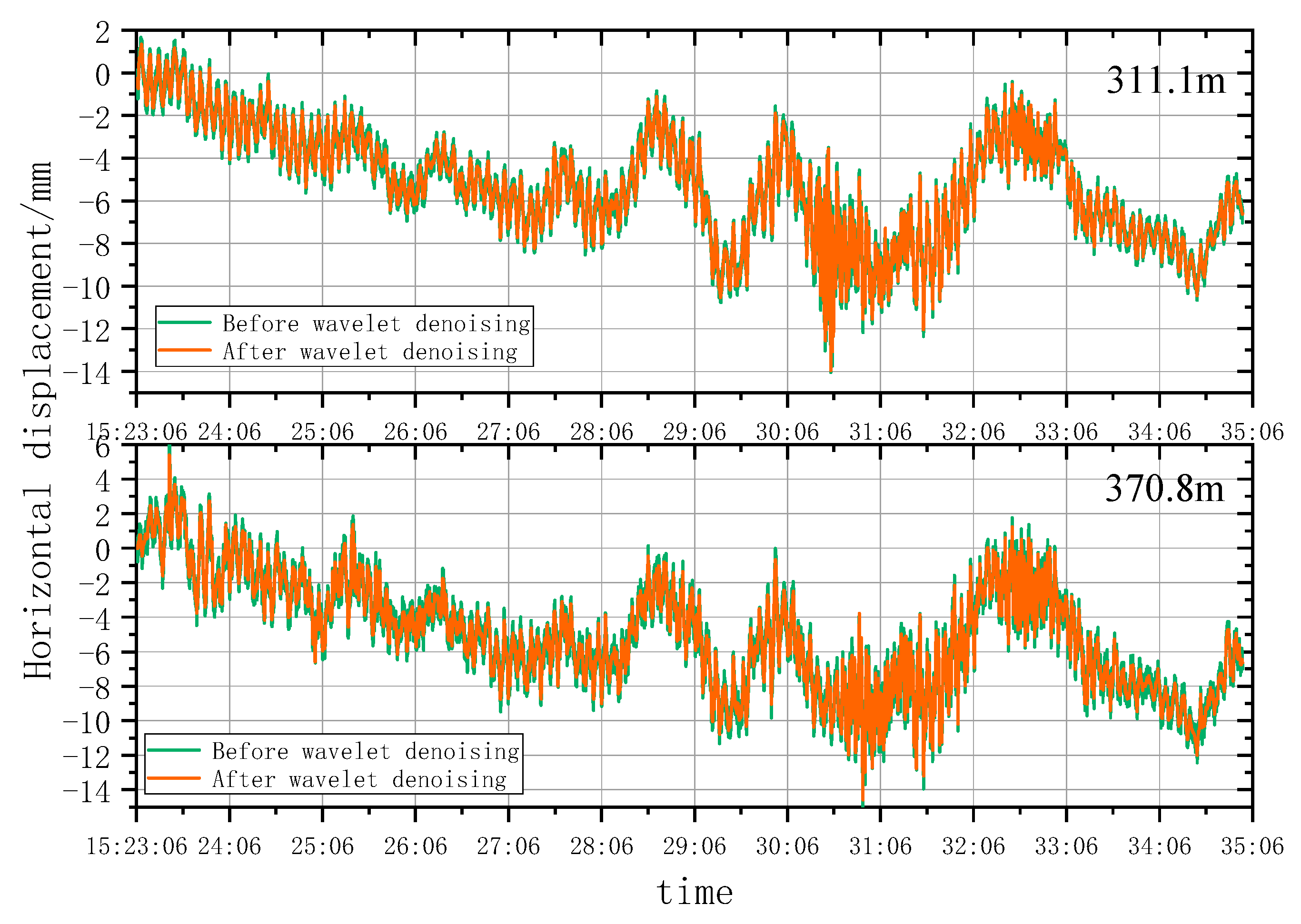
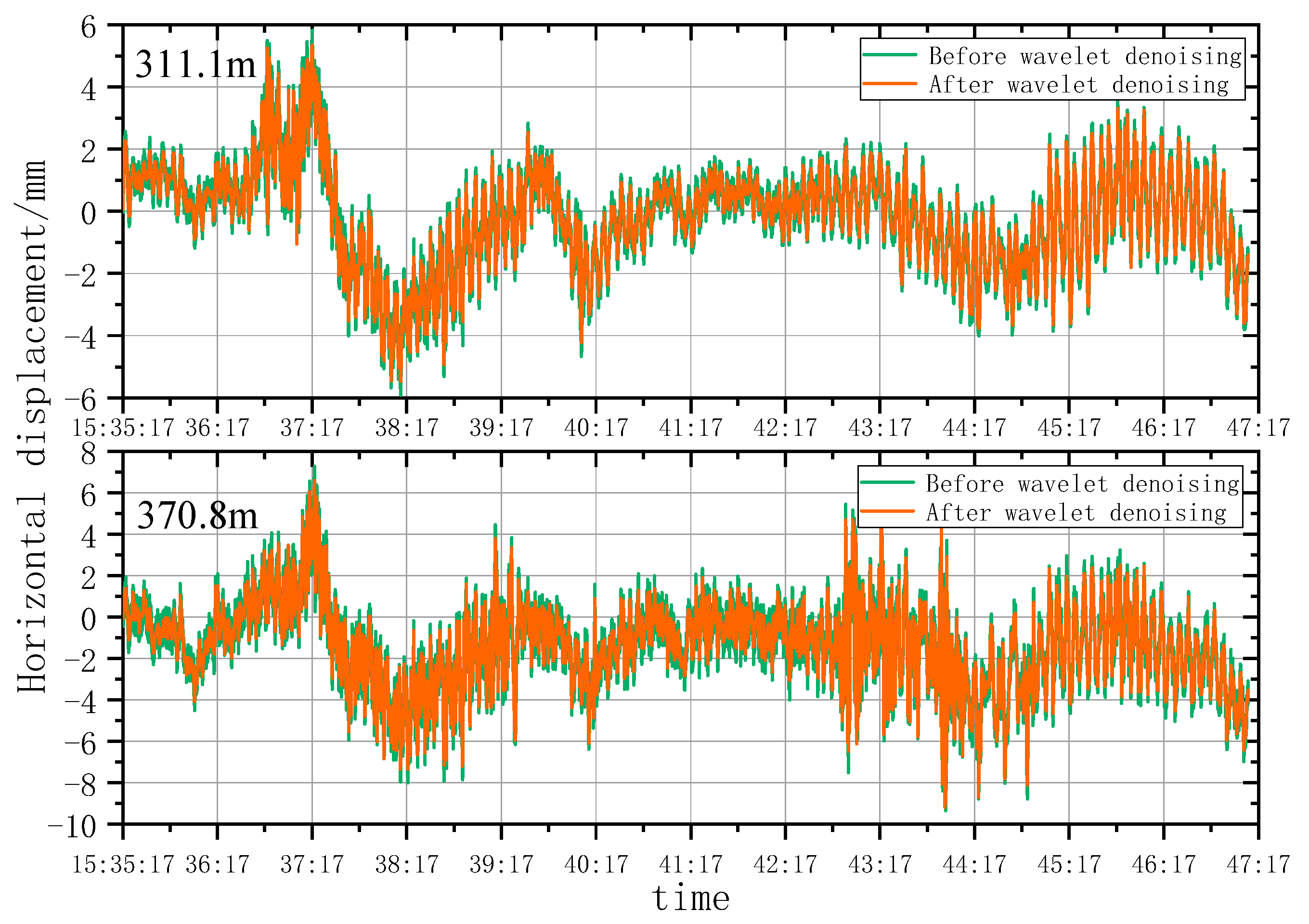
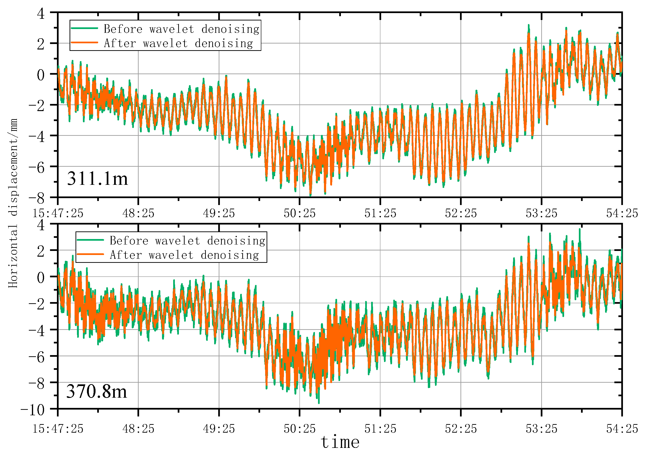
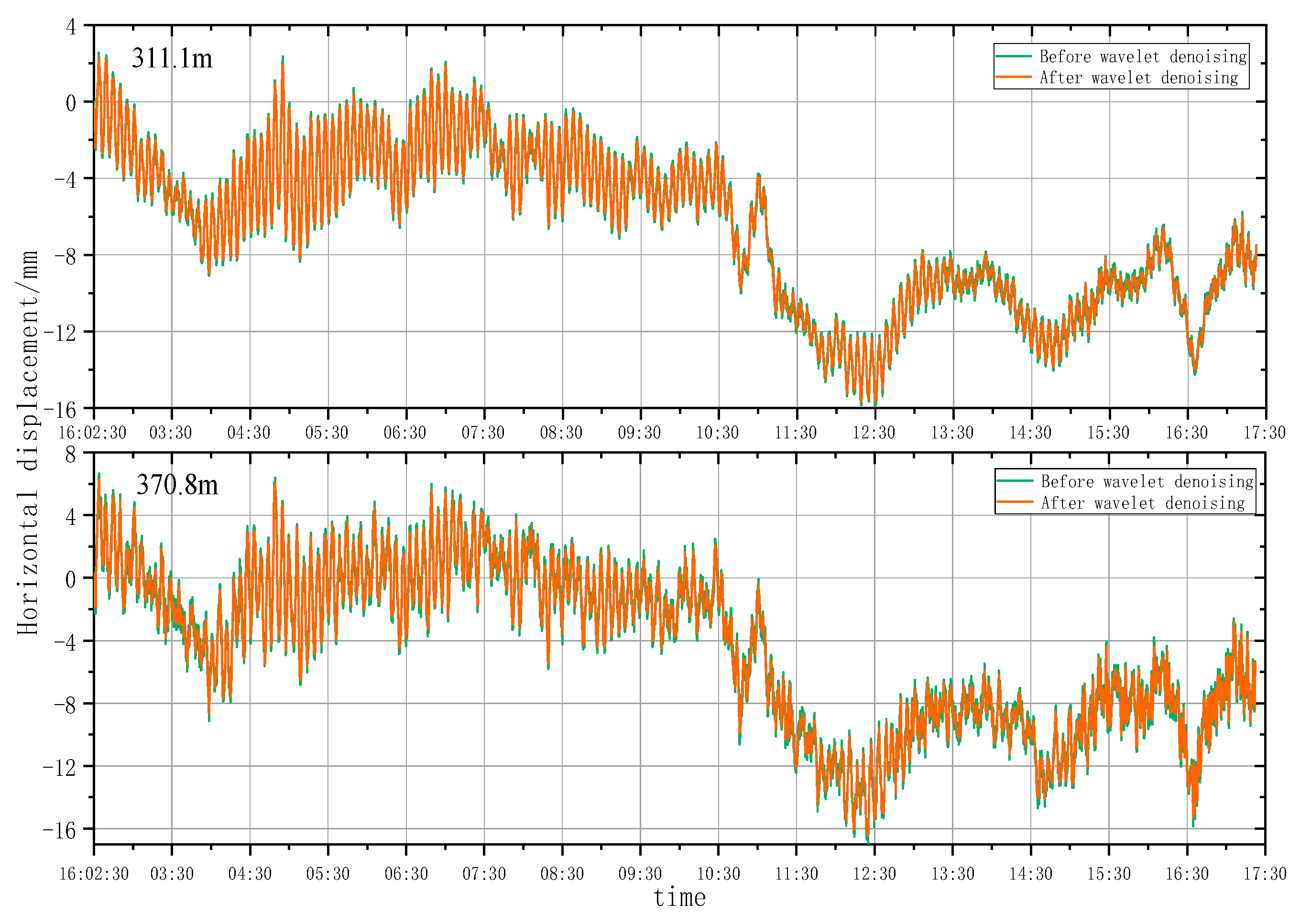
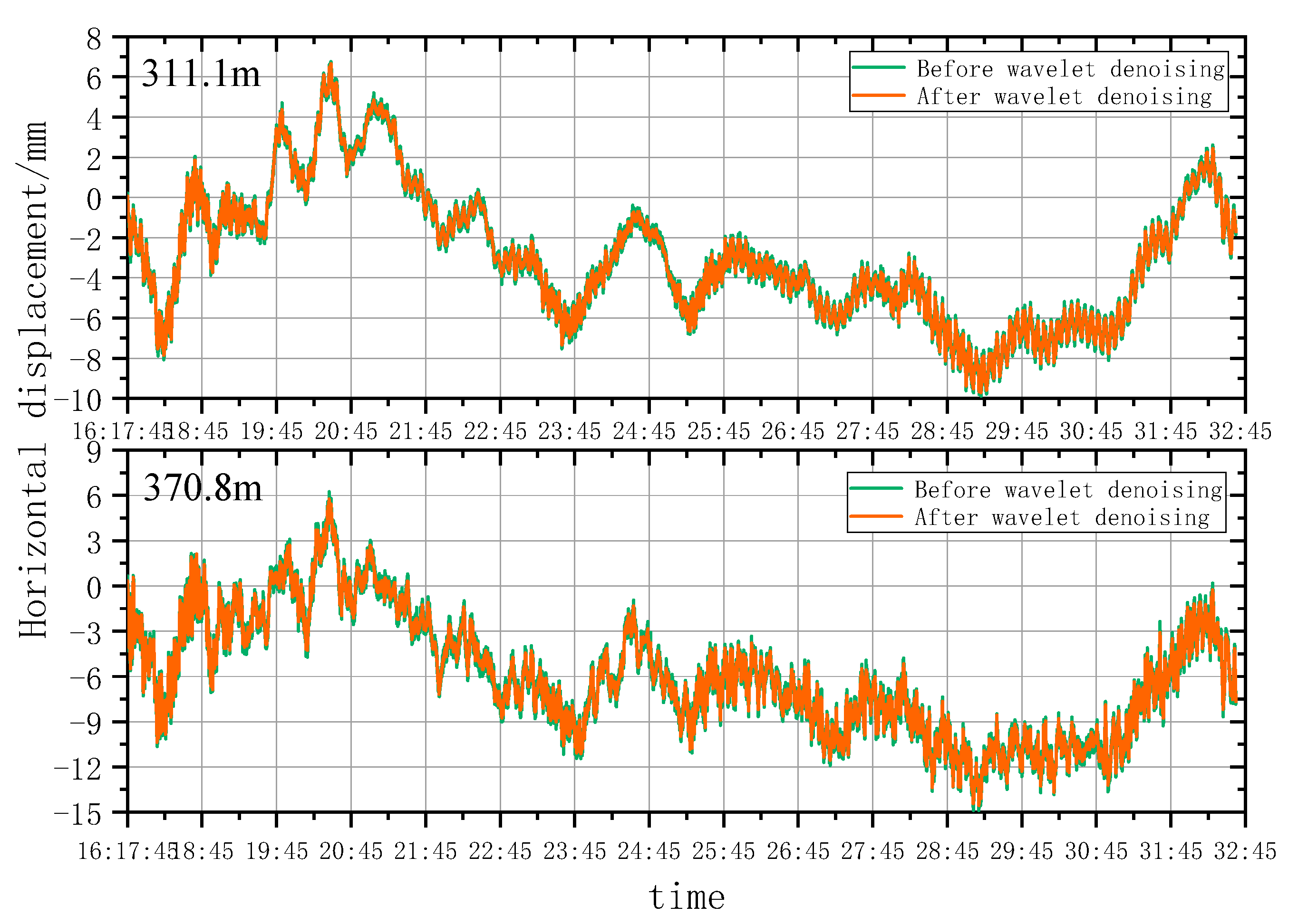
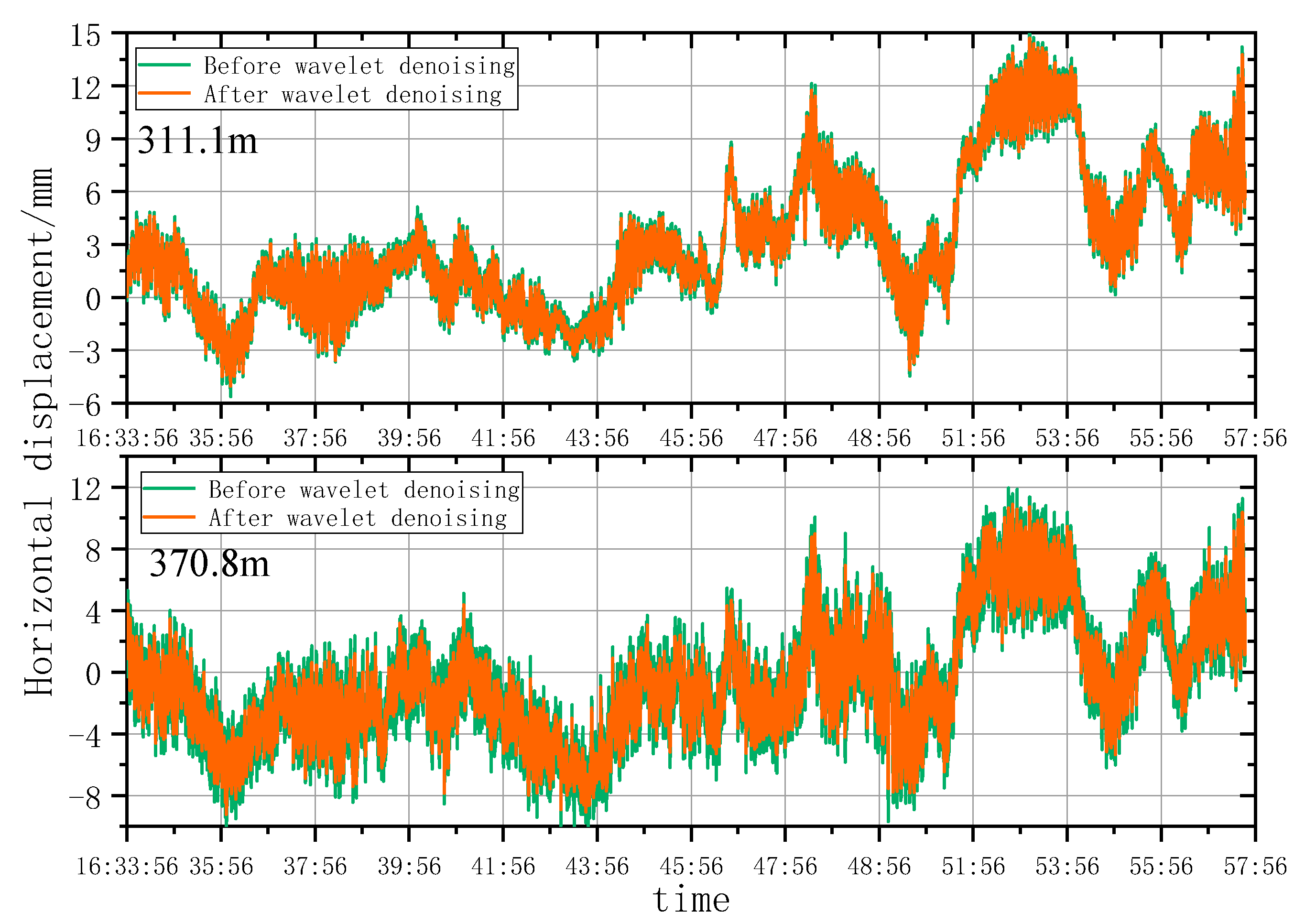
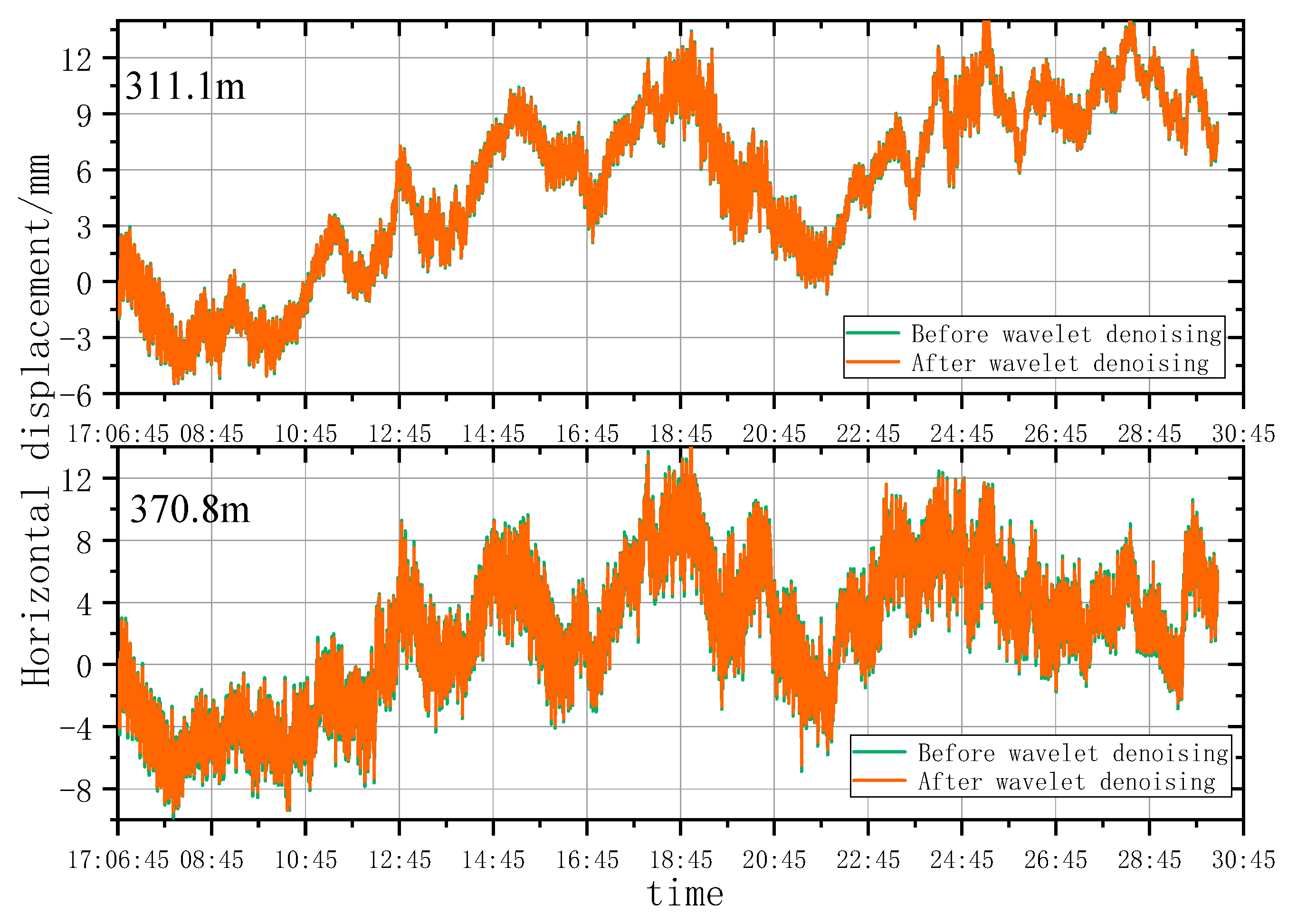
5.1.2. Analysis of Wavelet Denoising Results

In this work, the wavelet denoising effect was characterized by the smoothness index, RMSE, and SSD of the horizontal displacement time series before and after wavelet denoising. The acquired results are presented in

Table 3. Smoothness index, RMSE and sample standard deviation of the horizontal displacement time series.

Yunding Building				Main Tower
Segment of Survey	r (Smoothness Index)	RMSE	SSD	Segment of Survey	r (Smoothness Index)	RMSE	SSD
1106571	0.00925	0.14012	0.75441	1547251	0.00782	0.14943	2.24509
1106572	0.00741	0.14121	0.77505	1547252	0.02069	0.25499	2.20841
1112591	0.00576	0.11541	0.67830	1535171	0.15125	0.17335	1.60989
1112592	0.00284	0.11416	0.72075	1535172	0.05515	0.29064	1.99589
1119581	0.00042	0.27306	0.39560	1523061	0.04298	0.16739	2.57050
1119582	0.00041	0.30948	0.47989	1523062	0.01066	0.26937	3.15948
1149161	0.0072	0.11138	1.72893	1706451	0.53105	0.05253	4.58172
1149162	0.00602	0.11251	1.89729	1706452	0.56674	0.15831	4.39969
1201501	0.00646	0.10794	1.71760	1633561	0.03586	0.16844	3.90771
1201502	0.00563	0.11081	1.89620	1633562	0.07	0.487	3.74168
1126081	0.00108	0.27459	0.72590	1617451	0.01061	0.11254	3.27263
1126082	0.00091	0.30371	1.05497	1617452	0.02368	0.18926	3.89401
1226131	0.00276	0.27737	1.49659	1602301	0.01812	0.11284	4.01258
1226132	0.00261	0.3204	1.71434	1602302	0.03153	0.19844	4.99208
1235231	0.00064	0.282	1.93375	1658431	0.05715	0.16601	2.60052
1235232	0.00052	0.31824	1.91998	1658432	0.14003	0.49929	3.24224
average value	0.00375	0.20702	1.24309	average value	0.11083	0.21561	3.27713

. Clearly, the first six digits in the range series represent the beginning time of the measurement. The 7th digit represents the number of the test site. The existence of a smaller smoothness index (r), RMSE, and SSD indicates that the wavelet denoising effect takes place better. It is easy to conclude from the wavelet analysis that r, RMSE, and SSD of the Yunding Building were both smaller than those of the Main Tower. In particular, r of the Yunding Building was two orders of magnitude lower than that of the Main Tower. Hence, we can believe that the wavelet analysis had a good denoising effect under natural conditions.

To intuitively reflect the wavelet denoising effect, deformation curves before and after wavelet denoising of characteristic points of the Yunding Building and Main Tower were plotted, respectively (Figure 5). As can be seen from Figure 5, the horizontal displacement time series curves gained from the original radar data of the Yunding Building greatly fluctuated, accompanied by many burr points. After performing the wavelet denoising analysis, the burrs of the horizontal displacement time series were basically eliminated and the displacement curve became smoother greatly. However, the curves of the Main Tower, after denoising, still exhibited some fluctuations. The degree of such fluctuations increased with the increase in the height of the characteristic point to the ground. Construction and mild vibration of the buildings during the swing in conjunction with the impact of the external environment may affect the radar signals, thus resulting in mild fluctuation of the displacement curves after performing wavelet denoising.

5.2. Motion State Analysis of the Yunding Building under Natural Conditions

The SNR distribution of the Yunding Building is presented in Figure 6. The SNR of the radar was higher than 30 db within the height range of 200~350 m, indicating that the data collected by radar had good quality. For a better expression of the internal correlation between the deformation of super high-rise buildings and time series, the characteristic points at 269 m and 320.7 m (Points A and B) were chosen to characterize the dynamic deformation characteristics of the Yunding Building. The motion direction far away from the monitoring points of the Yunding Building was recorded as the positive direction, and the opposite was the negative direction.

As can be seen from Figure 7, the horizontal displacement trends at Points A and B from 11:06:57 to 11:11:57 were relatively consistent. The horizontal displacements moved first toward the negative direction and reached the maximum (0.93 mm) at about 11:09. Subsequently, they began to move toward the positive direction and reached the maximum (2.45 mm) at about 11:11. The points of the maximum displacements at the two directions were both at the height of 320.7 m of the building.

As can be observed from Figure 8, the horizontal displacements at Points A and B from 11:12:59 to 11:16:58 fluctuated within −2 to 2 mm. The maximum negative displacement (1.72 mm) occurred at the height of 269 m of the building at about 11:14. On top of that, the maximum positive displacement (1.89 mm) occurred at the height of 320.7 m of the building at about 11:17:50.

According to the reported data in Figure 9, the horizontal displacement at Point A fluctuated around −1~2 mm from 11:12:59 to 11:16:59. Subsequently, it began to move along the negative direction, and the maximum displacement (1.81 mm) was observed at about 11:30. An obvious motion trend similar to a sine curve was detected at the Point B, where the maximum positive displacement (4.14 mm) was reached at 11:28 and maximum negative displacement (0.77 mm) at about 11:30.

In Figure 10, the manifestation of a consistent displacement trend at the two characteristic points from 11:49:16 to 11:59:16 can be detected. The first five minutes were the positive displacement stage, and the maximum displacement (3.83 mm) was reached at about 11:53:46. One minute later, it suddenly changed to move toward the negative direction, and the displacement amplitude was about 6 mm. The maximum negative displacement was reached (5.2 mm). Subsequently, two characteristic points oscillated around the scale line of −2 mm.

As can be ascertained from Figure 11, the displacement trends at two characteristic points from 12:01:50 to 12:09:50 were consistent. The first negative displacement peak took place at about 12:03:50, and then it entered into the positive displacement stage. The maximum positive displacement (0.75 mm) in this test period took place at about 12:04:50. Later, it moved toward the negative direction at a speed of about 2 mm/min, and the maximum negative displacement (7.68 mm) took place at about 12:06:50.

In Figure 12, motion trends similar to the sine curve were observed at two characteristic points from 12:26:13 to 12:32:13. In this period, the maximum positive and negative displacements were taken place at about 12:28:30 and 12:30:30, which were valued at 5.10 mm and 3.33 mm, respectively. The points with maximum displacement were at the height of 320.7 m of the building.

Moreover, in Figure 13, the two characteristic points always presented positive displacement trends at two characteristic points from 12:35:23 to 12:49:23. The maximum displacement was 9.63 mm, and the point with the maximum displacement was at the height of 320.7 m of the building.

According to Figure 14, positive displacement trends at two characteristic points from 12:49:41 to 12:55:41 were observed. At about 12:56:15, there was about 4 mm of negative displacement trend at Point B. Subsequently, it entered into the positive displacement stage again and reached the maximum positive displacement (8.68 mm) at about 13:02:30.

As can be observed in Figure 15, Point A oscillated within 1 to 3 mm from 13:03:57 to 13:06:10, and an about 3 mm negative displacement took place at about 13:06:10. Later, Point A began to move along the positive direction and reached the maximum displacement (4.96 mm) at about 12:08:15. Point B kept moving toward the positive direction from 13:03:57 to 13:08:57, and reached the maximum displacement (6.34 mm) at about 13:08:27.

According to the analysis of horizontal displacement time series at Points A and B, it was found that from 11:6 to 13:03, 25 September 2022, the single-point motion state of the Yunding Building presented the elastic motion state of nonlinear oscillation around the central axis. The maximum oscillation amplitude was 9.63 mm. Additionally, the motion trends of the characteristic points at different heights were consistent most of the time, and obvious differences only occurred at specific moments.

5.3. Motion State Analysis of Main Tower under Natural Conditions

The SNR distribution of the Main Tower is presented in Figure 16. For better expression of the internal correlation between the deformation of the super high-rise building and time series, the characteristic points at 311.1 m and 370.8 m (Points C and D) were chosen to characterize the dynamic deformation characteristics of the Main Tower. The motion direction far away from the monitoring points of the Main Tower was recorded as the positive direction, and the opposite was the negative direction.

According to Figure 17, two characteristic points in the first half period of the monitoring period both moved along with the negative direction and reached the maximum negative displacement (14.58 mm) at about 15:30:36. Subsequently, they oscillated around the scale line of −6 mm.

As can be seen from Figure 18, two characteristic points kept positive displacement in the first two minutes of the monitoring period and reached the maximum positive displacement (6.59 mm) at about 15:37:17. Subsequently, they moved significantly along with the negative direction and the motion amplitude was about 15 mm. The maximum negative displacement reached 9.17 mm at about 15:38:17. In the next 9 min, two characteristic points oscillated within the range of 4 mm~−8 mm.

By considering the reported outcomes in Figure 19, two characteristic points kept moving toward the negative direction in the first-half period of the monitoring. They reached the maximum negative displacement (8.79 mm) at about 15:50:25. Subsequently, two characteristic points moved toward the positive direction at a low speed until the end of monitoring.

According to Figure 20, the displacement trends of two characteristic points were relatively consistent from 16:02:30 to 16:17:30. In the first half period of the monitoring, two characteristic points oscillated within the range of ±4 mm. They kept moving toward the negative direction after 16:10:30 and reached the maximum (16.46 mm) at about 16:12:30. Next, they oscillated within −4 to −16 mm until the end of monitoring.

As can be seen from Figure 21, two characteristic points kept moving toward the positive direction in the first four minutes from 16:17:45 to 16:32:45, and reached the maximum displacement (6.65 mm) at about 16:20:30. Later, they began to move toward the negative direction at the speed of about 6 mm/min until about 16:23:45. In the last 7 min, two characteristic points oscillated within −3 to −15 mm, and the maximum oscillating deformation was 14.57 mm.

In Figure 22, it can be observed that two characteristic points kept moving toward the positive direction in the first half period of the monitoring and reached the maximum positive displacement at 16:45:15. Subsequently, they moved toward the negative by about 15 mm. They reached the maximum negative displacement (9.21 mm) at about 16:50:56. Afterwards, two characteristic points continued to move toward the positive direction by about 20 mm and reached the maximum positive displacement (14.71 mm) at 16:52:56.

In Figure 23, two characteristic points generally kept positive displacement from 17:06:45 to 17:30:45 except in the period from 17:18:45 to 17:21:45. In this monitoring period, the maximum positive displacement and the maximum negative displacement of two characteristic points were 14.47 mm and 9.50 mm, respectively.

According to the analysis of the horizontal displacement time series of Points C and D, the motion states of characteristic points of the Main Tower from 15:23 to 17:06, 25 September 2022, were consistent with those of the Yunding Building. The maximum displacement of the Main Tower was increased to some extent compared to that of the Yunding Building, reaching 16.46 mm.

From the above content, the motion state of super-tall buildings in the natural state presents a nonlinear swaying elastic motion state around the central axis. If other conditions remain unchanged, construction factors will have a certain impact on the swing amplitude.

6. Dynamic Analysis of Super-Tall Buildings under Wind Load

6.1. Motion State Analysis of the Yunding Building under Wind Loads

In the monitoring period, the external wind loads suddenly increased from 9:56 to 10:30 on 25 September 2022. Thus, the super high-rise buildings developed significant oscillation deformation. According to deformation monitoring data, the displacement curves of characteristic points with time series (Figure 24).

As can be seen from Figure 24, the displacement curves of characteristic points at 200.5 m, 230 m, 266.6 m, and 316.7 m basically oscillated around a scale line in periods of 9:56:01~10:10:01, 10:10:17~10:24:14, and 10:10:17~10:24:14.

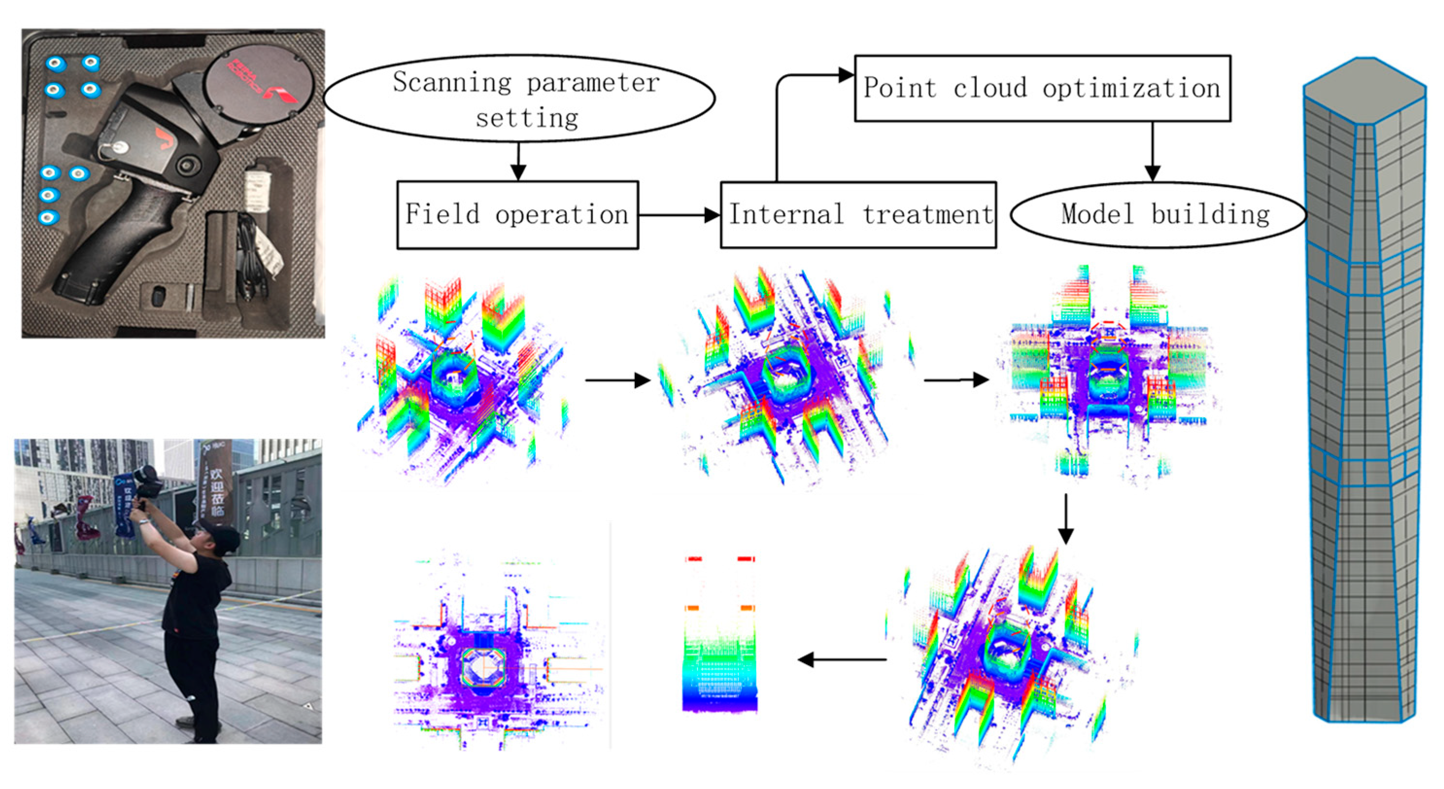
6.2. State Visualization of Genting Building under Wind Load Based on LiDAR Technology

In order to visually display the movement of the Yunding Building under wind load, we used a handheld LiDAR scanner to collect data within 100 m of the building during field operations, and then used the SLAM GO POST module of the software drone manager to process point cloud data and obtain panoramic images to obtain the main parameters of the LiDAR scanner as shown in

Table 4. Main parameters of LiDAR scanner.

Laser Field Angle	Camera Field Angle	Relative Accuracy/Precision	Number of Laser Channels	Maximum Ranging	Dot Frequency	Echo Intensity	Number of Cameras	Camera Resolution
270° × 360°	200° × 100°	2 cm/5 cm	16	100 m	300 kpts/s	8 bits	3	500,000,000

. Finally, we modelled the results using revit.

Firstly, the data information within 100 m of the Genting building was collected by using Pegasus SLAM100 handheld LiDAR scanner in field operations, and then the SLAM GO POST module in the software drone manager was used for point cloud data processing and panoramic image acquisition. The brief operation steps are as follows: a new project, a one-click data solution to obtain the original point cloud, then point cloud color, the image color of the point cloud data, and finally, point cloud optimization. After performing this step, the software will optimize the original point cloud, denoise and other processing, which can make the point cloud effect more uniform and delicate. In this way, point clouds in the southeast, northeast, southwest, and due south of the Genting Building are obtained. Finally, point cloud cutting is performed to obtain a single point cloud of the Genting Building, as shown in Figure 25.

According to the obtained point cloud information of Genting Building, the building model of Genting Building is constructed by inserting the cloud function into Revit software. The modeling process is as follows:

(1)

Open the revit software, enter the interface, select a new volume in the panel, and click to enter.

(2)

After entering, according to the point cloud information of the Genting building, use the insertion cloud command and the line command to draw, paying special attention to the check of the 3D capture command.

(3)

Load the drawn model into the building template and modify the appearance of the volume. In this step, considering that the overall building structure of the Genting building tends to be integrated and similar, the modeling process can build the overall 339 m height building model through the principle of mirror symmetry according to the obtained point cloud information within 100 m of the height of the Genting building. Since the purpose of our modeling is to simulate the motion state of the building under wind load rather than the building itself, there are no special strict requirements for the width of the building during the modeling process.

(4)

Click volume and site, select wall, and add wall to volume model.

(5)

Click volume and site again. Select a curtain wall system and add a glass curtain wall to the volume model. The curtain wall network can be customized.

(6)

Use the type attribute to change the color of the window wall to silver gray in order to simulate the solid color of the Genting building and achieve a beautiful model. By combining the obtained model with Figure 24 in the previous section, it is found that the motion state of super-tall buildings under wind load mainly switches back and forth between the S-shape, hyperbolic line and oblique line, and has obvious elastic deformation characteristics.

As can be ascertained from Figure 26, the displacement curves were marked in green, yellow, and red according to the increasing order of the time series. It can also be seen from Figure 26a that the Yunding Building oscillated within −300.99 mm to 738.52 mm from 9:56:01 to 10:10:01. The overall motion state changed from a straight line to an S-shaped pattern and finally evolved into hyperbolic type.

As can be seen from Figure 26b, the Yunding Building oscillated within −633.09 mm to 854.21 mm from 10:10:17 to 10:24:14. The overall motion state changed from a hyperbolic type to an S-shaped pattern gradually.

What’s more, as can be seen from Figure 26c, the Yunding Building oscillated within −398.55 mm to 895.79 mm from 10:24:33 to 10:29:33. The overall motion state changed from an S-shaped pattern to the hyperbolic type gradually.

7. Conclusions

In this work, dynamic deformation information of the Jinan Yunding Building and the Main Tower of Shandong International Financial Center was acquired by using the GB-RAR technology. Meanwhile, the accuracy of the collected deformation information was improved through wavelet denoising. The following major conclusions could be drawn:

(1)

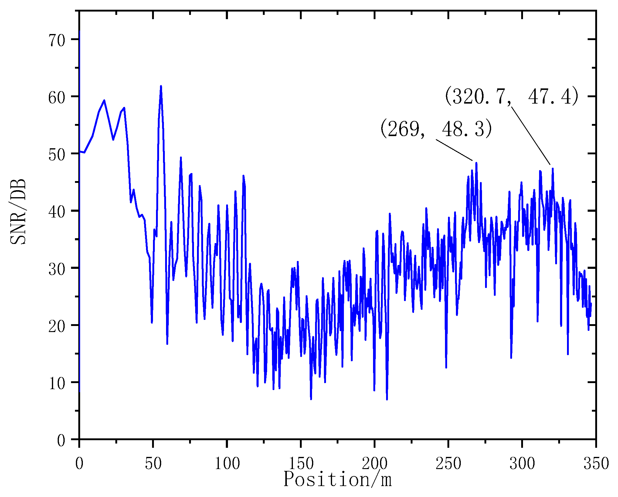
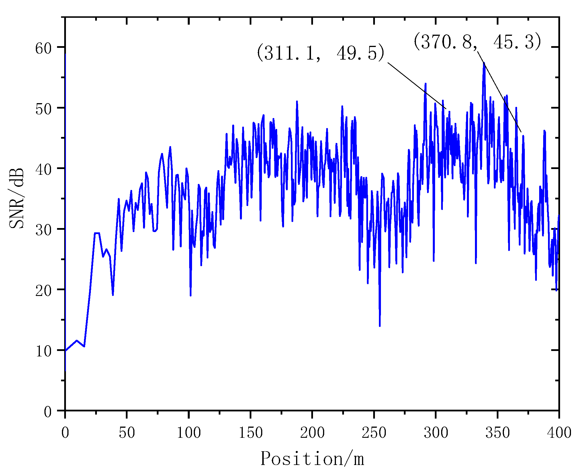
Yunding Building is located in CBD, surrounded by high-rise buildings. The SNR of the radar in the height range of 200 m~350 m to the ground was higher than 30 db. The data collected by radar had good quality. The Main Tower of Shandong International Financial Center was surrounded by no high-rise buildings and had a small influence on radar signals. The SNR of radar above 50 m from the ground was higher than 30 db and the data collected by radar exhibited good quality.

(2)

According to the smoothness index and RMSE analysis, the wavelet analysis can effectively eliminate noises under natural conditions and remove burrs in the time series deformation curves of horizontal displacement significantly. However, the wavelet denoising effect is highly sensitive to construction factors when the architect is under construction. As a result, the time series deformation curves of horizontal displacement after denoising still had serious burrs.

(3)

The single-point motion state of super high-rise buildings presents an elastic motion state of nonlinear oscillation around the central axis. Motion states of the characteristic points at different heights generally had consistent trends at most moments, and obvious differences only occurred at specific moments. Under natural conditions, the maximum oscillation amplitude of the Yunding Building and the Main Tower was 9.63 mm and 16.55 mm, respectively.

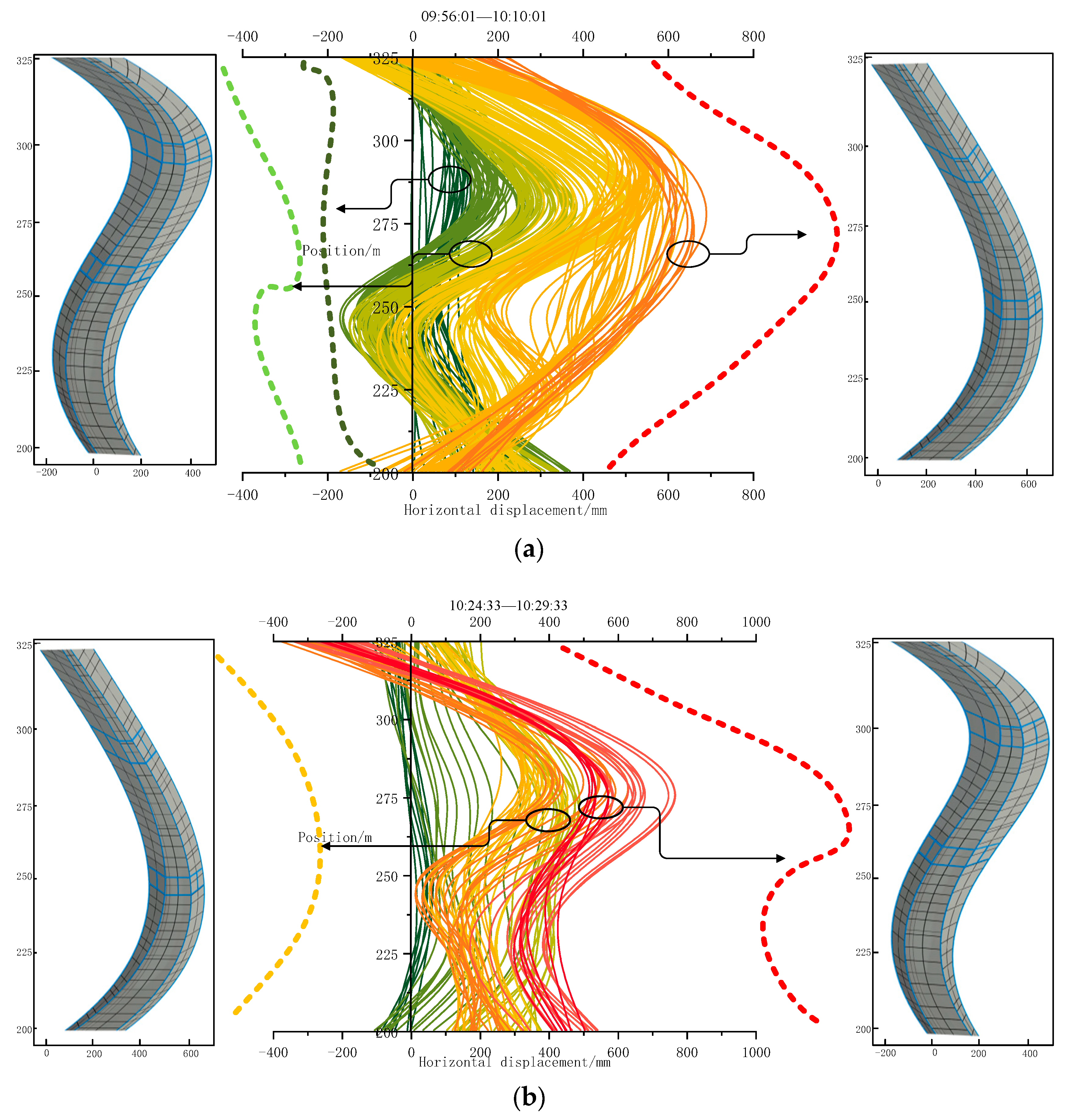
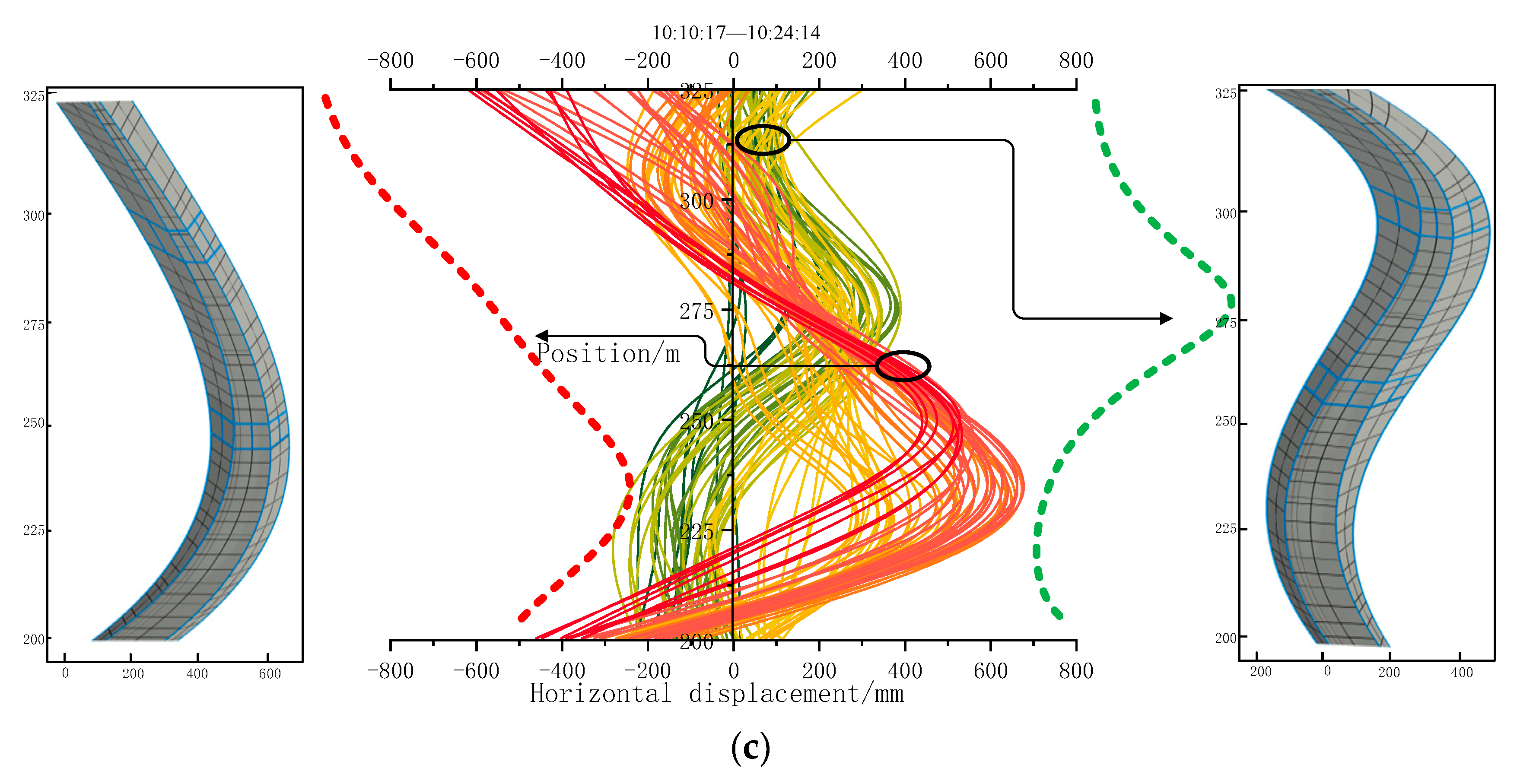
(4)

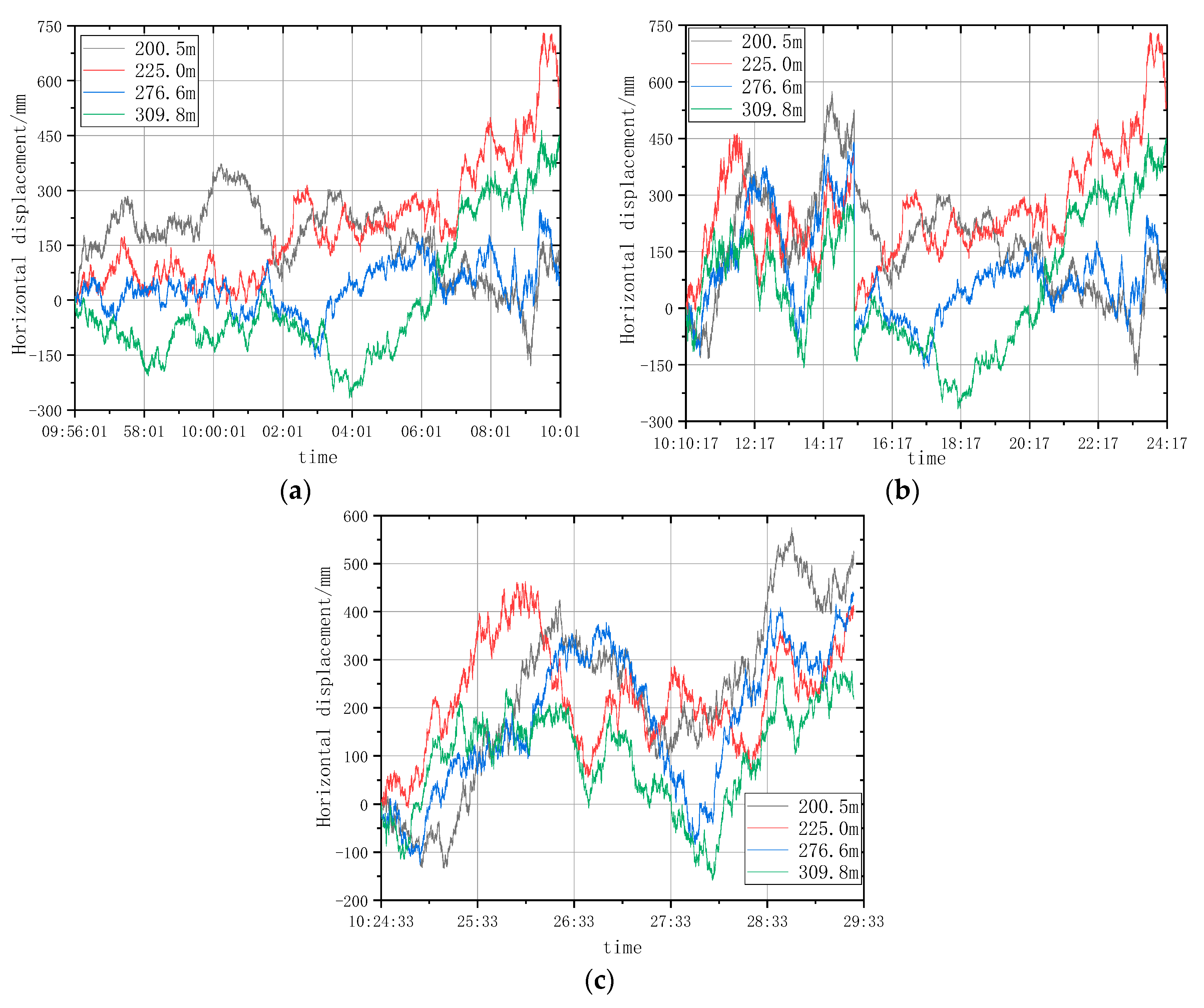
The external wind loads suddenly increased from 9:56 to 10:30 on 25 September 2022. According to deformation monitoring data, the Yunding Building oscillated within −300.99 mm to 738.52 mm from 9:56:01 to 10:10:01. The Yunding Building oscillated within −633.09 mm to 854.21 mm from 10:10:17 to 10:24:14 and within −398.55 mm to 895.79 mm from 10:24:33 to 10:29:33.

(5)

The three-dimensional visualization model of the Genting Building was established based on handheld LiDAR technology, and the spatial state of the super tall building under wind load was obtained through simplified processing by revit, showing the characteristics of switching back and forth between an S-shape, hyperbolic line and oblique line and nonlinear elastic deformation.

References

1. Ji, S.; Liu, S.; Li, Y. Response characteristics of super high-rise building subjected to far-field long-period ground motion. J. Build. Struct. 2018, 11, 1–10. [Google Scholar]
2. Fuyuki, A.; Kohei, F.; Masaaki, T.; Izuru, T. Importance of interstory velocity on optimal along-height allocation of viscous oil dampers in super high-rise buildings. Eng. Struct. 2013, 56, 489–500. [Google Scholar]
3. Li, Q.; He, Y.; He, Y.; Zhou, K.; Han, X. Monitoring wind effects of a landfall typhoon on a 600 m high skyscraper. Struct. Infrastruct. Eng. 2019, 15, 54–71. [Google Scholar] [CrossRef]
4. Silva, I.D.; Ibañez, W.; Poleszuk, G. Experience of Using Total Station and GNSS Technologies for Tall Building Construction Monitoring. In Proceedings of the International Congress and Exhibition Sustainable Civil Infrastructures: Innovative Infrastructure Geotechnology, Sharm El Sheikh, Egypt, 15–19 July 2017. [Google Scholar]
5. Xu, J.; Jo, H. Development of High-Sensitivity and Low-Cost Electroluminescent Strain Sensor for Structural Health Monitoring. IEEE Sens. J. 2016, 16, 1962–1968. [Google Scholar]
6. Li, Q.; Xiao, Y.; Wong, C. Full-scale monitoring of typhoon effects on super tall buildings. J. Fluids Struct. 2005, 20, 297–717. [Google Scholar] [CrossRef] [Green Version]
7. Xia, Y.; Zhang, P.; Ni, Y.; Zhu, H. Deformation monitoring of a super-tall structure using real-time strain data. Eng. Struct. 2014, 67, 29–38. [Google Scholar] [CrossRef] [Green Version]
8. Wang, T.; Xu, Y. Research on Dynamic Characteristic Monitoring Methods for Super High-rise Building. Bull. Surv. Mapp. 2017, 4, 89–92. [Google Scholar]
9. Zhang, X.; Zhang, Y.; Li, B.; Qiu, G. GNSS-Based Verticality Monitoring of Super-Tall Buildings. Appl. Sci. 2018, 8, 991. [Google Scholar] [CrossRef] [Green Version]
10. Li, Q.; Zhi, L.; Yi, J.; To, A.; Xie, J. Monitoring of typhoon effects on a super-tall building in Hong Kong. Struct. Control Health Monit. 2014, 21, 926–949. [Google Scholar] [CrossRef]
11. Li, Q.; Yi, J. Monitoring of dynamic behaviour of super-tall buildings during typhoons. Struct. Infrastruct. Eng. 2016, 12, 289–311. [Google Scholar] [CrossRef]
12. Hwang, J.; Yun, H.; Park, S.; Lee, S. Optimal methods of RTK-GPS/accelerometer integration to monitor the displacement of structures. Sensors 2012, 12, 1014–1034. [Google Scholar] [CrossRef] [Green Version]
13. Fabio, C.; Clemente, F. Monitoring a steel building using GPS sensors. Smart Struct. Syst. 2011, 7, 349–363. [Google Scholar]
14. Guo, Y.; Kareem, A.; Ni, Y.; Liao, W. Performance evaluation of Canton Tower under winds based on full-scale data. J. Wind Eng. Ind. Aerodyn. 2012, 104, 116–128. [Google Scholar]
15. Xiong, C.; Niu, Y. Investigation of the Dynamic Behavior of a Super High-rise Structure using RTK-GNSS Technique. KSCE J. Civ. Eng. 2019, 23, 654–665. [Google Scholar]
16. Gao, Y.; Dian, Z.; Zhang, S.; Zhang, Y.; Li, S. Adaptive local gradient estimation smoothing UKF phase unwrapping algorithm. J. China Univ. Min. Technol. 2022, 51, 1007–1015. [Google Scholar]
17. Li, R.; Chang, L.; Qin, H. Application of InSAR Technology in Deformation Monitoring of Super High Rise Buildings. Constr. Qual. 2021, 39, 70–73. [Google Scholar]
18. Wu, W.; Cui, H.; Hu, J.; Yao, L. Detection and 3D Visualization of Deformations for High-Rise Buildings in Shenzhen, China from High-Resolution TerraSAR-X Datasets. Appl. Sci. 2019, 9, 3818. [Google Scholar]
19. Zhou, L. Monitoring and Analysis of Surface Subsidence and Building Deformation by Radar Interferometry. Ph.D. Thesis, Wuhan University, Wuhan, China, June 2018. [Google Scholar]
20. Tapete, D.; Casagli, N.; Luzi, G.; Fanti, R.; Gigli, G.; Leva, D. Integrating radar and laser-based remote sensing techniques for monitoring structural deformation of archaeological monuments. J. Archaeol. Sci. 2013, 40, 176–189. [Google Scholar] [CrossRef] [Green Version]
21. Marchisio, M.; Piroddi, L.; Ranieri, G.; Calcina, S.V.; Farina, P. Comparison of natural and artificial forcing to study the dynamic behaviour of bell towers in low wind context by means of ground-based radar interferometry: The case of the Leaning Tower in Pisa. J. Geophys. Eng. 2014, 11, 055004. [Google Scholar] [CrossRef]
22. Luzi, G.; Monserrat, O.; Crosetto, M. The Potential of Coherent Radar to Support the Monitoring of the Health State of Buildings. Res. Nondestruct. Eval. 2012, 23, 125–145. [Google Scholar]
23. Zhou, L.; Guo, J.; Wen, X.; Ma, J.; Yang, F.; Wang, C.; Zhang, D. Monitoring and Analysis of Dynamic Characteristics of Super High-rise Buildings using GB-RAR: A Case Study of the WGC under Construction, China. Appl. Sci. 2020, 10, 808. [Google Scholar] [CrossRef] [Green Version]
24. Montuori, A.; Luzi, G.; Bignami, C.; Gaudiosi, I.; Stramondo, S.; Crosetto, M.; Buongiorno, M.F. The Interferometric Use of Radar Sensors for the Urban Monitoring of Structural Vibrations and Surface Displacements. IEEE J. Sel. Top. Appl. Earth Obs. Remote Sens. 2016, 9, 3761–3776. [Google Scholar] [CrossRef]
25. Cheng, Y.; Wu, Z.; Zhou, Y. Three-dimensional Reconstruction of Soviet-style Courtyard Based on Terrestrial LiDAR. Mod. Surv. Mapp. 2021, 5, 50–54. [Google Scholar]
26. Zhou, J.; Tian, J.; Chen, Y.; Mao, Q.; Li, Q. Research on Data Fusion Method of Ground-Based SAR and 3D Lase Scanning. J. Geomat. 2015, 3, 26–30. [Google Scholar]
Figure 1. Relationship between the visual and horizontal displacements.
Remotesensing 15 03651 g001
Figure 2. IBIS system accuracy verification experiment: (a) IBIS system and TCA2003; (b) front-end reflector; (c) test site.
Remotesensing 15 03651 g002
Figure 3. Deformation monitoring diagram of the Yunding Building. (a) Ground view of the Yunding Building from the location of the IBIS-S system; (b) View of the IBIS system on S1.
Remotesensing 15 03651 g003
Figure 4. Deformation monitoring diagram of Main Tower. (a) Ground view of Main Tower from the location of the IBIS system; (b) View of the IBIS-S system on S2.
Remotesensing 15 03651 g004
Figure 5. Comparison of the wavelet denoising effects.
Remotesensing 15 03651 g005
Figure 6. SNR distribution of the Yunding Building.
Remotesensing 15 03651 g006
Figure 7. Horizontal displacements at characteristic points of the super high−rise building from 11:06:57 to 11:11:57.
Remotesensing 15 03651 g007
Figure 8. Horizontal displacements at characteristic points of the super high-rise building from 11:12:59 to 11:16:59.
Remotesensing 15 03651 g008
Figure 9. Horizontal displacements at characteristic points of the super high-rise building from 11:26:08 to 11:31:08.
Remotesensing 15 03651 g009
Figure 10. Horizontal displacements at characteristic points of the super high-rise building from 11:49:16 to 11:59:16.
Remotesensing 15 03651 g010
Figure 11. Horizontal displacements at characteristic points of the super high-rise building from 12:01:50 to 12:09:50.
Remotesensing 15 03651 g011
Figure 12. Horizontal displacements at characteristic points of the super high-rise building from 12:26:13 to 12:32:13.
Remotesensing 15 03651 g012
Figure 13. Horizontal displacements at characteristic points of the super high-rise building from 12:35:23 to 12:49:23.
Remotesensing 15 03651 g013
Figure 14. Horizontal displacements at characteristic points of the super high-rise building from 12:49:41 to 13:03:41.
Remotesensing 15 03651 g014
Figure 15. Horizontal displacements at characteristic points of the super high-rise building from 13:03:57 to 13:08:57.
Remotesensing 15 03651 g015
Figure 16. SNR distribution of the Main Tower.
Remotesensing 15 03651 g016
Figure 17. Horizontal displacement sequences of characteristic points from 15:23:06 to 15:35:06.
Remotesensing 15 03651 g017
Figure 18. Horizontal displacement sequences of characteristic points from 15:35:17 to 15:47:17.
Remotesensing 15 03651 g018
Figure 19. Horizontal displacement sequences of characteristic points from 15:47:25 to 15:54:25.
Remotesensing 15 03651 g019
Figure 20. Horizontal displacement sequences of characteristic points from 16:02:30 to 16:17:30.
Remotesensing 15 03651 g020
Figure 21. Horizontal displacement sequences of characteristic points from 16:17:45 to 16:32:45.
Remotesensing 15 03651 g021
Figure 22. Horizontal displacement sequences of characteristic points from 16:33:56 to 16:57:56.
Remotesensing 15 03651 g022
Figure 23. Horizontal displacement sequences of characteristic points from 17:06:45 to 17:30:45.
Remotesensing 15 03651 g023
Figure 24. Motion states of characteristic points of the Yunding Building under wind loads, (a) 9:56:01~10:10:01, (b) 10:10:17~10:24:14, (c) 10:10:17~10:24:14.
Remotesensing 15 03651 g024
Figure 25. Data processing flow of the point cloud.
Remotesensing 15 03651 g025
Figure 26. Overall motion states of the Yunding Building under wind loads. In order to make it easier to observe, we separately draw the movement curve of Yunding Building at a certain time with dotted lines to compare with the models on both sides. (a) 9:56:01~10:10:01; (b) 10:10:17~10:24:14;(c) 10:10:17~10:24:14.
Remotesensing 15 03651 g026aRemotesensing 15 03651 g026b