Article

Simulation of Land Use Based on Multiple Models in the Western Sichuan Plateau

1
Key Evaluation and Monitoring in Southwest China, Ministry of Education, Sichuan Normal University, Chengdu 610066, China
2
The Faculty of Geography and Resources Sciences, Sichuan Normal University, Chengdu 610101, China
3
Department of Geosciences and Natural Resource Management, University of Copenhagen, 1350 Copenhagen, Denmark
4
Department of Earth System Science, Ministry of Education Key Laboratory for Earth System Modeling, Institute for Global Change Studies, Tsinghua University, Beijing 100084, China
*
Author to whom correspondence should be addressed.
Remote Sens. 2023, 15(14), 3629; https://doi.org/10.3390/rs15143629
Submission received: 26 June 2023 / Revised: 15 July 2023 / Accepted: 19 July 2023 / Published: 21 July 2023

Abstract

:
Many single-land-use simulation models are available to simulate and predict Land Use and Land Cover Change (LUCC). However, few studies have used multiple models to simulate LUCC in the same region. The paper utilizes the CA-Markov model, Land Change Modeler (LCM), and Patch-generating Land Use Simulation model (PLUS) with natural and social driving factors to simulate the LUCC on the Western Sichuan Plateau, using Kappa coefficient, overall accuracy (OA), and Figure of Merit (FoM) to verify the accuracy of the model, and selects a suitable model to predict the LUCC and landscape pattern in the study area from 2020 to 2070. The results are as follows: (1) The LCM has the highest simulation effect, and its Kappa coefficient, OA, and FoM are higher than the other two models. (2) The area of land types other than grassland and wetland will increase from 2020 to 2070. Among them, the grassland area will decrease, but is still most prominent land category in this region. The proportion of wetland areas remains unchanged. The fragmentation degree of forest (F), grassland (GL), shrubland (SL), water bodies (WBs), bare areas (BAs), and permanent ice and snow (PIS) decreases, and the distribution shows a trend of aggregation. The dominance of F and C decreases but still dominates in the landscape. The overall landscape aggregation increased and complexity decreased, and each landscape type’s diversity, evenness, and richness increased, presenting as a more reasonable development. Using multiple models to simulate the LUCC in the same region, and choosing the most suitable local land model is of great significance to scientifically manage and effectively allocate the land resources in the field.

1. Introduction

LUCC is a vital component of research on global environmental changes and sustainable development. It is influenced by natural and human factors, and can be analyzed qualitatively and calculated quantitatively [1,2,3,4]. Scholars at home and abroad have constructed various simulation models for different regions or research needs. These are classified into three categories: quantitative prediction models, spatial prediction models, and coupled models. Quantitative prediction models only analyze changes in land-use quantity and area and are unable to examine the spatial information of LUCC [5,6], including the Markov model, gray model (GM) and system dynamics model (SD) [7,8,9,10]. Spatial prediction models can respond to the spatial information of LUCC and predict its spatial distribution pattern [11], including the cellular automaton model (CA), CLUE-S model, etc. [12,13]. To meet the higher demands of LUCC model research, contemporary LUCC model research has evolved to study multiple coupled models, which combine quantitative and spatial models, including the CA-Markov model, PLUS model, LCM and LandSDS systems [14,15,16,17]. A large number of scholars have demonstrated the feasibility of using coupled models for LUCC studies [18,19].
There are many studies related to simulating and predicting LUCC using a certain model. Still, relatively few studies use multiple models to simulate and predict LUCC in the same region [20]. Simulating LUCC in the same region with multiple simulation models and selecting the most suitable model is necessary for the scientific use of land in this region. Among the many models, the CA-Markov model, LCM, and PLUS model are used worldwide in several fields. These models have received much attention recently and are a hot topic in LUCC research. The three models have various advantages and disadvantages [21,22,23], as well as similarities when using the Markov model to calculate land demand. However, the algorithms involved in these models are different, and the three models have both similarities and differences. Therefore, it is necessary to analyze their similarities and differences in the same region.
The Western Sichuan Plateau is rich in natural landscape elements and serves as a barrier to natural environmental protection [24]. The Western Sichuan Plateau is relatively backward in terms of socioeconomic development and is relatively underdeveloped compared to other regions in China [25]. There is an uncoordinated development between ecological conservation and social economy in this area, and land-planning simultaneously affects local ecological conservation and social-economic development. Scholars have been aware of these problems and used different models to simulate LUCC in the western Sichuan plateau, but there are few research results, single analysis methods and accuracy indicators, and most studies only used a single model, such as the CA-Markov model [25,26]. Based on previous studies, we selected a number of different models to simulate the research area, aiming to find a suitable model for the LUCC simulation of the Western Sichuan Plateau, and to clarify the development trend of LUCC and landscape pattern in the study area to provide data support for the optimal management of land in this region and to realize the harmonious development of the social economy and environmental protection on this basis.
This paper selected the CA-Markov, LCM, and PLUS models to simulate the LUCC in the western Sichuan plateau. The LUCC future development trends were analyzed, aiming to provide a theoretical basis for land management and allocation, realize the adequate configuration of land resources in the study area, and seek harmonious development with the coexistence of the social economy and environmental conservation. The aims of this paper are as follows: (1) explore models suitable for simulating LUCC in the Western Sichuan Plateau, (2) simulate the 2070 LUCC with the selected optimal model in the study area and explore the development trend of LUCC and landscape pattern from 2020 to 2070.

2. Materials and Methods

2.1. Study Area

The Western Sichuan Plateau, which is located in the western part of Sichuan Province, mainly includes Aba Tibetan and Qiang Autonomous Prefecture (13 counties), Ganzi Tibetan Autonomous Prefecture (18 counties), and Muli County of Liangshan Yi Autonomous Prefecture in Sichuan Province within the Tibetan Plateau, totaling 32 counties (Figure 1). The region is bounded by the Sichuan Basin in the east and the Tibetan Plateau in the west, so the topography is high in the west and low in the east, and mountains and plateaus dominate the landform. Because of the large latitudinal span and high mountains in the study area, the climate has noticeable differences between horizontal and mountainous vertical zones. Influenced by the topography and terrain, the study area is rich in species, natural resources, and water systems [26]. According to the “Sichuan Statistical Yearbook” from 2002 to 2022, the GDP of the study area reached 95.136 billion CNY in 2021 (yuan (CNY) is the basic unit of Chinese currency), which is 13.55 times that of 2001 and 2.79 times that of 2011. The urbanization rate was 35.25% in 2021, compared with 17.96% in 2011 and 16.68% in 2001. The Western Sichuan Plateau has shown rapid social development, accelerated urbanization, and economic growth in the last 20 years.

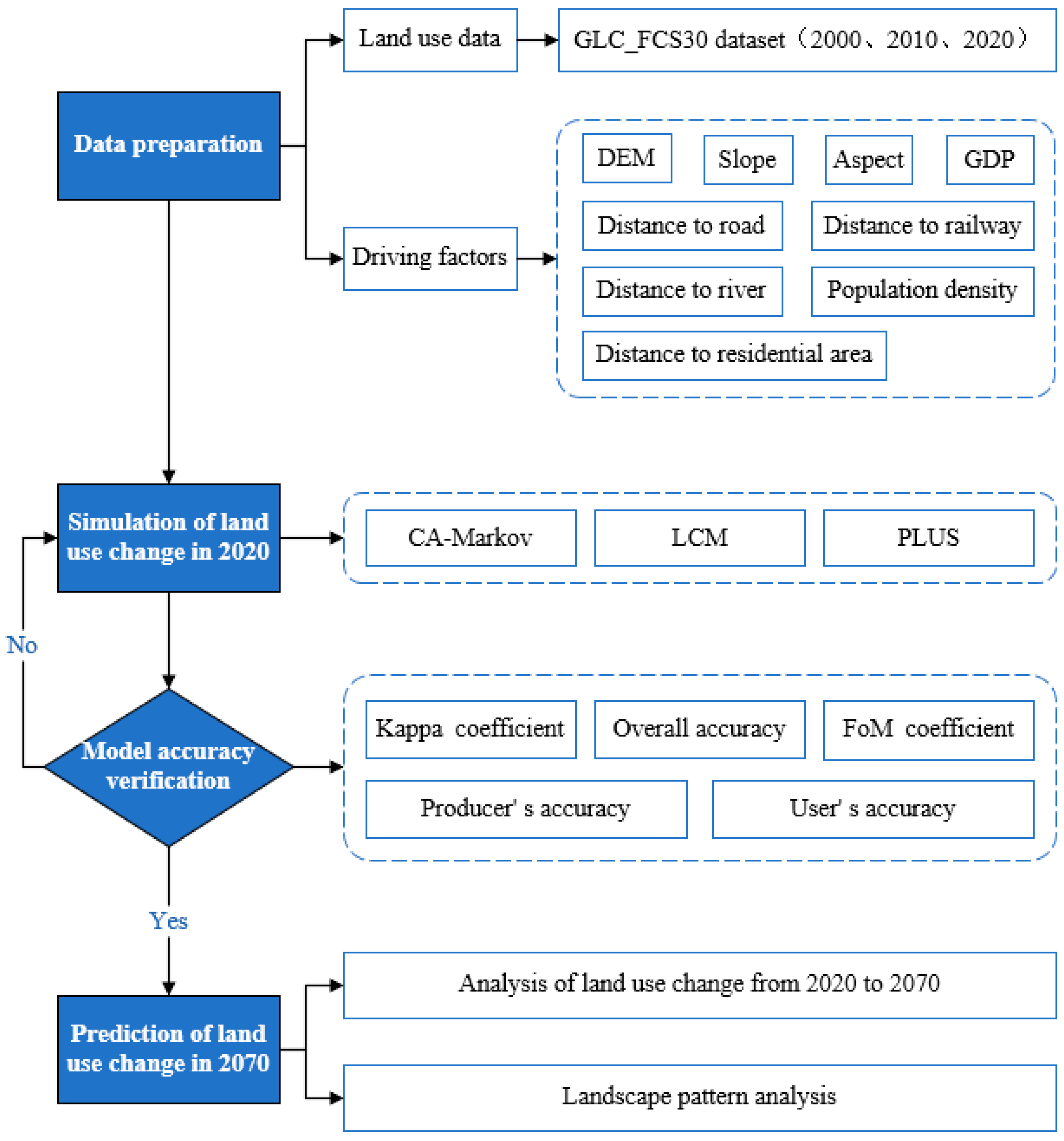
2.2. Technical Route

The technical route of the paper (Figure 2) includes four parts: data preparation, model simulation process, accuracy verification, and future land use prediction.

2.3. Data Source

This paper requires LUCC data and multiple driving factors (Table 1). The LUCC data are the Global Land Cover with Fine Classification System at 30 m (GLC_FCS30) product, with an accuracy of more than 82.5% [27], which can be downloaded from the Chinese Academy of Sciences Data Sharing Service System (https://data.casearth.cn/, accessed on 1 February 2023). The GLC-FCS30 dataset has the advantage of using huge training samples, and this dataset is more advantageous than other land-cover products in terms of spatial detail and land-cover diversity. According to the GLC_FCS30 dataset, the LUCC data area is divided into nine types, namely Cropland (C), forest (F), grassland (GL), shrubland (SL), wetland (WL), water body (WB), impervious surfaces (IS), bare areas (BAs), and permanent ice and snow (PIS). This paper selects nine driving factors (Figure 3) based on reference to the relevant literature and the current situation of this region, namely DEM (km), slope (°), aspect (°), distance to river (Dis1), distance to road (Dis2), distance to railway (Dis3), distance to residential area (Dis4), population density (PD), GDP spatial distribution (GDP). The DEM data is derived from the ASTER GDEM data of the National Aeronautics and Space Administration (NASA), which can be downloaded from the Geospatial Data Cloud (https://www.gscloud.cn/, accessed on 3 February 2023). We can calculate the slope and aspect from the DEM. We can download the water system, data on road and railway, and residential points from the National Catalogue Service for Geographic Information (https://www.webmap.cn/, accessed on 4 February 2023). GDP spatial distribution data (yuan/km2) and population density data (people/km2) were obtained from the Resource and Environment Science and Data Center of the Chinese Academy of Sciences (https://www.resdc.cn/, accessed on 7 February 2023). Before simulating LUCC, we unified the resolution of all raster data to 500 m by resampling, and pre-processed the LUCC data and driving factors with the spatial analysis tools of ArcGIS 10.2 to make the data work properly in the model.

2.4. LULC Simulation Model

2.4.1. CA-Markov Model

The CA-Markov model, which is composed of the cellular automaton (CA) model and the Markov model, can handle spatial information and accurately predict land type transformation [28]. On this basis, this paper introduces the logistic model to calculate the probability of driving factors affecting each land type and the regression relationship between them (Table A1), which is capable of increasing the precision of LUCC simulation [29]. The key steps of the CA-Markov model are: (1) using the Markov model to establish transformation rules and acquire the transfer probability matrix of LUCC, (2) establishing a suitability atlas using logistic regression analysis, and (3) setting the CA filter and cycle number.

2.4.2. Land Change Modeler (LCM)

The LCM is of great value not only for effectively simulating spatial changes in complex systems but also for analyzing the effects of various factors that play a decisive role in land-use changes. The LCM is integrated into the Terr Set software jointly developed by the Clark Laboratory of the United States and the International Conservation Council [30,31]. It is intuitive, easy to use, innovative, and has a wide range of applications for the rapid empirical modeling of LUCC [32]. This paper mainly deals with the components of the LCM, such as the Multi-Layer Perceptron (MLP) neural network, Markov model, and hard prediction model. The main steps of the LCM are (1) analyzing the past LUCC, (2) constructing a potential transformation model using MLP to obtain a potential transfer map, (3) predicting land-use transfer probability using the Markov model, and (4) predicting future LUCC using the hard model.

2.4.3. PLUS Model

The PLUS model is based on raster data and developed by Liang Xun and others at the China University of Geosciences [33]. It is coupled with the land expansion analysis strategy (LEAS) module and the CA model based on the multi-type random patch seeds (CARS) module. It also has unique advantages in simulating the LUCC of patch-level [34]. The steps include: (1) analyzing land expansion and calculating the contribution rate of driving factors to each land type using the LEAS module (Figure A1), (2) calculating land demand using the Markov model, and (3) simulating patch-level LUCC using the CARS module.

2.4.4. Model Validation

This paper uses spatial consistency to compare the differences and consistency of the area and spatial distribution of the simulation results of different models, and the process is mainly realized by the spatial overlay tool of ArcGIS. This paper uses the Kappa coefficient, OA, producer accuracy (PA), and user accuracy (UA) derived from the confusion matrix and introduces the FoM coefficient to check the accuracy. These precision indicators are positively correlated with the precision of the simulation results, and the larger the value of the accuracy indicator, the higher the simulation accuracy. The Kappa coefficient can check the overall consistency between the simulation result and the actual LUCC, and the value is between 0 and 1 [35]. When the Kappa coefficient value is between 0.75 and 1, the consistency between the two results is high, and the simulation accuracy is high [36]. The FoM coefficient can quantitatively test the simulation accuracy at the cell scale, with a value between 0 and 1 [37,38]. The OA measures the validity of the extracted overall data, and its value ranges from 0% to 100% [39]. The result is reliable when the OA value is more excellent than 85%. PA refers to the ratio of correctly classified pixels to the sum of all pixels in the reference verification image, which is used to evaluate whether the study area is accurately classified [40]. UA is the ratio of correctly classified pixels in the classified image to all pixels classified as that class [41]. Both PA and UA range from 0% to 100%.

2.4.5. Landscape Pattern Analysis

Landscape pattern analysis combines different land types in space and expresses their characteristics at the micro-level. Analyzing the landscape pattern can reveal the performance of LUCC at the micro-level and its impact on landscape ecology [42]. The landscape pattern index quantitatively describes the structural composition and spatial relationship of the landscape pattern, which can be divided into three categories: patch metrics, class metrics, and landscape metrics. Because considering that individual patch metrics indexes can only yield landscape information for individual patches, this paper selects landscape pattern indexes at class metrics and landscape metrics. Based on landscape fragmentation, dominance, diversity and uniformity, shape characteristics sprawl, etc., this paper selects the number of patches (NP), patch density (PD), aggregation index (AI), largest patch index (LPI), Shannon’s diversity index (SHDI), Shannon’s evenness index (SHEI), landscape shape index (LSI) and contagion index (CONTAG) [43,44].

3. Results

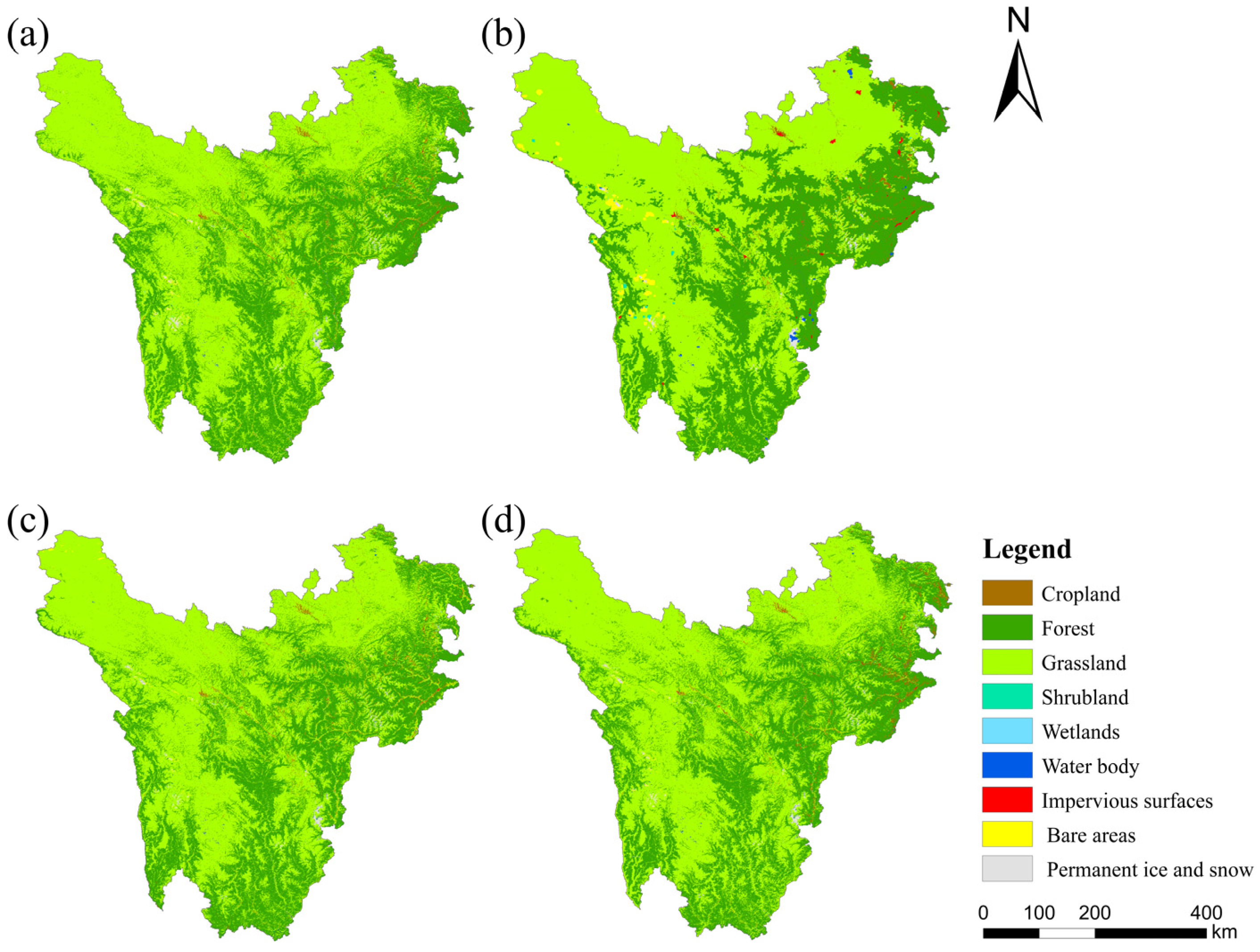
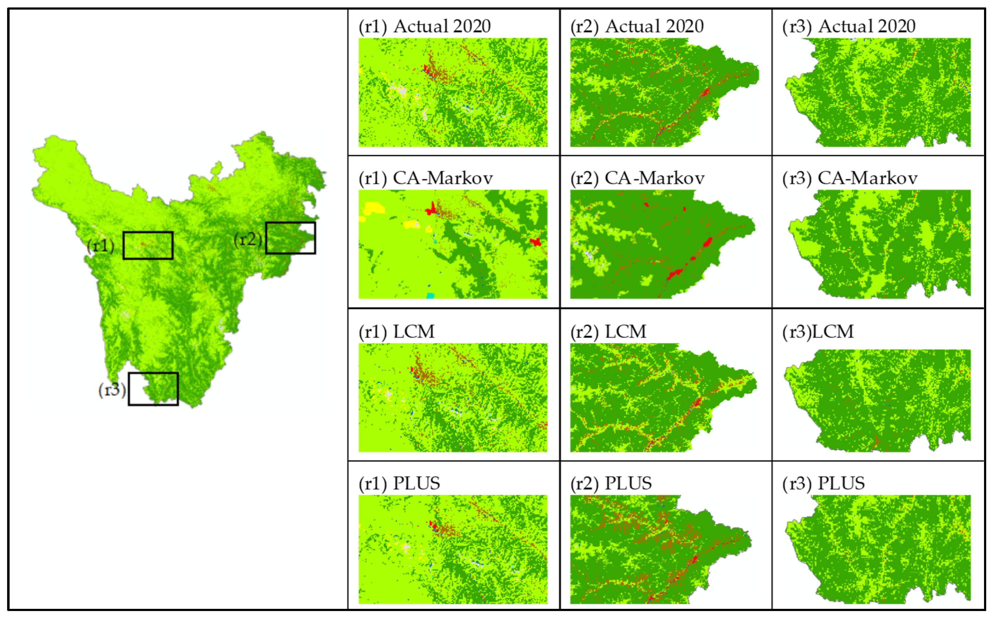
3.1. Comparison of Simulation Results of Different Models

We can compare the simulated LUCC with the actual LUCC area and its proportion in 2020 (Table 2). GL and F are the largest and most widely distributed land types in this region, and the other land types’ areas are much lower than the first two land types (Figure 4). The actual 2020 and simulated LUCC not only show significant similarities in their spatial distribution characteristics, but also in their area ratio. The difference in area ratio between the simulation results and the actual 2020 is less than 2.22% for each land type, and difference area ratios among the three models are all less than 2.70%, showing a good simulation effect.
In order to establish a thorough query of the differences in the spatial distribution of simulated LUCC in detail, we select the northwest, northeast, and south of the Western Sichuan Plateau for local analysis (Figure 5). The simulation result of the CA-Markov model is the most diverse from the real data, and the simulation result of the LCM is closest to the actual 2020.

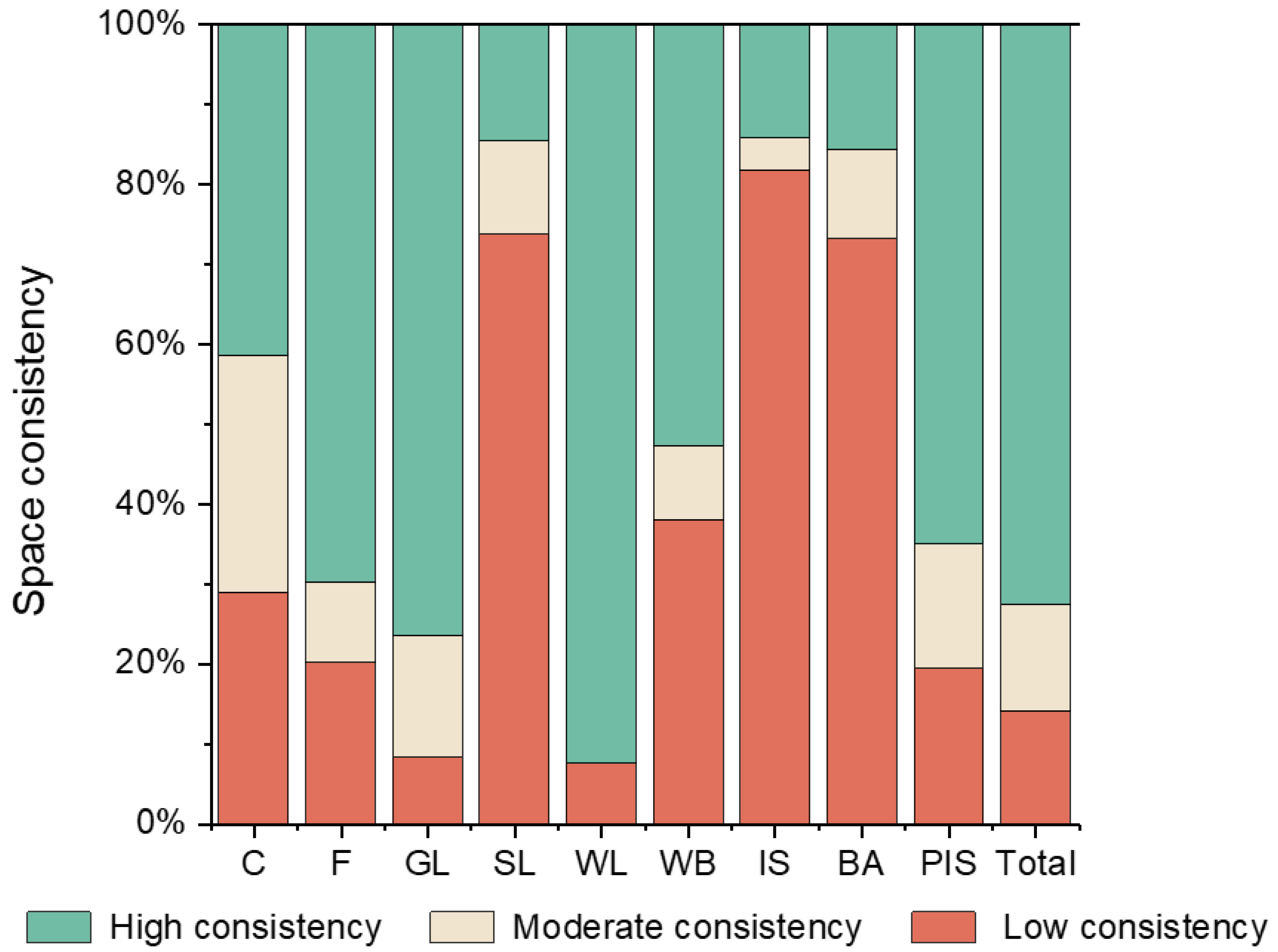
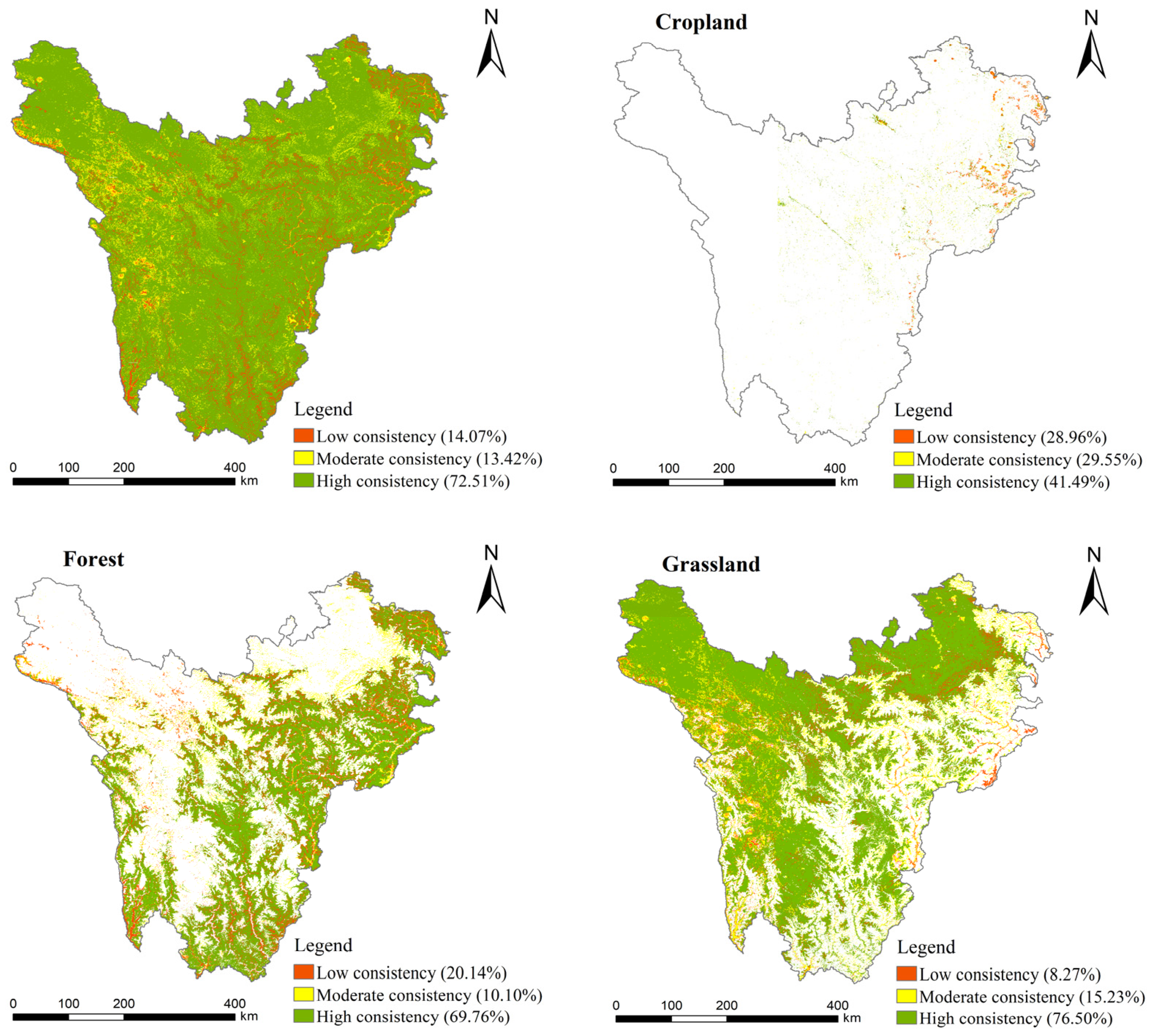
3.2. Comparison of Spatial Consistency of Different Models

The spatial consistency of the simulation results is indicated in red, green, and yellow, respectively (Figure 6 and Figure 7). Green represents the high-consistency region (C1; three models have the same results), yellow represents the medium-consistency region (C2; two models have the same results), red represents the low-consistency region (C3; only one model result is shown), and no data distribution is not shown. The spatial distribution of spatial consistency for the three main land types and the overall LUCC is mainly shown in the paper.
C is primarily distributed in Aba. The C3 area accounts for 28.96% of the total area of C. The area ratios of C2 and C1 are 29.55% and 41.49%, respectively.
F covers a large area and is widely distributed, but it is less distributed in the northwest, north, and west of the study region. The area of C1 accounts for the highest proportion, reaching 69.76%. The proportion of C2 is only 10.10%.
GL is widely distributed in every county. The resolution of the three models for the GL is very high, the C1 area accounts for 76.50%, and the smallest C3 area only accounts for 8.27% of the GL.
The overall spatial consistency of the three models is high. The C3 area accounts for only 14.07%, scattered around the canyons. The area percentage of the C2 is 13.42%. And the area percentage of the C1 is as high as 72.51%, distributed throughout the research region.

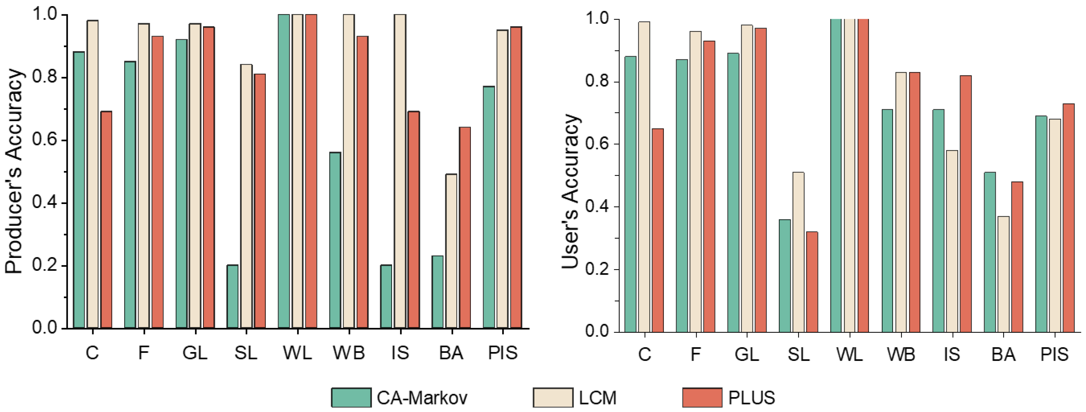
3.3. Accuracy Verification

This paper selects the Kappa coefficient, FoM coefficient, and OA to validate the exactitude of the simulated LUCC (Table 3) and uses UA and PA (Figure A2) for auxiliary discrimination.
The Kappa coefficients of the CA-Markov, LCM, and PLUS model are 0.76, 0.93, and 0.89, respectively. The FoM coefficients are 0.07, 0.21, and 0.15, respectively. The overall accuracies are 0.88, 0.97, and 0.94, respectively. Among the three models, the Kappa coefficient, FoM coefficient, and OA of the LCM model are all the best, indicating that the simulation result of the LCM is closer to the actual situation.

3.4. Predicting Future LUCC

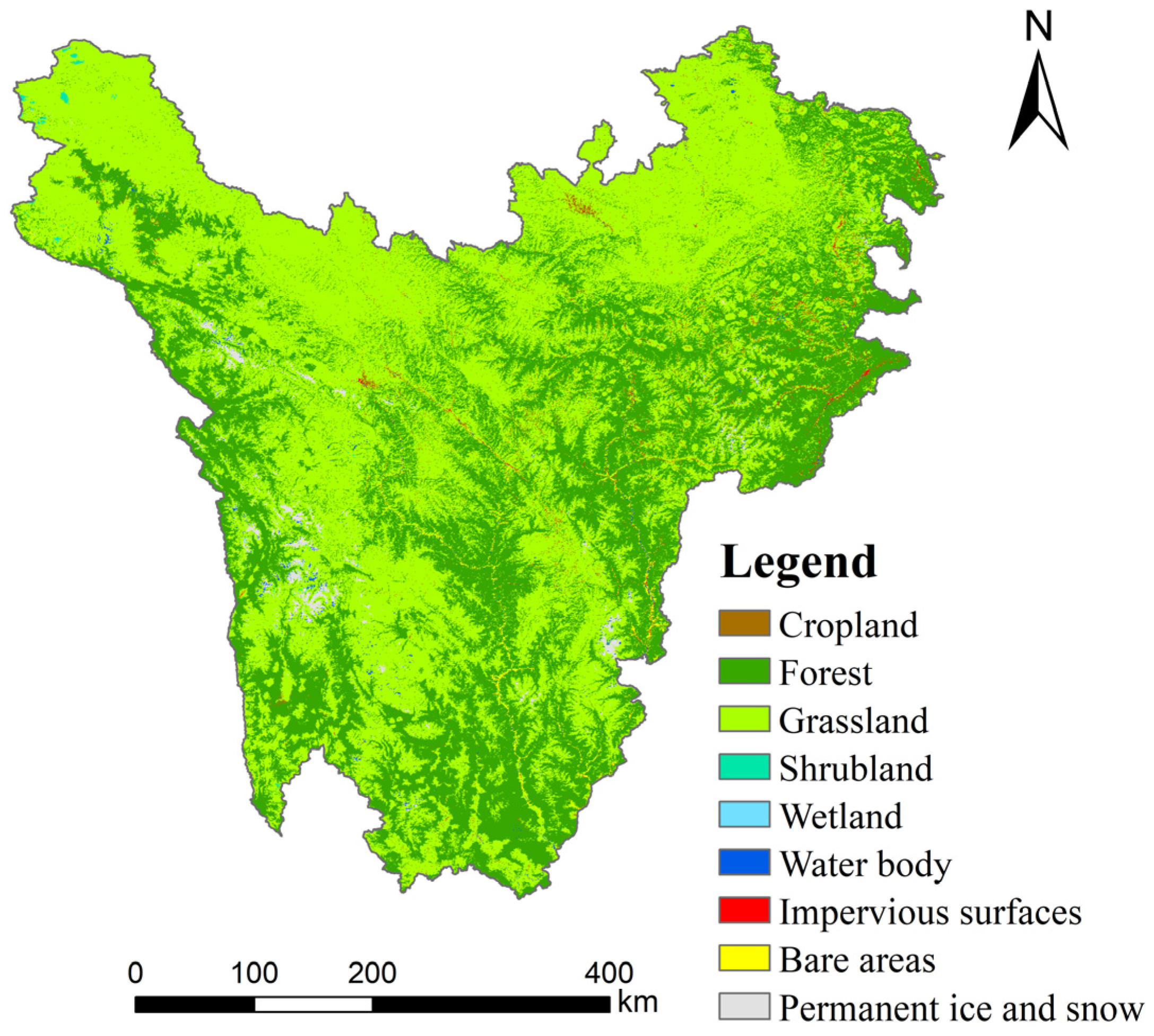
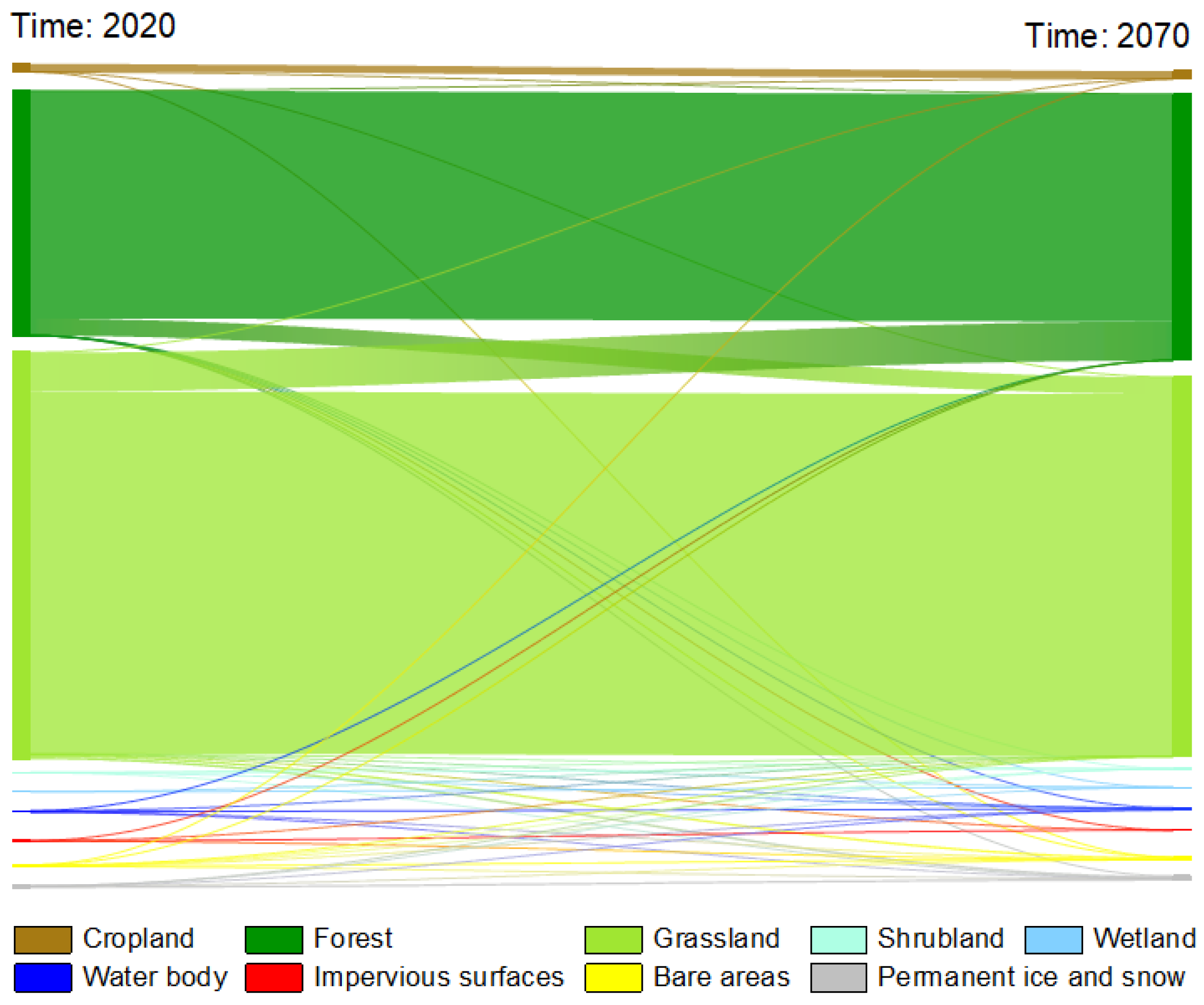
3.4.1. Future LUCC Forecast Analysis

To explore the LUCC of the Western Sichuan Plateau in the future over a long period of time, this paper is based on the merit of the long-term forecast of the Markov model, taking the 2020 LUCC as the initial data, using the LCM to predict the LUCC of 2030, and then iterating for another ten years, and so on, until the 2070 LUCC is simulated.
We can analyze the change in land types through the area and its proportion of the LUCC in 2070 (Table 4, Figure 8) and the sandy map of land-use transfer (Figure 9). Regarding area changes, the area proportion of C changes from 1.19% to 1.29%. F is the second largest land type in the study area, with the area changing from 90,879.52 km2 to 95,648.93 km2. By 2070, GL is still the largest land type, with an area of 143,113.50. The area ratio of SL increases to 0.12%. The area of WL in the region is the smallest, and the area accounts for only 0.01%. The area of the WB has risen 85.29 km2 in 50 years. The area ratioes of IS, BA, and PIS increases by 0.05%, 0.15%, and 0.38%. In terms of the direction of land type transfer, all land types have a tendency to change to different land types.

3.4.2. Analysis of Landscape Pattern Change

Analyzing the landscape indexes at the class metrics (Table 5), it can be seen that, in both 2020 and 2070, the areas of NP and PD of F are the largest. The value of LPI for GL is 52.6044 in 2020 and 49.9947 in 2070. F and GL have the highest AI value of all land types, and WL has the smallest AI value of only 2.9046.
Analysis of the landscape index at the landscape metrics (Table 6) found that the value of NP and PD decreased by 1433 and 0.0059, respectively, the value of AI increased by 0.5929, the value of LSI decreased from 113.6849 in 2020 to 110.7741 in 2070, the value of CONTAG decreased from 68.1057 to 66.5422, and the value of SHDI and SHEI increased by 6.76% and 6.75%, respectively.

4. Discussion

4.1. Model Analysis

In this paper, by simulating the LUCC of the study area in 2020 and comparing its spatial distribution consistency, we found that the overall distribution trend of C is that the further to the northeast of the research region, the lower the consistency. The principal reason for its C3 formation is the difficulty in distinguishing adjacent GL. The F is widely distributed and highly recognizable, with C1 as the main distribution, C2 partly distributed around the highly consistent area, and C3 mainly distributed in the canyon area. The three models have a high recognition of GL, with C1 mainly distributed in areas with gentle topography and C3 distributed primarily in areas bordering F or with obvious topographic relief, such as ravines and mountains. The spatial consistency of the overall landscape is high, and C1 is the largest area in this region. The main reason for the formation of C2 is that the BA and PIS are difficult to distinguish, and the topography of the study is undulating.
Although only a few scholars have explored land use simulation prediction in the western Sichuan plateau, they have achieved credible and reliable results [25,26]. Additionally, a large number of scholars have conducted research and achieved reliable results through the CA-Markov model, PLUS model, and LCM model [45,46,47]. In this study, the Kappa coefficients of the simulation results are all greater than 0.75, and the Kappa coefficient of the LCM even reaches 0.93. The OA of the models are all above 0.85, which shows that the simulation results are highly accurate and effective. The FoM of the LCM is 0.21, which is greater than that of the other two models. Therefore, the LCM has the highest accuracy in this study, and its simulation result is closer to the actual data. Therefore, the accuracy of the result of this paper is also trustworthy compared with these articles.
To date, a large number of scholars have conducted LUCC simulation and prediction studies. The difference between this paper and some studies is that different models are selected to simulate LUCC instead of a single model. The CA-Markov model predicts the land demand of each region through the spatial pattern distribution of the Markov model and calculates the LUCC transfer probability (Table A2) with a relatively simple algorithm. At the same time, logistic regression analysis linearly fits different land types and various driving factors. This creates a suitability atlas through a regression analysis of all factors according to a trend. This method simplifies the analysis process of driving factors in preparing suitability maps. Still, because some land types are relatively scattered in this study, the overall fitting cannot fully show the impact of driving factors on LUCC [29]. Logistic regression also has certain limitations that may lead to errors in the suitability atlas [48], such as the spatial autocorrelation of independent variables, which may be the reason for the low accuracy of the simulation result of the CA-Markov model. In the LCM, before calculating the LUCC transfer probability using the Markov model, the MLP neural network establishes the nonlinear relation between the LUCC and the driving factors through machine learning algorithms to simulate the conversion potential of the LUCC. The MLP neural network has the ability to calibrate, model, and predict the temporal and spatial phenomena of the nonlinear relation between the dependent variable and the independent variable [49,50] and can analyze the position and change trend of the LUCC [51]. The LEAS module of the PLUS model uses the random forest (RF) algorithm to analyze the relation between the expansion results of each category and the driving factors one by one, obtain the conversion rules of each land type, and then obtain the contribution of each factor to the expansion of each category in the period [52]. In the PLUS model, the calculation results of the Markov model show only the land demand of the model. Compared to other algorithms, the RF algorithm is less prone to overfitting problems during the simulation process and has a better prediction ability [53]. The PLUS model and the LCM involve more complex algorithms, and the simulation process is more complicated than that of the CA-Markov model, which may also result in higher accuracy and better simulation results for the two models. Although the simulation results of both the PLUS model and the LCM are good, the lower accuracy of the PLUS model may be because the MLP neural network has a greater advantage in terms of long-term simulation, and the algorithm of the PLUS model has shortcomings compared to the LCM [54]. According to the analysis results in this paper, we summarize the advantages and disadvantages of the three models (Table 7).

4.2. Predicting Future LUCC

In this paper, we used the LCM to predict the LUCC in 2070 in the research area and combined it with landscape pattern analysis. From the perspective of land type transfer in LUCC from 2020 to 2070, there is a trend of shifting to different land types in all regions, and the following land types are more obvious: F is mainly transformed into F and GL, and a tiny part is transferred to IS and BA; GL is mainly converted into C, F, GL, and BA; BA are mainly transformed into GL, BA, and PIS; PIS is mainly transformed into GL, WB, and PIS. In terms of area change, the area of GL decreased, the area of WL remained almost unchanged, and the area of other land types increased. The research area is rich in natural resources, and animal husbandry is relatively developed. Over-harvesting and over-grazing may lead to GL degradation. With the development of society, urbanization is accelerating, and the population is increasing, “human-land conflict” may be one of the reasons for the decrease in GL area. In recent years, the Forestry Bureau in the Western Sichuan Plateau has actively carried out ecological restoration and strengthened the protection of forest resources. This measure is also likely to lead to a reduction in grassland area and increase in forest area. Although long-term ecological protection measures are needed to restore forest resources, it can be seen from Figure 9 that GL will be transformed into F from 2020 to 2070, which proves that these protection measures are effective.
According to the landscape index analysis of the class metrics, the changes in the PD and NP of each land type were similar from 2020 to 2070, with F and GL decreasing, WL remaining unchanged, and other land types increasing. The meaning of AI is similar to that of NP and PD, and both can indicate the degree of fragmentation and dispersion of the landscape. According to the changes in the major categories of AI from 2020 to 2070, the fragmentation of land types other than C, WL, and IS is weakening, and the spatial distribution is also becoming more concentrated. LPI can describe the dominance of land types. In 2020 and 2070, F and GL will occupy a dominant position in the entire landscape. The LPI of SL, WB, BA, and PIS cover is increasing, indicating that the dominance of these land types is increasing. Analyzing the landscape indexes at the landscape metrics, it can be seen that the NP and PD of the landscape are decreasing while the AI is increasing, indicating that the degree of fragmentation of the overall landscape is decreasing and the degree of aggregation is increasing. The reduction in LSI indicates that the complexity of the landscape is decreasing. The reduction in CONTAG indicates that the degree of land scape extension has decreased. The increase in SHDI and SHEI shows that the various landscape types in this region are developing in an orderly and reasonable manner, the diversity and uniformity have been improved, and the richness has been improved.

4.3. Disadvantages and Limitations

When analyzing the impact of driving factors on LUCC, this paper only consideres some natural factors and socioeconomic factors, and does not think about the impact of climate data, such as temperature, as well as the constraints on LUCC, such as policy formulation and protected areas. This paper explores the development trend of LUCC in the western Sichuan Plateau from 2020 to 2070 based on a natural development scenario without policy constraints. In subsequent studies, it is more practical to explore the spatial distribution pattern of LUCC under different scenarios by setting different simulation scenarios.
At present, most LUCC simulation studies use a single land use simulation model. However, dissimilar models have various algorithms, different benefits and different shortcomings, and different results can be obtained [55]. Therefore, using multiple different LUCC simulation models in the same region is beneficial to regional LUCC simulation research and is more conducive to the selection of a model that is suitable for this region. Although this paper selects three different models for simulation and prediction, it is not enough for multi-model comparison and analysis, and more models need to be considered for comparison in future research. Although the simulation results in this paper can meet the basic demands, there is still a certain gap with reality. In future research, some parameters can be added to the model, or multiple land use models can be coupled to combine different advantages to improve the simulation accuracy [56].

5. Conclusions

We used the CA-Markov model, LCM, and PLUS model to simulate the land use status of the western Sichuan plateau in 2020, compare their results with the actual situation, and verify the accuracy. The LCM with the highest accuracy in the simulation result was selected to explore the development trend of LUCC structure in the future to supply theoretical support for the optimal management of land, social economy, and ecological protection of the Western Sichuan Plateau. The major conclusions of this article include three points:
(1) The simulation results of the three models have high similarity in spatial distribution, with a Kappa coefficient of 0.89, FoM coefficient of 0.15, and OA of 0.94 for the LCM, and the simulation accuracy is higher than that of the PLUS model and CA-Markov model. However, for different land types, the PA and UA of the three models have significant variability.
(2) Using the LCM to simulate the change in LUCC and landscape pattern from 2020 to 2070 showed that, except for GL and WL, the area of other land types is increasing, and the area of GL is reduced by 6699.25 km2, but is still the largest. The proportion of WL remained unchanged, and the area decreased by only 0.39 km2. In terms of land transfer, there is a tendency to shift to different land types in different regions. Except for C, WL, and BA, the fragmentation of other land types is decreasing. F and GL are becoming less dominant but still dominate the landscape. The degree of aggregation of the overall landscape increased, the degree of complexity decreased, and the diversity, uniformity, and richness of each landscape type increased, showing an orderly and reasonable development.
(3) We can assess the future evolution of land through the predicted LUCC in 2070, which can provide decision-making advice regarding land use for the government. With the over-exploitation and utilization of natural resources, problems such as GL degradation and weakening of the ecological automatic adjustment function may arise. Various ecological protection and restoration measures have been implemented on the Western Sichuan Plateau. We should strictly observe the policies of ecological protection areas and basic protection farmland when planning land in the future, and protect ecological resources such as forest, grassland and cropland. We also need to consider high-quality developments that combine economic benefits and ecological security.

Author Contributions

Conceptualization, J.X. and K.H.; methodology, X.Y. and J.X.; formal analysis, X.Y.; investigation, Y.L. (Yuanyuan Li), Y.L. (Yang Lin) and G.Q.; resources, J.X.; writing—original draft preparation, X.Y.; writing—review and editing, J.X., K.H., T.L. and P.R.; project administration, X.Y. and J.X.; funding acquisition, J.X. and P.R. All authors have read and agreed to the published version of the manuscript.

Funding

This research is supported by the Sichuan Science and Technology Program (2023NSFSC1979, 2023NSFSC0191), and the National Natural Science Foundation of China (41801185).

Data Availability Statement

All data can be accessed through the provided website.

Acknowledgments

We would like to thank to the editors and reviewers, who have put great effort into their comments on this manuscript.

Conflicts of Interest

The authors declare no conflict of interest.

Appendix A

Table A1. Results of logistic regression analysis of land use drivers.
IFIndexFGLSLWLWBISBAPIS
DEMβ--0.00037 ---0.00016 −0.00023
exp(β)--1.00037 ---1.00016 0.99977
Slopeβ0.01703 −0.01698 -0.04955 --0.00681 0.01875
exp(β)1.01718 0.98316 -1.05080 --1.00683 1.01893
Aspectβ--−0.00171 -----
exp(β)--0.99829 -----
Dis1β−0.00002 0.00001 0.00025 0.00032 −0.00032 −0.00291 0.00028 0.00060
exp(β)0.99998 1.00001 1.00025 1.00032 0.99968 0.99709 1.00028 1.00060
Dis2β−0.00005 0.00005 -0.00006 −0.00003 −0.00082 -0.00003
exp(β)0.99995 1.00005 -1.00006 0.99998 0.99919 -1.00003
Dis3β0.00000 0.00000 0.00000 −0.00001 0.00000 −0.00001 0.00001 0.00000
exp(β)1.00000 1.00000 1.00000 0.99999 1.00000 1.00000 1.00001 1.00000
Dis4β−0.00006 0.00006 0.00005 -0.00006 −0.00040 0.00015 0.00019
exp(β)0.99994 1.00006 1.00005 -1.00006 0.99960 1.00015 1.00019
PDβ0.03696 −0.05085 -0.07230 0.04630 -0.02854 0.07462
exp(β)1.03765 0.95042 -1.07498 1.04739 -1.02895 1.07748
GDPβ−0.00003 0.00003 --0.00002 -−0.00020 −0.00013
exp(β)0.99997 1.00003 --1.00002 -0.99980 0.99987
Constantβ0.55677 −0.51204 −2.62761 −1.49221 −0.51878 5.96395 −5.06016 −4.48808
exp(β)1.74502 0.59927 0.07225 0.22488 0.59525 389.14307 0.00635 0.01124
Dis1: distance to river; Dis2: distance to road; Dis3: distance to railway; Dis4: distance to residential area; PD: population density; GDP: GDP spatial distribution. IF: impact factor. “-”: no participating in the construction of the equation. Full names of abbreviations are listed in Table 2 and Table A1.
Figure A1. The contribution rate of influence factors to each land type. (ai): C, F, GL, SL, WL, WB, IS, BA, PIS. Full names of abbreviations are listed in Table 2 and Table A1.
Remotesensing 15 03629 g0a1
Table A2. The LUCC transition probability matrix from 2010 to 2020 based on the Markov model.
CFGLSLWLWBISBAPIS
C0.98750.00300.0056000.00040.00340.00010
F0.00010.98570.0139000.00010.00010.00010
GL0.00020.00900.98930.000100.00010.00020.00100.0001
SL00.16670.12420.68630000.00650.0163
WL000010000
WB000001000
IS000000100
BA00.00380.25600.015500.034500.66250.0276
PIS00.00140.04160.000700.006800.02280.9267
Full names of abbreviations are listed in Table 2.
Figure A2. PA (left) and UA (right) for different classes in different models in 2020. Full names of abbreviations are listed in Table 2.
Remotesensing 15 03629 g0a2

References

  1. Steffen, W.; Sanderson, A.; Tyson, P.; Jäger, J.; Matson, P.; Moore, B.; Oldfield, F.; Richardson, K.; Schellnhuber, H.J.; Turner, B.L.; et al. Global Change and the Earth System: A Planet Under Pressure; Springer: Berlin/Heidelberg, Germany, 2005. [Google Scholar]
  2. Zhang, H.; Zhang, B. A review of international land use/cover change modeling studies. J. Nat. Resour. 2005, 20, 422–431. [Google Scholar]
  3. Dai, E.; Ma, L. A Review of Land Change Modeling Methods. Prog. Geogr. 2018, 37, 152–162. [Google Scholar] [CrossRef] [Green Version]
  4. Veldkamp, A.; Lambinb, E.F. Predicting land-use change. Agric. Ecosyst. Environ. 2001, 85, 1–6. [Google Scholar] [CrossRef]
  5. Jiao, M.; Hu, M.; Xia, B. Spatiotemporal dynamic simulation of land-use and landscape-pattern in the Pearl River Delta, China. Sustain. Cities Soc. 2019, 49, 101581. [Google Scholar] [CrossRef]
  6. López, E.; Bocco, G.; Mendoza, M.; Duhau, E. Predicting land-cover and land-use change in the urban fringe: A case in Morelia city, Mexico. Landsc. Urban Plan. 2001, 55, 271–285. [Google Scholar] [CrossRef]
  7. Geng, B.; Zheng, X.; Fu, M. Scenario analysis of sustainable intensive land use based on SD model. Sustain. Cities Soc. 2017, 29, 193–202. [Google Scholar] [CrossRef]
  8. Liu, X.; Ou, J.; Li, X.; Ai, B. Combining system dynamics and hybrid particle swarm optimization for land use allocation. Ecol. Model. 2013, 257, 11–24. [Google Scholar] [CrossRef]
  9. Baker, W.L. A review of models of landscape change. Landsc. Ecol. 1989, 2, 111–133. [Google Scholar] [CrossRef]
  10. Yu, D.; Procopio, N.A.; Fang, C. Simulating the Changes of Invasive Phragmites australis in a Pristine Wetland Complex with a Grey System Coupled System Dynamic Model: A Remote Sensing Practice. Remote Sens. 2022, 14, 3886. [Google Scholar] [CrossRef]
  11. Huang, Z.; Li, X.; Du, H.; Mao, F.; Han, N.; Fan, W.; Xu, Y.; Luo, X. Simulating Future LUCC by Coupling Climate Change and Human Effects Based on Multi-Phase Remote Sensing Data. Remote Sens. 2022, 14, 1698. [Google Scholar] [CrossRef]
  12. Gomes, E.; Inácio, M.; Bogdzevič, K.; Kalinauskas, M.; Karnauskaitė, D.; Pereira, P. Future land-use changes and its impacts on terrestrial ecosystem services: A review. Sci. Total Environ. 2021, 781, 146716. [Google Scholar] [CrossRef]
  13. Verburg, P.H.; Soepboer, W.; Veldkamp, A.; Limpiada, R.; Espaldon, V.; Mastura, S.S.A. Modeling the spatial dynamics of regional land use: The CLUE-S model. Environ. Manag. 2002, 30, 391–405. [Google Scholar] [CrossRef]
  14. Hao, L.; He, S.; Zhou, J.; Zhao, Q.; Lu, X. Prediction of the landscape pattern of the Yancheng Coastal Wetland, China, based on XGBoost and the MCE-CA-Markov model. Ecol. Indic. 2022, 145, 109735. [Google Scholar] [CrossRef]
  15. Wei, Q.; Abudureheman, M.; Halike, A.; Yao, K.; Yao, L.; Tang, H.; Tuheti, B. Temporal and spatial variation analysis of habitat quality on the PLUS-InVEST model for Ebinur Lake Basin, China. Ecol. Indic. 2022, 145, 109632. [Google Scholar] [CrossRef]
  16. Wang, Z.; Song, W.; Yin, L. Responses in ecosystem services to projected land cover changes on the Tibetan Plateau. Ecol. Indic. 2022, 142, 109228. [Google Scholar] [CrossRef]
  17. Liu, D.; Zhenga, X.; Wang, H. Land-use Simulation and Decision-Support system (LandSDS)_ Seamlessly integrating system dynamics, agent-based model, and cellular automata. Ecol. Model. 2020, 417, 108924. [Google Scholar] [CrossRef]
  18. Bao, S.; Yang, F. Spatio-Temporal Dynamic of the Land Use/Cover Change and Scenario Simulation in the Southeast Coastal Shelterbelt System Construction Project Region of China. Sustainability 2022, 14, 8952. [Google Scholar] [CrossRef]
  19. Zhang, P.; Liu, L.; Yang, L.; Zhao, J.; Li, Y.; Qi, Y.; Ma, X.; Cao, L. Exploring the response of ecosystem service value to land use changes under multiple scenarios coupling a mixed-cell cellular automata model and system dynamics model in Xi’an, China. Ecol. Indic. 2023, 147, 110009. [Google Scholar] [CrossRef]
  20. Chen, Z.; Huang, M.; Zhu, D.; Altan, O. Integrating Remote Sensing and a Markov-FLUS Model to Simulate Future Land Use Changes in Hokkaido, Japan. Remote Sens. 2021, 13, 2621. [Google Scholar] [CrossRef]
  21. Fu, F.; Deng, S.; Wu, D.; Liu, W.; Bai, Z. Research on the spatiotemporal evolution of land use landscape pattern in a county area based on CA-Markov model. Sustain. Cities Soc. 2022, 80, 103760. [Google Scholar] [CrossRef]
  22. Motlagh, S.K.; Sadoddin, A.; Haghnegahdar, A.; Razavi, S.; Salmanmahiny, A.; Ghorbani, K. Analysis and prediction of land cover changes using the land change modeler (LCM) in a semiarid river basin, Iran. Land Degrad. Dev. 2021, 32, 3092–3105. [Google Scholar] [CrossRef]
  23. Gao, L.; Tao, F.; Liu, R.; Wang, Z.; Leng, H.; Zhou, T. Multi-scenario simulation and ecological risk analysis of land use based on the PLUS model: A case study of Nanjing. Sustain. Cities Soc. 2022, 85, 104055. [Google Scholar] [CrossRef]
  24. Wei, J.; Hu, A.; Gan, X.; Zhao, X.; Huang, Y. Spatial and Temporal Characteristics of Ecosystem Service Trade-Off and Synergy Relationships in the Western Sichuan Plateau, China. Forests 2022, 13, 1845. [Google Scholar] [CrossRef]
  25. Li, W.; Xiang, M.; Duan, L.; Liu, Y.; Yang, X.; Mei, H.; Wei, Y.; Zhang, J.; Deng, L. Simulation of land utilization change and ecosystem service value evolution in Tibetan area of Sichuan Province. Alex. Eng. J. 2023, 70, 13–23. [Google Scholar] [CrossRef]
  26. Xiang, M.; Yang, J.; Li, W.; Song, Y.; Wang, C.; Liu, Y.; Liu, M.; Tan, Y. Spatiotemporal Evolution and Simulation Prediction of Ecosystem Service Function in the Western Sichuan Plateau Based on Land Use Changes. Front. Environ. Sci. 2022, 10, 391. [Google Scholar] [CrossRef]
  27. Zhang, X.; Liu, L.; Chen, X.; Gao, Y.; Xie, S.; Mi, J. GLC_FCS30: Global land-cover product with fine classification system at 30 m using time-series Landsat imagery. Earth Syst. Sci. Data 2021, 13, 2753–2776. [Google Scholar] [CrossRef]
  28. Ou, D.; Zhang, Q.; Tang, H.; Qin, J.; Yu, D.; Deng, O.; Gao, X.; Liu, T. Ecological spatial intensive use optimization modeling with framework of cellular automata for coordinating ecological protection and economic development. Sci. Total Environ. 2023, 857, 159319. [Google Scholar] [CrossRef]
  29. Guan, D.; Zhao, Z.; Tan, J. Dynamic simulation of land use change based on logistic-CA-Markov and WLC-CA-Markov models. Environ. Sci. Pollut. Res. 2019, 26, 20669–20688. [Google Scholar] [CrossRef]
  30. Eastman, J.R.; Toledano, J. A short presentation of the Land Change Modeler (LCM). In Geomatic Approaches for Modeling Land Change Scenarios; Springer: Berlin/Heidelberg, Germany, 2018; pp. 499–505. [Google Scholar] [CrossRef]
  31. Mas, J.-F.; Kolb, M.; Paegelow, M.; Olmedo, M.T.C.; Houet, T. Modelling Land use/cover changes: A comparison of conceptual approaches and softwares. Environ. Model. Softw. 2014, 51, 94–111. [Google Scholar] [CrossRef] [Green Version]
  32. Ansari, A.; Golabi, M.H. Prediction of spatial land use changes based on LCM in a GIS environment for Desert Wetlands—A case study: Meighan Wetland, Iran. Int. Soil Water Conserv. Res. 2019, 7, 64–70. [Google Scholar] [CrossRef]
  33. Liang, X.; Guan, Q.; Clarke, K.C.; Liu, S.; Wang, B.; Yao, Y. Understanding the drivers of sustainable land expansion using a patch-generating land use simulation (PLUS) model: A case study in Wuhan, China. Comput. Environ. Urban Syst. 2021, 85, 101569. [Google Scholar] [CrossRef]
  34. Deng, Z.; Quan, B. Intensity Characteristics and Multi-Scenario Projection of Land Use and Land Cover Change in Hengyang, China. Int. J. Environ. Res. Public Health 2022, 19, 8491. [Google Scholar] [CrossRef] [PubMed]
  35. Cohen, J. A coefficient of agreement for nominal scales. Educ. Psychol. Meas. 1960, 20, 37–46. [Google Scholar] [CrossRef]
  36. Jafari, R.; Abedi, M. Remote sensing-based biological and nonbiological indices for evaluating desertification in Iran: Image versus field indices. Land Degrad. Dev. 2021, 32, 2805–2822. [Google Scholar] [CrossRef]
  37. Pontius, R.G., Jr.; Boersma, W.; Castella, J.-C.; Clarke, K.; de Nijs, T.; Dietzel, C.; Duan, Z.; Fotsing, E.; Goldstein, N.; Kok, K.; et al. Comparing the input, output, and validation maps for several models of land chang. Ann. Reg. Sci. 2008, 42, 11–37. [Google Scholar] [CrossRef] [Green Version]
  38. Qian, Y.; Xing, W.; Guan, X.; Yang, T.; Wu, H. Coupling cellular automata with area partitioning and spatiotemporal convolution for dynamic land use change simulation. Sci. Total Environ. 2020, 722, 137738. [Google Scholar] [CrossRef]
  39. Marzialetti, F.; Gamba, P.; Sorriso, A.; Carranza, M.L. Monitoring Urban Expansion by Coupling Multi-Temporal Active Remote Sensing and Landscape Analysis: Changes in the Metropolitan Area of Cordoba (Argentina) from 2010 to 2021. Remote Sens. 2023, 15, 336. [Google Scholar] [CrossRef]
  40. Sun, L.; Schulz, K. The Improvement of Land Cover Classification by Thermal Remote Sensing. Remote Sens. 2015, 7, 8368–8390. [Google Scholar] [CrossRef] [Green Version]
  41. Senf, C.; Leitão, P.J.; Pflugmacher, D.; Linden, S.V.D.; Hostert, P. Mapping land cover in complex Mediterranean landscapes using Landsat: Improved classification accuracies from integrating multi-seasonal and synthetic imagery. Remote Sens. Environ. 2015, 156, 527–536. [Google Scholar] [CrossRef]
  42. Griffith, J.A. The role of landscape pattern analysis in understanding concepts of land cover change. J. Geogr. Sci. 2004, 14, 3–17. [Google Scholar] [CrossRef]
  43. Rutledge, D. Landscape Indices as Measures of the Effects of Fragmentation: Can Pattern Reflect Process? DOC Science Internal Series; Department of Conservation: Wellington, New Zealand, 2003.
  44. Haines-Young, R.; Chopping, M. Quantifying landscape structure: A review of landscape indices and their application to forested landscapes. Prog. Phys. Geogr. Earth Environ. 1996, 20, 418–445. [Google Scholar] [CrossRef]
  45. Mansour, S.; Al-Belushi, M.; Al-Awadhi, T. Monitoring land use and land cover changes in the mountainous cities of Oman using GIS and CA-Markov modelling techniques. Land Use Policy 2020, 91, 104414. [Google Scholar] [CrossRef]
  46. Wang, Q.; Wang, H. An integrated approach of logistic-MCE-CA-Markov to predict the land use structure and their micro-spatial characteristics analysis in Wuhan metropolitan area, Central China. Environ. Sci. Pollut. Res. 2022, 29, 30030–30053. [Google Scholar] [CrossRef] [PubMed]
  47. Sahle, M.; Saito, O.; Fürst, C.; Demissew, S.; Yeshitela, K. Future land use management effects on ecosystem services under different scenarios in the Wabe River catchment of Gurage Mountain chain landscape, Ethiopia. Sustain. Sci. 2018, 14, 175–190. [Google Scholar] [CrossRef]
  48. Arsanjani, J.J.; Helbich, M.; Kainz, W.; Boloorani, A.D. Integration of logistic regression, Markov chain and cellular automata models to simulate urban expansion. Int. J. Appl. Earth Obs. Geoinf. 2013, 21, 265–275. [Google Scholar] [CrossRef]
  49. Gaur, S.; Mittal, A.; Bandyopadhyay, A.; Holman, I.; Singh, R. Spatio-temporal analysis of land use and land cover change: A systematic model inter-comparison driven by integrated modelling techniques. Int. J. Remote Sens. 2010, 41, 9229–9255. [Google Scholar] [CrossRef]
  50. Shahi, E.; Karimi, S.; Jafari, H.R. Monitoring and modeling land use/cover changes in Arasbaran protected Area using and integrated Markov chain and artificial neural network. Model. Earth Syst. Environ. 2020, 6, 1901–1911. [Google Scholar] [CrossRef]
  51. Alqadhi, S.; Mallick, J.; Balha, A.; Bindajam, A.; Singh, C.K.; Hoa, P.V. Spatial and decadal prediction of land use/land cover using multi-layer perceptron-neural network (MLP-NN) algorithm for a semi-arid region of Asir, Saudi Arabia. Earth Sci. Inform. 2021, 14, 1547–1562. [Google Scholar] [CrossRef]
  52. Ma, G.; Li, Q.; Zhang, J.; Zhang, L.; Cheng, H.; Ju, Z.; Sun, G. Simulation and Analysis of Land-Use Change Based on the PLUS Model in the Fuxian Lake Basin (Yunnan–Guizhou Plateau, China). Land 2022, 12, 120. [Google Scholar] [CrossRef]
  53. Lin, Z.; Peng, S. Comparison of multimodel simulations of land use and land cover change considering integrated constraints—A case study of the Fuxian Lake basin. Ecol. Indic. 2022, 142, 109254. [Google Scholar] [CrossRef]
  54. Xu, L.; Liu, X.; De, T.; Liu, Z.; Yin, L.; Zheng, W. Forecasting Urban Land Use Change Based on Cellular Automata and the PLUS Model. Land 2022, 11, 652. [Google Scholar] [CrossRef]
  55. Luo, G.; Yin, C.; Chen, X.; Xu, W.; Lu, L. Combining system dynamic model and CLUE-S model to improve land use scenario analyses at regional scale: A case study of Sangong watershed in Xinjiang, China. Ecol. Complex. 2010, 7, 198–207. [Google Scholar] [CrossRef]
  56. Zhao, X.; Wang, P.; Gao, S.; Yasir, M.; Islam, Q.U. Combining LSTM and PLUS Models to Predict Future Urban Land Use and Land Cover Change: A Case in Dongying City, China. Remote Sens. 2023, 15, 2370. [Google Scholar] [CrossRef]
Figure 1. Geographical location of the study area. Map of China and Tibetan Plateau from the Resource and Environment Science and Data Center of the Chinese Academy of Sciences.
Remotesensing 15 03629 g001
Figure 2. Technical route.
Remotesensing 15 03629 g002
Figure 3. Driving factors of LUCC.
Remotesensing 15 03629 g003
Figure 4. (a) LUCC in actual 2020, (b) LUCC simulated by CA-Markov model, (c) LUCC simulated by LCM, (d) LUCC simulated by PLUS model.
Remotesensing 15 03629 g004
Figure 5. The simulated LUCC in four sub-regions in the study area are compared using the CA-Markov model, LCM, and PLUS model. The explanation for colored areas in the figure is listed in Figure 4.
Remotesensing 15 03629 g005
Figure 6. Percentage of the spatial consistency area of each land type. Full names of abbreviations are listed in Table 2.
Remotesensing 15 03629 g006
Figure 7. Comparison of spatial consistency between the overall and selected C, F and GL.
Remotesensing 15 03629 g007
Figure 8. LUCC forecast map in 2070.
Remotesensing 15 03629 g008
Figure 9. Sandy map of land use transfer in the Western Sichuan Plateau from 2020 to 2070.
Remotesensing 15 03629 g009
Table 1. Details of LUCC, driving factors’ data.
Data TypeData NameData SourceResolution
Natural factorsthe LUCC dataGLC_FCS30 dataset30 m
DEMthe Geospatial Data Cloud30 m
SlopeCalculated from DEM30 m
Aspect
RiverThe National Catalogue Service
For Geographic Information
-
Socioeconomic factorsRailwayThe National Catalogue Service
For Geographic Information
-
Road
Residential points-
Population densityThe Resource and Environment Science and Data Center of the Chinese Academy of Sciences1000 m
GDP spatial distribution1000 m
Table 2. The area and proportion of each land type in actual 2020 and different models.
Land-Use TypeArea/
Proportion
Actual 2020CA-MarkovLCMPLUS
CArea/km22933.45 2784.23 2948.77 3142.64
Proportion/%1.19%1.13%1.20%1.28%
FArea/km290,879.52 94,450.67 90,004.03 90,001.01
Proportion/%36.94%38.39%36.59%36.58%
GLArea/km2149,812.75 144,596.69 151,249.36 150,985.72
Proportion/%60.90%58.78%61.48%61.37%
SLArea/km2108.99 247.85 64.55 61.11
Proportion/%0.04%0.10%0.03%0.02%
WLArea/km227.63 27.36 25.81 25.81
Proportion/%0.01%0.01%0.01%0.01%
WBArea/km2544.97 707.79 494.80 484.00
Proportion/%0.22%0.29%0.20%0.20%
ISArea/km298.32 457.94 62.65 103.71
Proportion/%0.04%0.19%0.03%0.04%
BAArea/km2743.59 1997.69 520.65 506.41
Proportion/%0.30%0.81%0.21%0.21%
PISArea/km2863.50 742.50 642.11 702.31
Proportion/%0.35%0.30%0.26%0.29%
Total Area/km2246,012.72 246,012.72 246,012.72 246,012.72
C: cropland; F: forest; GL: grassland; SL: shrubland; WL: wetland; WB: water body; IS: impervious surfaces; BA: bare areas; PIS: permanent ice and snow.
Table 3. Accuracy comparison of different models of LUCC in 2020.
CA-MarkovLCMPLUS
Kappa0.760.930.89
OA0.880.970.94
FoM0.070.210.15
Table 4. The area and proportion of land types in LUCC in 2020 and 2070.
LUCC TypeArea/
Proportion
Actual 2020Simulation 2070
CArea/km22933.45 3070.63
Proportion/%1.19%1.29%
FArea/km290,879.52 95,648.93
Proportion/%36.94%38.88%
GLArea/km2149,812.75 143,113.50
Proportion/%60.90%58.17%
SLArea/km2108.99 306.59
Proportion/%0.04%0.12%
WLArea/km227.63 27.24
Proportion/%0.01%0.01%
WBArea/km2544.97 630.26
Proportion/%0.22%0.26%
ISArea/km298.32 222.04
Proportion/%0.04%0.09%
BAArea/km2743.59 1102.98
Proportion/%0.30%0.45%
PISArea/km2863.50 1790.55
Proportion/%0.35%0.73%
Total Area/km2246,012.72 246,012.72
Full names of abbreviations are listed in Table 2.
Table 5. Landscape index calculated at class metrics.
Landscape
Index
YearCFGLSLWLWBISBAPIS
NP (n)2020828214,518945045511917452781656838
2070873213,5806995551119225532819581440
PD (n/100 ha)20200.0337 0.0590 0.0384 0.0018 0.0005 0.0071 0.0011 0.0067 0.0034
20700.03550.05520.02840.00220.00050.00920.00150.00800.0059
LPI (%) 20200.0199 24.7708 52.6044 0.0006 0.0004 0.0023 0.0026 0.0108 0.0485
20700.019923.405949.99470.01450.00040.00600.00260.02040.0841
AI (%)202015.8997 73.2543 82.4134 5.4860 2.9046 12.1744 15.0485 22.4496 47.5178
207015.887076.033682.463640.33642.904617.108415.048525.981453.1743
Full names of abbreviations are listed in Table 2. n: number of patches.
Table 6. Landscape index calculated at landscape metrics.
TimeNP (n)PD (n/100 ha)LSICONTAG (%)SHDI SHEIAI (%)
202037,3410.1518113.684968.10570.79740.362977.4706
207035,9080.1459110.774166.54220.85130.387478.0635
n: number of patches.
Table 7. Summary of the advantages and disadvantages of the three models from this research.
CA-MarkovLCMPLUS
AdvantagesSimple algorithms;
easy simulation process;
easy to implement.
The MLP neural network can analyze the relationship between driving factors and LUCC, and generate a more accurate map of LUCC change potential.Suitable for the evolution of patch-level LUCC;
the contribution rate of influencing factors to different land expansions is provided.
DisadvantagesThe impact of socio-economic factors cannot be fully expressed;
limitations of logistic model.
Complex algorithm and cumbersome to analyze.Complex algorithms and deficiencies in long-term simulation compared to other models.
Disclaimer/Publisher’s Note: The statements, opinions and data contained in all publications are solely those of the individual author(s) and contributor(s) and not of MDPI and/or the editor(s). MDPI and/or the editor(s) disclaim responsibility for any injury to people or property resulting from any ideas, methods, instructions or products referred to in the content.

