Article

Influence of the Indian Summer Monsoon on Inter-Annual Variability of the Tibetan-Plateau NDVI in Its Main Growing Season

1
Collaborative Innovation Center on Forecast and Evaluation of Meteorological Disasters (CIC-FEMD), School of Atmosphere Sciences, Nanjing University of Information Science & Technology, Nanjing 210044, China
2
State Key Laboratory of Severe Weather, and Institute of Tibetan Plateau Meteorology, Chinese Academy of Meteorological Sciences, Beijing 100081, China
3
Department of Atmospheric Science, School of Environmental Studies, China University of Geosciences, Wuhan 430074, China
*
Author to whom correspondence should be addressed.
Remote Sens. 2023, 15(14), 3612; https://doi.org/10.3390/rs15143612
Submission received: 13 June 2023 / Revised: 14 July 2023 / Accepted: 17 July 2023 / Published: 20 July 2023

Abstract

:
The vegetation on the Tibetan Plateau (TP), as a major component of the land–atmosphere interaction, affects the TP thermal conditions. And, as a direct climatic factor of vegetation, precipitation over the TP is significantly regulated by the Indian summer monsoon (ISM). Using remote-sensing-based vegetation images, meteorological observations, and reanalysis datasets, this study deeply explored the influence of the ISM on vegetation on the TP in its main growing season, where the vegetation on the TP is indicated by the normalized difference vegetation index (NDVI). The findings reveal that the ISM is a critical external factor impacting the TP vegetation and has a significantly positive correlation with the TP precipitation and NDVI. Corresponding to a strong ISM, the South Asia high moves northwestward toward the TP and Iranian Plateau with an increase in intensity, and the cyclonic circulation develops over the south of the TP in the middle-lower troposphere. This tropospheric circulation structure aids in the transportation of more water vapor to the TP and enhances convection there, which facilitates more precipitation and thus the TP vegetation growth, featuring a uniform NDVI pattern. Since the positive correlation between precipitation over the TP and NDVI is weaker than that between the ISM and NDVI, we suggest that the ISM can influence the TP vegetation growth not only through changing precipitation but also through other local climatic factors. The increased convection and precipitation over the TP induced by the ISM can also affect the surface thermal conditions, featuring an interaction between the TP vegetation and heat sources. The evapotranspiration of vegetation and its coverage affect local latent and sensible heat fluxes, while the TP thermal condition changes affect in return the vegetation growth. In addition, the changes in thermal conditions over the TP caused by the substantial increase in vegetation may have a de-correlation effect on the relationship between the ISM and uniform NDVI pattern after the TP vegetation reaches its maximum coverage.

1. Introduction

The Tibetan Plateau (TP) is situated in the subtropical area of eastern Eurasia and is referred to as “The Third Pole” and the “Roof of the World”, exceeding 4000 m above sea level on average. Its dynamic and thermal forcing can affect the occurrence and development of climate and weather in China and East Asia [1,2,3,4]. Land–air hydrothermal exchange processes in the TP (such as surface heat sources, atmospheric heat sources, vegetation cover, and snow cover) regulate the thermodynamic forcings of the TP, which have an important effect on the monsoon, Asian atmospheric circulation, as well as global climate [4,5,6,7,8,9].
As one of the major elements on the TP land surface, vegetation is critical to land–atmosphere interactions. Local weather and climate change affect vegetation growth [10,11]. Owing to the geography and altitude of the TP, the vegetation on the TP responds to climate change more rapidly than that in other regions at the same latitude. In turn, changes in vegetation can alter the surface properties of the TP, including surface albedo and soil moisture, thus affecting the land–air hydrothermal exchange and carbon cycle over the TP [12,13]. Model experiments showed that the enhanced greening of the TP vegetation induces changes in heat consumption by plant transpiration and surface evaporation and surface heat sources, thus influencing the climate and weather of the TP and its adjacent surroundings [14]. Also, the enhanced vegetation dynamics on the TP may attenuate the local surface warming [15], meaning that thermal conditions over the TP can be affected by changes in the TP vegetation. Therefore, it is essential to understand the characteristics of the TP vegetation in terms of its variability and trends.
Several indices can reflect vegetation activity, such as the normalized difference vegetation index (NDVI), soil-adjusted vegetation index (SAVI), enhanced vegetation index (EVI), leaf area index (LAI), and net primary productivity (NPP). Most of these vegetation indices are derived from remote-sensing images of vegetation; many factors (e.g., atmospheric conditions, soil types, topography, shading effects, and solar angle) may introduce noise into these indices [16]. Of these vegetation indices, the NDVI is calculated as the ratio of the difference between near-infrared (NIR) and red (Red) light to the sum [17]. Due to the ratio of band intensities, the NDVI can eliminate a large proportion of noise caused by instrument calibration, solar angle, topography, cloud shadows, and atmospheric attenuations existing in visible red and infrared bands [18,19], which enhances the response to vegetation and reduces the susceptibleness of illumination conditions [20]. Matsushita et al. [21] also noted that the NDVI may be indirectly affected by topography, which can be somewhat neglected. Moreover, the NDVI seems to have good performance in the TP with complex and fragile ecosystems and vegetation species [22]. Considering the altitude and ecosystem of the study area (i.e., the TP exceeding 3000 m above sea level; Figure 1) in this paper, the NDVI is a suitable vegetation index for indicating the growth activity and cover of vegetation on the TP [23]. Therefore, we chose the NDVI as an indicator to explore the characteristics and trends of vegetation on the TP in the current study.
The NDVI on the entire TP generally exhibits a rising trend under global warming and some human activities [24,25,26,27], while certain regions of the TP are suffering from vegetation degradation [28,29]. The apparent inconsistency in the regional and overall NDVI trends on the TP may be due to its relatively distinct climatic characteristics and geographical location. From one perspective, complicated climate change, such as different change trends and intensities of climatic factors, leads to inconsistent vegetation growth trends in different areas of the TP [24,28]. Moreover, when the vegetation on the TP is becoming denser and reaches a certain threshold, the NDVI may no longer increase with the anomalous increase in climatic factors due to the saturation effect of NDVI. From the other perspective, at different altitudes and geographical locations (windward and leeward slopes), vegetation on the TP responds to climatic anomalies in very distinct ways [16,29,30,31]. For example, the intensity of solar radiation varies greatly between windward and leeward slopes, which can lead to differences in the amount of water lost from vegetation to the atmosphere due to its evapotranspiration, thus affecting the growth of vegetation [16].
The above studies mainly concentrated on the characteristics and trends of longstanding variations in the TP vegetation rather than its inter-annual variations. Considering the inter-annual variability of climatic factors affecting vegetation growth [18,32,33,34] and the fact that the inter-annual variability of vegetation can also adjust the TP thermal conditions, the inter-annual characteristics of vegetation on the TP in its growing season deserve exploration. Therefore, this study focuses on the growth of TP vegetation on inter-annual scales. Our previous study revealed that several local climatic factors jointly regulate the inter-annual variability of two NDVI patterns dominating the TP in June–September (JJAS, i.e., the main growing season) [35]. However, it is not enough to merely understand the local factors modulating the inter-annual variability of NDVI on the TP, as the variations in local climatic factors over the TP are inseparable from external influences.
Earlier studies have demonstrated that the complex surface environment and anomalously variable ocean, as well as associated atmospheric teleconnections, can alter hydrothermal conditions over the TP. For example, the Indian summer monsoon (ISM) [36,37,38], North Atlantic Oscillation [39,40], El Niño-Southern Oscillation (ENSO) [41], and Indian Ocean Basin Mode (IOBM) [42] can all modify precipitation over the TP. Sea surface temperature anomalies in several key oceans [42,43,44,45], and Indian soil moisture [46], can modulate the TP thermal conditions. Among these external climatic factors, the ISM seems to be a factor more closely related to the TP. The ISM is essential to the variation in summer precipitation over the TP [37,42,47,48,49,50]. Precipitation over the TP can be governed by the deep convection in the Indian subcontinent, which is connected to the ISM [37]. The ISM can also affect precipitation over the southern TP by modulating the transportation of water vapor entering the TP [47,48]. In turn, the ISM onset is directly associated with the TP’s atmospheric heat source [51,52,53]. The TP diabatic heating is pivotal in modulating the location and intensity of the ISM [47,54].
The current study intends to explain what role the ISM plays in the inter-annual variability of vegetation on the TP and whether the vegetation can in turn affect the ISM. This study may be of great practical significance to TP ecological environmental protection and the fields of short-term climate prediction. The following section describes the study period and datasets, index definitions, and analysis methods involved in the study. The findings are introduced in Section 3, where Section 3.1 examines relationships between the ISM, precipitation over the TP, and the NDVI on the TP, and Section 3.2 explores the influence of the ISM on vegetation on the TP in its main growing season. Section 4 (i.e., Discussions) and Section 5 (i.e., Conclusions) explore and sum up the relationship between the ISM and vegetation on the TP, respectively.

2. Data and Methods

2.1. Data

2.1.1. Remote-Sensing-Based NDVI Datasets

Remote-sensing images have been widely used in monitoring vegetation dynamics at a regional scale due to their wide coverage and frequent capture of surface information. Based on a comprehensive detailed review related to the use of remote-sensing products (such as LANDSAT, SPOT-Vegetation, Sentinel-2, Himawari-8/9) in the estimation of vegetation growth, we employed two remote-sensing-based NDVI datasets to reflect the variability of the TP vegetation exceeding 3000 m above sea level [35]; the study area is shown in Figure 1. One is GIMMS NDVI3g derived from the National Oceanic and Atmospheric Administration (NOAA), and the other is MCD19A3CMG NDVI of the MODIS products derived from the National Aeronautics and Space Administration (NASA). The former has an 8-km spatial resolution and spans from January 1982 to December 2014, and the latter has a horizontal precision of 0.05° × 0.05° grid and spans from February 2000 to December 2020.
The GIMMS and MODIS NDVIs have been considered as the more commonly used remote-sensing-based NDVI datasets. This is because as the third generation of AVHRR sensor data, GIMMS NDVI3g has been proven to be a better dataset for describing vegetation dynamics in applications [55]. The GIMMS NDVI3g has a longer time scale and has been extensively applied in regional and global-scale studies of vegetation dynamics and degradation [56,57]. In addition, the MCD19A3CMG is a MAIAC BRDF corrected product in the MODIS sensor datasets, which improves spatial resolution (0.05° × 0.05° grid), the accuracy of atmospheric correction, aerosol retrievals, and cloud detection [58,59]. Therefore, they are combined to study vegetation activities due to the linear correlation and compatibility between the two datasets [60,61,62].

2.1.2. Reanalysis and Meteorological Observation Datasets

The monthly geopotential height, zonal/meridional wind, water vapor, and vertical pressure velocity were derived from the European Centre for Medium-Range Weather Forecasts Reanalysis v5 (ERA5) [63], utilizing a reduced horizontal precision of 2.5° × 2.5° grid. The ERA5 provides a total of 37 vertical pressure levels ranging from 1000 to 1 hPa. In this paper, we used the ERA5 from 1000 to 200 hPa. The monthly outgoing longwave radiation was obtained from NOAA satellite observations [64]. Additionally, the monthly latent and sensible heat flux were derived from the long-term Japanese 55-year Reanalysis (JRA-55) [65], utilizing a horizontal precision of 1.25° × 1.25° grid. These datasets were used to examine how the ISM influences the vegetation on the TP for the period 1982–2020. To explore the relationship between the TP vegetation and ENSO/IBOM, this study also used the Niño 3.4 index obtained from the NOAA CPC and the IOBM index obtained from the National Climate Centre of China Meteorological Administration (NCC/CMA).
The monthly meteorological variables were derived from the station-observed dataset of the National Meteorological Information Center of China, including precipitation, surface air temperature, ground surface temperature, and sunshine duration. Daily meteorological elements at 88 observational stations in the TP (with the average altitude exceeding 3000 m above sea level) were processed into the monthly data on a 0.5° × 0.5° grid by daily accumulation and Cressman spatial interpolation [66]. Besides the Cressman interpolation, we performed the elevation correction of the meteorological variables following the elevation correction equation of He et al. [67], which involves the calculation of the elevation lapse rate. These processed elements were used to illustrate the local effects on the TP vegetation.

2.2. The Study Period and Methods

The ISM is a crucial element of the Asian summer monsoon system [36] and a major source of water vapor for India that is responsible for over 2/3 of the annual precipitation over India [68]. Based on precipitation in Kerala, the southernmost state of the Indian subcontinent, the Indian Meteorological Department defines early June (early October) as the time for the ISM onset (demise) [69]. The main growing season for the TP vegetation is generally from June to September [35]. Considering the overlapped period of the ISM and vegetation growing season, June to September (JJAS) was selected as the main study period.
Following previous studies [25,60,61], we spliced the GIMMS and MCD19A3CMG NDVIs datasets. Before splicing the datasets, the MCD19A3CMG NDVI was downscaled and interpolated to the same resolution as the GIMMS NDVI. Further comparisons revealed that the two NDVIs on the TP have consistent characteristics in the growing seasons and significantly correlate with each other. As such, we can establish linear regression equations between the GIMMS and MCD19A3CMG NDVIs and eventually obtain a longer JJAS TP NDVI dataset by fitting and splicing the two datasets [35]. To capture the varying characteristics of the TP vegetation on inter-annual scales, the rotated empirical orthogonal function (REOF) decomposition and the North test were applied in this paper, ensuring that the leading REOF modes are homogeneous and independent [70].
All data involved in this study were subtracted from the monthly mean climatology, seasonally averaged, and detrended. Several frequently used statistical analysis methods were utilized to examine the influence of the ISM on vegetation on the TP in its growing season, and the specific methods were as follows: (1) REOF analysis and regional average were used to derive the uniform NDVI pattern (UNP) and ISM indices, respectively. (2) Linear (partial) correlation analyses were applied to determine the correlations of the TP vegetation with the ISM, IOBM, ENSO, precipitation on the TP, etc., where partial correlation analysis was used to determine the actual correlations between two of the three related variables. (3) Univariate linear regression analyses were employed to explore the process of ISM influencing the JJAS TP NDVI and the influence of ISM on climatic factors on the TP. (4) The contributions of ISM and four climatic factors to the inter-annual variability of vegetation on the TP in the growing season were also explored through multiple linear regression analysis. (5) The potential feedback between the TP thermal conditions and vegetation growth was discussed through linear correlation and composite analysis. The importance of the findings was determined via Student’s t-test. Note that all data do not have the same horizontal precision, which we unified in our processing.

2.3. The Definition of the Pattern and Indices

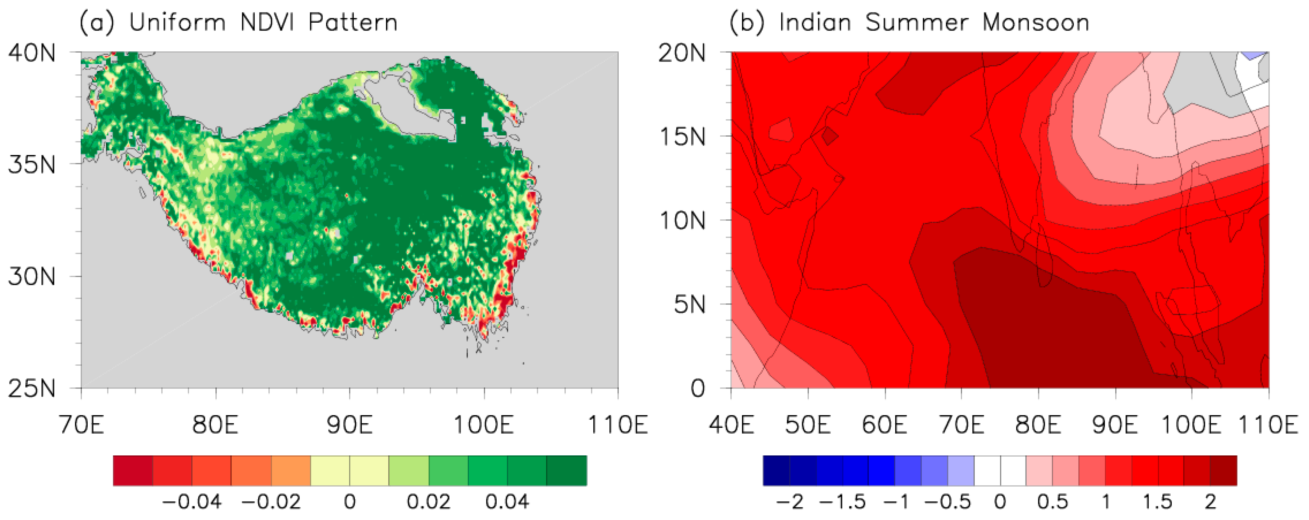
2.3.1. The Uniform NDVI Pattern and Its Index

We found two NDVI patterns dominating the TP in JJAS through the empirical orthogonal function (EOF) decomposition. The first dominant EOF mode features a uniform variation in NDVI anomalies on the TP, which is called the uniform NDVI pattern [35]. In this study, we used the REOF analysis to capture the prevalent and homogeneous patterns of the TP NDVI on inter-annual timescales, since the REOF analysis is more appropriate for the high-resolution and inhomogeneous distribution of the TP NDVI datasets.
The dominant modes obtained based on the EOF and REOF analyses highly resemble each other, and both show a uniform NDVI pattern. Moreover, their corresponding time series are significantly and positively linked. Their distinction is that the uniform pattern based on the REOF analysis does not show larger loadings on the southeast of the TP, which may be due to the high vegetation coverage and insignificant reactions to anomalous climate change over this region. Therefore, the first REOF mode of NDVI anomalies on the TP in JJAS from 1982 to 2020 is called the uniform NDVI pattern (Figure 2a), and its corresponding PC index is called the uniform NDVI pattern index (UNPI).

2.3.2. The Indian Summer Monsoon Index

In earlier studies, the Indian summer monsoon (ISM) index was defined as the all-Indian summer monsoon rainfall (AISMR) [71]. With the deepening of research, other indices representing the ISM were also proposed, such as the Webster–Yang index (WYI) [72], the monsoon Hadley circulation index (MHI) [73], the extended Indian monsoon rainfall index (EIMRI) [73], the Indian monsoon index (IMI) [74], and the Indian monsoon trough index (IMTI) [75]. Before exploring the influence of the ISM on the TP vegetation, the definitions and features of the abovementioned ISM indices were compared. Using the singular value decomposition and linear correlation, the WYI was most closely related to the uniform NDVI pattern (figures omitted). Therefore, following Webster and Yang [72], the area-mean vertical shear (U850-U200) of zonal winds over the region (40–110°E, 0–20°N) in June–August (JJA) was referred to as the ISM index (Figure 2b).

3. Results

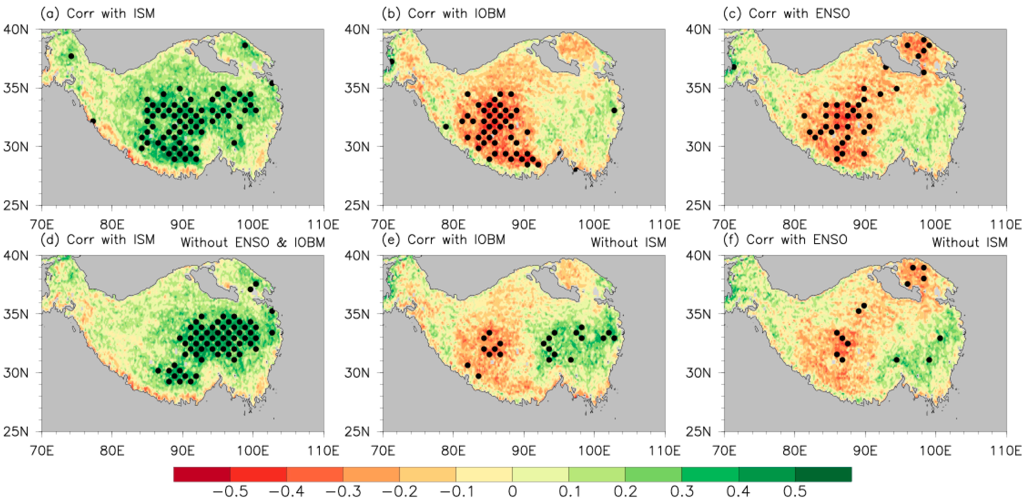
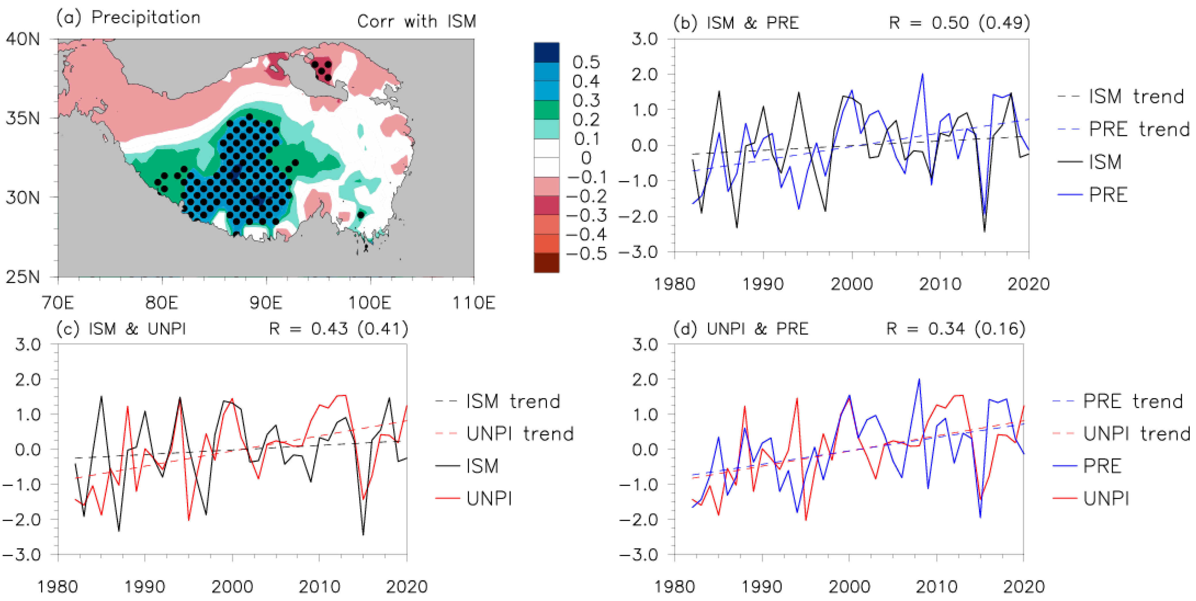
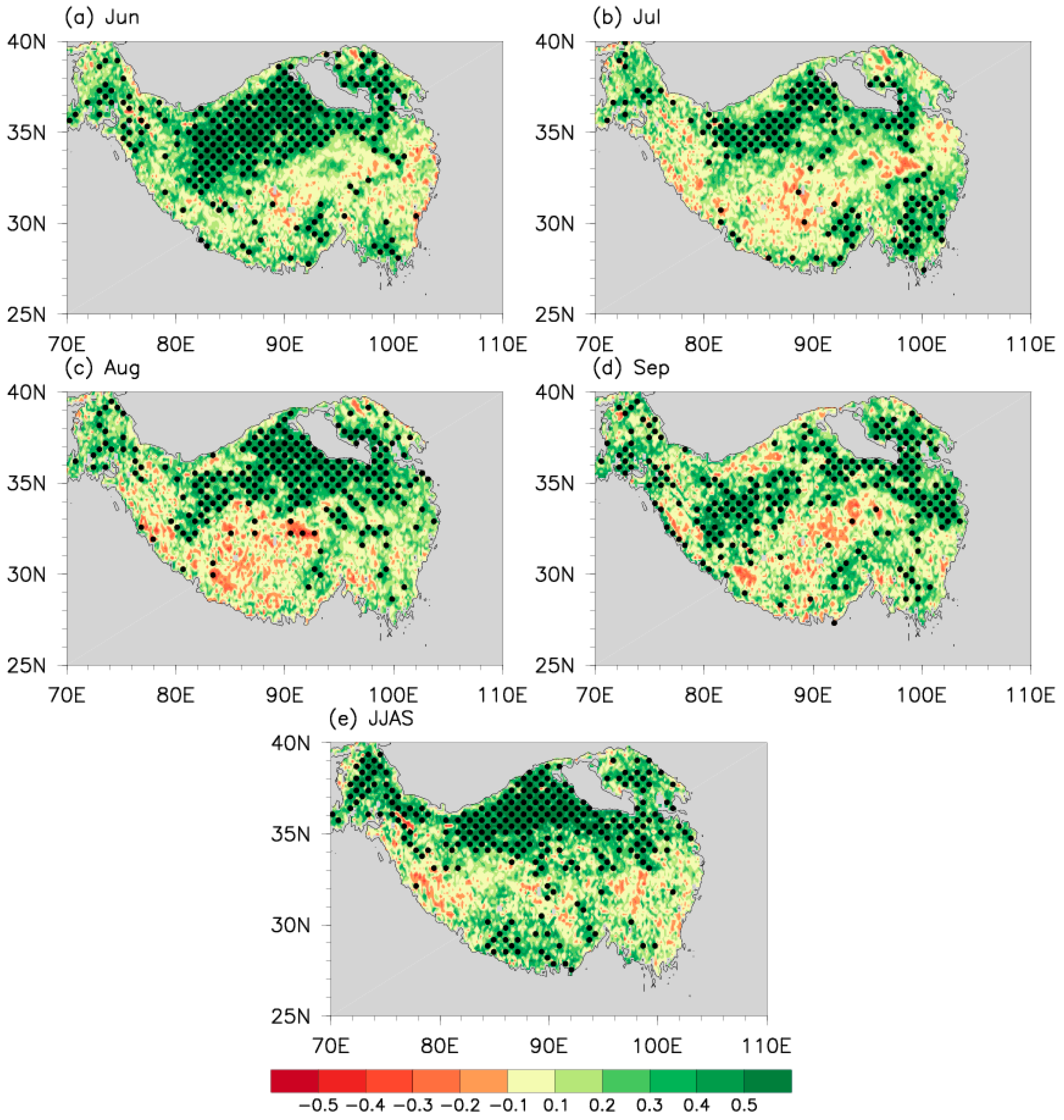
3.1. Correlations between the ISM and TP Precipitation and Vegetation

Precipitation is one of the main climatic factors affecting TP vegetation in the main growing season [35]. As mentioned in Section 1, the ISM is highly associated with TP precipitation. As such, the ISM should influence the inter-annual variability of vegetation on the TP by modulating precipitation over the TP. Moreover, the ENSO and IOBM can modulate the onset time and intensity of ISM [37,38,48,76,77]. This implies that the ENSO and IOBM may influence the TP precipitation by adjusting the ISM.
Figure 3 reveals the contribution of ENSO, IOBM, and ISM to the TP vegetation on inter-annual scales. A clear and significant positive correlation between the JJA ISM and JJAS TP NDVI appears over most of the TP, manifesting a similarly uniform NDVI pattern (Figure 3a). Moreover, the correlation coefficient between the UNPI and the ISM is 0.45, exceeding the confidence level of 99%. The JJAS TP NDVI is negatively correlated with the spring IBOM/previous winter ENSO, with large loadings (coefficients) roughly distributed on the southwestern TP/northeast–southwest oriented region (Figure 3b,c). These negative correlations reveal that corresponding to positive IOBM/El Niño, the ISM weakens [77]. The correlation coefficient between the UNPI and the spring IBOM is −0.25 and that between the UNPI and the previous winter ENSO is −0.26, which are lower than that between the UNPI and ISM (0.45). After removing the influence of the ISM via the partial correlation, the negative correlation between the spring IBOM (previous winter ENSO) and the JJAS TP NDVI significantly decreased (Figure 3e,f),and the coefficient dropped to −0.09 (−0.23) not reaching the 90% confidence level. To some extent, this implies that the ISM fulfills a “bridge” role linking the influence of ENSO and IOBM with the vegetation growth on the TP. The contribution of ENSO and IOBM to the TP vegetation becomes weaker due to the absence of the bridge effect of ISM.
In contrast, the correlation between the ISM and JJAS TP NDVI slightly decreases after removing the influence of ENSO and IOBM via the partial correlation, but a significantly positive correlation still covers the eastern TP (Figure 3d), showing a closer relationship than the ENSO-UNPI and IOBM-UNPI ones. After removing the influence of ENSO and IOBM, the correlation coefficient between the UNPI and ISM still reaches 0.29, significant at the 95% confidence level. This suggests that the ISM is not only a “bridge” relaying the influence of the ENSO and IOBM on the TP vegetation growth but also has a significant and direct effect on vegetation growth on the TP, albeit in the absence of ENSO and IOBM. Thus, we focus on the relationship between the ISM and the TP precipitation and NDVI in the following study.
Figure 4a presents the correlations of the ISM with the TP precipitation in May–August (MJJA). Note that the periods for the correlations are different from Figure 3c since precipitation has a one-month-lagged effect on the TP NDVI [24,25,29,35]. The ISM is highly positively linked with precipitation over the southwestern TP, exhibiting a central coefficient of 0.52, which reaches the confidence level of 95%. Based on the key region with significant correlations (Figure 4a), we referred to the area-mean precipitation anomaly over the southwest of the TP (80–92°E, 28–35°N) in MJJA as the precipitation index (PRE index). Time series of the ISM index, PRE index, and UNPI are compared in Figure 4b–d. In these figures, we can detect a slightly better correlation between the ISM and precipitation (0.50) than that between the ISM and NDVI (0.43), but both reach the confidence level of 99% (Figure 4b,c). Since precipitation directly affects the TP vegetation growth, the correlation between precipitation and the NDVI was expected to be greater than that between the ISM and NDVI. However, the former exceeds the 95% confidence level by 0.34 (Figure 4d), lower than the latter (Figure 4c). Note that all three indices exhibit a clear upward trend (Figure 4b–d); these correlations could be influenced by global warming. Therefore, their linear trends are removed in the subsequent sections.
After removing their linear trends, the ISM still maintains a significant correlation with the other two indices, which has an approximate coefficient of 0.49 (0.41) with the PRE index (UNPI) exceeding the confidence level of 99%. The PRE index mainly represents the ISM, exhibiting a regional correlation with precipitation over the TP (Figure 4a), while the UNPI represents the variation in vegetation on the overall TP. Thus, the PRE index’s correlation with the UNPI decreases from 0.34 to 0.16, which is significantly lower than the correlation between the ISM and UNPI (Figure 4c,d). Such a result implies that the influence of the ISM on the TP vegetation does not depend merely on precipitation, while other ISM-induced climatic factors may contribute to the TP vegetation growth. Clearly, the influence of the ISM on the TP vegetation requires further analysis.

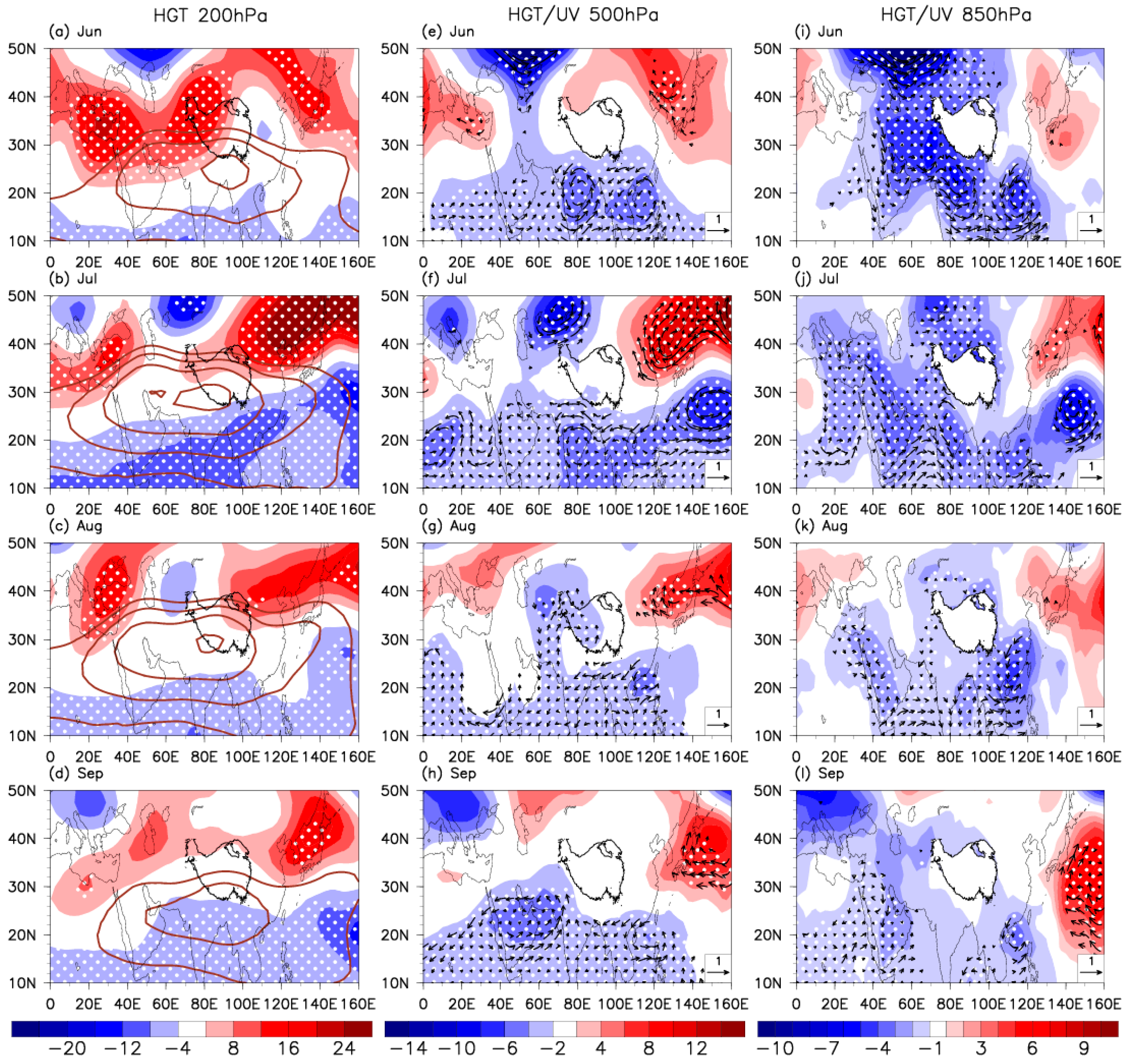
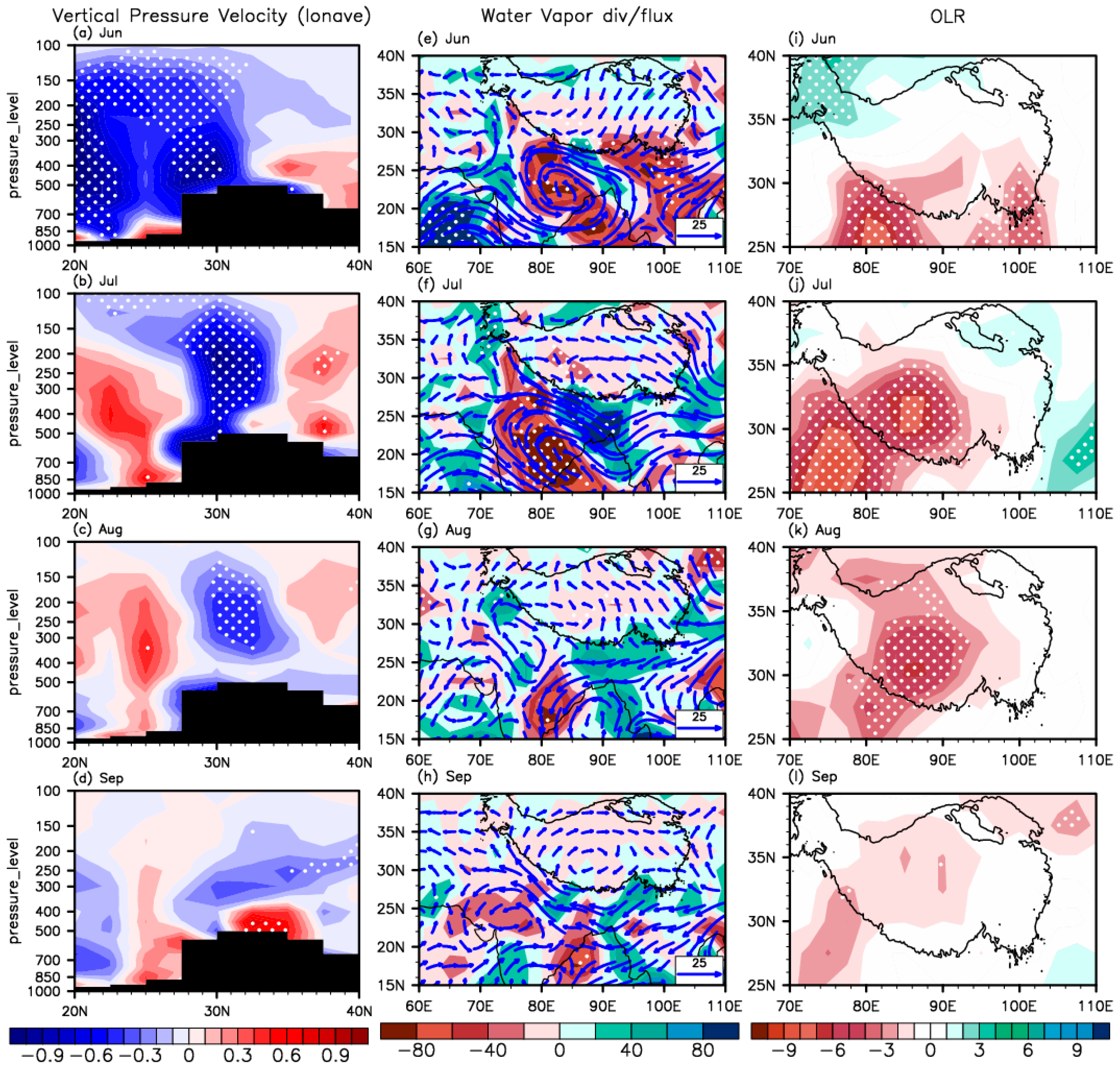
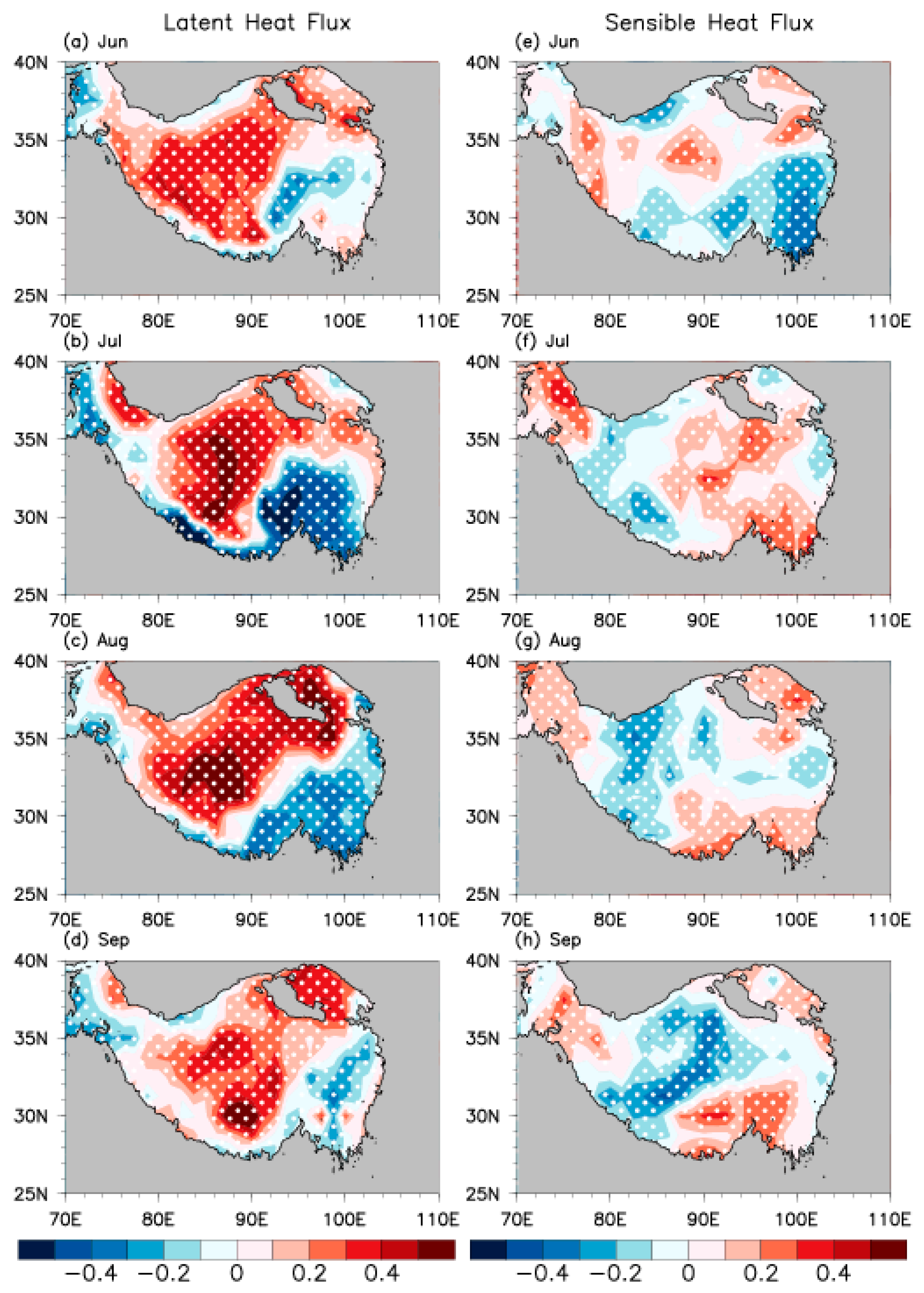
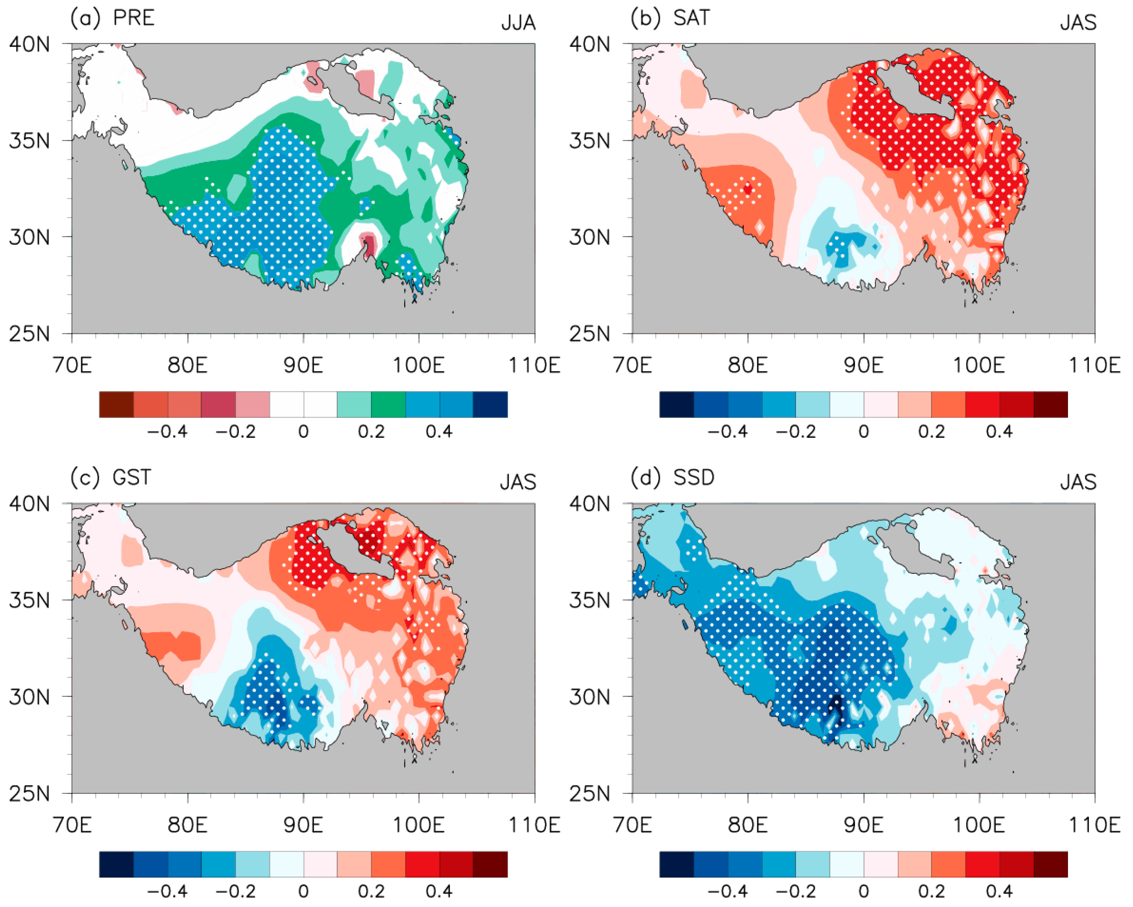
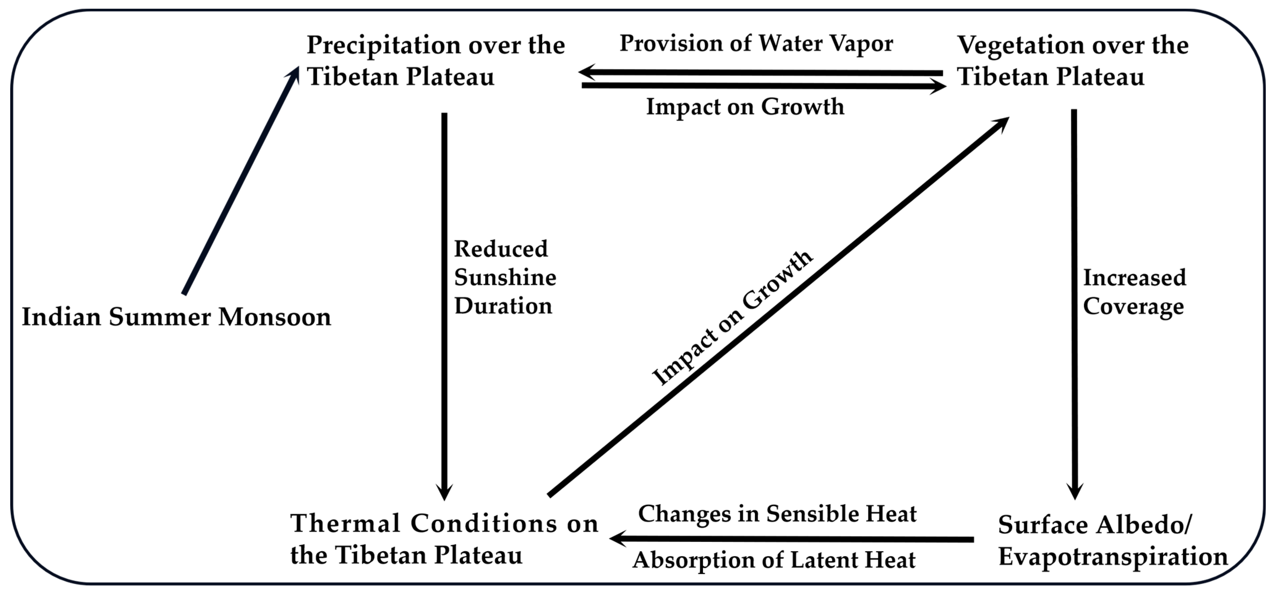
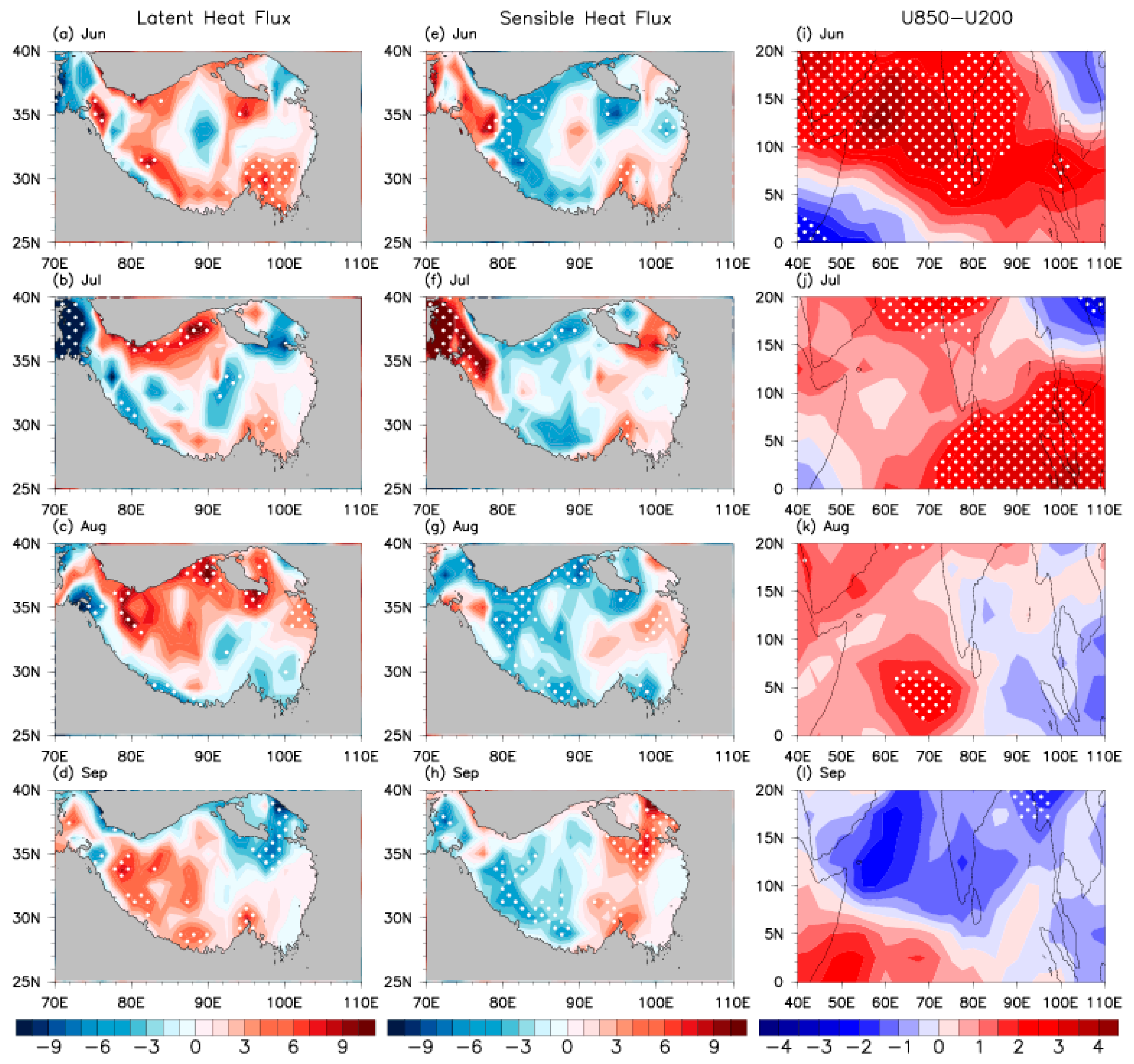
3.2. Physical Process of the ISM Affecting the TP Vegetation

As an external climatic factor, the ISM plays a role in modifying the vegetation growth on the TP NDVI by stimulating atmospheric circulation to alter the thermal and moisture conditions over the TP. In this section, the process of the ISM influencing the JJAS TP NDVI is explored by linear regression and partial correlation analyses in terms of the atmospheric circulation (Figure 5), water vapor transportation, convection (Figure 6), and thermal conditions over the TP (Figure 7).
In June, the climatological South Asia high (SAH) [78] in the upper troposphere (200 hPa) is situated south of 30°N, with its center around the southern TP. A strong positive geopotential height anomaly appears over the Iranian Plateau, indicating that the SAH significantly strengthens and shifts northwestward to the western TP (Figure 5a). In the middle-lower troposphere (500–850 hPa), two cyclonic convergences occur around the Indian and Indo-China Peninsulas where air pressure significantly decreases (Figure 5e,i). The enhanced SAH induces the ISM onset, which drives a significant increase in the transportation of water vapor from the Indian Ocean to the lower latitudes and accordingly facilitates water vapor converging over the southern TP (Figure 6e). The strengthened upward motion is induced by the low-pressure convergence and high-pressure divergence in the lower and upper troposphere, which occurs over the southern TP to the south of 30°N (Figure 6a). A negative outgoing longwave radiation (OLR) anomaly over the southern TP coincides with the entry of water vapor (Figure 6i).
By July, the location of the SAH in the upper troposphere essentially remains unmoved, but its area and intensity are significantly enhanced (Figure 5b). From June to July, the cyclonic convergence over the Indo-China Peninsula moves eastward to the northwest Pacific in the middle-lower troposphere. During the same period, the low pressure over the Indian Peninsula intensifies and slightly moves eastward (Figure 5f,j). Water vapor fluxes are shifted significantly northward, and then large quantities of water vapor are carried to the lower-latitude TP, where they then converge (Figure 6f). The enhanced upward motion over 25°–35°N and downward motion on either side (Figure 6b) promote convection, featuring a significant negative OLR anomaly over the southwestern TP (Figure 6j). This sufficient water vapor and strengthened convection contribute to the increase in precipitation.
As the SAH intensity decreases slightly in August (Figure 5c), the corresponding cyclonic convergences at 500 hPa and 850 hPa move westward to the Indo-China Peninsula, resulting in a weakening low pressure over the Bay of Bengal (Figure 5g,k). Changes in atmospheric circulation reduce the transportation of water vapor, which causes a consequent reduction in water vapor flux convergence to the southern TP (Figure 6g). The significant upward motion still appears over the overall TP (Figure 6c). Correspondingly, the negative OLR anomaly still appears over the central and western TP (Figure 6k), but the intensity begins to decrease, with the numerical value of the maximum OLR anomaly decreasing from approximately 9 W/m2 to 6 W/m2.
In September, the SAH intensity weakens substantially (Figure 5d), and a cyclonic circulation develops near the Arabian Sea in the mid-troposphere (Figure 5h). This causes the entire circulation system to move westward, with a significant downward motion (Figure 6d) and reduced convection (Figure 6l) over the TP.
As mentioned in Section 3.1, the ISM can influence vegetation on the TP through other climatic factors induced by the ISM besides precipitation, such as thermal factors (e.g., latent and sensible heat fluxes). Vegetation dynamics could largely affect the thermal conditions over the TP [12,13,14,15]. For example, the greening of TP vegetation can reduce surface albedo and thus increase sensible heat flux [14,15]. Based on that, we examined the partial correlation of the ISM with surface latent and sensible heat flux over the TP after removing the influence of the PRE index (Figure 7). Due to the annual cycle of vegetation growth on the TP, its coverage gradually increases from June to July. The consequently enhanced evapotranspiration of vegetation leads to substantial heat absorption, which promotes the transportation of latent heat across the TP and cools some regions of the TP. Meanwhile, the decrease in surface albedo induced by the substantial vegetation leads to an increase in sensible heat over most of the TP. Thus, the latent heat flux over the TP exhibits a distinct positive anomaly in JJA (Figure 7a,b), as does the sensible heat flux (Figure 7e,f). When the TP vegetation reaches its maximum coverage in August, the positive latent heat flux anomalies over the TP manifest the greatest magnitude, and the range of negative sensible heat anomalies also increases (Figure 7c,g). With the reduction in the TP vegetation in September, a significant decrease in the positive latent heat anomaly occurs over the TP, whereas the increased albedo leads to a wide range of negative sensible heat flux anomalies (Figure 7d,h).
Based on the above sections, we suggest the ISM may change air and ground temperature over the TP through varying vegetation growth. Additionally, the ISM-induced precipitation can affect the sunshine duration over the TP. Anomalous changes in these ISM-induced climatic factors jointly affect the NDVI inter-annual variability on the TP. Considering the one-month-lagged impact of precipitation on vegetation, the JJA precipitation anomaly, and the JAS surface air temperature, ground surface temperature and sunshine duration anomaly were regressed upon the ISM index (Figure 8).
Regulated by the ISM, precipitation increases significantly over the southwest of the TP and decreases over the Pamir Plateau and the southeast of the TP (Figure 8a). Surface air and ground temperatures exhibit significant warming over the northeastern TP to the north of 33°N (Figure 8b,c), which can contribute to higher NDVI across almost the entire TP. In fact, sunshine duration over the TP is not affected by the ISM, and the shorter sunshine duration should be attributed to the simultaneously increased precipitation. Precipitation increases abnormally over the southwest of the TP, where the sunshine duration is significantly shortened (Figure 8d). This finding is consistent with Mao et al. [35].
To examine the impact of the ISM-induced climatic factors on the NDVI inter-annual variability on the TP, we defined the corresponding indices in accordance with the significant regions (Figure 8) affected by these climatic factors. The JAS area-mean surface air temperature (ground surface temperature) anomalies over the north of the TP (70–104°E, 34–40°N) are referred to as the SAT (GST) index. The SSD index is determined in the same definition as the PRE index in Section 3.1, but in JAS. Based on the ISM and these indices, the following regression equation was established to estimate the UNPI.
U N P I e = 9.9   ×   10 9 0.15 P R E 0.39 S A T + 0.69 G S T 0.12 S S D + 0.28 I S M
in which the term on the left represents the estimate of UNPI (UNPIe), and the terms on the right represent the effect of these indices (PRE, SAT, GST, SSD and ISM) with different weights. For ease of calculation, the estimated intercept of 9.9 × 10⁻⁹ in Equation (1) is usually negligible.
Figure 9 presents the regression of the monthly NDVI anomaly upon the UNPIe in JJAS. Positive NDVI anomalies appear on the TP for each month (Figure 9a–d), displaying an approximately uniform NDVI pattern after four-month vegetation accumulation (Figure 9e). This suggests that the inter-annual variability of NDVI on the TP in JJAS can be attributed to the ISM and its induced changes in the local climatic factors in the TP, which can account for more than 52% of the variation in the UNPI.

4. Discussion

This paper indicates that the ISM is a significant external factor affecting the inter-annual variation in TP vegetation in the growing season, and examined the correlations among the ISM, the TP precipitation, and the TP vegetation. The findings reveal that the correlation between ISM and UNPI is much greater than that between UNPI and ISM-induced precipitation, especially when the linear trends of the three indices were removed (Figure 4b–d). The variations in the uniform NDVI pattern on the TP in JJAS on inter-annual scales are caused by a combination of several local climatic factors [35]. Therefore, instead of precipitation, other ISM-induced climatic factors dominate the inter-annual variations in vegetation on the TP. In addition to regulating the atmospheric circulation and associated precipitation over the TP, the ISM can also influence the inter-annual variability of vegetation by inducing changes in the TP thermal conditions. Figure 10 summarizes the process of the ISM influencing the vegetation growth on the TP.
In the main growing season (JJAS), changes in the SAH concerning its location and intensity cause higher pressure (positive HGT anomalies) over the TP in the upper troposphere, and lower pressure (negative HGT anomalies) at the lower-latitude TP in the middle-lower troposphere (Figure 5). Such an atmospheric circulation structure, with atmospheric divergence and convergence in the upper and middle-lower troposphere, respectively, enhances the upward motion over the TP (Figure 6a–d). Furthermore, the transport of water vapor through the Indian Ocean entering the lower-latitude TP is facilitated by the strengthened cyclone activity in the lower troposphere (Figure 6e–h). The sufficient water vapor and strengthened convection can increase precipitation over the TP, thus promoting vegetation growth.
Vegetation evapotranspiration modulates thermal conditions over the TP as a result of the physical phase transition of water, as well as altering the local atmospheric water vapor content and associated precipitation. Additionally, the variations in vegetation coverage also can affect surface sensible heat flux by modifying the TP surface elements, such as albedo and roughness. With the gradual increase in vegetation, the enhanced evapotranspiration replenishes the atmospheric water vapor over the TP while absorbing latent heat (Figure 7a–d) and altering surface sensible heat (Figure 7e–h). Due to the interaction between vegetation and temperature, a certain degree of warming promotes vegetation growth. According to earlier studies, changes in thermal conditions over the TP may also affect vegetation growth [23,24,25,26], and moderate warming of the northern TP effectively promotes the growth of local vegetation [35]. Additionally, the ISM-induced increase in precipitation can also lead to the lack of sunshine, which interferes with vegetation growth on the TP [25].
We further explored the joint effects of the ISM and its induced changes in local climatic factors (precipitation, air temperature, ground temperature, sunshine duration, etc.) on the uniform NDVI pattern using multiple regression (Equation (1)). These factors jointly modulate more than 52% of the variation in the UNPI. In other words, the ISM not only influences the TP vegetation growth through precipitation, but also can regulate the TP vegetation growth through modulating the variations in thermal factors in the TP. The current findings are based on statistical analyses, which are insufficient to clarify the influence of the ISM on the TP vegetation. We will further verify the results through numerical experiments in the future.
Various factors have an impact on the ISM, such as the TP diabatic heating, land–sea thermal contrast, ENSO, and internal atmospheric processes [37,47,48,49,53]. Among these factors, the TP atmospheric heat source directly affects the ISM onset, and its diabatic heating also plays a decisive role in the intensity and location of the ISM [52,53]. Additionally, the increased vegetation on the TP can cause changes in local thermal conditions (Figure 7). This raises an interesting question, that is, can the TP vegetation regulate the ISM through the alteration of TP thermal conditions in its main growing season?
Table 1 exhibits the correlation coefficients between the monthly ISM from June to September and the one-month-lagged, simultaneous, and summer (JAS) UNPIs. The ISM and the one-month-lagged (summer) UNPI are positively correlated, with the highest association between the July ISM and August (summer) UNPI. The finding indicates the response of the TP NDVI to the influence of the ISM in its main growing season. The ISM is closely correlated with the simultaneous UNPI in June–July. However, the correlation between the ISM and the simultaneous UNPI is insignificant in August–September. These imply the possible influence of the UNPI on the ISM. The September ISM is hardly relevant with summer UNPI with a coefficient of only −0.03, which suggests the ISM-UNPI correlation has vanished at this time.
The differences in latent and sensible heat fluxes over the TP, and the vertical shear of zonal winds over the region (40–110°E, 0–20°N), are analyzed for typical positive and negative UNPI years (Figure 11), where the changes in the ISM intensity can reflect the correlation between the ISM and UNPI. The typical UNPI years are characterized as having an absolute value of the UNPI larger than a threshold of 0.5 standard deviations (see Table 2). In June–July, the substantial growth and increased coverage of the TP vegetation result in enhanced evapotranspiration and transportation of latent heat (positive anomalies) over the central and northern TP (Figure 11a,b). A clear decrease in sensible heat fluxes (negative anomalies) appears there, while the sensible heat fluxes increase significantly over the northwest corner and southeast of the TP due to the reduced surface albedo (Figure 11e,f). During this period, the relationship between the ISM and UNPI gradually becomes stronger (Figure 11i,j). When the NDVI reaches its maximum coverage in August, positive latent heat flux anomalies keep increasing due to the vegetation evapotranspiration (Figure 11c), and the magnitude of negative sensible heat flux anomalies increases throughout the whole TP except for the southeast (Figure 11g). In contrast, there is no significant increase in the sensible heat fluxes over the southeastern TP because the vegetation coverage (albedo) no longer increases (decreases) (Figure 11g). The overall TP exhibits cooling, while the correlation between the UNPI and ISM is somewhat weakened (Figure 11k). In September, the vegetation still shows strong overall evapotranspiration over the TP despite the decrease in TP vegetation coverage. Most of the TP experiences significantly increased latent heat flux (Figure 11d), and the western TP to the west of 90°E experiences a significant decrease in sensible heat flux (Figure 11h). Meanwhile, the ISM-UNPI correlation seems to disappear (Figure 11l).
Comparing Table 1 and Figure 11, we speculate that the influence of the NDVI on the TP thermal conditions could play a de-correlation role between the ISM and the TP vegetation in late summer and early autumn. However, our current findings are insufficient to confirm the above opinion. The specific physical mechanism requires further study. The current findings reveal a closer relationship of the TP vegetation with the ISM than that with the IOBM and ENSO on inter-annual scales, explore the influence of the ISM on the TP vegetation, and preliminarily present the speculation of the potential physical process. However, as a “bridge” linking the potential contributions of ENSO and IOBM with vegetation growth on the TP, the effect of the ISM on the growth of the TP vegetation needs to be further quantified. Therefore, a series of numerical experiments should be performed in the future to quantify the specific contributions of several external climatic factors (e.g., the ISM, IOBM, ENSO) to the inter-annual variability of the TP NDVI, especially the role of the ISM. These studies may further deepen our understanding of the relationship between the TP vegetation and regional and global climate change and facilitate future predictions of vegetation activity on the TP on inter-annual scales.

5. Conclusions

Using remote-sensing-based NDVI, several sets of reanalysis, and meteorological station observed data, this paper explored the influence of the ISM on the NDVI inter-annual variability on the TP in JJAS. The findings reveal that the ISM is an external factor affecting the inter-annual variation of TP vegetation in the growing season. Furthermore, the contribution of ISM is more direct and significant than that of ENSO and IOBM. The ISM, TP NDVI, and TP precipitation are all positively correlated with each other. Although precipitation is a direct factor of vegetation growth, the correlation between precipitation and NDVI greatly decreases after removing their linear trends and is much smaller than that between the ISM and NDVI. This implies that the ISM influences the TP vegetation not only by changing precipitation but also by inducing the changes in thermal factors in the TP.
Corresponding to a strong ISM, anticyclonic circulation develops over the TP in the upper troposphere, and significant cyclonic circulation develops over the southern TP in the middle-lower troposphere, which also represents a strengthened SAH. This upper and middle-lower tropospheric circulation structure enhances upward motion over the TP. Moreover, the middle-lower tropospheric cyclones can induce more water vapor to the south of the TP. The sufficient water vapor and strengthened upward motion both facilitate more precipitation over the southwest of the TP, which affects vegetation growth. The ISM-induced increase in precipitation over the TP also affects the TP thermal conditions by modulating sunshine duration. Moreover, vegetation can affect TP thermal conditions through its evapotranspiration and coverage. The increased vegetation causes the TP warming, and the TP warming can in turn promote vegetation growth. Further multiple regression analysis revealed that the ISM and its induced changes in local climatic factors can account for more than 52% of the NDVI inter-annual variability on the TP in JJAS.
Additionally, changes in TP thermal conditions, which are regulated by the NDVI in late summer and early autumn, may influence the relationship between the ISM and TP vegetation. In the early growing season (June–July), the UNPI and ISM are significantly correlated. Composite analysis suggests that the TP NDVI causes the changes in TP thermal conditions and thus affects the ISM intensity. Relative to June–July, the ISM intensity is weaker in August–September. This weakening will be more severe in the case of increased vegetation, which may disturb and weaken the correlation between the ISM and TP vegetation in late summer and early autumn.

Author Contributions

Conceptualization, H.-L.R.; methodology, H.-L.R. and G.L.; formal analysis, X.M.; data curation, X.M.; writing—original draft preparation, X.M., H.-L.R. and G.L.; writing—review and editing, X.M., H.-L.R. and G.L.; funding acquisition, B.S. and Y.S. All authors edited the manuscript. All authors have read and agreed to the published version of the manuscript.

Funding

The National Key R&D Program of China (Grant 2022YFF0801603), the Second Tibetan Plateau Scientific Expedition and Research (STEP) program (Grant 2019QZKK0105), the Strategic Priority Research Program of the Chinese Academy of Sciences (Grant XDA2010030807), and the Basic Research Fund of CAMS (Grant 2021Z007) all provided financial support for this study.

Data Availability Statement

ECOCAST supplied the GIMMS NDVI3g data for this study, which can be obtained from the website at https://ecocast.arc.nasa.gov/data/pub/gimms/ (accessed on 29 November 2020). LAADS DAAC/NASA made the MCD19A3CMG data available on the website at https://ladsweb.modaps.eosdis.nasa.gov/ (accessed on 6 July 2023). The National Meteorological Information Center supplied the daily meteorological dataset of basic meteorological elements of China National Surface Weather Station (V3.0) on the website at http://data.cma.cn/ (accessed on 30 December 2021). The ERA5 reanalysis datasets were publicly available at https://cds.climate.copernicus.eu/cdsapp#!/home/ (accessed on 21 October 2021). The NOAA PSL, Boulder, Colorado, USA, supplied the outgoing longwave radiation (OLR) data from their website at https://psl.noaa.gov (accessed on 21 October 2021). The JRA-55 dataset was publicly available at https://rda.ucar.edu/datasets/ds628.1/ (accessed on 5 October 2022). The Niño 3.4 index was publicly available at https://psl.noaa.gov/data/correlation/nina34.anom.data (accessed on 1 May 2023). The IOBM index was publicly available at http://cmdp.ncc-cma.net/Monitoring/cn_nino_index.php?product=cn_nino_index_iobw (accessed on 1 May 2023).

Acknowledgments

We are grateful to LAADS DAAC/NASA and ECOCAST for supplying the remote sensing datasets. We thank National Meteorological Information Center for supplying all daily station-observed datasets. We thank NOAA PSL for providing the NOAA Interpolated Outgoing Longwave Radiation (OLR) dataset. We thank ECMWF and NCAR UCAR for providing data. We thank NOAA CPC for providing the Niño 3.4 index and NCC/CMA for providing the IOBM index.

Conflicts of Interest

The authors declare no conflict of interest.

References

  1. Ye, D.Z. Some characteristics of the summer circulation over the Qinghai-Xizang (Tibet) Plateau and its neighborhood. Bull. Amer. Meteorl. Soc. 1981, 62, 14–19. [Google Scholar] [CrossRef]
  2. Ye, D.Z.; Wu, G.X. The role of the heat source of the Tibetan Plateau in the general circulation. Meteorol. Atmos.Phys. 1998, 67, 181–198. [Google Scholar] [CrossRef]
  3. Liu, G.; Zhao, P.; Chen, J. Possible effect of the thermal condition of the Tibetan Plateau on the interannual variability of the summer Asian-Pacific oscillation. J. Clim. 2017, 30, 9965–19977. [Google Scholar] [CrossRef]
  4. Liu, Y.M.; Lu, M.M.; Yang, H.J.; Duan, A.M.; He, B.; Yang, S.; Wu, G.X. Land–atmosphere–ocean coupling associated with the Tibetan Plateau and its climate impacts. Natl. Sci. Rev. 2020, 7, 534–552. [Google Scholar] [CrossRef]
  5. Jiang, X.; Li, Y.; Yang, S.; Yang, K.; Chen, J. Interannual Variation of Summer Atmospheric Heat Source over the Tibetan Plateau and the Role of Convection around the Western Maritime Continent. J. Clim. 2016, 29, 121–138. [Google Scholar] [CrossRef]
  6. Wu, Z.W.; Zhang, P.; Chen, H.; Li, Y. Can the Tibetan Plateau snow cover influence the interannual variations of Eurasian heat wave frequency? Clim. Dyn. 2015, 46, 3405–3417. [Google Scholar] [CrossRef]
  7. Xu, X.D.; Zhao, T.L.; Shi, X.H.; Lu, C.G. A study of the role of the Tibetan Plateau′s thermal forcing in modulating rainband and moisture transport in eastern China. Acta Meteorol. Sin. 2015, 73, 20–35. (In Chinese) [Google Scholar] [CrossRef]
  8. Wu, G.X.; Liu, Y.M.; He, B.; Bao, Q.; Wang, Z.Q. Review of the impact of the Tibetan Plateau sensible heat driven air-pump on the Asian summer monsoon. Chin. J. Atmos. Sci. 2018, 42, 488–504. [Google Scholar] [CrossRef]
  9. Cai, Y.; Han, X.; Zhao, H.; Klotzbach, P.J.; Wu, L.; Raga, G.B.; Wang, C. Enhanced Predictability of Rapidly Intensifying Tropical Cyclones over the Western North Pacific Associated with Snow Depth Changes over the Tibetan Plateau. J. Clim. 2022, 35, 2093–2110. [Google Scholar] [CrossRef]
  10. Chen, B.X.; Zhang, X.Z.; Tao, J.; Wu, J.S.; Wang, J.S.; Shi, P.L.; Zhang, Y.J.; Yu, C.Q. The impact of climate change and anthropogenic activities on alpine grassland over the Qinghai-Tibet Plateau. Agric. For. Meteorol. 2014, 189–190, 11–18. [Google Scholar] [CrossRef]
  11. Wang, Z.; Niu, B.; He, Y.; Zhang, J.; Wu, J.; Wang, X.; Zhang, Y.; Zhang, X. Weakening summer westerly circulation actuates greening of the Tibetan Plateau. Glob. Planet. Chang. 2022, 221, 104027. [Google Scholar] [CrossRef]
  12. Yang, K.; Ye, B.S.; Zhou, D.G.; Wu, B.Y.; Foken, T.; Qin, J.; Zhou, Z.Y. Response of hydrological cycle to recent climate changes in the Tibetan Plateau. Clim. Chang. 2011, 109, 517–534. [Google Scholar] [CrossRef]
  13. Piao, S.; Tan, K.; Nan, H.; Ciais, P.; Fang, J.; Wang, T.; Vuichard, N.; Zhu, B. Impacts of climate and CO2 changes on the vegetation growth and carbon balance of Qinghai–Tibetan grasslands over the past five decades. Glob. Planet. Chang. 2012, 98–99, 73–80. [Google Scholar] [CrossRef]
  14. Fan, G.Z.; Chen, G.D. Interactions between Physiological Process of the Tibetan Plateau Vegetation and CO2 Concentration and Climate Change. Chin. J. Atmos. Sci. 2002, 26, 509–518. [Google Scholar] [CrossRef]
  15. Shen, M.G.; Piao, S.L.; Jeong, S.J.; Zhou, L.M.; Zeng, Z.Z.; Ciais, P.; Chen, D.L.; Huang, M.T.; Jin, C.S.; Li, L.; et al. Evaporative cooling over the Tibetan Plateau induced by vegetation growth. Proc. Natl. Acad. Sci. USA 2015, 112, 9299–9304. [Google Scholar] [CrossRef]
  16. Kumari, N.; Saco, P.M.; Rodriguez, J.F.; Johnstone, S.A.; Srivastava, A.; Chun, K.P.; Yetemen, O. The grass is not always greener on the other side: Seasonal reversal of vegetation greenness in aspect-driven semiarid ecosystems. Geophys. Res. Lett. 2020, 47, e2020GL088918. [Google Scholar] [CrossRef]
  17. Rouse, J.W.; Haas, R.H.; Schell, J.A.; Deering, D.W. Monitoring the Vernal Advancement and Retrogradation (Green Wave Effect) of Natural Vegetation. Contractor Report; 1973. Available online: https://ntrs.nasa.gov/citations/19750020419 (accessed on 8 July 2023).
  18. Huete, A.; Didan, K.; Miura, T.; Rodriguez, E.P.; Gao, X.; Ferreira, L.G. Overview of the radiometric and biophysical performance of the MODIS vegetation indices. Remote Sens. Environ. 2002, 83, 195–213. [Google Scholar] [CrossRef]
  19. Justice, C.O.; Wharton, S.W.; Holben, B.N. Application of digital terrain data to quantify and reduce the topographic effect on Landsat data. Int. J. Remote Sens. 1981, 2, 213–230. [Google Scholar] [CrossRef] [Green Version]
  20. Martín-Ortega, P.; García-Montero, L.G.; Sibelet, N. Temporal patterns in illumination conditions and its effect on vegetation indices using Landsat on Google Earth Engine. Remote Sens. 2020, 12, 211. [Google Scholar] [CrossRef] [Green Version]
  21. Matsushita, B.; Yang, W.; Chen, J.; Onda, Y.; Qiu, G. Sensitivity of the enhanced vegetation index (EVI) and normalized difference vegetation index (NDVI) to topographic effects: A case study in high-density cypress forest. Sensors 2007, 7, 2636–2651. [Google Scholar] [CrossRef] [Green Version]
  22. Huang, K.; Zhang, Y.; Zhu, J.; Liu, Y.; Zu, J.; Zhang, J. The Influences of Climate Change and Human Activities on Vegetation Dynamics in the Qinghai-Tibet Plateau. Remote Sens. 2016, 8, 876. [Google Scholar] [CrossRef] [Green Version]
  23. Piao, S.; Mohammat, A.; Fang, J.; Qiang, C.; Feng, J. NDVI- based increase in growth of temperate grasslands and its responses to climate changes in China. Glob. Environ. Chang. 2006, 16, 340–348. [Google Scholar] [CrossRef]
  24. Cao, X.J.; Ganjurjav, H.; Liang, Y.; Gao, Q.Z.; Zhang, Y.; Li, Y.E.; Wan, Y.F.; Danjiu, L.B. Temporal and spatial distribution of grassland degradation in northern Tibet based on NDVI. Acta Pratacult. Sin. 2016, 25, 1–8. (In Chinese) [Google Scholar] [CrossRef]
  25. Du, J.Q.; Zhao, C.X.; Shu, J.M.; Jiaerheng, A.; Yuan, X.J.; Yin, J.Q.; Fang, S.F.; He, P. Spatiotemporal changes of vegetation on the Tibetan Plateau and relationship to climatic variables during multiyear periods from 1982–2012. Environ. Earth Sci. 2016, 75, 77. [Google Scholar] [CrossRef]
  26. Li, W.X.; Xu, J.; Yao, Y.Q.; Zhang, Z.C. Temporal and Spatial Changes in the Vegetation Cover (NDVI) in the Three-River Headwater Region, Tibetan Plateau, China under Global Warming. Mt. Res. 2021, 39, 473–482. (In Chinese) [Google Scholar] [CrossRef]
  27. Chai, L.F.; Tian, L.; Ao, Y.; Wang, X.Q. Influence of Human Disturbance on the Change of Vegetation Cover in the Tibetan Plateau. Res. Soil Water Conserv. 2021, 28, 382–388. [Google Scholar]
  28. Liu, S.; Zhang, Y.; Cheng, F.; Hou, X.; Zhao, S. Response of Grassland Degradation to Drought at Different Time-Scales in Qinghai Province: Spatio-Temporal Characteristics, Correlation, and Implications. Remote Sens. 2017, 9, 1329. [Google Scholar] [CrossRef] [Green Version]
  29. Ding, M.J.; Zhang, Y.L.; Liu, L.S.; Wang, Z.F. Temporal and spatial distribution of grassland coverage change in Tibetan Plateau since 1982. J. Nat. Resour. 2010, 25, 2114–2122. [Google Scholar] [CrossRef]
  30. Salzer, M.W.; Larson, E.R.; Bunn, A.G.; Hughes, M.K. Changing climate response in near-treeline bristlecone pine with elevation and aspect. Environ. Res. Lett. 2014, 9, 114007. [Google Scholar] [CrossRef]
  31. Zhang, B.; Zhang, Y.; Wang, Z.; Ding, M.; Liu, L.; Li, L.; Li, S.; Liu, Q.; Paudel, B.; Zhang, H. Factors Driving Changes in Vegetation in Mt. Qomolangma (Everest): Implications for the Management of Protected Areas. Remote Sens. 2021, 13, 4725. [Google Scholar] [CrossRef]
  32. Weltzin, J.F.; Loik, M.E.; Schwinning, S.; Williams, D.G.; Fay, P.A.; Haddad, B.M.; Harte, J.; Huxman, T.E.; Knapp, A.K.; Lin, G.; et al. Assessing the response of terrestrial ecosystems to potential changes in precipitation. BioScience 2003, 53, 941–952. [Google Scholar] [CrossRef]
  33. Sarkar, S.; Kafatos, M. Interannual variability of vegetation over the Indian sub-continent and its relation to the different meteorological parameters. Remote Sens. Environ. 2004, 90, 268–280. [Google Scholar] [CrossRef]
  34. Yu, M.; Wang, G.L.; Parr, D.; Ahmed, K.F. Future changes of the terrestrial ecosystem based on a dynamic vegetation model driven with RCP8.5 climate projections from 19 GCMs. Clim. Chang. 2014, 127, 257–271. [Google Scholar] [CrossRef]
  35. Mao, X.; Ren, H.-L.; Liu, G. Primary Interannual Variability Patterns of the Growing-Season NDVI over the Tibetan Plateau and Main Climatic Factors. Remote Sens. 2022, 14, 5183. [Google Scholar] [CrossRef]
  36. Wu, G.X.; Duan, A.M.; Liu, Y.M.; Yan, J.H.; Liu, B.Q.; Ren, S.L.; Zhang, H.Y.; Wang, T.M.; Liang, X.Y.; Guan, Y. Recent Advances in the Study on the Dynamics of the Asian Summer Monsoon Onset. Chin. J. Atmos. Sci. 2013, 37, 211–228. [Google Scholar] [CrossRef]
  37. Dong, W.; Lin, Y.; Wright, J.S.; Ming, Y.; Xie, Y.; Wang, B.; Luo, Y.; Huang, W.; Huang, J.; Wang, L.; et al. Summer rainfall over the southwestern Tibetan Plateau controlled by deep convection over the Indian subcontinent. Nat. Commun. 2016, 7, 10925. [Google Scholar] [CrossRef] [Green Version]
  38. Jiang, X.W.; Ting, M. A Dipole Pattern of Summertime Rainfall across the Indian Subcontinent and the Tibetan Plateau. J. Clim. 2017, 30, 9607–9620. [Google Scholar] [CrossRef]
  39. Liu, X.; Yin, Z.-Y. Spatial and temporal variation of summer precipitation over the eastern Tibetan Plateau and the North Atlantic Oscillation. J. Clim. 2001, 14, 2896–2909. [Google Scholar] [CrossRef]
  40. Wang, Z.Q.; Yang, S.; Lau, N.C.; Duan, A.M. Teleconnection between summer NAO and East China rainfall variations: A bridge effect of the Tibetan Plateau. J. Clim. 2018, 31, 6433–6444. [Google Scholar] [CrossRef]
  41. Hu, S.; Zhou, T.; Wu, B. Impact of Developing ENSO on Tibetan Plateau Summer Rainfall. J. Clim. 2021, 34, 3385–3400. [Google Scholar] [CrossRef]
  42. Chen, X.Y.; You, Q.L. Effect of Indian Ocean SST on Tibetan Plateau precipitation in the early rainy season. J. Clim. 2017, 30, 8973–8985. [Google Scholar] [CrossRef]
  43. Gao, Y.; Wang, H.; Li, S. Influences of the Atlantic Ocean on the summer precipitation of the southeastern Tibetan Plateau. J. Geophys. Res. Atmos. 2013, 118, 3534–3544. [Google Scholar] [CrossRef]
  44. Jiang, X.W.; Zhang, T.T.; Tam, C.Y.; Chen, J.W.; Lau, N.C.; Yang, S.; Wang, Z.Y. Impacts of ENSO and IOD on Snow Depth Over the Tibetan Plateau: Roles of Convections Over the Western North Pacific and Indian Ocean. J. Geophys. Res. Atmos. 2019, 124, 11961–11975. [Google Scholar] [CrossRef]
  45. He, K.; Liu, G.; Zhao, J.; Li, J. Co-variability of the summer NDVIs on the eastern Tibetan Plateau and in the Lake Baikal region: Associated climate factors and atmospheric circulation. PLoS ONE 2020, 15, e0239465. [Google Scholar] [CrossRef]
  46. Wang, H.; Liu, G.; Wang, S.; He, K. Precursory Signals (SST and Soil Moisture) of Summer Surface Temperature Anomalies over the Tibetan Plateau. Atmosphere 2021, 12, 146. [Google Scholar] [CrossRef]
  47. Chen, G.; Huang, R. Excitation Mechanisms of the Teleconnection Patterns Affecting the July Precipitation in Northwest China. J. Clim. 2012, 25, 7834–7851. [Google Scholar] [CrossRef]
  48. Feng, L.; Zhou, T. Water vapor transport for summer precipitation over the Tibetan Plateau: Multidata set analysis. J. Geophys. Res. Atmos. 2012, 117, 85–99. [Google Scholar] [CrossRef] [Green Version]
  49. Yao, T.; Masson-Delmotte, V.; Gao, J.; Yu, W.S.; Yang, X.X.; Risi, C.; Sturm, C.; Werner, M.; Zhao, H.B.; He, Y.; et al. A review of climatic controls on δ18O in precipitation over the Tibetan Plateau: Observations and simulations. Rev. Geophys. 2013, 51, 525–548. [Google Scholar] [CrossRef]
  50. Wei, W.; Ren, Q.; Lu, M.; Yang, S. Zonal Extension of the Middle East Jet Stream and Its Influence on the Asian Monsoon. J. Clim. 2022, 35, 4741–4751. [Google Scholar] [CrossRef]
  51. Yanai, M.; Li, C.F.; Song, Z.S. Seasonal heating of the plateau and its effects on the evolution of the Asian monsoon. J. Meteor. Soc. Jpn. 1992, 70, 319–351. [Google Scholar] [CrossRef] [Green Version]
  52. Ting, M.F. Maintenance of Northern Summer Stationary Waves in a GCM. J. Atmos. Sci. 1994, 51, 3286–3308. [Google Scholar] [CrossRef]
  53. Wu, G.X.; Zhang, Y. Tibetan Plateau Forcing and the Timing of the Monsoon Onset over South Asia and the South China Sea. Mon. Weather Rev. 1998, 126, 913–927. [Google Scholar] [CrossRef]
  54. Wu, R. A mid-latitude Asian circulation anomaly pattern in boreal summer and its connection with the Indian and East Asian summer monsoons. Int. J. Climatol. 2002, 22, 1879–1895. [Google Scholar] [CrossRef]
  55. Fensholt, R.; Rasmussen, K.; Nielsen, T.T.; Mbow, C. Evaluation of earth observation based long term vegetation trends—Intercomparing NDVI time series trend analysis consistency of Sahel from AVHRR GIMMS, Terra MODIS and SPOT VGT data. Remote Sens. Environ. 2009, 113, 1886–1898. [Google Scholar] [CrossRef]
  56. Alcaraz-Segura, D.; Liras, E.; Tabik, S.; Paruelo, J.; Cabello, J. Evaluating the consistency of the 1982–1999 NDVI trends in the Iberian Peninsula across four time-series derived from the AVHRR sensor. LTDR, GIMMS, FASIR, and PAL-II. Sensors 2010, 10, 1291–1314. [Google Scholar] [CrossRef]
  57. Fensholt, R.; Rasmussen, K. Analysis of trends in the Sahelian ‘rain-use efficiency’ using GIMMS NDVI, RFE and GPCP rainfall data. Remote Sens. Environ. 2011, 115, 438–451. [Google Scholar] [CrossRef]
  58. Lyapustin, A.; Wang, Y.; Laszlo, I.; Korkin, S. Improved cloud and snow screening in MAIAC aerosol retrievals using spectral and spatial analysis, Atmos. Meas. Tech. 2012, 5, 843–850. [Google Scholar] [CrossRef] [Green Version]
  59. Lyapustin, A.; Wang, Y.; Korkin, S.; Huang, D. MODIS Collection 6 MAIAC Algorithm. Atmos. Meas. Tech. 2018, 11, 5741–5765. [Google Scholar] [CrossRef] [Green Version]
  60. Gallo, K.; Li, J.; Reed, B.; Eidenshink, J.; Dwyer, J. Multi-platform comparisons of MODIS and AVHRR normalized difference vegetation index data. Remote Sens. Environ. 2005, 99, 221–231. [Google Scholar] [CrossRef] [Green Version]
  61. Fensholt, R.; Proud, S.R. Evaluation of Earth Observation based global long term vegetation trends—Comparing GIMMS and MODIS global NDVI time series. Remote Sens. Environ. 2012, 119, 131–147. [Google Scholar] [CrossRef]
  62. Du, J.Q.; Shu, J.M.; Wang, Y.H.; Li, Y.C.; Zhang, L.B.; Guo, Y. Comparison of GIMMS and MODIS normalized vegetation index composite data for Qinghai-Tibet Plateau. Chin. J. Appl. Ecol. 2015, 25, 533–544. (In Chinese) [Google Scholar]
  63. Hersbach, H.; Bell, B.; Berrisford, P.; Biavati, G.; Horányi, A.; Muñoz Sabater, J.; Nicolas, J.; Peubey, C.; Radu, R.; Rozum, I.; et al. ERA5 Monthly Averaged Data on Pressure Levels from 1959 to Present. Copernicus Climate Change Service (C3S) Climate Data Store (CDS) 2019. Available online: https://cds.climate.copernicus.eu/cdsapp#!/home/ (accessed on 21 October 2021).
  64. Liebmann, B.; Smith, C.A. Description of a complete (interpolated) outgoing longwave radiation dataset. Bull. Am. Meteor. Soc. 1996, 77, 1275–1277. [Google Scholar]
  65. Kobayashi, S.; Ota, Y.; Harada, Y.; Ebita, A. The JRA-55 Reanalysis: General specifications and basic characteristics. J. Meteor. Soc. Jpn. 2015, 93, 5–48. [Google Scholar] [CrossRef] [Green Version]
  66. Cressman, G.P. An operational objective analysis system. Mon. Wea. Rev. 1959, 87, 367–374. [Google Scholar] [CrossRef]
  67. He, Y.; Gao, J.; Yao, T.D.; Ding, Y.J.; Xin, R. Spatial distribution of stable isotope in precipitation upon the Tibetan plateau analyzed with various interpolation methods. J. Glaciol. Geocryol. 2015, 37, 351–359. [Google Scholar]
  68. Sahana, A.S.; Ghosh, S.; Ganguly, A.; Murtugudde, R. Shift in Indian summer monsoon onset during 1976/1977. Environ. Res. Lett. 2015, 10, 054006. [Google Scholar] [CrossRef]
  69. Karmakar, N.; Misra, V. The relation of intraseasonal variations with local onset and demise of the Indian summer monsoon. J. Geophys. Res. Atmos. 2019, 124, 2483–2506. [Google Scholar] [CrossRef]
  70. North, G.R.; Bell, T.L.; Cahalan, R.F.; Moeng, F.J. Sampling errors in the estimation of empirical orthogonal function. Mon. Weather Rev. 1982, 110, 699–706. [Google Scholar] [CrossRef]
  71. Parthasarathy, B.; Munot, A.A.; Kothawale, D.R. All-India monthly and seasonal rainfall series: 1871-1993. Theor. Appl. Climatol. 1994, 49, 217–224. [Google Scholar] [CrossRef]
  72. Webster, P.J.; Yang, S. Monsoon and ENSO: Selectively interactive systems. Q. J. R. Meteorol. Soc. 1992, 118, 877–926. [Google Scholar] [CrossRef]
  73. Goswami, B.N.; Krishnamurthy, V.; Annmalai, H. A broad-scale circulation index for the interannual variability of the Indian summer monsoon. Q. J. R. Meteorol. Soc. 1999, 125, 611–633. [Google Scholar] [CrossRef]
  74. Wang, B.; Wu, R.G.; Lau, K.-M. Interannual variability of the Asian summer monsoon: Contrasts between the Indian and the western North Pacific–East Asian monsoons. J. Clim. 2001, 14, 4073–4090. [Google Scholar] [CrossRef]
  75. Zhang, T.T.; Jiang, X.W.; Yang, S.; Chen, J.W.; Li, Z.N. A predictable prospect of the South Asian summer monsoon. Nat. Commun. 2022, 13, 7080. [Google Scholar] [CrossRef] [PubMed]
  76. Zhang, J.; Chen, H.; Zhao, S. A tripole pattern of summertime rainfall and the teleconnections linking northern China to the Indian subcontinent. J. Clim. 2019, 32, 3637–3652. [Google Scholar] [CrossRef]
  77. Hu, P.; Chen, W.; Chen, S.; Liu, Y.; Wang, L.; Huang, R. The leading mode and factors for coherent variations among the sub-systems of tropical Asian summer monsoon onset. J. Clim. 2021, 35, 1597–1612. [Google Scholar] [CrossRef]
  78. Cen, S.; Chen, W.; Chen, S.; Liu, Y.; Ma, T. Potential impact of atmospheric heating over East Europe on the zonal shift in the South Asian high: The role of the Silk Road teleconnection. Sci. Rep. 2020, 10, 6543. [Google Scholar] [CrossRef] [Green Version]
Figure 1. Map showing the location of the study area within the boundary of the Tibetan Plateau (TP) (3000 m above sea level; gray shading).
Remotesensing 15 03612 g001
Figure 2. (a) The first REOF mode (REOF1) of NDVI anomalies on the TP in JJAS from 1982 to 2020. (b) Vertical shear of JJA zonal winds (unit: m/s) over the region (40–110°E, 0–20°N) from 1982 to 2020.
Remotesensing 15 03612 g002
Figure 3. Correlations of the JJA ISM (a), MAM IOBM (b), and D(−1)JF Niño 3.4 (c) indices with the JJAS NDVI anomalies on the TP, respectively. (d) Partial correlations of the JJA ISM index with the JJAS NDVI anomalies on the TP, where the influences of the IOBM and ENSO were linearly removed. Partial correlations of the MAM IOBM (e) and D(−1)JF Niño 3.4 (f) indices with the JJAS NDVI anomalies on the TP, where the influence of the ISM index was linearly removed. Black dots indicate coefficients exceeding the confidence level of 95%. The “MAM” and “D(−1)JF” denote the spring (March–May) and previous winter (December–February), respectively.
Remotesensing 15 03612 g003
Figure 4. Correlation between the ISM and the MJJA precipitation ((a); unit: mm) anomalies. (b) Correlation between the ISM index (black lines) and the PRE index (blue lines). The other two figures are as (b), but correlations are between the UNPI (red lines) and the ISM index (c), and between the UNPI and the PRE index (d). Dashed lines indicate the trend of the indices. The R outside the parentheses is the coefficient between these time series of the unremoved trend, while the R in parentheses is removed. Black dots indicate variables exceeding the 95% confidence level.
Remotesensing 15 03612 g004
Figure 5. Geopotential height (HGT; unit: gpdm; shading) anomalies at 200 hPa (ad), 500 hPa (eh), and 850 hPa (il) regressed upon the ISM from June to September, respectively. The brown contours indicate the climatological SAH. Black vectors indicate horizontal wind (UV; unit: m/s) anomalies. White dots indicate variables exceeding the confidence level of 95%.
Remotesensing 15 03612 g005
Figure 6. (ad) Vertical pressure velocity (unit: hPa/s) anomalies regressed upon the ISM from June to September in latitude vertical cross section (averaged for 80–90°E), with negative values for upward motion. (eh) Integrated water vapor flux from surface to 300 hPa (unit: kg/(m·s); blue vector) and water vapor flux divergence (unit: 10 × 10−7kg/(m2·s·hPa); shading) anomalies regressed upon the ISM from June to September. (il) Outgoing longwave radiation (OLR; unit: W/m2) anomalies regressed upon the ISM from June to September. White dots indicate variables exceeding the confidence level of 95%.
Remotesensing 15 03612 g006
Figure 7. Partial correlations of the ISM with latent heat flux ((ad); unit: W/m2) and sensible heat flux ((eh); unit: W/m2) anomalies over the TP from June to September, where the influence of the PRE index was linearly removed. White dots indicate coefficients exceeding the confidence level of 95%.
Remotesensing 15 03612 g007
Figure 8. Precipitation (PRE) anomalies in JJA ((a); unit: mm) and surface air temperature (SAT) ((b); unit: °C), ground surface temperature (GST) ((c); unit: °C), and sunshine duration (SSD) ((d); unit: hours) anomalies in JAS regressed upon the ISM index. White dots indicate variables exceeding the confidence level of 95%.
Remotesensing 15 03612 g008
Figure 9. (a) NDVI anomalies in June (a), July (b), August (c), September (d), and JJAS (e), respectively, as regressed upon the UNPIe. Black dots indicate variables exceeding the confidence level of 95%.
Remotesensing 15 03612 g009
Figure 10. The influence process of the ISM on the inter-annual variability of vegetation on the TP in its main growing season.
Remotesensing 15 03612 g010
Figure 11. Differences in latent heat flux ((ad); unit: W/m2), sensible heat flux ((eh); unit: W/m2) anomalies over the TP, and vertical shear of zonal wind (U850-U200) anomalies ((il); unit: m/s) over the region (40–110°E, 0–20°N), composited for positive and negative UNPI years. White dots indicate variables exceeding the confidence level of 95%.
Remotesensing 15 03612 g011
Table 1. Correlation of the monthly ISM with different months of the UNPI. The superscript “*” denotes the coefficients that significantly exceed the confidence level of 95%.
JuneJulyAugustSeptember
With the one-month-lagged UNPI0.170.31 *0.190.30 *
With the simultaneous UNPI0.27 *0.39 *0.210.19
With the summer UNPI0.240.39 *0.33 *−0.03
Table 2. Typical years of the UNPI in positive and negative phases.
Positive UNPI (Std > 0.5) YearsNegative UNPI (Std < −0.5) Years
1988, 1994, 1997, 1999, 2000, 2010, 2011, 2012, 20131982, 1983, 1985, 1989, 1995, 2003, 2015, 2016, 2019
Disclaimer/Publisher’s Note: The statements, opinions and data contained in all publications are solely those of the individual author(s) and contributor(s) and not of MDPI and/or the editor(s). MDPI and/or the editor(s) disclaim responsibility for any injury to people or property resulting from any ideas, methods, instructions or products referred to in the content.

